Applying Iterated Function Systems in Waste Recycling Processes by Identifying Fractal-like Patterns in Material Decomposition

Abstract

This manuscript aims at the introduction of interpolative $\mathcal{FG}$-contractions and their application to derive fixed-point results. As an application, one of the obtained results is used to analyze the fractional-order Aizawa model. Moreover, we introduce a Hutchinson–Barnsley operator defined in terms of interpolative $\mathcal{FG}$-contractions and a related iterated function system to prove the existence of a unique fractal. The theoretical findings are supported with illustrative examples and graphical demonstrations. This manuscript also sheds light on a theoretical framework for analyzing material decomposition and recycling processes.

1. Introduction

It is known that Rajendra and Hemant [1] used linear distances $(i.e.d(x,y\left)\right)$ for the formulation of $\mathcal{F}\mathcal{G}$-contraction. There arises a research question that whether $\mathcal{F}\mathcal{G}$-contraction can be formulated using nonlinear or fractional distances $(i.e.d{(x,y)}^l;l>0)$ with similar results. To answer this question, in this article, we define a novel class of $\mathcal{F}\mathcal{G}$-contractions called interpolative $\mathcal{F}\mathcal{G}$-contractions. The interpolative $\mathcal{F}\mathcal{G}$-contraction involves nonlinear or fractional distances along with controlling functions.

By taking into account the Pompeiu–Hausdorff (PH) metric and multivalued contractions, Hutchinson [2] and Barnsley [3] introduced the Hutchinson-Barnsley theory (HB-theory) using the Banach fixed-point theorem. Many mathematicians have extended the Hutchinson [2] and Barnsley [3] theory, for example, Pant [4] established important fixed point results for nonlinear contractions, highlighting their applicability to iterated function systems. Earlier, Petrusel [5] investigated generalized multivalued contractions, extending classical fixed point frameworks. The concept of iterated systems was further enriched by Sahu et al. [6] through the introduction of K-iterated function systems, while Singh et al. [7] explored the generation of fractals via both single-valued and multivalued mappings. Additionally, the dynamical behavior of iterated systems was studied by Singh et al. [8], focusing on orbit structures, and Xu et al. [9] examined Reich-type iterated function systems, emphasizing well-posedness results within fixed point theory. Wang and Li [10] investigated a class of nonlinear IFS attractors, further enriching the theory and expanding its scope in nonlinear analysis ). Dung and Petrusel [11] analyzed the IFS result for a pair of maps and provided multiple examples to point out the error in Xu et al. [9] findings. Secelean [12] built a fractal of IFS via Wardowski’s notion of $\mathcal{F}$-contraction, which was subsequently extended in [13] under extended $\mathcal{F}$-contraction using a discrete set of $\mathcal{F}$-contraction mappings. The authors examined a generalized $\mathcal{F}$-IFS defined on the product of metric spaces (MSs) in [14].

In this article, firstly, we prove the existence of a fixed-point of an interpolative $\mathcal{F}\mathcal{G}$-contraction and existence of a fractal of interpolative $\mathcal{F}\mathcal{G}$-HB-operator. Secondly, this work emphasizes on the framework for analyzing material decomposition and recycling processes using interpolative $\mathcal{F}\mathcal{G}$-contractions and the corresponding Hutchinson–Barnsley (HB)-type operators, which naturally extend the notion of iterated function system (IFS) to model multi-stage waste transformation processes. It is shown that, under suitable admissibility conditions, every interpolative $\mathcal{F}\mathcal{G}$-contractive IFS admits a unique fractal. This fractal represents the stable configuration of decomposed or recycled material. The convergence of successive iterations in the Pompeiu–Hausdorff metric ensures that arbitrary initial waste clusters evolve toward this fractal yielding a mathematically rigorous interpretation of stabilization in recycling dynamics. Furthermore, we demonstrate the compatibility of this framework with fractional differential models, where the associated integral operators can be expressed as an interpolative $\mathcal{F}\mathcal{G}$-contraction ensuring the existence and uniqueness of solution (fractal). This unified approach not only bridges operator-theoretic fixed-point methods and fractal geometry but also provides a powerful tool for modeling long-term stability in complex degradation systems.

2. Preliminaries

In this section, we recall related results and definitions. It is known that the contraction or contractive condition is a key element of fixed point theory. It is defined as follows:

Definition 1

([15]). A self-map $\mathcal{T}$ on a MS $(\mathcal{J},d)$ is called a contraction if there is $0\le k<1$, such that

$$d\left(\mathcal{T}\right(p),\mathcal{T}(q\left)\right)\le k\left(d\right(p,q\left)\right),\mathit{for}\mathit{all}p,q\in \mathcal{J}.$$

(1)

Banach [15] proved that every $\mathcal{T}$ satisfying (1) admits a unique fixed point, provided $(\mathcal{J},d)$ is complete.

Let $(\mathcal{J},d)$ be a MS, and $K\left(\mathcal{J}\right)=\left\{B\subseteq \mathcal{J}:B\mathrm{is}\mathrm{nonempty}\mathrm{and}\mathrm{compact}\right\}.$ For $G,L\in K\left(\mathcal{J}\right)$, the PH metric induced by metric d can be expressed as:

$$\mathfrak{D}(G,L)=max\left\{\underset{h\in L}{sup}d(h,G),\underset{g\in G}{sup}d(g,L)\right\},$$

where the distance between a point $g\in \mathcal{J}$ and the set L is given by $d(g,L)=inf\left\{d(g,h):h\in L\right\}$. It is known that if $(\mathcal{J},d)$ is a CMS then $\left(K\right(\mathcal{J}),\mathfrak{D})$ is also a CMS.

Lemma 1

([13,16]). Let $(\mathcal{J},d)$ be a MS. The following formulas hold for all $G,L,I,J\in K\left(\mathcal{J}\right)$.

(a) 

If $L\subseteq I$, then ${sup}_{g\in G}d(g,I)\le {sup}_{g\in G}d(g,L)$.

(b) 

${sup}_{u\in G\cup L}d(u,I)=max\left\{{sup}_{g\in G}d(g,I),{sup}_{h\in L}d(h,I)\right\}$.

(c) 

$\mathfrak{D}(G\cup L,I\cup J)\le max\left\{\mathfrak{D}(G,I),\mathfrak{D}(L,J)\right\}$.

Let ${\left({\mathcal{T}}_m\right)}_{m=1}^N$ be a finite collection of contractions mappings on $\mathcal{J}$, each of which has a contraction constant ${\lambda }_m\in [0,1)$. The structure $\{\mathcal{J};{\mathcal{T}}_m:m\in \{1,2,3,\dots ,N\};N\}$ is a fixed natural number is called a finite IFS. The associated HB operator $\mathcal{W}:K\left(\mathcal{J}\right)\to K\left(\mathcal{J}\right)$ is defined as follows:

$$\mathcal{W}\left(G\right)={\displaystyle \bigcup _{m=1}^N}{\mathcal{T}}_m\left(G\right),\mathrm{for}\mathrm{each}G\in K\left(\mathcal{J}\right).$$

It has been observed that $\mathcal{W}$ is a contraction with contraction constant = $max\left\{{\lambda }_m:m\in \{1,2,3,\dots ,N\}\right\}$ and it admits a fixed point (known as fractal) (see [3]).

The concept of interpolative contraction was coined in [17] for the purpose to introduce fractional exponents in contractive conditions, it is defined as follows:

Definition 2.

A self-map $\mathcal{T}$ on a MS $(\mathcal{J},d)$ is called an interpolative contraction, if there exist $0<u\le 1$ and $0\le K<1$, such that

$$d(\mathcal{T}\left(s\right),\mathcal{T}\left(t\right))\le K{\left(d(s,t)\right)}^u,\mathit{for}\mathit{all}s,t\in \mathcal{J}.$$

Contributing more in interpolative contraction, Nazam et al. (2022) [18] developed a novel property to study the existence of fixed points of interpolative contractions in orthogonal metric spaces. Moreover, Nazam et al. (2023) [19] introduced $(\mathsf{\Psi },\mathsf{\Phi })$-orthogonal interpolative contractions which extended orthogonal interpolative contractions.

3. Interpolative $\mathcal{F}\mathcal{G}$-Contractions

Let $\mathbb{R}$ stands for the set of all real numbers. Parvaneh et al. [20] introduced the family $\mathbf{F}$ containing functions $\mathcal{F}:(0,+\infty )\to \mathbb{R}$, $\mathcal{G}:(0,+\infty )\to \mathbb{R}$, and $\beta :[0,+\infty )\to [0,1)$ that fulfill the conditions $\left(F_1\right)$–$\left(F_4\right)$.

• (F₁) $\mathcal{F}$ is strictly increasing and continuous (monotone).
• (F₂) for all $\left\{{\eta }_n\right\}\subseteq (0,+\infty )$, ${lim}_{n\to +\infty }{\eta }_n=0\iff {lim}_{n\to +\infty }\mathcal{F}\left({\eta }_n\right)=-\infty$.
• (F₃) for each $\left\{{\eta }_n\right\}\subseteq (0,+\infty )$, $lim{sup}_{n\to +\infty }\mathcal{G}\left({\eta }_n\right)\ge 0$ iff $lim{sup}_{n\to +\infty }{\eta }_n\ge 1$.
• (F₄) for each picard sequences $\left\{{\eta }_n\right\}\subseteq (0,+\infty )$, ${\sum }_{n=1}^{+}\infty \mathcal{G}\left(\beta \left({\eta }_n\right)\right)=-\infty$.
• The family $\mathbf{F}$ is not empty. For example, (i) $\mathcal{F}\left(\eta \right)=\mathcal{G}\left(\eta \right)=ln\left(\eta \right)$ and $\beta \left(\eta \right)=K\in (0,1)$ are members of $\mathbf{F}$. (ii) $\mathcal{F}\left(\eta \right)=-{\displaystyle \frac{1}{\sqrt{\eta }}},$ $\mathcal{G}\left(\eta \right)=ln\left(\eta \right)$ and $\beta \left(\eta \right)=k{e}^{-\eta };k\in (0,1),\eta >0$ with $\beta \left(0\right)=0$ are members of $\mathbf{F}$.

Definition 3.

Let $(\mathcal{J},d)$ be a metric space (MS). A self-mapping $\mathcal{T}:\mathcal{J}\to \mathcal{J}$ is called an interpolative $\mathcal{F}\mathcal{G}$-contraction, if there exist $\mathcal{F},\mathcal{G},\beta \in \mathbf{F}$, and $l>0$, such that

$$\begin{array}{ccc}\hfill d(\mathcal{T}s,\mathcal{T}t)>0\mathit{yields}\mathcal{F}\left(d\right(\mathcal{T}s,\mathcal{T}t\left)\right)& \le & \mathcal{F}\left(\phi \right(d(s,t)\left)\right)\hfill \\ & +& \mathcal{G}\left(\beta \left(d(s,\mathcal{T}s)\right){\left(d(s,\mathcal{T}s)\right)}^l\right)\mathit{for}\mathit{all}s,t\in \mathcal{J}.\hfill \end{array}$$

(2)

where function $\phi :[0,+\infty )\to [0,+\infty )$ fulfills the following conditions:

• φ is upper semi-continuous, that is ${\eta }_n\to \eta \ge 0\Rightarrow {lim}_{n\to +\infty }sup\phi \left({\eta }_n\right)\le \phi \left(\eta \right)$,
• $\phi \left(\eta \right)<\eta$ for each $\eta >0$.

The following example illustrates interpolative $\mathcal{F}\mathcal{G}$-contraction.

Example 1.

Let $\mathcal{J}=\mathbb{R}$ with metric d defined by $d(s,t)=|s-t|\mathit{for}\mathit{all}s,t\in \mathcal{J}$ then $(\mathcal{J},d)$ is complete. Define $\mathcal{T}:\mathcal{J}\to \mathcal{J}$ by

$$\mathcal{T}\left(s\right)={\displaystyle \frac{s}{2}},\mathit{for}\mathit{each}s\in \mathcal{J}.$$

Define the mappings $\mathcal{F},\mathcal{G}:(0,+\infty )\to \mathcal{J}$ by $\mathcal{F}\left(\eta \right)=\mathcal{G}\left(\eta \right)=ln\left(\eta \right)$ and mappings $\beta :[0,+\infty )\to [0,1)$ by $\beta \left(\eta \right)=K\in (0,1)$. We see that $\mathcal{F}\left(\eta \right)=ln\left(\eta \right)$ is increasing and for any sequence $\left\{{\eta }_n\right\}\subset (0,+\infty )$, as ${\eta }_n\to 0$$ln\left({\eta }_n\right)\to -\infty$ so $F_1$ and $F_2$ are satisfied. Furthermore, we see that $limsupln\left({\eta }_n\right)\ge 0\iff limsup{\eta }_n\ge 1$ and $\sum ln\left(\beta \left({\eta }_n\right)\right)=-\infty$, since $\beta \left(\eta \right)\in (0,1)$ for all η; thus, $\left(F_3\right)$ and $\left(F_4\right)$ are satisfied. Hence, $\mathcal{F},\mathcal{G},{\beta }_i$ are members of $\mathbf{F}$. Now, the computation of distances shows that

$$d(\mathcal{T}\left(s\right),\mathcal{T}\left(t\right))={\displaystyle \frac{|s-t|}{2}},\mathit{for}\mathit{each}s,t\in \mathcal{J}.$$

$$d(s,\mathcal{T}\left(s\right))=\left|s-{\displaystyle \frac{s}{2}}\right|={\displaystyle \frac{\left|s\right|}{2}},\mathit{and}d(t,\mathcal{T}\left(t\right))=\left|t-{\displaystyle \frac{t}{2}}\right|={\displaystyle \frac{\left|t\right|}{2}}\mathit{for}\mathit{each}s,t\in \mathcal{J}.$$

As a result, we see that

$$\mathcal{F}\left(d(\mathcal{T}\left(s\right),\mathcal{T}\left(t\right))\right)=ln\left({\displaystyle \frac{|s-t|}{2}}\right),\mathit{for}\mathit{each}s,t\in \mathcal{J}.$$

Now, define $\phi :[0,+\infty )\to [0,+\infty )$ by $\phi \left(\eta \right)={\displaystyle \frac{\eta }{2}}$ then it fulfills the following conditions:

• φ is upper semi-continuous, that is ${\eta }_n\to \eta \ge 0\Rightarrow {lim}_{\eta \to +\infty }sup\phi \left({\eta }_n\right)\le \phi \left(\eta \right)$,
• $\phi \left(\eta \right)<\eta$ for each $\eta >0$.

Thus,

$$\mathcal{F}(\phi \left(d(s,t)\right)=ln\left({\displaystyle \frac{|s-t|}{2}}\right),\mathit{for}\mathit{each}s,t\in [0,+\infty ).$$

Letting $l=1$, and setting $K\ge {\displaystyle \frac{1}{a}}$ for $a={\displaystyle \frac{\left|s\right|}{2}}$, we see that

$$ln\left(\beta \left({\displaystyle \frac{\left|s\right|}{2}}\right){\left({\displaystyle \frac{\left|s\right|}{2}}\right)}^l\right)\ge 0.$$

Hence,

$$\begin{array}{ccc}\hfill d(\mathcal{T}s,\mathcal{T}t)>0\mathit{yields}\mathcal{F}\left(d\right(\mathcal{T}s,\mathcal{T}t\left)\right)& \le & \mathcal{F}\left(\phi \right(d(s,t)\left)\right)\hfill \\ & +& \mathcal{G}\left(\beta \left(d(s,\mathcal{T}s)\right){\left(d(s,\mathcal{T}s)\right)}^l\right)\mathit{for}\mathit{all}s,t\in \mathcal{J}.\hfill \end{array}$$

Research Question: Under what condition(s) does the interpolative $\mathcal{F}\mathcal{G}$-contraction admit a fixed point? This question is answered by the following theorem.

Theorem 1.

Every continuous interpolative $\mathcal{F}\mathcal{G}$-contraction on CMS $(\mathcal{J},d)$ admits a unique fixed point.

Proof. 

Let $s_0\in \mathcal{J}$, we define the sequence $\left\{s_n\right\}$ by $s_n={\mathcal{T}}^n{s}_0=\mathcal{T}{s}_{n-1}$, $n\in \mathbb{N}$. Note that, if there exists some $n_0\in \mathbb{N}$, such that $s_{n_0}=s_{n_0+1}$, then $s_{n_0}$ is a fixed point of $\mathcal{T}$. Assume that $s_n\ne s_{n+1}$, for each n, so that $d(\mathcal{T}\left(s_{n-1}\right),\mathcal{T}\left(s_n\right))>0$ for all n. Since, $\mathcal{T}$ is an interpolative $\mathcal{F}\mathcal{G}$-contraction, so there exist $\mathcal{F},\mathcal{G},\beta \in \mathbf{F}$, and $l>0$, such that

$$\begin{array}{ccc}\hfill \mathcal{F}\left(d(s_n,s_{n+1})\right)& =& \mathcal{F}(d(\mathcal{T}\left(s_{n-1}\right),\mathcal{T}\left(s_n\right))\hfill \\ & \le & \mathcal{F}\left(\phi \left(d(s_{n-1},s_n)\right)\right)\hfill \\ & +& \mathcal{G}\left(\beta \left(d(s_{n-1},s_{n-2})\right){\left(d(s_{n-1},s_{n-2})\right)}^l\right),\hfill \end{array}$$

and similarly

$$\begin{array}{ccc}\hfill \mathcal{F}\left(d(s_{n-1},s_n)\right)& =& \mathcal{F}(d(\mathcal{T}\left(s_{n-2}\right),\mathcal{T}\left(s_{n-1}\right))\hfill \\ & \le & \mathcal{F}\left(\phi \left(d(s_{n-2},s_{n-1})\right)\right)\hfill \\ & +& \mathcal{G}\left(\beta \left(d(s_{n-2},s_{n-1})\right){\left(d(s_{n-2},s_{n-1})\right)}^l\right).\hfill \end{array}$$

Thus, by $\left(F_1\right)$ we have

$$\begin{array}{ccc}\hfill \mathcal{F}\left(d(s_n,s_{n+1})\right)& \le & \mathcal{F}\left(\phi \left(d(s_{n-2},s_{n-1})\right)\right)\hfill \\ & +& \mathcal{G}\left(\beta \left(d(s_{n-1},s_n)\right){\left(d(s_{n-1},s_n)\right)}^l\right)\hfill \\ & +& \mathcal{G}\left(\beta \left(d(s_{n-2},s_{n-1})\right){\left(d(s_{n-2},s_{n-1})\right)}^l\right).\hfill \end{array}$$

Proceeding inductively, we obtain

$$\begin{array}{ccc}\hfill \mathcal{F}\left(d(s_n,s_{n+1})\right)& \le & \mathcal{F}\left(\phi \left(d(s_0,s_1)\right)\right)\hfill \\ & +& {\displaystyle \sum _{j=1}^n}\mathcal{G}\left(\beta \left(d(s_{j-1},s_j)\right){\left(d(s_{j-1},s_j)\right)}^l\right).\hfill \end{array}$$

(3)

So that, as $n\to +\infty$ in (3), conditions $\left(F_2\right)$ and $\left(F_4\right)$ imply that

$$\underset{n\to +\infty }{lim}\mathcal{F}\left(d(s_n,s_{n+1})\right)=-\infty \mathrm{implies}\underset{n\to +\infty }{lim}d(s_n,s_{n+1})=0.$$

(4)

Now, assume that the sequence $\left\{s_n\right\}$ is not Cauchy, then for every $ϵ>0$, there exist two sub-sequences $\left\{s_{m_j}\right\}$ and $\left\{s_{n_j}\right\}$ of $\left\{s_n\right\}$, such that $d(s_{m_j},s_{n_j})>ϵ$ and $d(s_{m_j},s_{n_j-1})\le ϵ$, where $n_j$ is the smallest index with $n_j>m_j>j$.

By (2), we obtain

$$\begin{array}{ccc}\hfill \mathcal{F}\left(d(s_{m_j+1},s_{n_j})\right)& =& \mathcal{F}\left(d(\mathcal{T}\left(s_{m_j}\right),\mathcal{T}\left(s_{n_j-1}\right))\right)\hfill \\ & \le & \mathcal{F}\left(\phi \left(d(s_{m_j},s_{n_j-1})\right)\right)\hfill \\ & +& \mathcal{G}\left(\beta \left(d(s_{m_j},\mathcal{T}\left(s_{m_j}\right))\right){\left(d(s_{m_j},\mathcal{T}\left(s_{m_j}\right))\right)}^l\right),\hfill \end{array}$$

(5)

On taking limit as $j\to +\infty$ in (5), we have

$$\begin{array}{ccc}\hfill lim\underset{j\to +\infty }{sup}\mathcal{F}\left(d(s_{m_j+1},s_{n_j})\right)& \le & lim\underset{j\to +\infty }{sup}\mathcal{F}\left(\phi \left(d(s_{m_j},s_{n_j-1})\right)\right)\hfill \\ & +& lim\underset{j\to +\infty }{sup}\mathcal{G}\left(\beta \left(d(s_{m_j},\mathcal{T}\left(s_{m_j}\right))\right){\left(d(s_{m_j},\mathcal{T}\left(s_{m_j}\right))\right)}^l\right).\hfill \end{array}$$

Since $d(s_{m_j},s_{n_j-1})\le ϵ$ and $\phi$ is upper semi-continuous, we have the following information.

$$\begin{array}{c}\hfill lim\underset{j\to +\infty }{sup}\mathcal{F}(\phi (d(s_{m_j},s_{n_j-1})))\le \mathcal{F}\left(\phi \left(ϵ\right)\right)<\mathcal{F}\left(ϵ\right).\end{array}$$

$$\begin{array}{ccc}\hfill \mathcal{F}\left(ϵ\right)& \le & \mathcal{F}\left(ϵ\right)+lim\underset{j\to +\infty }{sup}\mathcal{G}\left(\beta \left(d(s_{m_j},s_{m_j+1})\right){\left(d(s_{m_j},s_{m_j+1})\right)}^l\right).\hfill \end{array}$$

It follows that

$$lim\underset{j\to +\infty }{sup}\mathcal{G}\left(\beta \left(d(s_{m_j-1},s_{m_j})\right){\left(d(s_{m_j-1},s_{m_j})\right)}^l\right)\ge 0.$$

By $\left(F_3\right)$, we infer that

$$\underset{j\to +\infty }{lim\; sup}\left(\beta \left(d(s_{m_j-1},s_{m_j})\right){\left(d(s_{m_j-1},s_{m_j})\right)}^l\right)\ge 1.$$

(6)

On the other hand, (4) implies

$$\underset{j\to +\infty }{lim\; sup}\left(\beta \left(d(s_{m_j-1},s_{m_j})\right){\left(d(s_{m_j-1},s_{m_j})\right)}^l\right)=0.$$

This leads to a contradiction to (6). Thus, $\left\{s_n\right\}$ is a Cauchy sequence in $\mathcal{J}$. Since $(\mathcal{J},d)$ is complete, the sequence $\left\{s_n\right\}$ converges to some $s\ast \in \mathcal{J}$, that is, $n\to +\infty d(s_n,s\ast )=0$.

It suffices to demonstrate that s is the fixed point of $\mathcal{T}$. Since $\mathcal{T}$ is continuous, this yields

$$d(\mathcal{T}s\ast ,s\ast )=\underset{n\to +\infty }{lim}d(\mathcal{T}{s}_n,s_n)=\underset{n\to +\infty }{lim}d(s_{n+1},s_n)=0.$$

Hence, $d(\mathcal{T}s\ast ,s\ast )=0$ and so $\mathcal{T}s\ast =s\ast$. That is, $s\ast$ is a fixed point of $\mathcal{T}$.

To show uniqueness of $\mathcal{T}$, Let $s\ast ,t\ast$ be two distinct fixed point of $\mathcal{T}$. By (2), we have

$$\begin{array}{ccc}\hfill \mathcal{F}\left(d\right(\mathcal{T}s\ast ,\mathcal{T}t\ast \left)\right)& \le & \mathcal{F}\left(\phi \right(d(s\ast ,t\ast )\left)\right)\hfill \\ & +& \mathcal{G}\left(\beta \left(d(s\ast ,\mathcal{T}s\ast )\right){\left(d(s\ast ,\mathcal{T}s\ast )\right)}^l\right).\hfill \end{array}$$

Thus,

$$\begin{array}{ccc}\hfill \mathcal{F}\left(d\right(s\ast ,t\ast \left)\right)& \le & \mathcal{F}\left(\phi \right(d(s\ast ,t\ast ))<\mathcal{F}(d(s\ast ,t\ast )),\hfill \end{array}$$

which is a contradiction; hence, $s\ast =t\ast$, implying that $\mathcal{T}$ has a unique fixed point. □

4. Application to Fractional Aizawa Model

Fractional-order chaotic systems have received a lot of interest in recent years because of their complex dynamical behavior. Recently, in 2025, Ahmad et al. [21] studied the presence and uniqueness of solutions for a fractional-order Aizawa chaotic system via a generalized fixed-point approach. Moreover, Aizawa and Uezu [22] analyzed global aspects of dissipative dynamical systems, particularly periodic and chaotic behavior in the forced Lorenz system, highlighting the deep connections between nonlinear dynamics and chaos theory. This paper analyzes the fractional-order Aizawa system using a new contraction framework, the interpolative $\mathcal{FG}$-contraction.

The interpolative $\mathcal{FG}$-contraction framework is used solely to establish existence and uniqueness of solutions for the fully coupled fractional Aizawa system. It is emphasized that these results guarantee mathematical well-posedness (determinism of solutions) but do not provide information about long-term behavior, such as chaotic dynamics, attractor persistence, sensitive dependence on initial conditions, or stability.

We apply Theorem 1 from the previous section to investigate the presence and uniqueness of solutions for the Aizawa fractional system. The analysis is carried out using the Atangana–Baleanu fractional derivative [23]. The system’s behavior is governed by the parameters $p,q,r,o$ and g.

The fractional-order Aizawa system is ideal for evaluating fractional-order methods due to its complex dynamics and manageable number of system members. Microeconomics is widely recognized as a valuable subject in various educational fields. The Aizawa model is used in [24] to evaluate the precision of recently created numerical methods for fractional differential equations, demonstrating its effectiveness as a standard for algorithm validation. In [25], the authors use fractional and fractal methodologies to analyze chaotic dynamics related to the Aizawa equilibrium attractor. Furthermore, Ref. [26] examines the applicability of the Aizawa framework inside diverse hybrid systems and stresses its practical importance in predicting challenges, such as epidemiological and meteorological modeling. Because of these properties, the Aizawa system is widely applicable in engineering and computer science.

In [27], the authors proved the contractivity condition on fractional operators that is equally hold good for the Fractional Aizawa Operator. It states that, for the nonlinear vector field of the Aizawa system $\mathcal{Q}:{\mathbb{R}}^3\to {\mathbb{R}}^3$ and the Jacobian matrix,

$$J\left(\mathbf{U}\right):=D\mathcal{Q}\left(\mathbf{U}\right),$$

if there exists a constant $\lambda >0$, such that

$${\lambda }_{max}\left({\displaystyle \frac{J\left(\mathbf{U}\right)+J{\left(\mathbf{U}\right)}^{\top }}{2}}\right)\le -\lambda ,\mathrm{for}\mathrm{all}\mathbf{U}\in {\mathbb{R}}^3,$$

where ${\lambda }_{max}(·)$ denotes the largest eigenvalue of a symmetric matrix.

Then, the vector field $\mathcal{Q}$ is uniformly contractive on ${\mathbb{R}}^3$ with respect to the Euclidean norm.

The following theorem states the conditions for existence and uniqueness of solution for the Fractional Aizawa System.

Theorem 2.

Let

$$\mathcal{J}=\left\{\mathbf{U}\in K(\mathcal{I},{\mathbb{R}}^3):\mathcal{I}=[0,{\widehat{\upsilon }}_{max}],\mathbf{U}\left(\widehat{\upsilon }\right)>0\right\},$$

be endowed with the metric

$$d({\mathbf{U}}_1,{\mathbf{U}}_2)=\underset{\widehat{\upsilon }\in \mathcal{I}}{sup}{∥{\mathbf{U}}_1\left(\widehat{\upsilon }\right)-{\mathbf{U}}_2\left(\widehat{\upsilon }\right)∥}_{{\mathbb{R}}^3}.$$

Then, $(\mathcal{J},d)$ is a complete metric space.

Consider the Atangana–Baleanu fractional Aizawa system

$${}_{ }{}^{ } _0^{\mathcal{A}\mathcal{B}}{\mathbb{D}}_{\widehat{\upsilon }}^{\mathfrak{o}}\mathbf{U}\left(\widehat{\upsilon }\right)=\mathcal{Q}\left(\mathbf{U}\left(\widehat{\upsilon }\right)\right),\mathbf{U}\left(0\right)={\mathbf{U}}_0\in {\mathbb{R}}^3,$$

where $\mathbf{U}=(u,v,w)$ and the nonlinear operator $\mathcal{Q}:{\mathbb{R}}^3\to {\mathbb{R}}^3$ is defined by

$$\begin{array}{cc}\hfill {\mathcal{Q}}_1\left(\mathbf{U}\right)& =(w-q)u-\alpha v,\hfill \\ \hfill {\mathcal{Q}}_2\left(\mathbf{U}\right)& =\alpha u+(w-q)v+w,\hfill \\ \hfill {\mathcal{Q}}_3\left(\mathbf{U}\right)& =r+pw+{\displaystyle \frac{w^3}{3}}-(u^2+v^2)(1+ew)+gw{u}^3.\hfill \end{array}$$

Define the operator $\mathcal{T}:\mathcal{J}\to \mathcal{J}$ by

$$\begin{array}{cc}\hfill \left(\mathcal{T}\mathbf{U}\right)\left(\widehat{\upsilon }\right)& =\mathbf{U}\left(0\right)+{\displaystyle \frac{1-\mathfrak{o}}{\mathcal{M}\left(\mathfrak{o}\right)}}\mathcal{Q}\left(\mathbf{U}\left(\widehat{\upsilon }\right)\right)\hfill \\ & +{\displaystyle \frac{\mathfrak{o}}{\mathcal{M}\left(\mathfrak{o}\right)\mathsf{\Gamma }\left(\mathfrak{o}\right)}}{\int }_0^{\widehat{\upsilon }}{(\widehat{\upsilon }-\mathfrak{w})}^{\mathfrak{o}-1}\mathcal{Q}\left(\mathbf{U}\left(\mathfrak{w}\right)\right)d\mathfrak{w}.\hfill \end{array}$$

Assume that

$${\displaystyle \frac{\mathsf{\Gamma }\left(\mathfrak{o}\right)(1-\mathfrak{o})+{\widehat{\upsilon }}_{max}^{\mathfrak{o}}}{\mathcal{M}\left(\mathfrak{o}\right)\mathsf{\Gamma }\left(\mathfrak{o}\right)}}<1,$$

and that there exist constants $\theta \in (0,1)$, $l>0$, and functions

$$\mathcal{F}\left(\eta \right)=ln\eta ,\phi \left(\eta \right)=\theta \eta ,\mathcal{G}\left(\eta \right)=ln\eta ,\beta \left(\eta \right)=k\eta \in (0,1),$$

such that, for all ${\mathbf{U}}_1,{\mathbf{U}}_2\in \mathcal{J}$,

$$\begin{array}{cc}\hfill \mathcal{F}\left(d(\mathcal{T}{\mathbf{U}}_1,\mathcal{T}{\mathbf{U}}_2)\right)& \le \mathcal{F}\left(\phi \left(d({\mathbf{U}}_1,{\mathbf{U}}_2)\right)\right)\hfill \\ & +\mathcal{G}\left(\beta \left(d({\mathbf{U}}_1,\mathcal{T}{\mathbf{U}}_1)\right)d{({\mathbf{U}}_1,\mathcal{T}{\mathbf{U}}_1)}^l\right).\hfill \end{array}$$

Then, $\mathcal{T}$ is an interpolative $\mathcal{FG}$-contraction on $(\mathcal{J},d)$. Consequently, $\mathcal{T}$ admits a unique fixed point in $\mathcal{J}$, and the Atangana–Baleanu fractional Aizawa system possesses a unique solution on $[0,{\widehat{\upsilon }}_{max}]$.

Proof. 

Let

$$\mathbf{U}\left(\widehat{\upsilon }\right)=\left(u\left(\widehat{\upsilon }\right),v\left(\widehat{\upsilon }\right),w\left(\widehat{\upsilon }\right)\right)\in {\mathbb{R}}^3,$$

and define the nonlinear operator

$$\mathcal{Q}\left(\mathbf{U}\right)=\left({\mathcal{Q}}_1\left(\mathbf{U}\right),{\mathcal{Q}}_2\left(\mathbf{U}\right),{\mathcal{Q}}_3\left(\mathbf{U}\right)\right),$$

where

$$\begin{array}{cc}\hfill {\mathcal{Q}}_1\left(\mathbf{U}\right)& =(w-q)u-\alpha v,\hfill \\ \hfill {\mathcal{Q}}_2\left(\mathbf{U}\right)& =\alpha u+(w-q)v+w,\hfill \\ \hfill {\mathcal{Q}}_3\left(\mathbf{U}\right)& =r+pw+{\displaystyle \frac{w^3}{3}}-(u^2+v^2)(1+ew)+gw{u}^3.\hfill \end{array}$$

Then, system can be written compactly as:

$${}_{ }{}^{ } _0^{\mathcal{A}\mathcal{B}}{\mathbb{D}}_{\widehat{\upsilon }}^{\mathfrak{o}}\mathbf{U}\left(\widehat{\upsilon }\right)=\mathcal{Q}\left(\mathbf{U}\left(\widehat{\upsilon }\right)\right),\mathbf{U}\left(0\right)={\mathbf{U}}_0\in {\mathbb{R}}^3,$$

which makes explicit that all three components are nonlinearly and mutually coupled.

Let

$$\mathcal{J}=\left\{\mathbf{U}\in K(\mathcal{I},{\mathbb{R}}^3):\mathcal{I}=[0,{\widehat{\upsilon }}_{max}],\mathbf{U}\left(\widehat{\upsilon }\right)>0\right\},$$

and define the metric

$$d({\mathbf{U}}_1,{\mathbf{U}}_2)=\underset{\widehat{\upsilon }\in \mathcal{I}}{sup}\parallel {\mathbf{U}}_1\left(\widehat{\upsilon }\right)-{\mathbf{U}}_2\left(\widehat{\upsilon }\right){\parallel }_{{\mathbb{R}}^3}.$$

Then, $(\mathcal{J},d)$ is a complete metric space.

Define the operator $\mathcal{T}:\mathcal{J}\to \mathcal{J}$ by

$$\begin{array}{cc}\hfill \left(\mathcal{T}\mathbf{U}\right)\left(\widehat{\upsilon }\right)& =\mathbf{U}\left(0\right)+{\displaystyle \frac{1-\mathfrak{o}}{\mathcal{M}\left(\mathfrak{o}\right)}}\mathcal{Q}\left(\mathbf{U}\left(\widehat{\upsilon }\right)\right)\hfill \\ \hfill & +{\displaystyle \frac{\mathfrak{o}}{\mathcal{M}\left(\mathfrak{o}\right)\mathsf{\Gamma }\left(\mathfrak{o}\right)}}{\int }_0^{\widehat{\upsilon }}{(\widehat{\upsilon }-\mathfrak{w})}^{\mathfrak{o}-1}\mathcal{Q}\left(\mathbf{U}\left(\mathfrak{w}\right)\right)d\mathfrak{w}.\hfill \end{array}$$

(7)

A fixed point of $\mathcal{T}$ is therefore a solution of the original coupled fractional Aizawa system.

Now, we verify the assumption (i) and (ii) of Theorem 1. Using

$${\int }_0^{\widehat{\upsilon }}{(\widehat{\upsilon }-\mathfrak{w})}^{\mathfrak{o}-1}d\mathfrak{w}={\displaystyle \frac{{\widehat{\upsilon }}^{\mathfrak{o}}}{\mathfrak{o}}},$$

we obtain

$$d(\mathcal{T}{\mathbf{U}}_1,\mathcal{T}{\mathbf{U}}_2)\le \left({\displaystyle \frac{\mathsf{\Gamma }\left(\mathfrak{o}\right)(1-\mathfrak{o})+{\widehat{\upsilon }}_{max}^{\mathfrak{o}}}{\mathcal{M}\left(\mathfrak{o}\right)\mathsf{\Gamma }\left(\mathfrak{o}\right)}}\right)d\left(\mathcal{Q}\left({\mathbf{U}}_1\right),\mathcal{Q}\left({\mathbf{U}}_2\right)\right).$$

Hence, assumption

$$\left(i\right){\displaystyle \frac{\mathsf{\Gamma }\left(\mathfrak{o}\right)(1-\mathfrak{o})+{\widehat{\upsilon }}_{max}^{\mathfrak{o}}}{\mathcal{M}\left(\mathfrak{o}\right)\mathsf{\Gamma }\left(\mathfrak{o}\right)}}<1$$

holds.

Since $\mathcal{Q}$ is a polynomial vector field, it is locally Lipschitz on bounded subsets of ${\mathbb{R}}^3$. Consequently, there exists $\theta \in (0,1)$, such that

$$d(\mathcal{Q}\left({\mathbf{U}}_1\right),\mathcal{Q}\left({\mathbf{U}}_2\right))\le \theta d({\mathbf{U}}_1,{\mathbf{U}}_2)\left(\beta \left(d({\mathbf{U}}_1,\mathcal{T}{\mathbf{U}}_1)\right)d{({\mathbf{U}}_1,\mathcal{T}{\mathbf{U}}_1)}^l\right),$$

which coincides with assumption (ii) of Theorem 1.

Now, we identify the associated functions. Define

$$\mathcal{F}\left(\eta \right)=ln\eta ,\phi \left(\eta \right)=\theta \eta ,\mathcal{G}\left(\eta \right)=ln\eta ,\beta \left(\eta \right)=k\eta \in (0,1).$$

Then

$$\begin{array}{cc}\hfill \mathcal{F}\left(d(\mathcal{T}{\mathbf{U}}_1,\mathcal{T}{\mathbf{U}}_2)\right)& \le \mathcal{F}\left(\phi \left(d({\mathbf{U}}_1,{\mathbf{U}}_2)\right)\right)\hfill \\ \hfill & +\mathcal{G}\left(\beta \left(d({\mathbf{U}}_1,\mathcal{T}{\mathbf{U}}_1)\right)d{({\mathbf{U}}_1,\mathcal{T}{\mathbf{U}}_1)}^l\right),\hfill \end{array}$$

which satisfies the $\mathcal{F}\mathcal{G}$-contraction condition of Theorem 1. Thus, all assumptions of Theorem 1 are satisfied in the coupled vector space $(\mathcal{J},d)$. Therefore, the operator $\mathcal{T}$ admits a unique fixed point, and the Atangana–Baleanu fractional Aizawa system possesses a unique solution. This result applies directly to the original fully coupled three–dimensional physical system and not to any decoupled surrogate. □

Numerical Simulation of the Fractional Aizawa System

To support the theoretical existence and uniqueness results obtained in the previous section, we present numerical simulations of the fractional Aizawa system formulated with the Atangana–Baleanu fractional derivative.

Numerical scheme.

For the numerical approximation of system, we employ the fractional Adams–Bashforth method adapted to the Atangana–Baleanu operator. Let the interval $\mathcal{I}=[0,T]$ be discretized as

$${\widehat{\upsilon }}_n=nh,n=0,1,\dots ,N,h={\displaystyle \frac{T}{N}}.$$

Using the AB-integral formulation, the discrete approximation is written as

$$u_{n+1}=u_0+{\displaystyle \frac{1-\mathfrak{o}}{\mathcal{M}\left(\mathfrak{o}\right)}}{\mathcal{Q}}_1({\widehat{\upsilon }}_n,u_n)+{\displaystyle \frac{\mathfrak{o}{h}^{\mathfrak{o}}}{\mathcal{M}\left(\mathfrak{o}\right)\mathsf{\Gamma }(\mathfrak{o}+1)}}{\displaystyle \sum _{k=0}^n}{b}_{n-k}{\mathcal{Q}}_1({\widehat{\upsilon }}_k,u_k),$$

$$v_{n+1}=v_0+{\displaystyle \frac{1-\mathfrak{o}}{\mathcal{M}\left(\mathfrak{o}\right)}}{\mathcal{Q}}_2({\widehat{\upsilon }}_n,v_n)+{\displaystyle \frac{\mathfrak{o}{h}^{\mathfrak{o}}}{\mathcal{M}\left(\mathfrak{o}\right)\mathsf{\Gamma }(\mathfrak{o}+1)}}{\displaystyle \sum _{k=0}^n}{b}_{n-k}{\mathcal{Q}}_2({\widehat{\upsilon }}_k,v_k),$$

$$w_{n+1}=w_0+{\displaystyle \frac{1-\mathfrak{o}}{\mathcal{M}\left(\mathfrak{o}\right)}}{\mathcal{Q}}_3({\widehat{\upsilon }}_n,w_n)+{\displaystyle \frac{\mathfrak{o}{h}^{\mathfrak{o}}}{\mathcal{M}\left(\mathfrak{o}\right)\mathsf{\Gamma }(\mathfrak{o}+1)}}{\displaystyle \sum _{k=0}^n}{b}_{n-k}{\mathcal{Q}}_3({\widehat{\upsilon }}_k,w_k),$$

where the weights $b_j={(j+1)}^{\mathfrak{o}}-j^{\mathfrak{o}}$ arise from the fractional convolution kernel.

To reproduce the chaotic attractor, we consider the standard parameter set

$$p=0.7,q=0.6,r=0.95,\alpha =3.5,e=0.25,g=0.1.$$

The initial conditions are chosen as

$$u_0=0.1,v_0=0.0,w_0=0.0,$$

and the simulations are performed for

$$T=50,h=0.01,$$

with fractional orders

$$\mathfrak{o}=1,0.95,0.90,0.85.$$

Results and discussion.

(i)

For $\mathfrak{o}=1$, the classical Aizawa attractor is recovered, confirming the consistency of the numerical method.

(ii)

For $\mathfrak{o}<1$, the trajectories exhibit smoother spiraling structures and reduced oscillation amplitude, reflecting the memory effect introduced by the Atangana–Baleanu operator.

(iii)

As the order decreases, convergence toward the attractor becomes slower, indicating that fractional memory dampens rapid transitions.

(iv)

The numerical solution remains stable for all tested fractional orders, supporting the theoretical result that the system admits a unique solution.

Phase portraits.

The chaotic behavior of the system is illustrated using the following projections:

• $(u,v)$ plane: reveals rotational symmetry of the attractor;
• $(u,w)$ plane: shows vertical stretching;
• $(u,v,w)$ phase space: displays the full spiral-folded chaotic structure.

These simulations confirm that the fractional Aizawa system preserves its chaotic structure while incorporating fractional memory effects, thus validating the applicability of the generalized $\mathcal{FG}$-contraction approach.

Remark 1.

The interpolative $\mathcal{FG}$-contraction framework developed in this work is used exclusively to establish existence and uniqueness of solutions to the fractional Aizawa system within a rigorous operator-theoretic setting. The numerical simulations presented above are intended to illustrate representative solution behaviors and to demonstrate feasibility of the numerical scheme. They do not validate, imply, or derive chaotic dynamics, attractor persistence, or dynamical stability from the fixed-point results, which require separate analytical or numerical diagnostics.

5. Existence of Fractals

In this section, we establish some theorems on the existence and uniqueness of a fractal for an interpolative $\mathcal{F}\mathcal{G}$-contractive IFS. We also study the convergence of the iterative sequences $\left\{W^n\left(G_0\right)\right\}$ to the fractal. We give several corollaries and examples that illustrate how different contractions fit into the interpolative $\mathcal{F}\mathcal{G}$-framework.

Theorem 3.

Let $(\mathcal{J},d)$ be a MS and $\mathcal{T}:\mathcal{J}\to \mathcal{J}$ be a continuous interpolative $\mathcal{F}\mathcal{G}$-contraction. Then, $\mathcal{T}:K\left(\mathcal{J}\right)\to K\left(\mathcal{J}\right)$ defined by $\mathcal{T}\left(G\right)=\left\{\mathcal{T}\left(s\right):s\in G\right\}$ is also interpolative $\mathcal{F}\mathcal{G}$-contraction mapping on $(K\left(\mathcal{J}\right),{\mathsf{\Phi }}_H)$, where $\left(K\right(\mathcal{J})$ denotes set of all compact subsets of $\mathcal{J}$.

Proof. 

Since $\mathcal{T}:\mathcal{J}\to \mathcal{J}$ is continuous, it preserves compactness; thus, $G\in K\left(\mathcal{J}\right)$ implies $\mathcal{T}\left(G\right)\in K\left(\mathcal{J}\right)$. Now, let $G,\mathcal{H}\in K\left(\mathcal{J}\right)$ with $\mathfrak{D}\left(\mathcal{T}\right(G),\mathcal{T}(\mathcal{H}\left)\right)\ne 0$. Since the self-map $\mathcal{T}$ on $\mathcal{J}$ is an interpolative $\mathcal{F}\mathcal{G}$-contraction, by $\left(F_1\right)$, we obtain

$$0<d(\mathcal{T}s,\mathcal{T}t)<d(s,t)\mathrm{for}\mathrm{each}s,t\in \mathcal{J},\mathcal{T}s\ne \mathcal{T}t.$$

Thus,

$$d(\mathcal{T}s,\mathcal{T}\left(\mathcal{H}\right))=\underset{t\in \mathcal{H}}{inf}d(\mathcal{T}s,\mathcal{T}t)\le \underset{t\in \mathcal{H}}{inf}d(s,t)=d(s,\mathcal{H}).$$

Similarly,

$$d(\mathcal{T}t,\mathcal{T}\left(G\right))=\underset{s\in G}{inf}d(\mathcal{T}t,\mathcal{T}s)\le \underset{s\in G}{inf}d(t,s)=d(t,G).$$

Now,

$$\begin{array}{ccc}\hfill \mathfrak{D}\left(\mathcal{T}\right(G),\mathcal{T}(\mathcal{H}\left)\right)& =& max\left\{\underset{s\in G}{sup}d(\mathcal{T}s,\mathcal{T}\left(\mathcal{H}\right)),\underset{t\in \mathcal{H}}{sup}d(\mathcal{T}t,\mathcal{T}\left(G\right))\right\}\hfill \\ & \le & max\left\{\underset{s\in G}{sup}d(s,\mathcal{H}),\underset{t\in \mathcal{H}}{sup}d(t,G)\right\}=\mathfrak{D}(G,\mathcal{H}).\hfill \end{array}$$

As $\mathcal{F}$ is strictly increasing, we have

$$\mathcal{F}\left(\mathfrak{D}\right(\mathcal{T}\left(G\right),\mathcal{T}\left(\mathcal{H}\right)\left)\right)\le \mathcal{F}\left(\mathfrak{D}\right(G,\mathcal{H}\left)\right).$$

Choose $(\mathcal{G},\beta )\in \mathbf{F}$, such that

$$\begin{array}{ccc}\hfill \mathcal{F}\left(\mathfrak{D}\right(\mathcal{T}\left(G\right),\mathcal{T}\left(\mathcal{H}\right)\left)\right)& \le & \mathcal{F}\left(\phi \right(\mathfrak{D}(G,\mathcal{H})\left)\right)\hfill \\ & +& \mathcal{G}\left(\beta \left(\mathfrak{D}(G,\mathcal{T}\left(G\right))\right){\left(\mathfrak{D}(G,\mathcal{T}\left(G\right))\right)}^l\right).\hfill \end{array}$$

Hence, $\mathcal{T}:K\left(\mathcal{J}\right)\to K\left(\mathcal{J}\right)$ is an interpolative $\mathcal{F}\mathcal{G}$-contraction (see [9]), Lemma 3.1]). □

The next theorem states that union of finite number of continuous interpolative $\mathcal{F}\mathcal{G}$-contractions is also interpolative $\mathcal{F}\mathcal{G}$-contractions.

Theorem 4.

Let $(\mathcal{J},d)$ be a MS and $\left\{{\mathcal{T}}_m:m\in \{1,2,\dots ,N\}\right\}$ be a finite collection of continuous interpolative $\mathcal{F}\mathcal{G}$-contractions. Define $\mathcal{W}:K\left(\mathcal{J}\right)\to K\left(\mathcal{J}\right)$ by

$$\mathcal{W}\left(G\right)={\mathcal{T}}_1\left(G\right)\cup {\mathcal{T}}_2\left(G\right)\cup \dots \cup {\mathcal{T}}_N\left(G\right)={\displaystyle \bigcup _{m=1}^N}{\mathcal{T}}_m\left(G\right),\mathit{for}\mathit{each}G\in K\left(\mathcal{J}\right).$$

Then, $\mathcal{W}$ is an interpolative $\mathcal{F}\mathcal{G}$-contraction on $K\left(\mathcal{J}\right)$.

Proof. 

We established the validity of the assertion for $N=2$. Suppose that ${\mathcal{T}}_1,{\mathcal{T}}_2:\mathcal{J}\to \mathcal{J}$ are two interpolative $\mathcal{F}\mathcal{G}$-contractions. Take $G,H\in K\left(\mathcal{J}\right)$ with $\mathfrak{D}\left(\mathcal{W}\right(G),\mathcal{W}(H\left)\right)\ne 0$. By Lemma 1, it follows that

$$\begin{array}{ccc}& & \mathcal{F}\left(\mathfrak{D}\right(\mathcal{W}\left(G\right),\mathcal{W}\left(H\right)\left)\right)\hfill \\ & =& \mathcal{F}\left(\mathfrak{D}({\mathcal{T}}_1\left(G\right)\cup {\mathcal{T}}_2\left(G\right),{\mathcal{T}}_1\left(H\right)\cup {\mathcal{T}}_2\left(H\right))\right)\hfill \\ & \le & \mathcal{F}(max\left\{\mathfrak{D}({\mathcal{T}}_1\left(G\right),{\mathcal{T}}_1\left(H\right)),\mathfrak{D}({\mathcal{T}}_2\left(G\right),{\mathcal{T}}_2\left(H\right))\right\})\hfill \\ & \le & \mathcal{F}\left(\phi \left(\mathfrak{D}(G,H)\right)\right)+\mathcal{G}\left(\beta \left(\mathfrak{D}(G,\mathcal{T}\left(G\right))\right){\left(\mathfrak{D}(G,\mathcal{T}\left(G\right))\right)}^l\right).\hfill \end{array}$$

□

The following definition is an extension of Definition 3 to HB operator $\mathcal{W}$.

Definition 4.

A self-mapping $\mathcal{W}:K\left(\mathcal{J}\right)\to K\left(\mathcal{J}\right)$ defined on a MS $(\mathcal{J},\mathfrak{D})$ is considered as an interpolative $\mathcal{F}\mathcal{G}$-contraction if there are $\mathcal{F}$ and $(\mathcal{G},\beta )$ in $\mathbf{F}$, such that for every $G,H\in K\left(\mathcal{J}\right)$ with $\mathfrak{D}\left(\mathcal{W}\right(G),\mathcal{W}(H\left)\right)\ne 0$, the following holds:

$$\begin{array}{ccc}\hfill \mathcal{F}\left(\mathfrak{D}\right(\mathcal{W}\left(G\right),\mathcal{W}\left(H\right)\left)\right)& \le & \mathcal{F}\left(\phi \right(\mathsf{\Delta }(G,H)\left)\right)\hfill \\ & +& \mathcal{G}\left(\beta \left(\mathfrak{D}(G,\mathcal{T}\left(G\right))\right){\left(\mathfrak{D}(G,\mathcal{T}\left(G\right))\right)}^l\right).\hfill \end{array}$$

(8)

where

$$\mathsf{\Delta }(G,H)=max\left\{\mathfrak{D}(G,H),\mathfrak{D}(G,\mathcal{W}(G\left)\right),\mathfrak{D}(H,\mathcal{W}(H\left)\right)\right\}.$$

(9)

In rest of our discussions, we call operator $\mathcal{W}$ as interpolative $\mathcal{F}\mathcal{G}$-HB-operator.

Definition 5.

Let $\mathcal{J}$ be a MS. If ${\mathcal{T}}_m:\mathcal{J}\to \mathcal{J},m\in \{1,2,\dots ,N\}$ are continuous interpolative $\mathcal{F}\mathcal{G}$-contraction mappings, then the IFS $\left(\mathcal{J};{\mathcal{T}}_1,{\mathcal{T}}_2,\dots ,{\mathcal{T}}_N\right)$ is named as interpolative $\mathcal{F}\mathcal{G}$-contractive IFS.

Definition 6.

A nonempty sequentially compact set $G\in \mathcal{J}$ is known as a fractal of interpolative $\mathcal{F}\mathcal{G}$-HB-operator $\mathcal{W}$, if

(1) 

$\mathcal{W}\left(G\right)=G$;

(2) 

There exists an open set $U\subset \mathcal{J}$, such that $G\subset U$ and ${lim}_{m\to +\infty }{\mathcal{W}}^m\left(H\right)=G$ for any compact set $H\in U$, where the limit is taken with regard to the PH metric.

We begin with the subsequent main outcome about the existence of a fractal of interpolative $\mathcal{F}\mathcal{G}$–Hutchinson–Barnsley(HB) operator $\mathcal{W}$.

Theorem 5.

Let $(\mathcal{J},d)$ be a CMS and $\left\{\mathcal{J};{\mathcal{T}}_m,m\in \{1,2,\dots ,N\}\right\}$ a continuous interpolative$\mathcal{F}\mathcal{G}$-contractive IFS. Let $\mathcal{W}$ be an interpolative $\mathcal{F}\mathcal{G}$-HB operator. Then, the following assertions hold:

(a) 

There is a unique fractal $U\in K\left(\mathcal{J}\right)$ associated with the operator $\mathcal{W}$, namely

$$U=\mathcal{W}\left(U\right)={\displaystyle \bigcup _{m=1}^N}{\mathcal{T}}_m\left(U\right).$$

(b) 

Let $G_0\in K\left(\mathcal{J}\right)$ be arbitrary, the sequence of compact sets

$\left\{G_0,\mathcal{W}\left(G_0\right),{\mathcal{W}}^2\left(G_0\right),\dots \right\}$ converges to a fixed point of $\mathcal{W}$.

Proof. 

To start, we verify that $\mathcal{W}$ is well-defined. Let $G\in K\left(\mathcal{J}\right)$. Since each ${\mathcal{T}}_m$ is continuous and G is compact, then image of ${\mathcal{T}}_m\left(G\right)$ is also compact for each $m\in \{1,2,\dots ,N\}$. Additionally, ${\mathcal{T}}_n\left(G\right)$ is non empty because G is non empty. Given that a finite union of compact sets is compact, we derive

$$\mathcal{W}\left(G\right)={\displaystyle \bigcup _{m=1}^N}{\mathcal{T}}_m\left(G\right)\in K\left(\mathcal{J}\right).$$

Hence, $\mathcal{W}$ is well defined. Now, let $G_0$ be an arbitrary element in $K\left(\mathcal{J}\right)$. If $G_0=\mathcal{W}\left(G_0\right)$, then noting to prove. So, we assume that $G_0\ne \mathcal{W}\left(G_0\right)$. Define

$$G_1=\mathcal{W}\left(G_0\right),G_2=\mathcal{W}\left(G_1\right),\dots ,G_{p+1}=\mathcal{W}\left(G_p\right);p\in \mathbb{N}.$$

We adopt the assumption that $G_p\ne G_{p+1}$ for each $p\in \mathbb{N}$. If not, then $G_j=G_{j+1}$ for certain j implies $G_j=\mathcal{W}\left(G_j\right)$ and this conclude the proof. Take $G_p\ne G_{p+1}$ for each $p\in \mathbb{N}$. By contractive condition (2), we have

$$\begin{array}{ccc}\hfill \mathcal{F}\left(\mathfrak{D}(G_p,G_{p+1})\right)& =& \mathcal{F}\left(\mathfrak{D}(\mathcal{W}\left(G_{p-1}\right),\mathcal{W}\left(G_p\right))\right)\hfill \\ & \le & \mathcal{F}\left(\phi \left(\mathfrak{D}(G_{p-1},G_p)\right)\right)\hfill \\ & +& \mathcal{G}\left(\beta (\mathfrak{D}(G_{p-1},\mathcal{W}\left(G_{p-2}\right)){\left(\mathfrak{D}(G_{p-1},\mathcal{W}\left(G_{p-2}\right))\right)}^l\right),\hfill \end{array}$$

and similarly

$$\begin{array}{ccc}\hfill \mathcal{F}\left(\mathfrak{D}(G_{p-1},G_p)\right)& =& \mathcal{F}\left(\mathfrak{D}(\mathcal{W}\left(G_{p-2}\right),\mathcal{W}\left(G_{p-1}\right))\right)\hfill \\ & \le & \mathcal{F}\left(\phi \left(\mathfrak{D}(G_{p-2},G_{p-1})\right)\right)\hfill \\ & +& \mathcal{G}\left(\beta \left(\mathfrak{D}(G_{p-2},G_{p-1})\right){\left(\mathfrak{D}(G_{p-2},G_{p-1})\right)}^l\right).\hfill \end{array}$$

Thus, by $\left(F_1\right)$ we have

$$\begin{array}{ccc}\hfill \mathcal{F}\left(\mathfrak{D}(G_p,G_{p+1})\right)& \le & \mathcal{F}\left(\phi \left(\mathfrak{D}(G_{p-2},G_{p-1})\right)\right)\hfill \\ & +& \mathcal{G}\left(\beta \left(\mathfrak{D}(Gp-1,G_p)\right){\left(\mathfrak{D}(G_{p-1},G_p)\right)}^l\right)\hfill \\ & +& \mathcal{G}\left(\beta \left(\mathfrak{D}(Gp-2,G_{p-1})\right){\left(\mathfrak{D}(G_{p-2},G_{p-1})\right)}^l\right).\hfill \end{array}$$

Continuing in this way, we get

$$\begin{array}{ccc}\hfill \mathcal{F}\left(\mathfrak{D}(G_p,G_{p+1})\right)& \le & \mathcal{F}\left(\phi \left(\mathfrak{D}(G_0,G_1)\right)\right)\hfill \\ & +& {\displaystyle \sum _{k=1}^p}\mathcal{G}\left(\beta \left(\mathfrak{D}(G_{k-1},G_k)\right){\left(\mathfrak{D}(G_{k-1},G_k)\right)}^l\right).\hfill \end{array}$$

(10)

Letting $n\to +\infty$ in (10), conditions $\left(F_2\right)$ and $\left(F_4\right)$ imply that

$$\underset{n\to +\infty }{lim}\mathcal{F}\left(\mathfrak{D}(G_n,G_{n+1})\right)=-\infty \mathrm{implies}\underset{n\to +\infty }{lim}\mathfrak{D}(G_n,G_{n+1})=0.$$

(11)

Now, we prove that the sequence $\left\{G_k\right\}$ is Cauchy. Suppose on contrary that $\left\{G_k\right\}$ is not Cauchy, then there exist a positive constant $ϵ$ and two subsequences $\left\{G_{m_q}\right\}$ and $\left\{G_{n_q}\right\}$ of $\left\{G_k\right\}$, such that for the smallest index $m_q$ with $m_q>n_q>q$, we have $\mathfrak{D}(G_{m_q},G_{n_q})>ϵ$ and $\mathfrak{D}(G_{m_q},G_{n_q-1})\le ϵ$ as $q\to +\infty$.

Due to (8) with $G=G_{m_q}$ and $H=G_{n_q-1}$, we obtain

$$\begin{array}{ccc}\hfill \mathcal{F}(\mathfrak{D}(G_{m_q+1},G_{n_q)})& =& \mathcal{F}\left(\mathfrak{D}(\mathcal{W}\left(G_{m_q}\right),\mathcal{W}\left(G_{n_q-1}\right))\right)\hfill \\ & \le & \mathcal{F}\left(\phi \left(\mathfrak{D}(G_{m_q},G_{n_q-1})\right)\right)\hfill \\ & +& \mathcal{G}\left(\beta \left(\mathfrak{D}(G_{m_q},\mathcal{W}\left(G_{m_q}\right))\right){\left(\mathfrak{D}(G_{m_q},\mathcal{W}\left(G_{m_q}\right))\right)}^l\right).\hfill \end{array}$$

$$\begin{array}{ccc}\hfill \mathcal{F}(\mathfrak{D}(G_{m_q+1},G_{n_q)})& \le & \mathcal{F}\left(\phi \left(\mathfrak{D}(G_{m_q},G_{n_q-1})\right)\right)\hfill \\ & +& \mathcal{G}\left(\beta \left(\mathfrak{D}(G_{m_q},G_{m_q+1})\right){\left(\mathfrak{D}(G_{m_q},G_{m_q+1})\right)}^l\right).\hfill \end{array}$$

(12)

On taking limit as $q\to +\infty$ in (12), we obtain

$$\begin{array}{ccc}& & lim\underset{q\to +\infty }{sup}\mathcal{F}(\mathfrak{D}(G_{m_q+1},G_{n_q)})\hfill \\ & \le & lim\underset{q\to +\infty }{sup}\mathcal{F}\left(\phi \left(\mathfrak{D}(G_{m_q},G_{n_q-1})\right)\right)\hfill \\ & +& lim\underset{q\to +\infty }{sup}\mathcal{G}\left(\beta \left(\mathfrak{D}(G_{m_q},G_{m_q+1})\right){\left(\mathfrak{D}(G_{m_q},G_{m_q+1})\right)}^l\right).\hfill \end{array}$$

Since $\mathfrak{D}(G_{m_q},G_{n_q-1})\le ϵ$ and $\phi$ is upper semi-continuous,

$$\begin{array}{c}\hfill lim\underset{j\to +\infty }{sup}\mathcal{F}\left(\phi \left(\mathfrak{D}(G_{m_q},G_{n_p-1})\right)\right)\le \mathcal{F}\left(\phi \left(ϵ\right)\right)<\mathcal{F}\left(ϵ\right).\end{array}$$

$$\begin{array}{ccc}\hfill \mathcal{F}\left(ϵ\right)& \le & \mathcal{F}\left(ϵ\right)+lim\underset{q\to +\infty }{sup}\mathcal{G}\left(\beta \left(\mathfrak{D}(G_{m_q-1},G_{m_q})\right){\left(\mathfrak{D}(G_{m_q-1},G_{m_q})\right)}^l\right).\hfill \end{array}$$

This implies that

$$\begin{array}{ccc}& & lim\underset{q\to +\infty }{sup}\mathcal{G}\left(\beta \left(\mathfrak{D}(G_{m_q-1},G_{m_q})\right){\left(\mathfrak{D}(G_{m_q-1},G_{m_q})\right)}^l\right)\ge 0.\hfill \end{array}$$

By $\left(F_3\right)$, we infer that

$$\begin{array}{cc}& lim\underset{q\to +\infty }{sup}\left(\beta \left(\mathfrak{D}(G_{m_q-1},G_{m_q})\right){\left(\mathfrak{D}(G_{m_q-1},G_{m_q})\right)}^l\right)\ge 1.\hfill \end{array}$$

(13)

However, from (11) implies

$$lim\underset{q\to +\infty }{sup}\mathcal{G}\left(\beta \left(\mathfrak{D}(G_{m_q-1},G_{m_q})\right){\left(\mathfrak{D}(G_{m_q-1},G_{m_q})\right)}^l\right)=0.$$

This leads to a contradiction to (13). Therefore, $\left\{G_k\right\}$ is a Cauchy sequence in $K\left(\mathcal{J}\right)$. Since $\left(K\right(\mathcal{J}),\mathfrak{D})$ is complete, we obtain $G_p\to V$ as $p\to +\infty$ for some $V\in K\left(\mathcal{J}\right)$.

It suffices to demonstrate that V is the fractal of $\mathcal{W}$ and suppose that PH distance between V and $\mathcal{W}\left(V\right)$ is not zero. Now, consider

$$\begin{array}{ccc}\hfill \mathcal{F}\left(\mathfrak{D}(G_{p+1},\mathcal{W}\left(V\right))\right)& =& \mathcal{F}\left(\mathfrak{D}(\mathcal{W}\left(G_p\right),\mathcal{W}\left(V\right))\right)\hfill \\ & \le & \mathcal{F}\left(\phi \left(\mathsf{\Delta }(G_m,V)\right)\right)\hfill \\ & +& \mathcal{G}\left(\beta \left(\mathfrak{D}(G_p,\mathcal{W}\left(G_p\right))\right){\left(\mathfrak{D}(G_p,\mathcal{W}\left(G_p\right))\right)}^l\right),\hfill \end{array}$$

where

$$\begin{array}{ccc}\hfill \mathsf{\Delta }(G_p,V)& =& max\left\{\mathfrak{D}(G_p,V),\mathfrak{D}(G_p,\mathcal{W}\left(G_p\right)),\mathfrak{D}(V,\mathcal{W}\left(V\right))\right\}\hfill \\ & =& max\left\{\mathfrak{D}(G_p,V),\mathfrak{D}(G_p,G_{p+1}),\mathfrak{D}(V,\mathcal{W}\left(V\right))\right\}.\hfill \end{array}$$

Letting $p\to +\infty$, we obtain

$$\begin{array}{ccc}\hfill \mathcal{F}\left(\mathfrak{D}\right(V,\mathcal{W}\left(V\right)\left)\right)& \le & \mathcal{F}\left(\phi \right(\mathfrak{D}(V,\mathcal{W}(V\left)\right)\left)\right)\hfill \\ & +& \mathcal{G}\left(\beta \left(\mathfrak{D}(V,\mathcal{W}\left(V\right))\right){\left(\mathfrak{D}(V,\mathcal{W}\left(V\right))\right)}^l\right).\hfill \end{array}$$

This leads to a contradiction. Consequently, V is a fractal of $\mathcal{W}$. The uniqueness of a fractal of $\mathcal{W}$ can be demonstrated by assuming that S and T are two fractals of $\mathcal{W}$, such that $\mathfrak{D}(S,T)$ is not zero. Since, $\mathcal{W}$ is an interpolative $\mathcal{F}\mathcal{G}$-HB operator, we derive that

$$\begin{array}{ccc}\hfill \mathcal{F}\left(\mathfrak{D}\right(S,T\left)\right)& =& \mathcal{F}\left(\mathfrak{D}\right(\mathcal{W}\left(S\right),\mathcal{W}\left(T\right)\left)\right)\hfill \\ & \le & \mathcal{F}\left(\phi \left(\mathsf{\Delta }(S,T)\right)\right)+\mathcal{G}\left(\beta \left(\mathfrak{D}(S,\mathcal{W}\left(S\right))\right){\left(\mathfrak{D}(S,\mathcal{W}\left(S\right))\right)}^l\right)),\hfill \end{array}$$

where

$$\begin{array}{ccc}\hfill \mathsf{\Delta }(G_p,S)& =& max\left\{\mathfrak{D}(S,T),\mathfrak{D}(S,\mathcal{W}(S\left)\right),\mathfrak{D}(T,\mathcal{W}(T\left)\right)\right\}\hfill \\ & =& max\left\{\mathfrak{D}(S,T),\mathfrak{D}(S,S),\mathfrak{D}(T,T)\right\}\hfill \\ & =& max\left\{\mathfrak{D}(S,T)\right\},\hfill \end{array}$$

that is,

$$\mathcal{F}\left(\mathfrak{D}(S,T)\right)\le \mathcal{F}\left(\phi \left(\mathfrak{D}(S,T)\right)\right)+\mathcal{G}\left(\beta \left(\mathfrak{D}(S,S)\right){\left(\mathfrak{D}(S,S)\right)}^l\right)),$$

$$\mathcal{F}\left(\mathfrak{D}\right(S,T\left)\right)<\mathcal{F}\left(\mathfrak{D}\right(S,T\left)\right)$$

a contradiction to $(\mathcal{G},\beta )\in \mathbf{F}$. Thus, $\mathcal{W}$ has a unique fractal in $K\left(\mathcal{J}\right)$. □

For specific definitions of functions $\mathcal{F},(\mathcal{G},\beta )\in \mathbf{F}$ in Theorem 5, we obtain some corollaries as follows.

Corollary 1.

Let $(\mathcal{J},d)$ be a CMS and $\left\{\mathcal{J};{\mathcal{T}}_m,m\in 1,2,\dots ,N\right\}$ be an IFS where every self-mapping ${\mathcal{T}}_m$ on $\mathcal{J}$ fulfills the following contractive condition:

$$d({\mathcal{T}}_m\left(s\right),{\mathcal{T}}_m\left(t\right))\le Md(s,t),$$

for each $s,t\in \mathcal{J},{\mathcal{T}}_m\left(s\right)\ne {\mathcal{T}}_m\left(t\right),M\in (0,1)(\mathcal{G},\beta )\in \mathbf{F}$. Consider the operator $\mathcal{W}:K\left(\mathcal{J}\right)\to K\left(\mathcal{J}\right)$ is given by

$$\mathcal{W}\left(G\right)={\displaystyle \bigcup _{m=1}^k}{\mathcal{T}}_m\left(G\right),\mathit{for}\mathit{each}G\in K\left(\mathcal{J}\right).$$

Then, it fulfills the following condition:

$$\mathfrak{D}\left(\mathcal{W}\right(G),\mathcal{W}(H\left)\right)\le M\left(\mathfrak{D}\right(G,H\left)\right),$$

and conclusions (a)–(b) of Theorem 5 remains valid.

Proof. 

Defining functions $\mathcal{F}:(0,+\infty )\to \mathbb{R},\phi :[0,+\infty )\to [0,+\infty ),\beta :[0,+\infty )\to [0,1)$,

• $\mathcal{G}:(0,+\infty )\to \mathbb{R}$ by $\mathcal{F}\left(\eta \right)=ln\eta (\eta >0),$
• $\phi \left(\eta \right)=M\eta ,M\in (0,1),$
• $\mathcal{G}\left(\eta \right)=ln\eta ,$
• $\beta \left(0\right)=0$ and $\beta \left(\eta \right)<M$ for all $\eta >0$
• in the Theorem 5, we attain the necessary conclusion. □

Corollary 2.

Let $(\mathcal{J},d)$ be a CMS and $\left\{\mathcal{J};{\mathcal{T}}_m,m\in 1,2,\dots ,k\right\}$ be an IFS where every self-mapping ${\mathcal{T}}_j(j\in 1,2,...,k)$ on $\mathcal{J}$ fulfills the following contractive condition

$$\left(d({\mathcal{T}}_j\left(s\right),{\mathcal{T}}_j\left(t\right))\right)\le {\displaystyle \frac{d(s,t)}{{(1+\tau \sqrt{d(s,t)})}^2}},$$

for each $s,t\in \mathcal{J},{\mathcal{T}}_j\left(s\right)\ne {\mathcal{T}}_j\left(t\right),\tau >0,(\mathcal{G},\beta )\in \mathbf{F}$. Consider the operator $\mathcal{W}:K\left(\mathcal{J}\right)\to K\left(\mathcal{J}\right)$ is given by

$$\mathcal{W}\left(G\right)={\displaystyle \bigcup _{n=1}^k}{\mathcal{T}}_m\left(G\right),\mathit{for}\mathit{each}G\in K\left(\mathcal{J}\right).$$

Then, it fulfills the following condition:

$$\mathfrak{D}(\mathcal{W}\left(G\right),\mathcal{W}\left(H\right))\le {\displaystyle \frac{\mathfrak{D}(G,H)}{{(1+\tau \sqrt{\mathfrak{D}(G,H)})}^2}},$$

and conclusions (a)–(b) of Theorem 5 remains valid.

Proof. 

Defining functions $\mathcal{F}:(0,+\infty )\to \mathbb{R},\phi :[0,+\infty )\to [0,+\infty ),{\beta }_i:[0,+\infty )\to [0,1)$,

• and $\mathcal{G}:(0,+\infty )\to \mathbb{R}$ by $\mathcal{F}\left(\eta \right)=ln\eta (\eta >0),$
• $\phi \left(\eta \right)={\displaystyle \frac{\eta }{{(1+\tau \sqrt{\eta })}^2}},$
• $\mathcal{G}\left(\eta \right)=ln\eta ,$
• $\beta \left(0\right)=0$ and $\beta \left(\eta \right)<M$ for all $\eta >0$
• in the Theorem 5, we attain the necessary conclusion. □

In this part of article, we provide some examples illustrating hypothesis of main result.

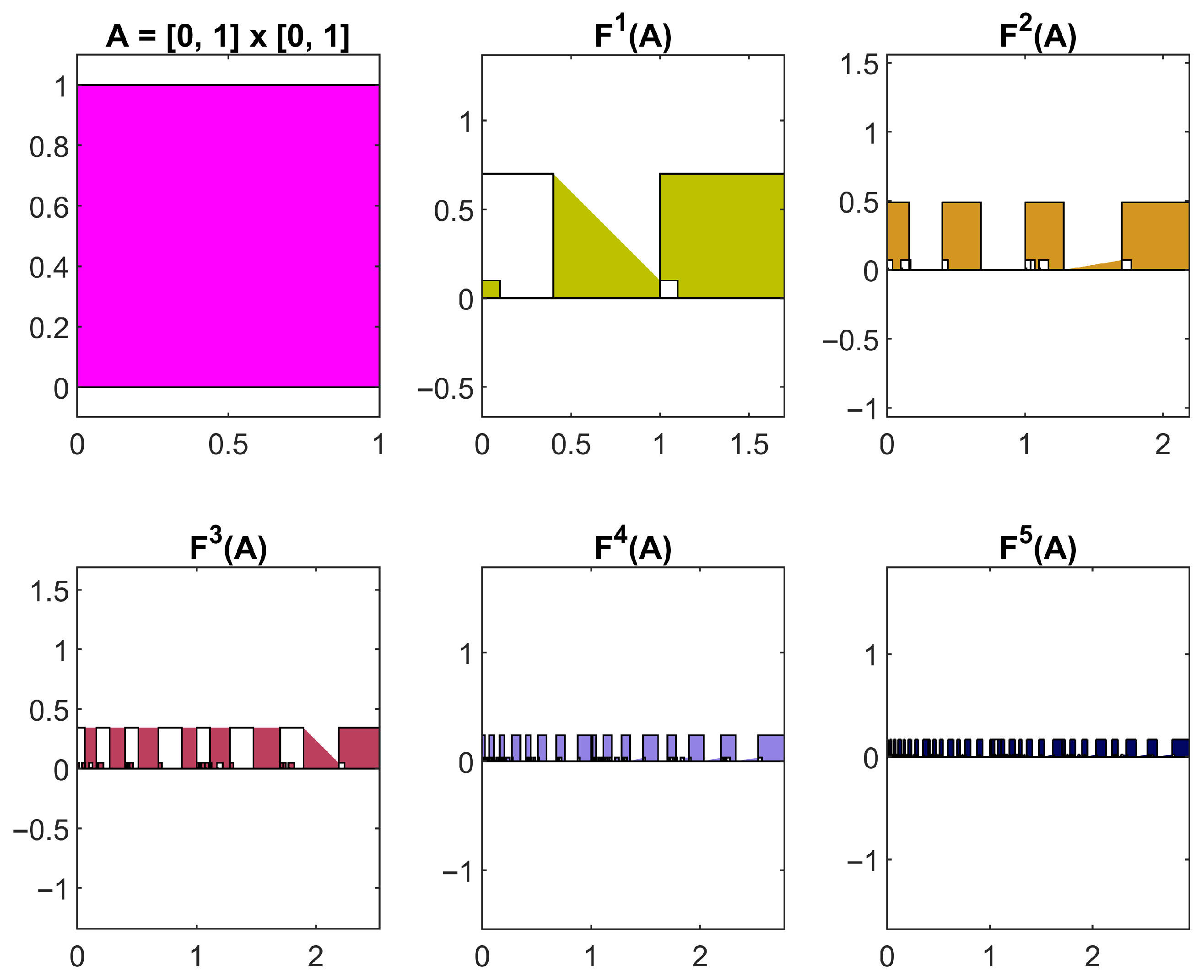
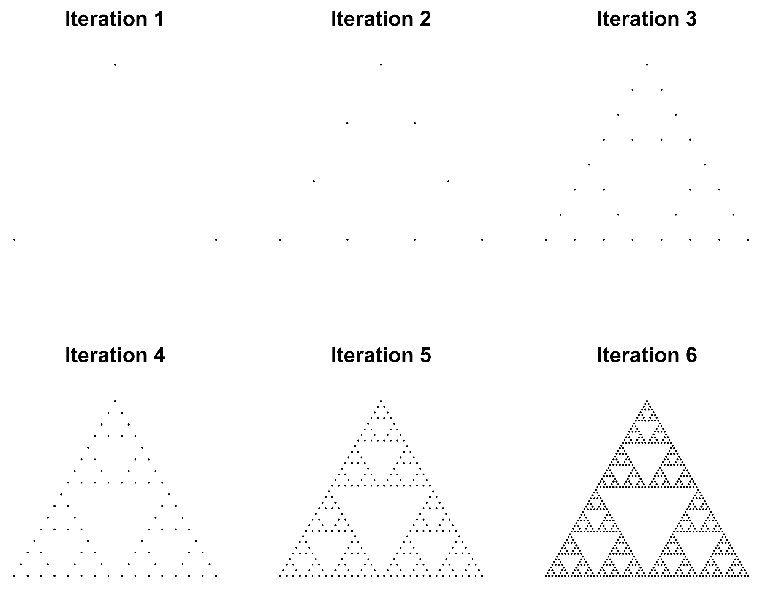
Example 2.

Let $\mathcal{J}=[0,1]\times [0,1]$ be considered under the standard metric and ${\mathcal{T}}_1,{\mathcal{T}}_2:\mathcal{J}\to \mathcal{J}$ be mappings defined by

$${\mathcal{T}}_1(p,q)=\left({\displaystyle \frac{p^2}{2}},{\displaystyle \frac{q^2}{2}}\right);{\mathcal{T}}_2(p,q)=\left({\displaystyle \frac{sinp}{2}},{\displaystyle \frac{sinq}{2}}\right)$$

for each $p,q\in \mathcal{J}$. Further, let $\mathcal{F}\left(\eta \right)=-{\displaystyle \frac{1}{\eta }}(\eta >0),\mathcal{G}\left(\eta \right)=ln\eta ,\phi \left(\eta \right)={\displaystyle \frac{\eta }{2}},{\beta }_1\left(\eta \right)={\beta }_1\left(\eta \right)={\displaystyle \frac{\eta }{1+\eta }}$ and $l_1=l_2={\displaystyle \frac{3}{2}}$. Then, for $p=(p_1,q_1)$ and $q=(p_2,q_2)$ in $\mathcal{J}$ with $p\ne q$, we obtain

$$\begin{array}{ccc}\hfill d({\mathcal{T}}_1\left(p\right),{\mathcal{T}}_1\left(q\right))& =& d\left(\left({\displaystyle \frac{{p_1}^2}{2}},{\displaystyle \frac{{q_1}^2}{2}}\right),\left({\displaystyle \frac{{p_2}^2}{2}},{\displaystyle \frac{{q_2}^2}{2}}\right)\right)\hfill \\ & =& {\displaystyle \frac{1}{2}}\sqrt{{({p_1}^2-{p_2}^2)}^2+{({q_1}^2-{q_2}^2)}^2}\hfill \\ & \le & {\displaystyle \frac{d(p,q)}{2}}-{\displaystyle \frac{1}{ln\left(\frac{{\left(d(p,{\mathcal{T}}_1\left(p\right))\right)}^{\frac{5}{2}}}{1+d(p,{\mathcal{T}}_1\left(p\right))}+\frac{{\left(d(q,{\mathcal{T}}_1\left(q\right))\right)}^{\frac{5}{2}}}{1+d(q,{\mathcal{T}}_1\left(q\right))}\right)}}\hfill \end{array}$$

Similarly,

$$\begin{array}{ccc}\hfill d({\mathcal{T}}_2\left(p\right),{\mathcal{T}}_{2}q)& =& d\left(\left({\displaystyle \frac{sin{p}_1}{2}},{\displaystyle \frac{sin{q}_1}{2}}\right),\left({\displaystyle \frac{sin{p}_2}{2}},{\displaystyle \frac{sin{q}_2}{2}}\right)\right)\hfill \\ & =& {\displaystyle \frac{1}{2}}\sqrt{{({sin{p}_1}^2-{sin{p}_2}^2)}^2+{({sin{q}_1}^2-{sin{q}_2}^2)}^2}\hfill \\ & \le & {\displaystyle \frac{1}{2}}\sqrt{{({p_1}^2-{p_2}^2)}^2+{({q_1}^2-{q_2}^2)}^2}\hfill \\ & \le & {\displaystyle \frac{d(p,q)}{2}}-{\displaystyle \frac{1}{ln\left(\frac{{\left(d(p,{\mathcal{T}}_2\left(p\right))\right)}^{\frac{5}{2}}}{1+d(p,{\mathcal{T}}_2\left(p\right))}+\frac{{\left(d(q,{\mathcal{T}}_2\left(q\right))\right)}^{\frac{5}{2}}}{1+d(q,{\mathcal{T}}_2\left(q\right))}\right)}}.\hfill \end{array}$$

Therefore, in view of (2) the mapping ${\mathcal{T}}_1$ and ${\mathcal{T}}_2$ satisfy the conditions corresponding to the functions $\phi ,\mathcal{G}$, β and any $\mathcal{F}$ defined above.

• Now, consider the IFS $({\mathbb{R}}^2,{\mathcal{T}}_1,{\mathcal{T}}_2)$ with the mappings $\mathcal{W}:K\left(\mathcal{J}\right)\to K\left(\mathcal{J}\right)$ given by

$$\mathcal{W}\left(G\right)={\mathcal{T}}_1\left(G\right)\cup {\mathcal{T}}_2\left(G\right)\mathit{for}\mathit{all}G\in K\left(\mathcal{J}\right).$$

Thus, for each $G,H\in K\left(\mathcal{J}\right)$, we obtain

$$\begin{array}{ccc}\hfill \mathcal{F}\left(\mathfrak{D}\right(\mathcal{T}\left(G\right),\mathcal{T}\left(H\right)\left)\right)& \le & \mathcal{F}\left(\phi \right(\mathfrak{D}(G,H)\left)\right)\hfill \\ & +& \mathcal{G}\left(\beta \left(\mathfrak{D}(G,\mathcal{T}\left(G\right))\right){\left(\mathfrak{D}(G,\mathcal{T}\left(G\right))\right)}^l\right).\hfill \end{array}$$

The IFS fractal resulting from $\mathcal{W}$’s convergence is depicted in Figure 1.

Example 3.

Consider the triangle $\mathcal{A}$ with vertices $\left\{(0,0),(1,0),(0,1)\right\}$ and let $\mathcal{J}=\mathcal{A}\times \mathcal{A}$, endowed with Euclidean metric d. Let ${\mathcal{T}}_1,{\mathcal{T}}_2:\mathcal{J}\to \mathcal{J}$ be mappings defined by

$${\mathcal{T}}_1(p,q)=\left({\displaystyle \frac{1-p}{2}},{\displaystyle \frac{1-q}{2}}\right);{\mathcal{T}}_2(p,q)=\left({sin}^{-1}\left({\displaystyle \frac{p}{4}}\right),{sin}^{-1}\left({\displaystyle \frac{q}{4}}\right)\right)$$

Since $p,q\in [0,1]$, we have $p/4,q/4\in [0,1/4]\subset [-1,1]$; hence, $\mathcal{T}$ is well defined. Further, let $\mathcal{F}\left(\eta \right)=-{\displaystyle \frac{1}{\eta }}(\eta >0),\mathcal{G}\left(\eta \right)=ln\eta ,\phi \left(\eta \right)={\displaystyle \frac{\eta }{2}},{\beta }_1\left(\eta \right)={\beta }_1\left(\eta \right)={\displaystyle \frac{\eta }{1+\eta }}$ and $l_1=l_2={\displaystyle \frac{3}{2}}$. Then, for $p=(p_1,q_1)$ and $q=(p_2,q_2)$ in $\mathcal{J}$ with $p\ne q$, we obtain

$$\begin{array}{ccc}\hfill d({\mathcal{T}}_{1}p,{\mathcal{T}}_{1}q)& =& d\left(\left({\displaystyle \frac{1-p_1}{2}},{\displaystyle \frac{1-q_1}{2}}\right),\left({\displaystyle \frac{1-p_2}{2}},{\displaystyle \frac{1-q_2}{2}}\right)\right)\hfill \\ & =& {\displaystyle \frac{1}{2}}\sqrt{{\left(\left({\displaystyle \frac{1-p_1}{2}}\right)-\left({\displaystyle \frac{1-p_2}{2}}\right)\right)}^2+{\left(\left({\displaystyle \frac{1-q_1}{2}}\right)-\left({\displaystyle \frac{1-q_2}{2}}\right)\right)}^2}\hfill \\ & =& {\displaystyle \frac{1}{2}}\sqrt{{({p_1}^2-{p_2}^2)}^2+{({q_1}^2-{q_2}^2)}^2}\hfill \\ & \le & {\displaystyle \frac{d(p,q)}{2}}-{\displaystyle \frac{1}{ln\left(\frac{{\left(d(p,{\mathcal{T}}_1\left(p\right))\right)}^{\frac{5}{2}}}{1+d(p,{\mathcal{T}}_1\left(p\right))}+\frac{{\left(d(q,{\mathcal{T}}_1\left(q\right))\right)}^{\frac{5}{2}}}{1+d(q,{\mathcal{T}}_1\left(q\right))}\right)}}.\hfill \end{array}$$

Similarly,

$$\begin{array}{ccc}\hfill d({\mathcal{T}}_{2}p,{\mathcal{T}}_{2}q)& =& d\left(\left({sin}^{-1}{\displaystyle \frac{p_1}{4}},{sin}^{-1}{\displaystyle \frac{q_1}{4}}\right),\left({sin}^{-1}{\displaystyle \frac{p_2}{4}},{sin}^{-1}{\displaystyle \frac{q_2}{4}}\right)\right)\hfill \\ & =& \sqrt{{\left({sin}^{-1}{\displaystyle \frac{p_1}{4}}-{sin}^{-1}{\displaystyle \frac{p_2}{4}}\right)}^2+{\left({sin}^{-1}{\displaystyle \frac{q_1}{4}}-{sin}^{-1}{\displaystyle \frac{q_2}{4}}\right)}^2}\hfill \\ & \le & \sqrt{{\left({\displaystyle \frac{p_1}{4}}-{\displaystyle \frac{p_2}{4}}\right)}^2+{\left({\displaystyle \frac{q_1}{4}}-{\displaystyle \frac{q_2}{4}}\right)}^2}\hfill \\ & =& {\displaystyle \frac{1}{4}}\sqrt{{({p_1}^2-{p_2}^2)}^2+{({q_1}^2-{q_2}^2)}^2}\hfill \\ & \le & {\displaystyle \frac{d(p,q)}{2}}-{\displaystyle \frac{1}{ln\left(\frac{{\left(d(p,{\mathcal{T}}_2\left(p\right))\right)}^{\frac{5}{2}}}{1+d(p,{\mathcal{T}}_2\left(p\right))}+\frac{{\left(d(q,{\mathcal{T}}_2\left(q\right))\right)}^{\frac{5}{2}}}{1+d(q,{\mathcal{T}}_2\left(q\right))}\right)}}.\hfill \end{array}$$

Therefore, in view of (2) the mapping ${\mathcal{T}}_1$ and ${\mathcal{T}}_2$ satisfy the conditions corresponding to the functions $\phi ,\mathcal{G}$, β and any $\mathcal{F}$ defined above.

Now, consider the IFS $({\mathbb{R}}^2,{\mathcal{T}}_1,{\mathcal{T}}_2)$ with the mappings $\mathcal{W}:K\left(\mathcal{J}\right)\to K\left(\mathcal{J}\right)$ given by

$$\mathcal{W}\left(G\right)={\mathcal{T}}_1\left(G\right)\cup {\mathcal{T}}_2\left(G\right)\mathit{for}\mathit{all}G\in K\left(\mathcal{J}\right).$$

Thus, for each $G,H\in K\left(\mathcal{J}\right)$, we obtain

$$\begin{array}{ccc}\hfill \mathcal{F}\left(\mathfrak{D}\right(\mathcal{T}\left(G\right),\mathcal{T}\left(H\right)\left)\right)& \le & \mathcal{F}\left(\phi \right(\mathfrak{D}(G,H)\left)\right)\hfill \\ & +& \mathcal{G}\left(\beta \left(\mathfrak{D}(G,\mathcal{T}\left(G\right))\right){\left(\mathfrak{D}(G,\mathcal{T}\left(G\right))\right)}^l\right).\hfill \end{array}$$

The IFS fractal resulting from $\mathcal{W}$’s convergence is depicted in Figure 2.

6. Application to Material Decomposition and Recycling Process

In this section, we develop a theoretical connection of interpolative FG-contractions with fractal geometry; while the framework is mathematical in nature, our aim is to demonstrate its compatibility with physical modeling principles, particularly in systems characterized by stabilization and equilibrium. Rather than presenting explicit kinetic laws or thermodynamic equations, we provide a rigorous operator-theoretic foundation that can be aligned with such physical constraints. The convergence of successive iterations in the Pompeiu–Hausdorff metric ensures stabilization toward a unique fractal, which we interpret as the mathematical analogue of a stable end state in material decomposition or recycling processes. This approach should be understood as a mathematically rigorous framework that is capable of supporting physical models, especially fractional differential systems, rather than as a direct mechanistic description of decomposition dynamics.

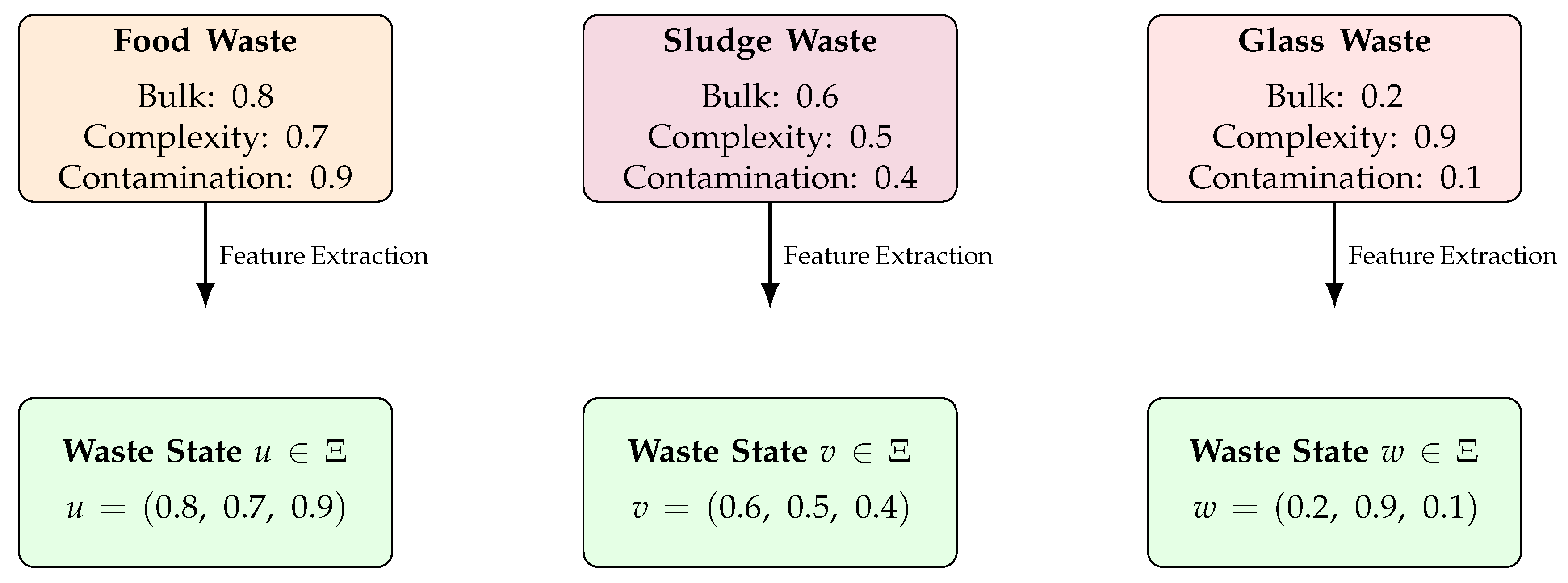
The dissimilarity measure between two waste states $w_1,w_2\in \mathcal{W}$ is represented by the function $d(w_1,w_2)$ (we call it dissimilarity function). It captures quantitative changes in mass, structural complexity, and contamination level. One trash item, such as a metal can or plastic bottle, can be characterized by its matching waste condition, $w_1\in \mathcal{W}$. Different waste states can be compared using a dissimilarity function $d(w_1,w_2)$ to analyze how similar or different materials behave throughout decay processes (see Figure 3).

Multi-Step Abstract Decomposition System

This subsection presents an abstract multi-step dynamical framework motivated by, but not intended to model, real material decomposition or recycling processes. All terminology related to decomposition, stages, or recovery is employed solely as an illustrative analogy to aid intuition. The mathematical results below concern the behavior of nonlinear fractional operators in function spaces and do not rely on, or imply, any physically validated mechanism.

We consider a space of continuous functions $C\left(\right[0,T],\mathbb{R})$ endowed with the metric d defined by

$$d(u,v)=\underset{t\in [0,T]}{sup}|u\left(t\right)-v\left(t\right)|,u,v\in C([0,T],\mathbb{R}).$$

(14)

It is well known that $\left(C\right([0,T],\mathbb{R}),d)$ is a complete metric space.

Let ${\left\{D_n\right\}}_{n=1}^k$ be a finite family of fractional integral operators defined by

$$\left(D_{n}x\right)\left(t\right):=x_0+{\displaystyle \frac{1}{\mathsf{\Gamma }\left({\alpha }_n\right)}}{\int }_0^t{(t-s)}^{{\alpha }_n-1}\left(-{\lambda }_{n}x\left(s\right)+g_n\left(s\right)\right)ds,0<{\alpha }_n<1,$$

where ${\lambda }_n>0$, $g_n\in C([0,T],\mathbb{R})$ are given functions, and $x_0\in \mathbb{R}$ is a prescribed initial value. These operators may be viewed as representing successive transformation stages acting on trajectory functions, without attributing any physical meaning to the individual terms.

Define the associated multi-stage iterated function system (IFS) operator

$$\mathbb{F}:K\left(\mathcal{W}\right)\to K\left(\mathcal{W}\right),\mathbb{F}\left(G\right):={\displaystyle \bigcup _{n=1}^k}{D}_n\left(G\right),$$

where $D_n\left(G\right):=\{D_n\left(x\right):x\in G\}$ and $K\left(\mathcal{W}\right)$ denotes the family of nonempty compact subsets of $\mathcal{W}:=C\left(\right[0,T],\mathbb{R})$.

• Step 1: Compactness. Each operator $D_n$ maps bounded subsets of $\mathcal{W}$ into equicontinuous and uniformly bounded subsets due to the smoothing properties of fractional integral operators. By the Arzelà–Ascoli theorem, $D_n\left(G\right)$ is compact whenever $G\in K\left(\mathcal{W}\right)$. Hence, $\mathbb{F}$ maps $K\left(\mathcal{W}\right)$ into itself.
• Step 2: $\mathcal{F}\mathcal{G}$-contractive property. For any $x,y\in \mathcal{W}$, we have

  $$\parallel D_{n}x-D_n{y\parallel }_{\infty }\le k_n{\parallel x-y\parallel }_{\infty },k_n:={\displaystyle \frac{{\lambda }_n{T}^{{\alpha }_n}}{\mathsf{\Gamma }({\alpha }_n+1)}}<1.$$

  Define $\mathcal{F}\left(u\right)=u$, $\phi \left(u\right)=k_{max}u$ with $k_{max}:=max\{k_1,\dots ,k_k\}$, and let $\mathcal{G}\equiv 0$. Under these choices, each $D_n$ satisfies an interpolative $\mathcal{F}\mathcal{G}$-contractive condition. By Lemma 3.1 (closure of unions of contractions), the operator $\mathbb{F}$ is an $\mathcal{F}\mathcal{G}$-Hutchinson–Barnsley operator on $K\left(\mathcal{W}\right)$.
• Step 3: Application of Theorem 5. Since $\left(K\right(\mathcal{W}),\mathfrak{D})$ is a complete metric space and $\mathbb{F}$ satisfies the $\mathcal{F}\mathcal{G}$-contractive condition, Theorem 5 ensures the following:

  (a)

  There exists a unique nonempty compact set $U\subset \mathcal{W}$, such that

  $$U=\mathbb{F}\left(U\right)={\displaystyle \bigcup _{n=1}^k}{D}_n\left(U\right).$$

  This set represents the invariant attractor of the abstract multi-stage operator system.

  (b)

  For any initial compact set $G_0\in K\left(\mathcal{W}\right)$, the iterative sequence

  $$G_{m+1}=\mathbb{F}\left(G_m\right)$$

  converges to U in the Pompeiu–Hausdorff metric:

  $$\mathfrak{D}(G_m,U)\to 0\mathrm{as}m\to \infty .$$

All conclusions above concern convergence and invariance properties of abstract fractional operators and are independent of any physical interpretation or application.

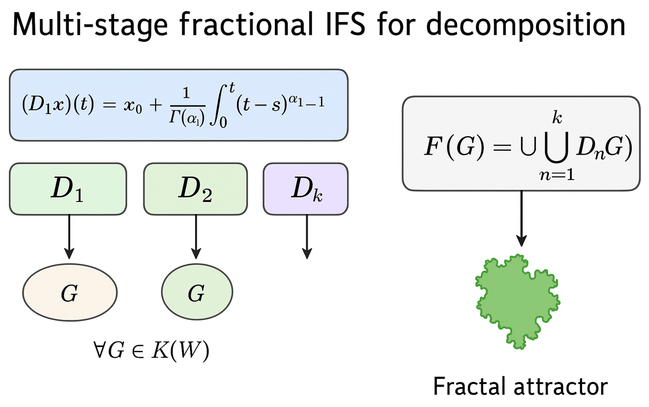
Figure 4 represents the Multi-stage fractional IFS for decomposition.

Note that Example 4 serves as a finite-dimensional analogue or geometric illustration of the convergence behavior described by the abstract operator.

Remark 2.

The purpose of Example 4 is purely illustrative. The terminology of recycling, decomposition, stabilization, or waste states is employed only as a mathematical analogy intended to aid intuition. No physical interpretation, material balance, or experimentally validated degradation mechanism is claimed or implied.

The interpolative $\mathcal{F}\mathcal{G}$-contraction framework and the associated Hutchinson–Barnsley operator are presented as abstract mathematical objects acting on metric spaces. The example serves solely to demonstrate the flexibility of the framework and its ability to generate nontrivial fixed sets and contractive iterative dynamics.

Any connection to physical systems, material behavior, or real-world processes would require additional modeling assumptions, conservation laws, constitutive relations, and experimental calibration, which are deliberately beyond the scope of the present work. The results established here should therefore be viewed as providing a rigorous operator-theoretic structure that could support future physically grounded models, rather than as a validated physical theory.

The following example illustrates how nonlinear decomposition operators generate a contractive Hutchinson–Barnsley system admitting a unique fractal attractor that models long-term redistribution of waste states.

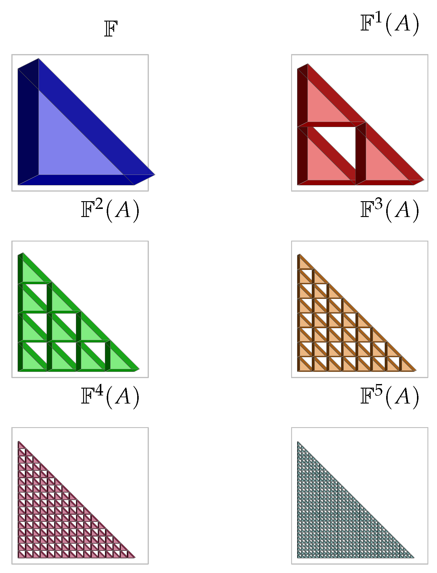
Example 4.

Let $\mathcal{A}$ be a triangular prism in ${\mathbb{R}}^3$, where the triangle provides the basis $\left\{\right(0,0,0),(1,0,0),$$(0,1,0)\}$, and let $\mathcal{W}=\mathcal{A}\subset {\mathbb{R}}^3$ equipped with the metric

$$d\left((w_1,w_2,u),(t_1,t_2,z)\right)=|w_1-t_1|+|w_2-t_2|+|u-z|.$$

Consider two decomposition mappings $D_1,D_2:\mathcal{W}\to \mathcal{W}$ defined by

$$D_1(w_1,w_2,u)=\left(\frac{1-w_1}{2},\frac{1-w_2}{2},\frac{1-u}{2}\right),D_2(w_1,w_2,u)=\left(\frac{arcsin\left(w_1\right)}{4},\frac{arcsin\left(w_2\right)}{4},\frac{arcsin\left(u\right)}{4}\right).$$

Let

$$\mathcal{F}\left(x\right)=ln(1+x),\mathcal{G}\left(x\right)=\frac{1}{2}ln(1+x),\phi \left(x\right)=\frac{x}{2},\beta \left(x\right)=\frac{x}{6}.$$

Take two waste states: food waste $w=(0.8,0.7,0.9)$ and sludge waste $z=(0.6,0.5,0.4)$. Then,

$$d(w,z)=(0.8-0.6)+(0.7-0.5)+(0.9-0.4)=0.9.$$

For $D_1$:

$$D_1\left(w\right)=(0.10,0.15,0.05),D_1\left(z\right)=(0.20,0.25,0.30),$$

and

$$d(D_1\left(w\right),D_1\left(z\right))=0.45=\frac{1}{2}d(w,z).$$

Thus, $D_1$ is a contraction.

Uniform Lipschitz bound for $D_2$. For $D_2\left(x\right)=arcsin\left(x\right)/4$ we have $D_2^{\prime }\left(x\right)=1/\left(4\sqrt{1-x^2}\right)$. Fix $\alpha \in [0,1)$ and restrict all coordinates to $[0,\alpha ]$. Then

$$|D_2^{\prime }\left(x\right)|\le {\displaystyle \frac{1}{4\sqrt{1-{\alpha }^2}}}(x\in [0,\alpha ]),$$

so $D_2$ is Lipschitz on $[0,\alpha ]$ with constant $L\left(\alpha \right)=1/\left(4\sqrt{1-{\alpha }^2}\right)$. Consequently, for any $w,z\in {[0,\alpha ]}^3$,

$$d\left(D_2\left(w\right),D_2\left(z\right)\right)\le L\left(\alpha \right)d(w,z)={\displaystyle \frac{1}{16(1-{\alpha }^2)}}d(w,z).$$

Consequently, for any $w,z\in {[0,\alpha ]}^3$,

$$d\left(D_2\left(w\right),D_2\left(z\right)\right)\le L\left(\alpha \right)d(w,z)={\displaystyle \frac{1}{4\sqrt{1-{\alpha }^2}}}d(w,z).$$

Hence, $D_2$ is a strict contraction on ${[0,\alpha ]}^3$ whenever $\alpha <\sqrt{15}/4\approx 0.968245$.

For clarity,

Table 1. Representative values of the contraction constant.

$\mathit{\alpha }$	$\mathit{L}\left(\mathit{\alpha }\right)=\frac{1}{4\sqrt{1-{\mathit{\alpha }}^2}}$	$\mathit{c}\left(\mathit{\alpha }\right)=\mathit{L}{\left(\mathit{\alpha }\right)}^2$
$0.8$	$0.4167$	$0.1736$
$0.9$	$0.5735$	$0.3289$
$0.95$	$0.8111$	$0.6580$
$1/\sqrt{2}\approx 0.7071$	$0.3536$	$0.1250$

lists several representative values of the contraction constant.

Numerically, for the chosen waste states, we obtain

$$D_2\left(w\right)\approx (0.2318,0.1938,0.2799),D_2\left(z\right)\approx (0.1609,0.1309,0.1029),$$

giving

$$d(D_2\left(w\right),D_2\left(z\right))\approx 0.3108.$$

Thus, in practice, $D_2$ contracts strongly, consistent with the theoretical Lipschitz bound.

In terms of $\mathcal{F}$, one finds

$$\mathcal{F}\left(d(D_2\left(w\right),D_2\left(z\right))\right)=ln\left(1+0.3108\right)\approx 0.2706,$$

while

$$ln\left(1+\frac{d(w,z)}{2}\right)\approx 0.3715,$$

so indeed

$$\mathcal{F}\left(d(D_2\left(w\right),D_2\left(z\right))\right)\le ln\left(1+\frac{d(w,z)}{2}\right).$$

Finally, the associated IFS mapping $\mathbb{F}:K\left(\mathcal{W}\right)\to K\left(\mathcal{W}\right)$ is given by

$$\mathbb{F}\left(G\right)=D_1\left(G\right)\cup D_2\left(G\right),G\in K\left(\mathcal{W}\right),$$

and satisfies the hybrid contractive inequality

$$\mathcal{F}\left(\mathfrak{D}\left(\mathbb{F}\right(G),\mathbb{F}(H\left)\right)\right)\le \mathcal{F}\left(\phi \left(\mathfrak{D}\right(G,H\left)\right)\right)+\mathcal{G}\left(\beta \left(\mathfrak{D}(G,\mathbb{F}\left(G\right))\right){\left(\mathfrak{D}(G,\mathbb{F}\left(G\right))\right)}^l\right).$$

Figure 5 illustrates the geometric structure of the invariant set generated by the Hutchinson–Barnsley operator $\mathbb{F}$ in Example 4. The emergent self-similar geometry reflects the repeated application of nonlinear contractive mappings and serves as a visualization of the fixed-set structure guaranteed by the underlying contraction principles. No physical or material interpretation is implied by this geometry.

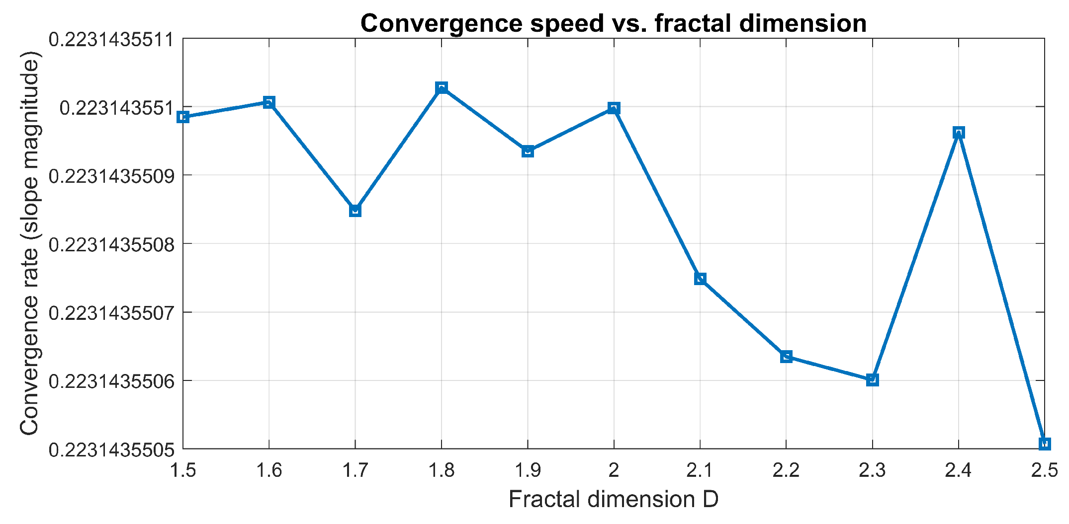
Figure 6 depicts the dependence of the numerical convergence rate of the operator iteration on the prescribed fractal dimension parameter D. The vertical axis represents the magnitude of an empirically estimated exponential decay rate, obtained from the slope of the logarithm of the iteration error norm. As D increases, the observed convergence rate becomes larger in magnitude, indicating faster contraction toward the invariant set. This behavior reflects changes in the geometric complexity of the iterated mappings rather than any notion of physical redistribution or stabilization.

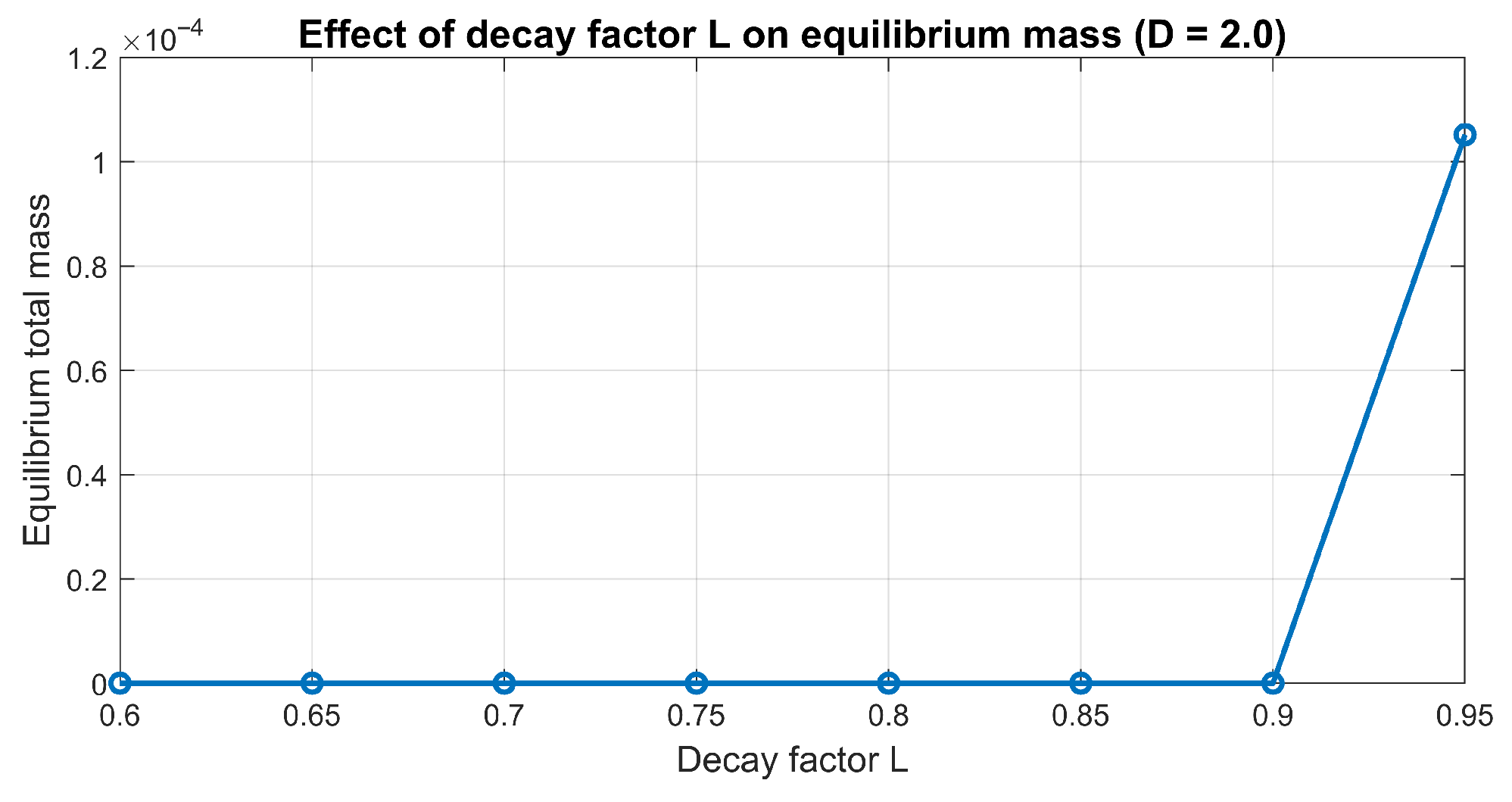
Figure 7 presents the limiting value of a scalar functional of the iterated sets as a function of the local decay parameter L, for fixed fractal dimension $D=2.0$. Smaller values of L are associated with lower limiting functional values, while larger values correspond to higher limiting values. This monotonic dependence illustrates the sensitivity of asymptotic quantities to operator parameters within the abstract iterated function system, without invoking any physical interpretation such as mass conservation or kinetic balance.

7. Conclusions

This paper developed a unified fixed-point framework based on interpolative $\mathcal{F}\mathcal{G}$-contractions and investigated its implications for fractional-order operators and Hutchinson–Barnsley set-valued mappings. The principal theoretical contribution lies in establishing existence and uniqueness results for fixed points and invariant sets under generalized contractive conditions in complete metric spaces.

All illustrative examples and numerical demonstrations were presented at an abstract level and serve only to elucidate the mathematical structure of the framework. No claims regarding physical stabilization, material redistribution, equilibrium states, or experimentally observable behavior are made.

The results provide a rigorous operator-theoretic foundation that could, in future work, be coupled with conservation principles, constitutive modeling, and experimentally informed parameters to yield physically meaningful models. Such extensions fall outside the scope of the present study but represent a natural direction for further research.

References

- Pant, R.; Nashine, H.K. Fractals of FG-Hutchinson Barnsley operator in metric spaces. Filomat 2024, 38, 9711–9725. [Google Scholar] [CrossRef] [Scilit]
- Hutchinson, J.E. Fractals and self similarity. Indiana Univ. Math. J. 1981, 30, 713–747. [Google Scholar] [CrossRef]
- Barnsley, M.F. Fractals Everywhere, 2nd ed.; Academic Press: Cambridge, MA, USA, 1993. [Google Scholar]
- Pant, R. Fixed point theorems for nonlinear contractions with applications to iterated function systems. Appl. Gen. Topol. 2018, 19, 163–172. [Google Scholar] [CrossRef] [Scilit]
- Petrusel, A. Generalized multivalued contractions. Nonlinear Anal. 2001, 47, 649–659. [Google Scholar] [CrossRef] [Scilit]
- Sahu, D.R.; Chakraborty, A.; Dubey, R.P. K-iterated function system. Fractals 2010, 18, 139–144. [Google Scholar] [CrossRef] [Scilit]
- Singh, S.L.; Prasad, B.; Kumar, A. Fractals via iterated functions and multifunctions. Chaos Solitons Fractals 2009, 39, 1224–1231. [Google Scholar] [CrossRef] [Scilit]
- Singh, S.L.; Mishra, S.N.; Jain, S. Orbit of an image under iterated system. Commun. Nonlinear Sci. Numer. 2011, 16, 1469–1482. [Google Scholar] [CrossRef] [Scilit]
- Xu, S.; Cheng, S.; Zhou, Z. Reich’s iterated function systems and well-posedness via fixed point theory. Fixed Point Theory Appl. 2015, 2015, 71. [Google Scholar] [CrossRef] [Scilit]
- Wang, X.Y.; Li, F.P. A class of nonlinear IFS attractors. Nonlinear Anal. 2009, 70, 830–838. [Google Scholar] [CrossRef] [Scilit]
- Dung, N.V.; Petrusel, A. On Iterated Function Systems consisting of Kannan maps, Reich maps, Chatterjea type maps, and related results. J. Fixed Point Theory Appl. 2017, 19, 2271–2285. [Google Scholar] [CrossRef] [Scilit]
- Secelean, N.A. Iterated function systems consisting of F-contractions. Fixed Point Theory Appl. 2013, 2013, 277. [Google Scholar] [CrossRef] [Scilit]
- Nazir, T.; Silvestrov, S.; Abbas, M. Fractals of generalized F-Hutchinson operator. Waves Wavelets Fractals 2016, 2, 29–40. [Google Scholar]
- Secelean, N.A. Generalized F-Iterated function systems on product of metric spaces. J. Fixed Point Theory Appl. 2015, 17, 575–595. [Google Scholar] [CrossRef] [Scilit]
- Banach, S. Sur les opérations dans les ensembles abstraits et leur application aux équations intégrales. Fund. Math. 1922, 3, 133–181. [Google Scholar] [CrossRef] [Scilit]
- Nadler, S.B. Multi-valued contraction mappings. Pacific J. Math. 1969, 30, 475–488. [Google Scholar] [CrossRef] [Scilit]
- Karapinar, E. Revisiting the Kannan type contractions via interpolation. Adv. Theory Nonlinear Anal. Appl. 2018, 2, 85–87. [Google Scholar] [CrossRef] [Scilit]
- Nazam, M.; Lashin, M.M.; Hussain, A.; Sulami, H.H.A. Remarks on the generalized interpolative contractions and some fixed-point theorems with application. Open Math. 2022, 20, 845–862. [Google Scholar] [CrossRef] [Scilit]
- Nazam, M.; Aydi, H.; Hussain, A. Existence theorems for (Ψ,Φ)-orthogonal interpolative contractions and an application to fractional differential equations. Optimization 2023, 72, 1899–1929. [Google Scholar] [CrossRef] [Scilit]
- Parvaneh, V.; Hussain, N.; Kadelburg, Z. Generalized Wardowski type fixed point theorems via α-admissible FG-contractions in b- metric spaces. Acta Math. Sci. 2016, 36, 1445–1456. [Google Scholar] [CrossRef] [Scilit]
- Ahmad, H.; Din, F.U.; Younis, M. A novel Ćirić-Reich-Rus fixed point approach for the existence and uniqueness criterion of a fractional-order Aizawa chaotic system. Chaos Solitons Fractals 2025, 200, 116932. [Google Scholar] [CrossRef] [Scilit]
- Aizawa, Y.; Uezu, T. Global aspects of dissipative dynamical systems. II: Periodic and chaotic responses in the forced Lorenz system. Prog. Theor. Phys. 1982, 68, 1864–1879. [Google Scholar] [CrossRef] [Scilit]
- Toufik, M.; Atangana, A. New numerical approximation of fractional derivative with non-local and non-singular kernel: Application to chaotic models. Eur. Phys. J. Plus 2017, 132, 444. [Google Scholar] [CrossRef] [Scilit]
- Ghanbari, B.; Gómez-Aguilar, J.F. Two efficient numerical schemes for simulating dynamical systems and capturing chaotic behaviors with Mittag–Leffler memory. Eng. Comput. 2022, 38, 2139–2167. [Google Scholar] [CrossRef] [Scilit]
- Jain, S.; El-Khatib, Y. Modelling chaotic dynamical attractor with fractal-fractional differential operators. AIMS Math. 2021, 6, 13689–13725. [Google Scholar] [CrossRef] [Scilit]
- Feng, L.; Liu, Y.; Shi, B.; Liu, J. Toward a physics-guided machine learning approach for predicting chaotic systems dynamics. Front. Big Data 2025, 7, 1506443. [Google Scholar] [CrossRef] [Scilit] [PubMed]
- Lohmiller, W.; Slotine, J.-J.E. On Contraction Analysis for Nonlinear Systems. Automatica 1998, 34, 683–696. [Google Scholar] [CrossRef] [Scilit]