Abundant Non-Traveling Fractal Solutions of Dromion Type for the Extended Hirota–Satsuma–Ito Equation

Abstract

This paper aims to explore non-traveling fractal solutions to an extended Hirota–Satsuma–Ito equation (gHSI) that contains several well-known equations arising in fluid dynamics. Our approach is based on the application of a new variable-separation technique that transfers the governing equation into several solvable forms. Some of these equations can also be solved with standard analytical methods. We employ the modified generalized exponential rational function method (mGERFM), resulting in a varied set of exact analytical solutions. These solutions exhibit a wide range of structural types, such as periodic, rational, hyperbolic, and hybrid configurations. A notable feature of our solutions is that the obtained solutions include several free functions, which provide a systematic way to modify the structure of the waveforms in the solutions. By appropriately selecting these free functions, several categories of dromion-type solutions are introduced. These non-traveling fractal solutions appear to be the first of their kind derived for this equation. The analytical findings are supported by illustrations that demonstrate the complex temporal and spatial dynamics that are characteristic of these solutions. The proposed approach opens a systematic path to non-traveling waves in higher-dimensional systems, where functional flexibility gives rise to self-similar fractal structures, and could be adapted to other equations in physics and engineering.

1. Introduction

Over the past few decades, nonlinear evolution partial differential equations (NEPDEs) have found wide-ranging applications across physics, engineering, and applied mathematics [1,2]. The main applications of these models arise in fluid dynamics, where they govern shallow-water wave propagation and the emergence of coherent structures, such as rogue waves [3,4,5,6].

This paper aims to study the (3 + 1)-dimensional gHSI equation, given by [7,8]

$$\begin{array}{cc}\hfill {\alpha }_1\left[3{\left(u_x{u}_t\right)}_x+u_{xxxt}\right]& +{\alpha }_2\left[3{\left(u_x{u}_y\right)}_x+u_{xxxy}\right]+{\alpha }_3{u}_{yt}\hfill \\ & +{\alpha }_4{u}_{xx}+{\alpha }_5{u}_{xy}+{\alpha }_6{u}_{xt}+{\alpha }_7{u}_{yy}+{\alpha }_8{u}_{zz}=0,\hfill \end{array}$$

(1)

where $u=u(x,y,z,t)$ and ${\alpha }_j$’s ($j=1,2,3,\dots ,8$) are real constants that govern the strength of dispersive and nonlinear effects.

The gHSI Equation (1) constitutes a significant model in the study of nonlinear wave dynamics. Due to this importance, a variety of analytical techniques—including Painlevé analysis [7], symmetry analysis [8], bilinearization, and ansatz-based methods—have been employed to investigate both structural and dynamical properties of the model.

It is worth noting that the variable-coefficient version of the model has also been studied by several authors. The work in [9] studied the variable-coefficient HSI equation via the Hirota bilinear method and the long-wave limit approach. The study also presents breather waves, lump solutions, periodic solutions, and their interactions with solitons. In [10], a variable-coefficient symbolic computation approach was applied to the (2 + 1)-dimensional variable-coefficient HSI equation. Based on their work, various lump-type solutions, including lump, lump–one-soliton, lump–two-solitons, lump–periodic, and lump–soliton–periodic solutions, were obtained. Recently, a (2 + 1)-dimensional generalized variable-coefficient HSI system has been studied in the context of shallow-water wave dynamics in open oceans [11]. In this work, an auto-Bäcklund transformation and three families of solitonic solutions have been derived using a non-characteristic movable singular manifold.

Under appropriate parameter constraints, Equation (1) can be reduced to several important fundamental models in mathematical physics and fluid mechanics. For example,

• If the parameters are constrained such that

  $${\alpha }_4={\alpha }_5={\alpha }_6=0,{\alpha }_7=0,{\alpha }_1={\alpha }_2=1,{\alpha }_3=2,{\alpha }_8=-3,$$

  then the equation results in the well-known (3 + 1)-dimensional Jimbo–Miwa equation [12]

  $$u_{xxxy}+3{\left(u_x{u}_y\right)}_x+2u_{yt}-3u_{zz}=0.$$

  (2)

Equation (2) describes a wide range of physical phenomena occurring in plasma physics and optical systems.

• If the parameters of the model are chosen as

  $${\alpha }_1={\alpha }_4=0,{\alpha }_5={\alpha }_7=0,{\alpha }_2={\alpha }_3=1,{\alpha }_6=-{\alpha }_8=1,$$

  then Equation (1) introduces the model to the (3 + 1)-dimensional Kadomtsev–Petviashvili equation [13].

  $$u_{xxxy}+3{\left(u_x{u}_y\right)}_x+u_{xt}+u_{yt}-u_{zz}=0.$$

  (3)

The obtained equation governs the behavior of (3 + 1)-dimensional solitons in weakly dispersive media and has substantial applications across fluid dynamics and plasma physics.

• A further reduction in the model is achieved by imposing the parameter constraints

  $${\alpha }_1={\alpha }_6=0,{\alpha }_2={\alpha }_3=1,{\alpha }_8=0,{\alpha }_4=\alpha ,{\alpha }_5=\gamma ,{\alpha }_7=\beta .$$

Under these conditions, Equation (1) is simplified to the extended shallow-water wave equation [14]

$$u_{yt}+u_{xxxy}+3{\left(u_x{u}_y\right)}_x+\alpha u_{xx}+\gamma u_{xy}+\beta u_{yy}=0,$$

(4)

which plays a crucial role in describing wave propagation phenomena in oceanography.

• Furthermore, taking ${\alpha }_1=1$ and ${\alpha }_2={\alpha }_8=0$ into account, Equation (1) is reduced to the (2 + 1)-dimensional gHSI equation [15]

  $$3{\left(u_x{u}_t\right)}_x+u_{xxxt}+{\alpha }_3{u}_{yt}+{\alpha }_4{u}_{xx}+{\alpha }_5{u}_{xy}+{\alpha }_6{u}_{xt}+{\alpha }_7{u}_{yy}=0.$$

  (5)

This equation models shallow-water wave phenomena and has been extensively studied for its applications in hydrodynamics and wave theory. The authors of [16] investigated the existence and non-existence of resonant multi-soliton solutions for Equation (5) by employing the linear superposition principle to construct resonant multi-soliton solutions that exhibit inelastic collisions among solitary waves. Moreover, in [17], the Hirota bilinear method and a bilinear Bäcklund transformation technique were used to construct some kink and Breather-wave solutions to the model (5).

• Setting ${\alpha }_1={\alpha }_3={\alpha }_4=1$ and ${\alpha }_2={\alpha }_5={\alpha }_6={\alpha }_7={\alpha }_8=0$ in (1) yields the HSI equation [18]

  $$3{\left(u_x{u}_t\right)}_x+u_{xxxt}+u_{yt}+u_{xx}=0.$$

  (6)
• For ${\alpha }_1=1$, ${\alpha }_4={\alpha }_6=-1$ and ${\alpha }_i=0,$ for $i=2,3,5,7,8$, Equation (1) is transformed into an integrable (1+1)-dimensional HS shallow-water wave system that, under the transformation $\phi =u_x$, is given by [19]

  $$\begin{array}{cc}\hfill {\phi }_t& ={\phi }_{xxt}+3\phi {\phi }_t-3{\phi }_x{v}_t-{\phi }_x,\hfill \\ \hfill v_x& =-\phi ,\hfill \end{array}$$

  (7)

  where $\phi =\phi (x,t)$ and $v=v(x,t)$ are two real-valued functions of space x and time t.
• Finally, Equation (1) under the parameter constraints ${\alpha }_2={\alpha }_6=1,{\alpha }_5={\delta }_1,{\alpha }_7={\delta }_2,$ and ${\alpha }_i=0$ for $i=1,3,4,8,$ is simplified to the generalized Calogero–Bogoyavlenskii–Schiff equation [20,21]

  $$\begin{array}{c}\hfill 3{\left(u_x{u}_y\right)}_x+u_{xxxy}+{\delta }_1{u}_{xy}+u_{xt}+{\delta }_2{u}_{yy}=0.\end{array}$$

  (8)

Several lump solutions to Equation (8) were obtained in [20] by employing a quadratic polynomial ansatz in the Hirota bilinear framework. Also, several breather solutions and their interactions were studied in [21] via homoclinic test functions.

While previous work has greatly improved our knowledge of integrable systems and localized waves, the construction of exact non-traveling wave solutions that depend on arbitrary functions of space and time has not yet been addressed. Such solutions are crucial for describing more realistic physical situations involving inhomogeneities, time-varying boundaries, or external forcing, which are often beyond the scope of classical traveling wave or soliton solutions. To fill this gap, the present work introduces a novel generalized variable-separation transformation technique [22,23,24,25,26] that reduces the original (3 + 1)-dimensional Equation (1) to lower-dimensional forms. By applying the mGERFM to the reduced equations, we derive a rich family of exact non-traveling wave solutions to the main model. One of the main properties of the obtained solutions is the presence of arbitrary functions and free parameters, which enable flexible control over wave profile characteristics. Through appropriate selection of these functional degrees of freedom, the construction of fractal-like dromion structures displaying spatial localization and self-similar patterns is demonstrated.

It is important to distinguish the solutions developed in this work from classical traveling wave solutions, such as solitons, breathers, and lumps, reported in previous works. Traveling wave solutions remain unchanged under translation and describe structures that move through uniform media. In contrast, the non-traveling solutions presented here rely on arbitrary functions of space and time. This flexibility enables them to represent waves interacting with irregular coastlines or turbulent backgrounds. These are scenarios beyond the scope of standard soliton theory.

The remainder of this contribution is organized as follows. In Section 2, a variable-separation idea is used to reduce the model (1) to some reduced solvable forms. Then, a well-known analytical technique, called the mGERFM, is applied in Section 3 to solve one of the reduced forms of the model. Through this implementation, several families of non-traveling wave solutions of the equation are obtained. In Section 4, we visualize the solutions through plots, highlighting the emergence of fractal dromions and the role of arbitrary functions in shaping their self-similar localized profiles. Finally, the paper ends with some concluding remarks.

2. The Main Reduction Strategy

This section presents an extended variable-separation approach designed to generate exact non-traveling wave solutions of Equation (1). The approach relies on the ansatz

$$u(x,y,z,t)=p(y,z,t)·\varphi (\chi ,t)+q(y,z,t),$$

(9)

with the auxiliary variable $\chi$ defined as $\chi =ϵx+\theta (y,z,t)$ within the framework of model (1).

Inserting this ansatz into Equation (1) leads to a simplified form of the equation as

$$\begin{array}{cc}\hfill & {\rho }_1{\displaystyle \frac{{\partial }^4\varphi }{\partial {\chi }^4}}+{\rho }_2{\displaystyle \frac{{\partial }^4\varphi }{\partial {\chi }^3\partial t}}+{\rho }_3{\displaystyle \frac{{\partial }^3\varphi }{\partial {\chi }^3}}+{\rho }_4\left({\displaystyle \frac{\partial \varphi }{\partial \chi }}\right)\left({\displaystyle \frac{{\partial }^2\varphi }{\partial {\chi }^2}}\right)+{\rho }_5\left({\displaystyle \frac{\partial \varphi }{\partial \chi }}\right)\left({\displaystyle \frac{{\partial }^2\varphi }{\partial \chi \partial t}}\right)+{\rho }_6\left({\displaystyle \frac{\partial \varphi }{\partial t}}\right)\left({\displaystyle \frac{{\partial }^2\varphi }{\partial {\chi }^2}}\right)\hfill \\ \hfill & +{\rho }_7{\displaystyle \frac{{\partial }^2\varphi }{\partial {\chi }^2}}+{\rho }_8\varphi {\displaystyle \frac{{\partial }^2\varphi }{\partial {\chi }^2}}+{\rho }_9{\displaystyle \frac{{\partial }^2\varphi }{\partial \chi \partial t}}+{\rho }_{10}{\displaystyle \frac{\partial \varphi }{\partial \chi }}+{\rho }_{11}{\left({\displaystyle \frac{\partial \varphi }{\partial \chi }}\right)}^2+{\rho }_{12}{\displaystyle \frac{\partial \varphi }{\partial t}}+{\rho }_{13}\varphi +{\rho }_{14}=0,\hfill \end{array}$$

(10)

where

$$\begin{array}{cc}\hfill {\rho }_1& =p{ϵ}^3\left({\alpha }_1{\theta }_t+{\alpha }_2{\theta }_y\right),\hfill \\ \hfill {\rho }_2& ={\alpha }_{1}p{ϵ}^3,\hfill \\ \hfill {\rho }_3& ={ϵ}^3\left({\alpha }_1{p}_t+{\alpha }_2{p}_y\right),\hfill \\ \hfill {\rho }_4& =6p^2{ϵ}^2\left({\alpha }_1{\theta }_t+{\alpha }_2{\theta }_y\right),\hfill \\ \hfill {\rho }_5& ={\rho }_6=3{\alpha }_1{p}^2{ϵ}^2,\hfill \\ \hfill {\rho }_7& =p\left[3{ϵ}^2\left({\alpha }_1{q}_t+{\alpha }_2{q}_y\right)+{\alpha }_3{\theta }_y{\theta }_t+{\alpha }_4{ϵ}^2+{\alpha }_5{\theta }_yϵ+{\alpha }_6{\theta }_tϵ+{\alpha }_7{\theta }_y^2+{\alpha }_8{\theta }_z^2\right],\hfill \\ \hfill {\rho }_8& ={\rho }_{11}=3p{ϵ}^2\left({\alpha }_1{p}_t+{\alpha }_2{p}_y\right),\hfill \\ \hfill {\rho }_9& =p\left({\alpha }_3{\theta }_y+{\alpha }_6ϵ\right),\hfill \\ \hfill {\rho }_{10}& ={\alpha }_3\left(p_t{\theta }_y+p{\theta }_{t,y}+p_y{\theta }_t\right)+{\alpha }_5{p}_yϵ+2{\alpha }_7\left(p_y{\theta }_y+\frac{1}{2}p{\theta }_{y,y}\right)+2{\alpha }_8\left(p_z{\theta }_z+\frac{1}{2}p{\theta }_{z,z}\right),\hfill \\ \hfill {\rho }_{12}& ={\alpha }_3{p}_y,\hfill \\ \hfill {\rho }_{13}& ={\alpha }_3{p}_{t,y}+{\alpha }_7{p}_{y,y}+{\alpha }_8{p}_{z,z},\hfill \\ \hfill {\rho }_{14}& ={\alpha }_3{q}_{t,y}+{\alpha }_7{q}_{y,y}+{\alpha }_8{q}_{z,z}.\hfill \end{array}$$

(11)

• In the following theorem, to achieve a convenient simplification, we consider the case where $p(y,z,t)$ is constant; without loss of generality, we assume $p(y,z,t)=1$. From a physical point of view, this choice corresponds to a constant amplitude envelope. It focuses attention on the wave’s phase and spatial structure instead of amplitude variations. This assumption simplifies the analysis while keeping the essential non-traveling wave behavior.

Theorem 1. 

By employing the transformation (9) in the model (1) along with taking $p(y,z,t)=1$, the following cases hold.

(a) 

Let $f_1$ and $f_2$ be arbitrary functions, and define q and θ by

$$\left\{\begin{array}{c}q(y,z,t)=f_1\left(t-{\displaystyle \frac{{\alpha }_1}{{\alpha }_2}}y-{\displaystyle \frac{\sqrt{\Delta }}{{\alpha }_2\sqrt{{\alpha }_8}}}z\right)+f_2\left(t-{\displaystyle \frac{{\alpha }_1}{{\alpha }_2}}y+{\displaystyle \frac{\sqrt{\Delta }}{{\alpha }_2\sqrt{{\alpha }_8}}}z\right)+{\displaystyle \frac{\left(\left(\left(3{\alpha }_1-{\alpha }_4\right){ϵ}^2-{\alpha }_8{c}_1^2\right){\alpha }_3^2+{ϵ}^2{\alpha }_3{\alpha }_6{\alpha }_5-{ϵ}^2{\alpha }_6^2{\alpha }_7\right)}{3{ϵ}^2{\alpha }_2{\alpha }_3^2}}y,\hfill \\ \theta (y,z,t)=-{\displaystyle \frac{ϵ{\alpha }_6}{{\alpha }_3}}y+{\displaystyle \frac{ϵ{\alpha }_6{\alpha }_2}{{\alpha }_1{\alpha }_3}}t+c_{1}z+c_2,\hfill \end{array}\right.$$

(12)

provided that $\Delta :={\alpha }_1{\alpha }_2{\alpha }_3-{\alpha }_1^2{\alpha }_7$ and ${\alpha }_8>0$.

Substituting Equation (12) into Equation (9) reduces the original Equation (1) to the following simplified form:

$$3\left({\displaystyle \frac{{\partial }^2\varphi }{\partial \chi \partial t}}\right)\left({\displaystyle \frac{\partial \varphi }{\partial \chi }}\right)+3\left({\displaystyle \frac{{\partial }^2\varphi }{\partial {\chi }^2}}\right)\left({\displaystyle \frac{\partial \varphi }{\partial t}}\right)+ϵ{\displaystyle \frac{{\partial }^4\varphi }{\partial {\chi }^3\partial t}}+3{\displaystyle \frac{{\partial }^2\varphi }{\partial {\chi }^2}}=0.$$

(13)

(b) 

If the functions q and θ are taken as

$$\left\{\begin{array}{c}\begin{array}{cc}\hfill q(y,z,t)& ={\displaystyle \frac{3{ϵ}^2{\alpha }_1^2}{4({\alpha }_1{\alpha }_7-{\alpha }_2{\alpha }_3)}}{y}^2+{\displaystyle \frac{3{ϵ}^2{\alpha }_1}{4{\alpha }_8}}{z}^2+{\displaystyle \frac{3{\alpha }_2^2{ϵ}^2}{4({\alpha }_1{\alpha }_7-{\alpha }_2{\alpha }_3)}}{t}^2-{\displaystyle \frac{3{ϵ}^2{\alpha }_1{\alpha }_2}{2({\alpha }_1{\alpha }_7-{\alpha }_2{\alpha }_3)}}ty\hfill \\ \hfill & +f_1\left(-{\displaystyle \frac{\sqrt{{\alpha }_8}{\alpha }_{1}y}{2\sqrt{\Delta }}}+{\displaystyle \frac{{\alpha }_2\sqrt{{\alpha }_8}t}{2\sqrt{\Delta }}}-{\displaystyle \frac{z}{2}}\right)+f_2\left(-{\displaystyle \frac{{\alpha }_{1}y}{{\alpha }_2}}+t+{\displaystyle \frac{z\sqrt{\Delta }}{{\alpha }_2\sqrt{{\alpha }_8}}}\right)\hfill \\ \hfill & +{\displaystyle \frac{\left(\begin{array}{c}2{\alpha }_2{\alpha }_3^3(c_1^2{\alpha }_8+{ϵ}^2{\alpha }_4)\\ +{\alpha }_3^2\left((-2{\alpha }_1{\alpha }_4{\alpha }_7-2{\alpha }_2{\alpha }_5{\alpha }_6){ϵ}^2-2{\alpha }_7{\alpha }_8{c}_1^2{\alpha }_1\right)\\ +2{\alpha }_7{ϵ}^2{\alpha }_6({\alpha }_1{\alpha }_5+{\alpha }_2{\alpha }_6){\alpha }_3-2{ϵ}^2{\alpha }_1{\alpha }_6^2{\alpha }_7^2\end{array}\right)}{6{ϵ}^2{\alpha }_2{\alpha }_3^2({\alpha }_1{\alpha }_7-{\alpha }_2{\alpha }_3)}}y\hfill \\ \hfill \theta (y,z,t)& =-{\displaystyle \frac{ϵ{\alpha }_{6}y}{{\alpha }_3}}+{\displaystyle \frac{ϵ{\alpha }_6{\alpha }_{2}t}{{\alpha }_1{\alpha }_3}}+c_{1}z+c_2,\hfill \end{array}\hfill \end{array}\right.$$

(14)

then Equation (9) yields an exact solution to Equation (1), given by

$$\begin{array}{cc}\hfill u_1(x,y,z,t)& =-{\displaystyle \frac{{\left(ϵx-\frac{ϵ{\alpha }_{6}y}{{\alpha }_3}+\frac{ϵ{\alpha }_6{\alpha }_{2}t}{{\alpha }_1{\alpha }_3}+c_{1}z+c_2\right)}^2}{2c_1}}+c_2\left(ϵx-{\displaystyle \frac{ϵ{\alpha }_{6}y}{{\alpha }_3}}+{\displaystyle \frac{ϵ{\alpha }_6{\alpha }_{2}t}{{\alpha }_1{\alpha }_3}}+c_{1}z+c_2\right)+c_{1}t\hfill \\ & +{\displaystyle \frac{3{ϵ}^2{\alpha }_1^2}{4{\alpha }_1{\alpha }_7-4{\alpha }_3{\alpha }_2}}{y}^2+{\displaystyle \frac{3{ϵ}^2{\alpha }_1}{4{\alpha }_8}}{z}^2+{\displaystyle \frac{3{\alpha }_2^2{ϵ}^2}{4{\alpha }_1{\alpha }_7-4{\alpha }_3{\alpha }_2}}{t}^2-{\displaystyle \frac{3{ϵ}^2{\alpha }_2{\alpha }_1}{2\left({\alpha }_1{\alpha }_7-{\alpha }_2{\alpha }_3\right)}}ty\hfill \\ & +f_1\left(-{\displaystyle \frac{\sqrt{{\alpha }_8}{\alpha }_{1}y}{2\sqrt{\Delta }}}+{\displaystyle \frac{{\alpha }_2\sqrt{{\alpha }_8}t}{2\sqrt{\Delta }}}-{\displaystyle \frac{z}{2}}\right)+f_2\left(-{\displaystyle \frac{{\alpha }_{1}y}{{\alpha }_2}}+t+{\displaystyle \frac{z\sqrt{\Delta }}{{\alpha }_2\sqrt{{\alpha }_8}}}\right)\hfill \\ & +{\displaystyle \frac{\left(\begin{array}{c}2{\alpha }_2{\alpha }_3^3(c_1^2{\alpha }_8+{ϵ}^2{\alpha }_4)\\ +{\alpha }_3^2\left((-2{\alpha }_1{\alpha }_4{\alpha }_7-2{\alpha }_2{\alpha }_5{\alpha }_6){ϵ}^2-2{\alpha }_7{\alpha }_8{c}_1^2{\alpha }_1\right)\\ +2{\alpha }_7{ϵ}^2{\alpha }_6({\alpha }_1{\alpha }_5+{\alpha }_2{\alpha }_6){\alpha }_3-2{ϵ}^2{\alpha }_1{\alpha }_6^2{\alpha }_7^2\end{array}\right)}{6{ϵ}^2{\alpha }_2{\alpha }_3^2({\alpha }_1{\alpha }_7-{\alpha }_2{\alpha }_3)}}y+c_3.\hfill \end{array}$$

(15)

(c) 

If the functions q and θ are taken as

$$\left\{\begin{array}{cc}q(y,z,t)\hfill & =\left({\displaystyle \frac{\left({\alpha }_5-6ϵ{\alpha }_2\right){\alpha }_3{\alpha }_6-{\alpha }_3^2{\alpha }_4-{\alpha }_6^2{\alpha }_7}{3{\alpha }_2{\alpha }_3^2}}\right)y+2z{f}_3\left(t\right)+2f_4\left(t\right)\hfill \\ & +f_1\left(t-{\displaystyle \frac{{\alpha }_{1}y}{{\alpha }_2}}+{\displaystyle \frac{z\sqrt{\Delta }}{{\alpha }_2\sqrt{{\alpha }_8}}}\right)+f_2\left(t-{\displaystyle \frac{{\alpha }_{1}y}{{\alpha }_2}}-{\displaystyle \frac{z\sqrt{\Delta }}{{\alpha }_2\sqrt{{\alpha }_8}}}\right)-{\displaystyle \frac{{\alpha }_8}{3{\alpha }_2{ϵ}^2}}{\int }^y{f}_3^2\left(t-{\displaystyle \frac{{\alpha }_1}{{\alpha }_2}}(y-\tau )\right)d\tau ,\hfill \\ \theta (y,z,t)\hfill & =-{\displaystyle \frac{ϵ{\alpha }_6}{{\alpha }_3}}y+z{f}_3\left(t\right)+f_4\left(t\right),\hfill \end{array}\right.$$

(16)

then an exact non-traveling wave solution to Equation (1) is derived as

$$\begin{array}{cc}\hfill u_2(x,y,z,t)& =-2ϵx+\left({\displaystyle \frac{2ϵ{\alpha }_6}{{\alpha }_3}}y+{\displaystyle \frac{\left({\alpha }_5-6ϵ{\alpha }_2\right){\alpha }_3{\alpha }_6-{\alpha }_3^2{\alpha }_4-{\alpha }_6^2{\alpha }_7}{3{\alpha }_2{\alpha }_3^2}}\right)y+\hslash \left(t\right)\hfill \\ & +f_1\left(t-{\displaystyle \frac{{\alpha }_{1}y}{{\alpha }_2}}+{\displaystyle \frac{z\sqrt{\Delta }}{{\alpha }_2\sqrt{{\alpha }_8}}}\right)+f_2\left(t-{\displaystyle \frac{{\alpha }_{1}y}{{\alpha }_2}}-{\displaystyle \frac{z\sqrt{\Delta }}{{\alpha }_2\sqrt{{\alpha }_8}}}\right)-{\displaystyle \frac{{\alpha }_8}{3{\alpha }_2{ϵ}^2}}{\int }^y{f}_3^2\left(t-{\displaystyle \frac{{\alpha }_1}{{\alpha }_2}}(y-\tau )\right)d\tau .\hfill \end{array}$$

(17)

Proof. 

By considering $p(y,z,t)=1$, the coefficients in (11) reduce to

$$\begin{array}{cc}\hfill {\rho }_1& ={\rho }_4/6={ϵ}^3\left({\alpha }_1{\theta }_t+{\alpha }_2{\theta }_y\right),\hfill \\ \hfill {\rho }_2& ={\alpha }_1{ϵ}^3,\hfill \\ \hfill {\rho }_3& ={\rho }_8={\rho }_{11}={\rho }_{12}={\rho }_{13}=0,\hfill \\ \hfill {\rho }_4& =6{ϵ}^2\left({\alpha }_1{\theta }_t+{\alpha }_2{\theta }_y\right),\hfill \\ \hfill {\rho }_5& ={\rho }_6=3{\alpha }_1{ϵ}^2,\hfill \\ \hfill {\rho }_7& =3{ϵ}^2\left({\alpha }_1{q}_t+{\alpha }_2{q}_y\right)+{\alpha }_3{\theta }_y{\theta }_t+{\alpha }_4{ϵ}^2+{\alpha }_5ϵ{\theta }_y+{\alpha }_6ϵ{\theta }_t+{\alpha }_7{\theta }_y^2+{\alpha }_8{\theta }_z^2,\hfill \\ \hfill {\rho }_9& ={\alpha }_3{\theta }_y+{\alpha }_6ϵ,\hfill \\ \hfill {\rho }_{10}& ={\alpha }_3{\theta }_{t,y}+{\alpha }_7{\theta }_{y,y}+{\alpha }_8{\theta }_{z,z},\hfill \\ \hfill {\rho }_{14}& ={\alpha }_3{q}_{t,y}+{\alpha }_7{q}_{y,y}+{\alpha }_8{q}_{z,z}.\hfill \end{array}$$

(18)

(a) 

First, we take the following constraints:

$${\rho }_4={\rho }_9={\rho }_{10}={\rho }_{14}=0,$$

(19)

and

$${\rho }_6={\rho }_7.$$

(20)

Under these assumptions, Equation (10) is then reduced to Equation (12).

(b) 

Taking (11) into account, if we apply the conditions

$${\rho }_1={\rho }_4={\rho }_7={\rho }_9={\rho }_{10}=0,$$

(21)

along with

$${\rho }_6={\rho }_{14},$$

(22)

on Equation (11), then Equation (1) is simplified to

$$\begin{array}{cc}\hfill & ϵ{\displaystyle \frac{{\partial }^4\varphi }{\partial {\chi }^3\partial t}}+3\left({\displaystyle \frac{\partial \varphi }{\partial \chi }}\right)\left({\displaystyle \frac{{\partial }^2\varphi }{\partial \chi \partial t}}\right)+3\left({\displaystyle \frac{{\partial }^2\varphi }{\partial {\chi }^2}}\right)\left({\displaystyle \frac{\partial \varphi }{\partial t}}\right)+3=0.\hfill \end{array}$$

(23)

From Equation (23), we deduce the following exact solution:

$$\begin{array}{cc}\hfill & {\varphi }_1(\chi ,t)=-{\displaystyle \frac{{\chi }^2}{2c_1}}+c_2\chi +c_{1}t+c_3.\hfill \end{array}$$

(24)

It can be deduced that solving system (21) and (22) verifies the results in (14). Conversely, Equation (24) leads directly to the result given in Equation (15).

(c) 

Now, consider

$${\rho }_9={\rho }_{10}={\rho }_{14}=0,$$

(25)

along with

$${\rho }_4={\rho }_7,$$

(26)

in Equation (11), and then we obtain the following equation:

$$\begin{array}{cc}\hfill \left({\alpha }_2{\theta }_y+{\alpha }_1{\theta }_t\right)& \left[6\left({\displaystyle \frac{\partial \varphi (\chi ,t)}{\partial \chi }}\right)\left({\displaystyle \frac{{\partial }^2\varphi (\chi ,t)}{\partial {\chi }^2}}\right)+ϵ{\displaystyle \frac{{\partial }^4\varphi (\chi ,t)}{\partial {\chi }^4}}+6{\displaystyle \frac{{\partial }^2\varphi (\chi ,t)}{\partial {\chi }^2}}\right]\hfill \\ & +{\alpha }_1\left[3\left({\displaystyle \frac{\partial \varphi (\chi ,t)}{\partial \chi }}\right)\left({\displaystyle \frac{{\partial }^2\varphi (\chi ,t)}{\partial \chi \partial t}}\right)+3\left({\displaystyle \frac{\partial \varphi (\chi ,t)}{\partial t}}\right)\left({\displaystyle \frac{{\partial }^2\varphi (\chi ,t)}{\partial {\chi }^2}}\right)+ϵ{\displaystyle \frac{{\partial }^4\varphi (\chi ,t)}{\partial {\chi }^3\partial t}}\right]=0.\hfill \end{array}$$

(27)

Equation (27) suggests the following system of equations for $\varphi (\chi ,t)$ as

$$\left\{\begin{array}{cc}\hfill & 6\left({\displaystyle \frac{\partial \varphi (\chi ,t)}{\partial \chi }}\right)\left({\displaystyle \frac{{\partial }^2\varphi (\chi ,t)}{\partial {\chi }^2}}\right)+ϵ{\displaystyle \frac{{\partial }^4\varphi (\chi ,t)}{\partial {\chi }^4}}+6{\displaystyle \frac{{\partial }^2\varphi (\chi ,t)}{\partial {\chi }^2}}=0,\hfill \\ \hfill & 3\left({\displaystyle \frac{\partial \varphi (\chi ,t)}{\partial \chi }}\right)\left({\displaystyle \frac{{\partial }^2\varphi (\chi ,t)}{\partial \chi \partial t}}\right)+3\left({\displaystyle \frac{\partial \varphi (\chi ,t)}{\partial t}}\right)\left({\displaystyle \frac{{\partial }^2\varphi (\chi ,t)}{\partial {\chi }^2}}\right)+ϵ{\displaystyle \frac{{\partial }^4\varphi (\chi ,t)}{\partial {\chi }^3\partial t}}=0.\hfill \end{array}\right.$$

(28)

Solving Equation (28), we derive the following exact solution:

$$\begin{array}{cc}\hfill & {\varphi }_2\left(\chi ,t\right)=-2\chi +\hslash \left(t\right).\hfill \end{array}$$

(29)

Also, the constraints in (28) lead to the necessary conditions outlined in (16). Moreover, from (9), (16), and (29), the given wave solution in Equation (17) is achieved. □

• While Theorem 1 addressed the special case $p(y,z,t)=1$, Theorem 2 examines the function in its general form.

Theorem 2. 

By employing the transformation

$$u(x,y,z,t)=p(y,z,t)\varphi (\chi ,t)+q(y,z,t),$$

(30)

where $\chi =ϵx+\theta (y,z,t)$ along with ${\alpha }_8>0$ in the nonlinear model (1), the following cases hold.

(a) 

If the functions $p,q$, and θ are taken,

$$\left\{\begin{array}{c}\begin{array}{cc}\hfill p\left(y,z,t\right)& ={\displaystyle \frac{{\alpha }_3{\alpha }_8}{3{ϵ}^2\sqrt{\Delta }\sqrt{{\alpha }_8}z+3{ϵ}^2{\alpha }_2{\alpha }_{8}t-3{ϵ}^2{\alpha }_1{\alpha }_{8}y+c_1{\alpha }_3{\alpha }_8}},\hfill \\ \hfill q\left(y,z,t\right)& =f_1\left(t-{\displaystyle \frac{{\alpha }_{1}y}{{\alpha }_2}}-{\displaystyle \frac{z\sqrt{\Delta }}{{\alpha }_2\sqrt{{\alpha }_8}}}\right)+f_2\left(t-{\displaystyle \frac{{\alpha }_{1}y}{{\alpha }_2}}+{\displaystyle \frac{z\sqrt{\Delta }}{{\alpha }_2\sqrt{{\alpha }_8}}}\right)\hfill \\ & -{\displaystyle \frac{\left(4{\alpha }_7{\alpha }_4{\alpha }_1^2-{\alpha }_5^2{\alpha }_1^2-4{\alpha }_4{\alpha }_3{\alpha }_2{\alpha }_1+2{\alpha }_6{\alpha }_5{\alpha }_2{\alpha }_1-{\alpha }_6^2{\alpha }_2^2\right)y}{12{\alpha }_1{\alpha }_2\left({\alpha }_1{\alpha }_7-{\alpha }_2{\alpha }_3\right)}},\hfill \\ \hfill \theta \left(y,z,t\right)& =-{\displaystyle \frac{ϵ{\alpha }_2\left({ϵ}^2{\alpha }_1-{\alpha }_6\right)t}{{\alpha }_3{\alpha }_1}}+{\displaystyle \frac{ϵ\left({ϵ}^2{\alpha }_1-{\alpha }_6\right)y}{{\alpha }_3}}\hfill \\ & +{\displaystyle \frac{ϵ\left(2{\alpha }_7{ϵ}^2{\alpha }_1^2-2{\alpha }_3{\alpha }_1{ϵ}^2{\alpha }_2+{\alpha }_3{\alpha }_1{\alpha }_5-2{\alpha }_1{\alpha }_6{\alpha }_7+{\alpha }_2{\alpha }_3{\alpha }_6\right)z}{2{\alpha }_3\sqrt{\Delta }\sqrt{{\alpha }_8}}}+c_2,\hfill \end{array}\hfill \end{array}\right.$$

(31)

Equation (1) attains the following exact solution:

$$\begin{array}{cc}\hfill u_3(x,y,z,t)& ={\displaystyle \frac{{\alpha }_3{\alpha }_8\left(-\frac{{\left(ϵx+\theta (y,z,t)\right)}^2}{2}+c_1\left(ϵx+\theta (y,z,t)\right)+\hslash \left(t\right)\right)}{3{ϵ}^2\sqrt{\Delta }\sqrt{{\alpha }_8}z+3{ϵ}^2{\alpha }_2{\alpha }_{8}t-3{ϵ}^2{\alpha }_1{\alpha }_{8}y+c_1{\alpha }_3{\alpha }_8}}+f_1\left(t-{\displaystyle \frac{{\alpha }_{1}y}{{\alpha }_2}}-{\displaystyle \frac{z\sqrt{\Delta }}{{\alpha }_2\sqrt{{\alpha }_8}}}\right)+f_2\left(t-{\displaystyle \frac{{\alpha }_{1}y}{{\alpha }_2}}+{\displaystyle \frac{z\sqrt{\Delta }}{{\alpha }_2\sqrt{{\alpha }_8}}}\right)\hfill \\ & -{\displaystyle \frac{\left(4{\alpha }_7{\alpha }_4{\alpha }_1^2-{\alpha }_5^2{\alpha }_1^2-4{\alpha }_4{\alpha }_3{\alpha }_2{\alpha }_1+2{\alpha }_6{\alpha }_5{\alpha }_2{\alpha }_1-{\alpha }_6^2{\alpha }_2^2\right)y}{12{\alpha }_1{\alpha }_2\left({\alpha }_1{\alpha }_7-{\alpha }_2{\alpha }_3\right)}}.\hfill \end{array}$$

(32)

(b) 

If the functions $p,q$, and θ are taken as

$$\left\{\begin{array}{c}\begin{array}{cc}\hfill p\left(y,z,t\right)& =c_3{\mathrm{e}}^{-{\displaystyle \frac{{ϵ}^3{\alpha }_{2}t}{{\alpha }_3}}+{\displaystyle \frac{{ϵ}^3{\alpha }_{1}y}{{\alpha }_3}}-{\displaystyle \frac{{ϵ}^4\left({\alpha }_3{\alpha }_5{\alpha }_1-2{\alpha }_6{\alpha }_7{\alpha }_1+{\alpha }_3{\alpha }_6{\alpha }_2\right)z}{2c_1{\alpha }_8{\alpha }_3^2}}},\hfill \\ \hfill q\left(y,z,t\right)& =f_1\left(t-{\displaystyle \frac{{\alpha }_{1}y}{{\alpha }_2}}-{\displaystyle \frac{z\sqrt{\Delta }}{{\alpha }_2\sqrt{{\alpha }_8}}}\right)+f_2\left(t-{\displaystyle \frac{{\alpha }_{1}y}{{\alpha }_2}}+{\displaystyle \frac{z\sqrt{\Delta }}{{\alpha }_2\sqrt{{\alpha }_8}}}\right)-{\displaystyle \frac{\left(4{\alpha }_7{\alpha }_4{\alpha }_1^2-{\alpha }_5^2{\alpha }_1^2-4{\alpha }_4{\alpha }_3{\alpha }_2{\alpha }_1+2{\alpha }_6{\alpha }_5{\alpha }_2{\alpha }_1-{\alpha }_6^2{\alpha }_2^2\right)y}{12{\alpha }_1{\alpha }_2\left({\alpha }_1{\alpha }_7-{\alpha }_2{\alpha }_3\right)}},\hfill \\ \hfill \theta \left(y,z,t\right)& ={\displaystyle \frac{ϵ{\alpha }_6{\alpha }_{2}t}{{\alpha }_3{\alpha }_1}}-{\displaystyle \frac{ϵ{\alpha }_{6}y}{{\alpha }_3}}+c_{1}z+c_2,\hfill \end{array}\hfill \end{array}\right.$$

(33)

then Equation (1) attains the following exact solution:

$$\begin{array}{cc}& u_4(x,y,z,t)=c_3\hslash \left(ϵx+{\displaystyle \frac{ϵ{\alpha }_6{\alpha }_{2}t}{{\alpha }_3{\alpha }_1}}-{\displaystyle \frac{ϵ{\alpha }_{6}y}{{\alpha }_3}}+c_{1}z+c_2\right){\mathrm{e}}^{-{\displaystyle \frac{{ϵ}^3{\alpha }_{2}t}{{\alpha }_3}}+{\displaystyle \frac{{ϵ}^3{\alpha }_{1}y}{{\alpha }_3}}-{\displaystyle \frac{{ϵ}^4\left({\alpha }_3{\alpha }_5{\alpha }_1-2{\alpha }_6{\alpha }_7{\alpha }_1+{\alpha }_3{\alpha }_6{\alpha }_2\right)z}{2c_1{\alpha }_8{\alpha }_3^2}}}\hfill \\ & +f_1\left(t-{\displaystyle \frac{{\alpha }_{1}y}{{\alpha }_2}}-{\displaystyle \frac{z\sqrt{\Delta }}{{\alpha }_2\sqrt{{\alpha }_8}}}\right)+f_2\left(t-{\displaystyle \frac{{\alpha }_{1}y}{{\alpha }_2}}+{\displaystyle \frac{z\sqrt{\Delta }}{{\alpha }_2\sqrt{{\alpha }_8}}}\right)-{\displaystyle \frac{\left(4{\alpha }_7{\alpha }_4{\alpha }_1^2-{\alpha }_5^2{\alpha }_1^2-4{\alpha }_4{\alpha }_3{\alpha }_2{\alpha }_1+2{\alpha }_6{\alpha }_5{\alpha }_2{\alpha }_1-{\alpha }_6^2{\alpha }_2^2\right)y}{12{\alpha }_1{\alpha }_2\left({\alpha }_1{\alpha }_7-{\alpha }_2{\alpha }_3\right)}}.\hfill \end{array}$$

(34)

(c) 

If the functions $p,q$, and θ are taken as

$$\left\{\begin{array}{c}\begin{array}{cc}\hfill p\left(y,z,t\right)& =f_1\left(t-{\displaystyle \frac{{\alpha }_{1}y}{{\alpha }_2}}-{\displaystyle \frac{z\sqrt{\Delta }}{{\alpha }_2\sqrt{{\alpha }_8}}}\right),\hfill \\ \hfill q\left(y,z,t\right)& =f_1\left(t-{\displaystyle \frac{{\alpha }_{1}y}{{\alpha }_2}}-{\displaystyle \frac{z\sqrt{\Delta }}{{\alpha }_2\sqrt{{\alpha }_8}}}\right)+f_2\left(t-{\displaystyle \frac{{\alpha }_{1}y}{{\alpha }_2}}+{\displaystyle \frac{z\sqrt{\Delta }}{{\alpha }_2\sqrt{{\alpha }_8}}}\right)\hfill \\ & +{\displaystyle \frac{\left(\begin{array}{c}4{\alpha }_1^3{\alpha }_7{ϵ}^3-4{\alpha }_3{\alpha }_1^2{\alpha }_2{ϵ}^3-4{\alpha }_4{\alpha }_1^2{\alpha }_7{ϵ}^2+{ϵ}^2{\alpha }_1^2{\alpha }_5^2+4{\alpha }_4{\alpha }_3{\alpha }_1{\alpha }_2{ϵ}^2\\ -2{ϵ}^2{\alpha }_1{\alpha }_2{\alpha }_5{\alpha }_6+{ϵ}^2{\alpha }_2^2{\alpha }_6^2-2{\alpha }_3ϵ{\alpha }_1^2{\alpha }_5+4{\alpha }_7ϵ{\alpha }_1^2{\alpha }_6-2{\alpha }_3ϵ{\alpha }_1{\alpha }_2{\alpha }_6+{\alpha }_3^2{\alpha }_1^2\end{array}\right)y}{12{\alpha }_2\left({\alpha }_7{\alpha }_1-{\alpha }_3{\alpha }_2\right){\alpha }_1{ϵ}^2}},\hfill \\ \hfill \theta \left(y,z,t\right)& =-{\displaystyle \frac{ϵ{\alpha }_{6}y}{{\alpha }_3}}+{\displaystyle \frac{ϵ{\alpha }_6{\alpha }_{2}t}{{\alpha }_3{\alpha }_1}}-{\displaystyle \frac{\left(ϵ{\alpha }_1{\alpha }_3{\alpha }_5-2ϵ{\alpha }_1{\alpha }_6{\alpha }_7+ϵ{\alpha }_6{\alpha }_3{\alpha }_2-{\alpha }_1{\alpha }_3^2\right)z}{2\sqrt{\Delta }\sqrt{{\alpha }_8}}}+c_1,\hfill \end{array}\hfill \end{array}\right.$$

(35)

then Equation (1) attains the following exact solution:

$$\begin{array}{cc}\hfill u_5(x,y,z,t)& =c_1\left(-ϵx+{\displaystyle \frac{ϵ{\alpha }_{6}y}{{\alpha }_3}}+{\displaystyle \frac{ϵ{\alpha }_6{\alpha }_2+{\alpha }_3{\alpha }_1}{{\alpha }_3{\alpha }_1}}t-{\displaystyle \frac{\left(ϵ{\alpha }_1{\alpha }_3{\alpha }_5-2ϵ{\alpha }_1{\alpha }_6{\alpha }_7+ϵ{\alpha }_6{\alpha }_3{\alpha }_2-{\alpha }_1{\alpha }_3^2\right)z}{2\sqrt{\Delta }\sqrt{{\alpha }_8}}}+c_2\right)\hfill \\ & \times f_1\left(t-{\displaystyle \frac{{\alpha }_{1}y}{{\alpha }_2}}-{\displaystyle \frac{z\sqrt{\Delta }}{{\alpha }_2\sqrt{{\alpha }_8}}}\right)+f_2\left(t-{\displaystyle \frac{{\alpha }_{1}y}{{\alpha }_2}}+{\displaystyle \frac{z\sqrt{\Delta }}{{\alpha }_2\sqrt{{\alpha }_8}}}\right)\hfill \\ & +{\displaystyle \frac{\left(\begin{array}{c}4{\alpha }_1^3{\alpha }_7{ϵ}^3-4{\alpha }_3{\alpha }_1^2{\alpha }_2{ϵ}^3-4{\alpha }_4{\alpha }_1^2{\alpha }_7{ϵ}^2+{ϵ}^2{\alpha }_1^2{\alpha }_5^2+4{\alpha }_4{\alpha }_3{\alpha }_1{\alpha }_2{ϵ}^2\\ -2{ϵ}^2{\alpha }_1{\alpha }_2{\alpha }_5{\alpha }_6+{ϵ}^2{\alpha }_2^2{\alpha }_6^2-2{\alpha }_3ϵ{\alpha }_1^2{\alpha }_5+4{\alpha }_7ϵ{\alpha }_1^2{\alpha }_6-2{\alpha }_3ϵ{\alpha }_1{\alpha }_2{\alpha }_6+{\alpha }_3^2{\alpha }_1^2\end{array}\right)y}{12{\alpha }_2\left({\alpha }_7{\alpha }_1-{\alpha }_3{\alpha }_2\right){\alpha }_1{ϵ}^2}}.\hfill \end{array}$$

(36)

(d) 

If the functions $p,q$, and θ are taken as

$$\left\{\begin{array}{c}\begin{array}{cc}\hfill p\left(y,z,t\right)& =\left(c_{1}z+c_2\right)\exp \left(t/{\alpha }_1\right),\hfill \\ \hfill q\left(y,z,t\right)& =f_1\left(t-{\displaystyle \frac{{\alpha }_{1}y}{{\alpha }_2}}-{\displaystyle \frac{z\sqrt{\Delta }}{{\alpha }_2\sqrt{{\alpha }_8}}}\right)+f_2\left(t-{\displaystyle \frac{{\alpha }_{1}y}{{\alpha }_2}}+{\displaystyle \frac{z\sqrt{\Delta }}{{\alpha }_2\sqrt{{\alpha }_8}}}\right)-{\displaystyle \frac{\left({\alpha }_4{\alpha }_3^2-{\alpha }_5{\alpha }_3{\alpha }_6+{\alpha }_7{\alpha }_6^2\right)y}{3{\alpha }_2{\alpha }_3^2}},\hfill \\ \hfill \theta \left(y,z,t\right)& =-{\displaystyle \frac{ϵ{\alpha }_{6}y}{{\alpha }_3}}+{\displaystyle \frac{ϵ{\alpha }_2{\alpha }_{6}t}{{\alpha }_1{\alpha }_3}}+c_3,\hfill \end{array}\hfill \end{array}\right.$$

(37)

then Equation (1) attains the following exact solution:

$$\begin{array}{cc}\hfill u_6(x,y,z,t)& =\left(c_{1}z+c_2\right)\left(d_1\left(ϵx-{\displaystyle \frac{ϵ{\alpha }_{6}y}{{\alpha }_3}}+{\displaystyle \frac{ϵ{\alpha }_2{\alpha }_{6}t}{{\alpha }_1{\alpha }_3}}\right)+\hslash \left(t\right)\exp \left(t/{\alpha }_1\right)+d_2\right)\hfill \\ & +f_1\left(t-{\displaystyle \frac{{\alpha }_{1}y}{{\alpha }_2}}-{\displaystyle \frac{z\sqrt{\Delta }}{{\alpha }_2\sqrt{{\alpha }_8}}}\right)+f_2\left(t-{\displaystyle \frac{{\alpha }_{1}y}{{\alpha }_2}}+{\displaystyle \frac{z\sqrt{\Delta }}{{\alpha }_2\sqrt{{\alpha }_8}}}\right)-{\displaystyle \frac{\left({\alpha }_4{\alpha }_3^2-{\alpha }_5{\alpha }_3{\alpha }_6+{\alpha }_7{\alpha }_6^2\right)y}{3{\alpha }_2{\alpha }_3^2}}.\hfill \end{array}$$

(38)

(e) 

If the functions $p,q$, and θ are taken as

$$\left\{\begin{array}{c}\begin{array}{cc}\hfill p\left(y,z,t\right)& =c_1\exp \left(t/{\alpha }_1\right),\hfill \\ \hfill q\left(y,z,t\right)& =f_1\left({\alpha }_{2}t-{\alpha }_{1}y+{\displaystyle \frac{\sqrt{\Delta }z}{\sqrt{{\alpha }_8}}}\right)+f_2\left({\alpha }_{2}t-{\alpha }_{1}y-{\displaystyle \frac{\sqrt{\Delta }z}{\sqrt{{\alpha }_8}}}\right)+c_{2}y,\hfill \\ \hfill \theta \left(y,z,t\right)& =c_4+{\displaystyle \frac{ϵ{\alpha }_6{\alpha }_{2}t}{{\alpha }_1{\alpha }_3}}-{\displaystyle \frac{ϵ{\alpha }_{6}y}{{\alpha }_3}}-{\displaystyle \frac{ϵ\sqrt{{\alpha }_3{\alpha }_5{\alpha }_6-\left(3c_2{\alpha }_2+{\alpha }_4\right){\alpha }_3^2-{\alpha }_7{\alpha }_6^2}z}{{\alpha }_3\sqrt{{\alpha }_8}}},\hfill \end{array}\hfill \end{array}\right.$$

(39)

then Equation (1) attains the following exact solution:

$$\begin{array}{cc}\hfill u_7(x,y,z,t)& =c_{1}sin\left(ϵx+{\displaystyle \frac{ϵ{\alpha }_6{\alpha }_{2}t}{{\alpha }_1{\alpha }_3}}-{\displaystyle \frac{ϵ{\alpha }_{6}y}{{\alpha }_3}}-{\displaystyle \frac{ϵ\sqrt{{\alpha }_3{\alpha }_5{\alpha }_6-\left(3c_2{\alpha }_2+{\alpha }_4\right){\alpha }_3^2-{\alpha }_7{\alpha }_6^2}z}{{\alpha }_3\sqrt{{\alpha }_8}}}+c_4\right)\hfill \\ & +c_{2}cos\left(ϵx+{\displaystyle \frac{ϵ{\alpha }_6{\alpha }_{2}t}{{\alpha }_1{\alpha }_3}}-{\displaystyle \frac{ϵ{\alpha }_{6}y}{{\alpha }_3}}-{\displaystyle \frac{ϵ\sqrt{{\alpha }_3{\alpha }_5{\alpha }_6-\left(3c_2{\alpha }_2+{\alpha }_4\right){\alpha }_3^2-{\alpha }_7{\alpha }_6^2}z}{{\alpha }_3\sqrt{{\alpha }_8}}}+c_4\right)\hfill \\ & +f_1\left({\alpha }_{2}t-{\alpha }_{1}y+{\displaystyle \frac{\sqrt{\Delta }z}{\sqrt{{\alpha }_8}}}\right)+f_2\left({\alpha }_{2}t-{\alpha }_{1}y-{\displaystyle \frac{\sqrt{\Delta }z}{\sqrt{{\alpha }_8}}}\right)+c_{2}y,\hfill \end{array}$$

(40)

provided that $\Delta ,{\alpha }_8,{\alpha }_3{\alpha }_5{\alpha }_6-\left(3c_2{\alpha }_2+{\alpha }_4\right){\alpha }_3^2-{\alpha }_7{\alpha }_6^2$ are all positive values.

Proof. 

By substituting the symbolic ansatz (9) into Equation (1), the equation is reduced to Equation (10), with the corresponding coefficients given in (11). Under this assumption, the following cases occur.

(a) 

In this case, we consider the following assumptions in Equation (11):

$${\rho }_1={\rho }_3={\rho }_4={\rho }_7={\rho }_7={\rho }_{10}={\rho }_{13}={\rho }_{14}=0,$$

(41)

along with

$${\rho }_2={\rho }_9,{\rho }_5={\rho }_{12}.$$

(42)

Taking these constraints, Equation (10) is reformulated to

$$\begin{array}{cc}\hfill & ϵ\left[{\displaystyle \frac{{\partial }^4\varphi }{\partial {\chi }^3\partial t}}+{\displaystyle \frac{{\partial }^2\varphi }{\partial \chi \partial t}}\right]+3p\left[\left({\displaystyle \frac{{\partial }^2\varphi }{\partial \chi \partial t}}\right)\left({\displaystyle \frac{\partial \varphi }{\partial \chi }}\right)+\left({\displaystyle \frac{{\partial }^2\varphi }{\partial {\chi }^2}}\right)\left({\displaystyle \frac{\partial \varphi }{\partial t}}\right)+{\displaystyle \frac{\partial \varphi }{\partial t}}\right]=0.\hfill \end{array}$$

(43)

Equation (43) suggests the following system of equations for $\varphi (\chi ,t)$ as

$$\left\{\begin{array}{cc}\hfill & {\displaystyle \frac{{\partial }^4\varphi (\chi ,t)}{\partial {\chi }^3\partial t}}+{\displaystyle \frac{{\partial }^2\varphi (\chi ,t)}{\partial \chi \partial t}}=0,\hfill \\ \hfill & \left({\displaystyle \frac{{\partial }^2\varphi (\chi ,t)}{\partial \chi \partial t}}\right)\left({\displaystyle \frac{\partial \varphi (\chi ,t)}{\partial \chi }}\right)+\left({\displaystyle \frac{{\partial }^2\varphi (\chi ,t)}{\partial {\chi }^2}}\right)\left({\displaystyle \frac{\partial \varphi (\chi ,t)}{\partial t}}\right)+{\displaystyle \frac{\partial \varphi (\chi ,t)}{\partial t}}=0.\hfill \end{array}\right.$$

(44)

Solving Equation (44), it yields the following exact solution:

$$\begin{array}{cc}\hfill & {\varphi }_3\left(\chi ,t\right)=-{\displaystyle \frac{{\chi }^2}{2}}+c_1\chi +\hslash \left(t\right).\hfill \end{array}$$

(45)

Also, the constraints in (41) and (42) yield the necessary conditions given in (31). So, from (30), (31), and (45), the given wave solution in Equation (32) is obtained.

(b) 

Now, let us consider

$${\rho }_1={\rho }_3={\rho }_4={\rho }_7={\rho }_8={\rho }_9={\rho }_{10}={\rho }_{11}={\rho }_{13}={\rho }_{14}=0,$$

(46)

and

$${\rho }_2={\rho }_{12},$$

(47)

and, in Equation (11), the following reduced equation is constructed:

$$\begin{array}{cc}\hfill & ϵ\left[{\displaystyle \frac{{\partial }^4\varphi }{\partial {\chi }^3\partial t}}+{\displaystyle \frac{\partial \varphi }{\partial t}}\right]+3p\left[\left({\displaystyle \frac{{\partial }^2\varphi }{\partial \chi \partial t}}\right)\left({\displaystyle \frac{\partial \varphi }{\partial \chi }}\right)+\left({\displaystyle \frac{{\partial }^2\varphi }{\partial {\chi }^2}}\right)\left({\displaystyle \frac{\partial \varphi }{\partial t}}\right)\right]=0.\hfill \end{array}$$

(48)

Equation (48) suggests the following system of equations for $\varphi (\chi ,t)$ as

$$\left\{\begin{array}{cc}\hfill & {\displaystyle \frac{{\partial }^4\varphi (\chi ,t)}{\partial {\chi }^3\partial t}}+{\displaystyle \frac{\partial \varphi (\chi ,t)}{\partial t}}=0,\hfill \\ \hfill & \left({\displaystyle \frac{{\partial }^2\varphi (\chi ,t)}{\partial \chi \partial t}}\right)\left({\displaystyle \frac{\partial \varphi (\chi ,t)}{\partial \chi }}\right)+\left({\displaystyle \frac{{\partial }^2\varphi (\chi ,t)}{\partial {\chi }^2}}\right)\left({\displaystyle \frac{\partial \varphi (\chi ,t)}{\partial t}}\right)=0.\hfill \end{array}\right.$$

(49)

Solving Equation (49) yields the following exact solution:

$$\begin{array}{cc}\hfill & {\varphi }_4\left(\chi ,t\right)=\hslash \left(\chi \right).\hfill \end{array}$$

(50)

Furthermore, the conditions in (46) and (47) lead to the given scenario in (33). So, from (30), (33), and (50), the wave solution given in Equation (34) is derived.

(c) 

Now, substituting the constraints

$${\rho }_1={\rho }_3={\rho }_4={\rho }_8={\rho }_9={\rho }_{11}={\rho }_{13}={\rho }_{14}=0,$$

(51)

and

$${\rho }_2={\rho }_7,{\rho }_{10}={\rho }_{12},$$

(52)

into Equation (11) leads to the following equation:

$$\begin{array}{c}\hfill {\alpha }_1{ϵ}^{3}p\left[{\displaystyle \frac{{\partial }^4\varphi }{\partial {\chi }^3\partial t}}+{\displaystyle \frac{{\partial }^2\varphi }{\partial {\chi }^2}}\right]+3{ϵ}^2{\alpha }_1{p}^2\left[\left({\displaystyle \frac{{\partial }^2\varphi }{\partial \chi \partial t}}\right)\left({\displaystyle \frac{\partial \varphi }{\partial \chi }}\right)+\left({\displaystyle \frac{{\partial }^2\varphi }{\partial {\chi }^2}}\right)\left({\displaystyle \frac{\partial \varphi }{\partial t}}\right)\right]+{\alpha }_3{p}_y\left[{\displaystyle \frac{\partial \varphi }{\partial \chi }}+{\displaystyle \frac{\partial \varphi }{\partial t}}\right]=0.\end{array}$$

(53)

Equation (53) suggests the following system of equations for $\varphi (\chi ,x)$ as

$$\left\{\begin{array}{cc}\hfill & {\displaystyle \frac{{\partial }^4\varphi (\chi ,t)}{\partial {\chi }^3\partial t}}+{\displaystyle \frac{{\partial }^2\varphi (\chi ,t)}{\partial {\chi }^2}}=0,\hfill \\ & \left({\displaystyle \frac{{\partial }^2\varphi (\chi ,t)}{\partial \chi \partial t}}\right)\left({\displaystyle \frac{\partial \varphi (\chi ,t)}{\partial \chi }}\right)+\left({\displaystyle \frac{{\partial }^2\varphi (\chi ,t)}{\partial {\chi }^2}}\right)\left({\displaystyle \frac{\partial \varphi (\chi ,t)}{\partial t}}\right)=0,\hfill \\ \hfill & {\displaystyle \frac{\partial \varphi (\chi ,t)}{\partial \chi }}+{\displaystyle \frac{\partial \varphi (\chi ,t)}{\partial t}}=0.\hfill \end{array}\right.$$

(54)

Solving Equation (54), the following exact solution is derived:

$$\begin{array}{c}\hfill {\varphi }_5\left(\chi ,t\right)=\left(t-\chi \right)c_1+c_2.\end{array}$$

(55)

Further, the constraints in (51) and (52) lead to the conditions outlined in (35). Consequently, from (30), (35), and (55), the given non-traveling wave solution in Equation (36) is constructed.

(d) 

In this case, we consider

$${\rho }_1={\rho }_4={\rho }_7={\rho }_9={\rho }_{10}={\rho }_{12}={\rho }_{13}={\rho }_{14}=0,$$

(56)

and

$${\alpha }_1{p}_t+{\alpha }_2{p}_y=p.$$

(57)

Equation (11) is reduced to

$$\begin{array}{c}\hfill ϵ\left[{\displaystyle \frac{{\partial }^3\varphi }{\partial {\chi }^3}}+{\alpha }_1{\displaystyle \frac{{\partial }^4\varphi }{\partial {\chi }^3\partial t}}\right]+3p\left[\left({\displaystyle \frac{{\partial }^2\varphi }{\partial \chi \partial t}}\right)\left({\displaystyle \frac{\partial \varphi }{\partial \chi }}\right)+\left({\displaystyle \frac{{\partial }^2\varphi }{\partial {\chi }^2}}\right)\left({\displaystyle \frac{\partial \varphi }{\partial t}}\right)+\varphi {\displaystyle \frac{{\partial }^2\varphi }{\partial {\chi }^2}}+{\left({\displaystyle \frac{\partial \varphi }{\partial \chi }}\right)}^2\right]=0.\end{array}$$

(58)

Now, from Equation (58), the following system of equations for $\varphi (\chi ,t)$ is constructed:

$$\left\{\begin{array}{cc}\hfill & {\displaystyle \frac{{\partial }^3\varphi (\chi ,t)}{\partial {\chi }^3}}+{\alpha }_1{\displaystyle \frac{{\partial }^4\varphi (\chi ,t)}{\partial {\chi }^3\partial t}}=0,\hfill \\ \hfill & \left({\displaystyle \frac{{\partial }^2\varphi (\chi ,t)}{\partial \chi \partial t}}\right)\left({\displaystyle \frac{\partial \varphi (\chi ,t)}{\partial \chi }}\right)+\left({\displaystyle \frac{{\partial }^2\varphi (\chi ,t)}{\partial {\chi }^2}}\right)\left({\displaystyle \frac{\partial \varphi (\chi ,t)}{\partial t}}\right)+\varphi (\chi ,t){\displaystyle \frac{{\partial }^2\varphi (\chi ,t)}{\partial {\chi }^2}}+{\left({\displaystyle \frac{\partial \varphi (\chi ,t)}{\partial \chi }}\right)}^2=0.\hfill \end{array}\right.$$

(59)

Solving Equation (59), it yields the following exact solution:

$$\begin{array}{c}\hfill {\varphi }_6\left(\chi ,t\right)=d_1\exp \left(-t/{\alpha }_1\right)\chi +\hslash \left(t\right).\end{array}$$

(60)

The provided constraints in Equations (56) and (57) also represent the necessary conditions of Equation (37). Finally, the wave solution in Equation (38) is derived from Equations (30), (37), and (60).

(e) 

Now, by considering

$${\rho }_1={\rho }_4={\rho }_9={\rho }_{10}={\rho }_{12}={\rho }_{14}=0,$$

(61)

along with

$${\alpha }_1{p}_t+{\alpha }_2{p}_y=p,$$

(62)

and

$${\rho }_7={\rho }_{13},$$

(63)

in Equation (11), the following reduced PDE is constructed:

$$\begin{array}{cc}\hfill & {ϵ}^{3}p\left[{\displaystyle \frac{{\partial }^3\varphi }{\partial {\chi }^3}}+{\alpha }_1{\displaystyle \frac{{\partial }^4\varphi }{\partial {\chi }^3\partial t}}\right]+\left({\alpha }_3{p}_{t,y}+{\alpha }_7{p}_{y,y}+{\alpha }_8{p}_{z,z}\right)\left[{\displaystyle \frac{{\partial }^2\varphi (\chi ,t)}{\partial {\chi }^2}}+\varphi (\chi ,t)\right]\hfill \\ \hfill & +3{ϵ}^2{p}^2\left[{\alpha }_1\left({\displaystyle \frac{{\partial }^2\varphi (\chi ,t)}{\partial \chi \partial t}}\right)\left({\displaystyle \frac{\partial \varphi (\chi ,t)}{\partial \chi }}\right)+{\alpha }_1\left({\displaystyle \frac{{\partial }^2\varphi (\chi ,t)}{\partial {\chi }^2}}\right)\left({\displaystyle \frac{\partial \varphi (\chi ,t)}{\partial t}}\right)+\varphi (\chi ,t)\left({\displaystyle \frac{{\partial }^2\varphi (\chi ,t)}{\partial {\chi }^2}}\right)+{\left({\displaystyle \frac{\partial \varphi (\chi ,t)}{\partial \chi }}\right)}^2\right]=0.\hfill \end{array}$$

(64)

From Equation (64), the function $\varphi (\chi ,t)$ satisfies the system constructed below:

$$\left\{\begin{array}{cc}\hfill & {\displaystyle \frac{{\partial }^3\varphi (\chi ,t)}{\partial {\chi }^3}}+{\alpha }_1{\displaystyle \frac{{\partial }^4\varphi (\chi ,t)}{\partial {\chi }^3\partial t}}=0,\hfill \\ \hfill & {\displaystyle \frac{{\partial }^2\varphi (\chi ,t)}{\partial {\chi }^2}}+\varphi (\chi ,t)=0,\hfill \\ & {\alpha }_1\left({\displaystyle \frac{{\partial }^2\varphi (\chi ,t)}{\partial \chi \partial t}}\right)\left({\displaystyle \frac{\partial \varphi (\chi ,t)}{\partial \chi }}\right)+{\alpha }_1\left({\displaystyle \frac{{\partial }^2\varphi (\chi ,t)}{\partial {\chi }^2}}\right)\left({\displaystyle \frac{\partial \varphi (\chi ,t)}{\partial t}}\right)+\varphi (\chi ,t)\left({\displaystyle \frac{{\partial }^2\varphi (\chi ,t)}{\partial {\chi }^2}}\right)+{\left({\displaystyle \frac{\partial \varphi (\chi ,t)}{\partial \chi }}\right)}^2=0.\hfill \end{array}\right.$$

(65)

Solving Equation (65), one gets the following exact solution:

$$\begin{array}{c}\hfill {\varphi }_7\left(\chi ,t\right)=\left(c_{1}sin\left(\chi \right)+c_{2}cos\left(\chi \right)\right)\exp \left(-t/{\alpha }_1\right).\end{array}$$

(66)

Hence, the constraints outlined in (51) and (52) provide the necessary conditions in (35). So, from (30), (35), and (66), the given wave solution in Equation (40) is also retrieved. □

3. Some Non-Traveling Wave Solutions Obtained from Equation (13)

A wide range of analytical methodologies have been developed to construct exact or approximate solutions to nonlinear PDEs. Some notable examples of these methods include the inverse scattering transform, the Hirota bilinear method, the tanh–coth method, the exp-function method, the (G’/G)-expansion method, and various symmetry-based techniques, such as Lie group analysis. Among these techniques, the mGERFM [27] has emerged as a powerful and flexible tool, particularly effective in deriving exact closed-form solutions with rich structural diversity. The implementation proceeds as follows.

• Reduction to equation: Consider the general nonlinear PDE

  $$\mathcal{P}\left(\varphi ,{\varphi }_{\chi },{\varphi }_z,{\varphi }_{tt},\dots \right)=0.$$

  (67)
  Using the traveling wave transformation $\varphi (\chi ,z,t)=u\left(\xi \right)$ with $\xi =\kappa \chi +\omega z+\tau t$, it reduces to

  $$\mathcal{O}\left(u,\kappa u^{\prime },\omega u^{\prime },\tau u^{\prime },\dots \right)=0,$$

  (68)

  where primes denote $d/d\xi$, and $\kappa ,\omega ,\tau$ are parameters to be determined.
• Ansatz: Assume a solution of the form

  $$u\left(\xi \right)={\mathbf{a}}_0+{\displaystyle \sum _{j=1}^{\mathbf{m}}}{\mathbf{a}}_j{\left({\displaystyle \frac{{\Theta }^{\prime }}{\Theta }}\right)}^j+{\displaystyle \sum _{j=1}^{\mathbf{m}}}{\mathbf{b}}_j{\left({\displaystyle \frac{{\Theta }^{\prime }}{\Theta }}\right)}^{-j},$$

  (69)

  where

  $$\Theta \left(\xi \right)={\displaystyle \frac{{\mathbf{r}}_1{e}^{{\mathbf{s}}_1\xi }+{\mathbf{r}}_2{e}^{{\mathbf{s}}_2\xi }}{{\mathbf{r}}_3{e}^{{\mathbf{s}}_3\xi }+{\mathbf{r}}_4{e}^{{\mathbf{s}}_4\xi }}}.$$

  (70)
  Note that the given constants ${\mathbf{r}}_j,{\mathbf{s}}_j$ ($1\le j\le 4$), coefficients ${\mathbf{a}}_0,{\mathbf{a}}_j,{\mathbf{b}}_j$, and the balancing number of the equation $\mathbf{m}$ are chosen so that the ansatz (69) satisfies Equation (68).
• Solution Procedure: Substituting the ansatz into Equation (68) yields a polynomial in exponentials $e^{{\mathbf{s}}_i\xi }$. Setting the coefficients to zero yields a system of polynomial equations in the unknown parameters.
• Final Solution: Solving this system and substituting back into the ansatz yields exact solutions to the original PDE (67).

In what follows, the mGERFM is implemented to solve nonlinear PDE (13), which serves as a reduced form of the original model (1). For this purpose, the following traveling wave variable is considered:

$$\varphi (\chi ,t)=u\left(\xi \right),\xi =\kappa \chi +\tau t.$$

(71)

Under this wave transformation, Equation (13) is transferred to the following ordinary differential equation:

$$\begin{array}{cc}\hfill & ϵ\kappa \tau \left({\displaystyle \frac{d^{4}u\left(\xi \right)}{d{\xi }^4}}\right)+6\tau \left({\displaystyle \frac{d^{2}u\left(\xi \right)}{d{\xi }^2}}\right)\left({\displaystyle \frac{du\left(\xi \right)}{d\xi }}\right)+3{\displaystyle \frac{d^{2}u\left(\xi \right)}{d{\xi }^2}}=0.\hfill \end{array}$$

(72)

Integrating Equation (72) with respect to $\xi$ and neglecting the integration constant yields

$$\begin{array}{cc}\hfill & ϵ\kappa \tau \left({\displaystyle \frac{d^{3}u\left(\xi \right)}{d{\xi }^3}}\right)+3\tau {\left({\displaystyle \frac{du\left(\xi \right)}{d\xi }}\right)}^2+3{\displaystyle \frac{du\left(\xi \right)}{d\xi }}=0.\hfill \end{array}$$

(73)

Also, according to the balancing principle in Equation (73), it is required that $2(\mathbf{m}+1)=\mathbf{m}+3$, which means $\mathbf{m}=1$. Substituting $\mathbf{m}=1$ into Equation (69), the solution of Equation (73) takes the form

$$u\left(\xi \right)={\mathbf{a}}_0+{\mathbf{a}}_1\left({\displaystyle \frac{{\Theta }^{\prime }\left(\xi \right)}{\Theta \left(\xi \right)}}\right)+{\mathbf{b}}_1{\left({\displaystyle \frac{{\Theta }^{\prime }\left(\xi \right)}{\Theta \left(\xi \right)}}\right)}^{-1}.$$

(74)

Under these assumptions, the corresponding solutions to Equation (13) are obtained.

• Set 1: Letting $[{\mathbf{r}}_1,{\mathbf{r}}_2,{\mathbf{r}}_3,{\mathbf{r}}_4]=[1,1,2,0]$ and $[{\mathbf{s}}_1,{\mathbf{s}}_2,{\mathbf{s}}_3,{\mathbf{s}}_4]=[-\mathbf{i},\mathbf{i},0,0]$ in Equation (70) gives

  $$\Theta \left(\xi \right)=cos\left(\xi \right).$$

  (75)

So, the other parameters are obtained as

$$\kappa ={\displaystyle \frac{3}{4ϵ\tau }},{\mathbf{a}}_1={\displaystyle \frac{3}{2\tau }},{\mathbf{b}}_1=0,$$

(76)

while $\tau$ and ${\mathbf{a}}_0$ are free parameters.

Substituting these results into Equations (74), (75), and (71) yields the wave solution for Equation (13) as

$${\varphi }_8(\chi ,t)={\displaystyle \frac{2{\mathbf{a}}_0\tau -3tan\left(\frac{3\chi }{4ϵ\tau }+\tau t\right)}{2\tau }}.$$

(77)

As a consequence, from Equations (9) and (12), a wave solution to Equation (1) is derived as

$$\begin{array}{cc}\hfill u_8(x,y,z,t)& ={\varphi }_8\left(ϵx-{\displaystyle \frac{ϵ{\alpha }_6}{{\alpha }_3}}y+{\displaystyle \frac{ϵ{\alpha }_6{\alpha }_2}{{\alpha }_1{\alpha }_3}}t+c_{1}z+c_2,t\right)+f_1\left(t-{\displaystyle \frac{{\alpha }_1}{{\alpha }_2}}y-{\displaystyle \frac{\sqrt{\Delta }}{{\alpha }_2\sqrt{{\alpha }_8}}}z\right)+f_2\left(t-{\displaystyle \frac{{\alpha }_1}{{\alpha }_2}}y+{\displaystyle \frac{\sqrt{\Delta }}{{\alpha }_2\sqrt{{\alpha }_8}}}z\right)\hfill \\ \hfill & +{\displaystyle \frac{\left(\left(\left(3{\alpha }_1-{\alpha }_4\right){ϵ}^2-{\alpha }_8{c}_1^2\right){\alpha }_3^2+{ϵ}^2{\alpha }_3{\alpha }_6{\alpha }_5-{ϵ}^2{\alpha }_6^2{\alpha }_7\right)}{3{ϵ}^2{\alpha }_2{\alpha }_3^2}}y.\hfill \end{array}$$

(78)

Now, let us consider

$$\kappa ={\displaystyle \frac{3}{16ϵ\tau }},{\mathbf{a}}_1={\displaystyle \frac{3}{8\tau }},{\mathbf{b}}_1=-{\displaystyle \frac{3}{8\tau }},$$

(79)

while $\tau$ and ${\mathbf{a}}_0$ are free parameters.

Inserting these results in Equations (74), (75), and (71) yields the wave solution for Equation (13) as

$${\varphi }_9(\chi ,t)={\displaystyle \frac{8{\mathbf{a}}_0\tau +3cot\left(\frac{3\chi }{16ϵ\tau }+\tau t\right)-3tan\left(\frac{3\chi }{16ϵ\tau }+\tau t\right)}{8\tau }}.$$

(80)

As a result, combining Equations (12) and (71) yields a wave solution to Equation (1) given by

$$\begin{array}{cc}\hfill u_9(x,y,z,t)& ={\varphi }_9\left(ϵx-{\displaystyle \frac{ϵ{\alpha }_6}{{\alpha }_3}}y+{\displaystyle \frac{ϵ{\alpha }_6{\alpha }_2}{{\alpha }_1{\alpha }_3}}t+c_{1}z+c_2,t\right)+f_1\left(t-{\displaystyle \frac{{\alpha }_1}{{\alpha }_2}}y-{\displaystyle \frac{\sqrt{\Delta }}{{\alpha }_2\sqrt{{\alpha }_8}}}z\right)+f_2\left(t-{\displaystyle \frac{{\alpha }_1}{{\alpha }_2}}y+{\displaystyle \frac{\sqrt{\Delta }}{{\alpha }_2\sqrt{{\alpha }_8}}}z\right)\hfill \\ \hfill & +{\displaystyle \frac{\left(\left(\left(3{\alpha }_1-{\alpha }_4\right){ϵ}^2-{\alpha }_8{c}_1^2\right){\alpha }_3^2+{ϵ}^2{\alpha }_3{\alpha }_6{\alpha }_5-{ϵ}^2{\alpha }_6^2{\alpha }_7\right)}{3{ϵ}^2{\alpha }_2{\alpha }_3^2}}y.\hfill \end{array}$$

(81)

• Set 2: Letting $[{\mathbf{r}}_1,{\mathbf{r}}_2,{\mathbf{r}}_3,{\mathbf{r}}_4]=[1,1,1,0]$ and $[{\mathbf{s}}_1,{\mathbf{s}}_2,{\mathbf{s}}_3,{\mathbf{s}}_4]=[1,2,0,0]$ in Equation (70) gives

  $$\Theta \left(\xi \right)={\mathrm{e}}^{\xi }+{\mathrm{e}}^{2\xi }.$$

  (82)

Also, the other parameters are obtained as

$$\kappa =-{\displaystyle \frac{3}{ϵ\tau }},{\mathbf{a}}_1=0,{\mathbf{b}}_1={\displaystyle \frac{12}{\tau }},$$

(83)

while $\tau ,{\mathbf{a}}_0$ are free parameters.

Inserting these results in Equations (74), (82), and (71) yields the wave solution for Equation (13) as

$${\varphi }_{10}(\chi ,t)={\displaystyle \frac{2{\mathbf{a}}_0\tau {\mathrm{e}}^{-\frac{3\chi }{ϵ\tau }+\tau t}+{\mathbf{a}}_0\tau +12{\mathrm{e}}^{-\frac{3\chi }{ϵ\tau }+\tau t}+12}{2\tau {\mathrm{e}}^{-\frac{3\chi }{ϵ\tau }+\tau t}+\tau }}.$$

(84)

As a consequence, from Equations (12) and (71), a wave solution for Equation (1) is derived as

$$\begin{array}{cc}\hfill u_{10}(x,y,z,t)& ={\varphi }_{10}\left(ϵx-{\displaystyle \frac{ϵ{\alpha }_6}{{\alpha }_3}}y+{\displaystyle \frac{ϵ{\alpha }_6{\alpha }_2}{{\alpha }_1{\alpha }_3}}t+c_{1}z+c_2,t\right)+f_1\left(t-{\displaystyle \frac{{\alpha }_1}{{\alpha }_2}}y-{\displaystyle \frac{\sqrt{\Delta }}{{\alpha }_2\sqrt{{\alpha }_8}}}z\right)+f_2\left(t-{\displaystyle \frac{{\alpha }_1}{{\alpha }_2}}y+{\displaystyle \frac{\sqrt{\Delta }}{{\alpha }_2\sqrt{{\alpha }_8}}}z\right)\hfill \\ \hfill & +{\displaystyle \frac{\left(\left(\left(3{\alpha }_1-{\alpha }_4\right){ϵ}^2-{\alpha }_8{c}_1^2\right){\alpha }_3^2+{ϵ}^2{\alpha }_3{\alpha }_6{\alpha }_5-{ϵ}^2{\alpha }_6^2{\alpha }_7\right)}{3{ϵ}^2{\alpha }_2{\alpha }_3^2}}y.\hfill \end{array}$$

(85)

• Set 3: Letting $[{\mathbf{r}}_1,{\mathbf{r}}_2,{\mathbf{r}}_3,{\mathbf{r}}_4]=[\mathbf{i},-\mathbf{i},2,0]$ and $[{\mathbf{s}}_1,{\mathbf{s}}_2,{\mathbf{s}}_3,{\mathbf{s}}_4]=[2-\mathbf{i},2+\mathbf{i},0,0]$ in Equation (70) gives

  $$\Theta \left(\xi \right)={\mathrm{e}}^{2\xi }sin\left(\xi \right).$$

  (86)

Thus, the other parameters are obtained as

$$\kappa ={\displaystyle \frac{3}{4ϵ\tau }},{\mathbf{a}}_1=0,{\mathbf{b}}_1=-{\displaystyle \frac{15}{2\tau }},$$

(87)

while $\tau ,{\mathbf{a}}_0$ are free parameters.

Inserting these results in Equations (74), (86), and (71) yields the wave solution for Equation (13) as

$${\varphi }_{11}(\chi ,t)={\displaystyle \frac{4{\mathbf{a}}_0\tau sin\left(\frac{3\chi }{4ϵ\tau }+\tau t\right)+2{\mathbf{a}}_0\tau cos\left(\frac{3\chi }{4ϵ\tau }+\tau t\right)-15sin\left(\frac{3\chi }{4ϵ\tau }+\tau t\right)}{2\tau \left(cos\left(\frac{3\chi }{4ϵ\tau }+\tau t\right)+2sin\left(\frac{3\chi }{4ϵ\tau }+\tau t\right)\right)}}.$$

(88)

As a consequence, from Equations (12) and (71), a wave solution for Equation (1) is obtained as

$$\begin{array}{cc}\hfill u_{11}(x,y,z,t)& ={\varphi }_{11}\left(ϵx-{\displaystyle \frac{ϵ{\alpha }_6}{{\alpha }_3}}y+{\displaystyle \frac{ϵ{\alpha }_6{\alpha }_2}{{\alpha }_1{\alpha }_3}}t+c_{1}z+c_2,t\right)+f_1\left(t-{\displaystyle \frac{{\alpha }_1}{{\alpha }_2}}y-{\displaystyle \frac{\sqrt{\Delta }}{{\alpha }_2\sqrt{{\alpha }_8}}}z\right)+f_2\left(t-{\displaystyle \frac{{\alpha }_1}{{\alpha }_2}}y+{\displaystyle \frac{\sqrt{\Delta }}{{\alpha }_2\sqrt{{\alpha }_8}}}z\right)\hfill \\ \hfill & +{\displaystyle \frac{\left(\left(\left(3{\alpha }_1-{\alpha }_4\right){ϵ}^2-{\alpha }_8{c}_1^2\right){\alpha }_3^2+{ϵ}^2{\alpha }_3{\alpha }_6{\alpha }_5-{ϵ}^2{\alpha }_6^2{\alpha }_7\right)}{3{ϵ}^2{\alpha }_2{\alpha }_3^2}}y.\hfill \end{array}$$

(89)

• Set 4: Letting $[{\mathbf{r}}_1,{\mathbf{r}}_2,{\mathbf{r}}_3,{\mathbf{r}}_4]=[2,0,1,-1]$ and $[{\mathbf{s}}_1,{\mathbf{s}}_2,{\mathbf{s}}_3,{\mathbf{s}}_4]=[1,0,2,0]$ in Equation (70) gives

  $$\Theta \left(\xi \right)=\mathrm{csch}\left(\xi \right).$$

  (90)

Moreover, the other parameters are obtained as

$$\kappa =-{\displaystyle \frac{3}{4ϵ\tau }},{\mathbf{a}}_1={\displaystyle \frac{3}{2\tau }},{\mathbf{b}}_1=0,$$

(91)

while $\tau$ and ${\mathbf{a}}_0$ are free parameters.

Inserting these results in Equations (74), (90), and (71) yields the wave solution for Equation (13) as

$${\varphi }_{12}(\chi ,t)={\displaystyle \frac{2{\mathbf{a}}_0\tau {\mathrm{e}}^{-\frac{3\chi }{2ϵ\tau }+2\tau t}-2{\mathbf{a}}_0\tau -3{\mathrm{e}}^{-\frac{3\chi }{2ϵ\tau }+2\tau t}-3}{2\tau \left({\mathrm{e}}^{-\frac{3\chi }{2ϵ\tau }+2\tau t}-1\right)}}.$$

(92)

As a consequence, from Equations (12) and (71), a wave solution for Equation (1) is characterized as

$$\begin{array}{cc}\hfill u_{12}(x,y,z,t)& ={\varphi }_{12}\left(ϵx-{\displaystyle \frac{ϵ{\alpha }_6}{{\alpha }_3}}y+{\displaystyle \frac{ϵ{\alpha }_6{\alpha }_2}{{\alpha }_1{\alpha }_3}}t+c_{1}z+c_2,t\right)+f_1\left(t-{\displaystyle \frac{{\alpha }_1}{{\alpha }_2}}y-{\displaystyle \frac{\sqrt{\Delta }}{{\alpha }_2\sqrt{{\alpha }_8}}}z\right)+f_2\left(t-{\displaystyle \frac{{\alpha }_1}{{\alpha }_2}}y+{\displaystyle \frac{\sqrt{\Delta }}{{\alpha }_2\sqrt{{\alpha }_8}}}z\right)\hfill \\ & +{\displaystyle \frac{\left(\left(\left(3{\alpha }_1-{\alpha }_4\right){ϵ}^2-{\alpha }_8{c}_1^2\right){\alpha }_3^2+{ϵ}^2{\alpha }_3{\alpha }_6{\alpha }_5-{ϵ}^2{\alpha }_6^2{\alpha }_7\right)}{3{ϵ}^2{\alpha }_2{\alpha }_3^2}}y.\hfill \end{array}$$

(93)

Remark 1. 

It can be verified that Equation (13) also admits the following wave solution:

$${\varphi }_{13}(\chi ,t)=2ϵc_{2}tanh\left(-{\displaystyle \frac{3t}{4c_2ϵ}}+c_2\chi +c_1\right)+c_3.$$

(94)

As a consequence, from Equations (12) and (71), a non-traveling wave solution to Equation (1) is obtained as

$$\begin{array}{cc}\hfill u_{13}(x,y,z,t)& ={\varphi }_{13}\left(ϵx-{\displaystyle \frac{ϵ{\alpha }_6}{{\alpha }_3}}y+{\displaystyle \frac{ϵ{\alpha }_6{\alpha }_2}{{\alpha }_1{\alpha }_3}}t+c_{1}z+c_2,t\right)+f_1\left(t-{\displaystyle \frac{{\alpha }_1}{{\alpha }_2}}y-{\displaystyle \frac{\sqrt{\Delta }}{{\alpha }_2\sqrt{{\alpha }_8}}}z\right)+f_2\left(t-{\displaystyle \frac{{\alpha }_1}{{\alpha }_2}}y+{\displaystyle \frac{\sqrt{\Delta }}{{\alpha }_2\sqrt{{\alpha }_8}}}z\right)\hfill \\ & +{\displaystyle \frac{\left(\left(\left(3{\alpha }_1-{\alpha }_4\right){ϵ}^2-{\alpha }_8{c}_1^2\right){\alpha }_3^2+{ϵ}^2{\alpha }_3{\alpha }_6{\alpha }_5-{ϵ}^2{\alpha }_6^2{\alpha }_7\right)}{3{ϵ}^2{\alpha }_2{\alpha }_3^2}}y+c_3.\hfill \end{array}$$

(95)

Remark 2. 

All derived solutions in this paper were verified symbolically in Maple to confirm that they satisfy the governing equation.

4. Fractal Dromion Solutions of the gHSI Model (1)

Following our theoretical derivations, this section explores the spatial architecture and localized dynamics of the resulting wave fields. The analytical solutions derived in Section 2 and Section 3 incorporate arbitrary functions $f_1\left(s\right)$ and $f_2\left(s\right)$ that govern the underlying spatial structure of the system. By selecting specific structures in our derived solutions, the fractal-like dromion solutions to the model are characterized in the following subsections.

Also, to quantify the fractal nature of the wave profiles presented in this section, we recall the notion of box-counting (Minkowski) dimension [28].

Definition 1 

(Box-counting dimension). For a bounded set $F\subset {\mathbb{R}}^n$, let $N_{\epsilon }\left(F\right)$ be the minimum number of ε-cubes needed to cover F. The box-counting dimension is

$${dim}_{\mathrm{box}}\left(F\right)=\underset{\epsilon \to 0}{lim}{\displaystyle \frac{log{N}_{\epsilon }\left(F\right)}{log(1/\epsilon )}},$$

when the limit exists. For the graph ${\Gamma }_f=\{(x,f\left(x\right)):x\in I\}$ of a function $f:I\subset \mathbb{R}\to \mathbb{R}$, we have ${dim}_{\mathrm{box}}\left({\Gamma }_f\right)=1$ for smooth functions, while fractal curves satisfy ${dim}_{\mathrm{box}}\left({\Gamma }_f\right)>1$.

Taking this definition into account, the box-counting dimension index will be calculated for selected profiles. The parameter conditions for each solution (as derived in Section 2) are explicitly verified for the values used in the figures.

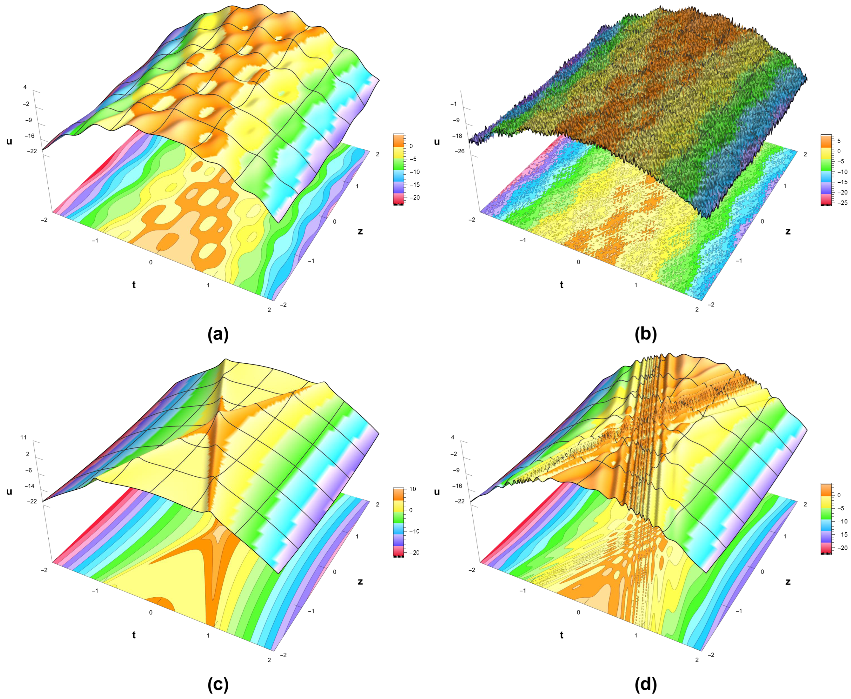
4.1. Fractal Dromion Structures via Solution $u_1$ (Equation (15))

Exponential chirp: Here, let us consider a Gaussian envelope $e^{-0.2s^2}$ times a quadratic-phase carrier $cos(0.5s^2+10s)$ and $sin(0.5s^2+10s)$ as

$$\begin{array}{cc}\hfill \mathbf{\left(}\mathbf{a}\mathbf{\right)}\mathbf{:}& f_1\left(s\right)=e^{-0.2s^2}cos(0.5s^2+10s),f_2\left(s\right)=e^{-0.2s^2}sin(0.5s^2+10s).\hfill \end{array}$$

(96)

Extreme zoom: A Weierstrass-type sum with frequencies ${10}^n$ and amplitudes $0.8^n$. The dromion core is nowhere differentiable and exhibits self-similarity over a wide range of scales. These features are obtained by taking

$$\begin{array}{cc}\hfill \mathbf{\left(}\mathbf{b}\mathbf{\right)}\mathbf{:}& f_1\left(s\right)={\displaystyle \sum _{n=0}^5}0.8^{n}cos\left({10}^{n}s\right),f_2\left(s\right)={\displaystyle \sum _{n=0}^5}0.8^{n}sin\left({10}^{n}s\right).\hfill \end{array}$$

(97)

The Weierstrass-type function satisfies the exact scaling relation $f_1\left(10s\right)={\displaystyle \frac{1}{0.8}}{f}_1\left(s\right)$ for the infinite series, which guarantees self-similarity with scaling factor $\lambda =10$ and amplitude factor $\alpha =log(1/0.8)/log10\approx 0.0969$.

Moreover, for the Weierstrass-type sum in Equation (97),

$$f_1\left(s\right)={\displaystyle \sum _{n=0}^5}0.8^{n}cos\left({10}^{n}s\right),$$

the infinite Weierstrass function $W\left(s\right)={\sum }_{n=0}^{\infty }{a}^{n}cos\left(b^{n}s\right)$ with $a=0.8$, $b=10$ has box-counting dimension ${dim}_{\mathrm{box}}=2+{\displaystyle \frac{loga}{logb}}\approx 1.9031$ (see Definition 1). While our finite truncation yields an approximately fractal structure, the box-counting dimension computed numerically from the profile in Figure 1b is approximately $1.89$, consistent with the expected theoretical value.

Cantor Gaussian: A Cantor-set construction using Gaussians placed at positions $1/3^n$ with widths $3^{-n}$. The dromion core exhibits exact three-fold self-similarity across five generations. The structure is given by

$$\begin{array}{cc}\hfill \mathbf{\left(}\mathbf{c}\mathbf{\right)}\mathbf{:}& f_1\left(s\right)={\displaystyle \sum _{n=0}^5}{e}^{-3^n{(s-1/3^n)}^2},f_2\left(s\right)={\displaystyle \sum _{n=0}^5}{e}^{-3^n{(s-1/3^n)}^2}.\hfill \end{array}$$

(98)

The positions $s_n=1/3^n$ and widths ${\sigma }_n=3^{-n}$ follow a geometric progression with scaling factor $\lambda =3$. Each generation n contains $2^n$ Gaussians, reproducing the classical Cantor-set construction. The self-similarity relation $f\left(s\right)\approx {\displaystyle \frac{1}{2}}f\left(3s\right)$ holds approximately over the support.

Log-periodic dromion: A Gaussian envelope multiplied by $cos(5log(s^2+0.001))$ and $sin(5log(s^2+0.001))$. The dromion core exhibits nested and log-periodic oscillations whose spacing follows a geometric progression. The formula is

$$\begin{array}{cc}\hfill \mathbf{\left(}\mathbf{d}\mathbf{\right)}\mathbf{:}& f_1\left(s\right)=e^{-s^2}cos\left(5log(s^2+0.001)\right),f_2\left(s\right)=e^{-s^2}sin\left(5log(s^2+0.001)\right).\hfill \end{array}$$

(99)

Using Equations (96)–(99) together with the parameter set

$$\begin{array}{c}\hfill {\alpha }_1=1.7,{\alpha }_2=1,{\alpha }_3=2.5,{\alpha }_4=0.1,{\alpha }_5=0.2,{\alpha }_6=0.5,{\alpha }_7=0.7,{\alpha }_8=0.5,\mathrm{and}{c}_1=c_2=1,c_3=0,\end{array}$$

(100)

dromion solutions obtained from (15) are displayed in Figure 1. It is worth noting that the parameter set in (100) is chosen to satisfy all positivity constraints stated after Equation (15) in Section 2; the same consideration is applied in the same cases throughout the paper.

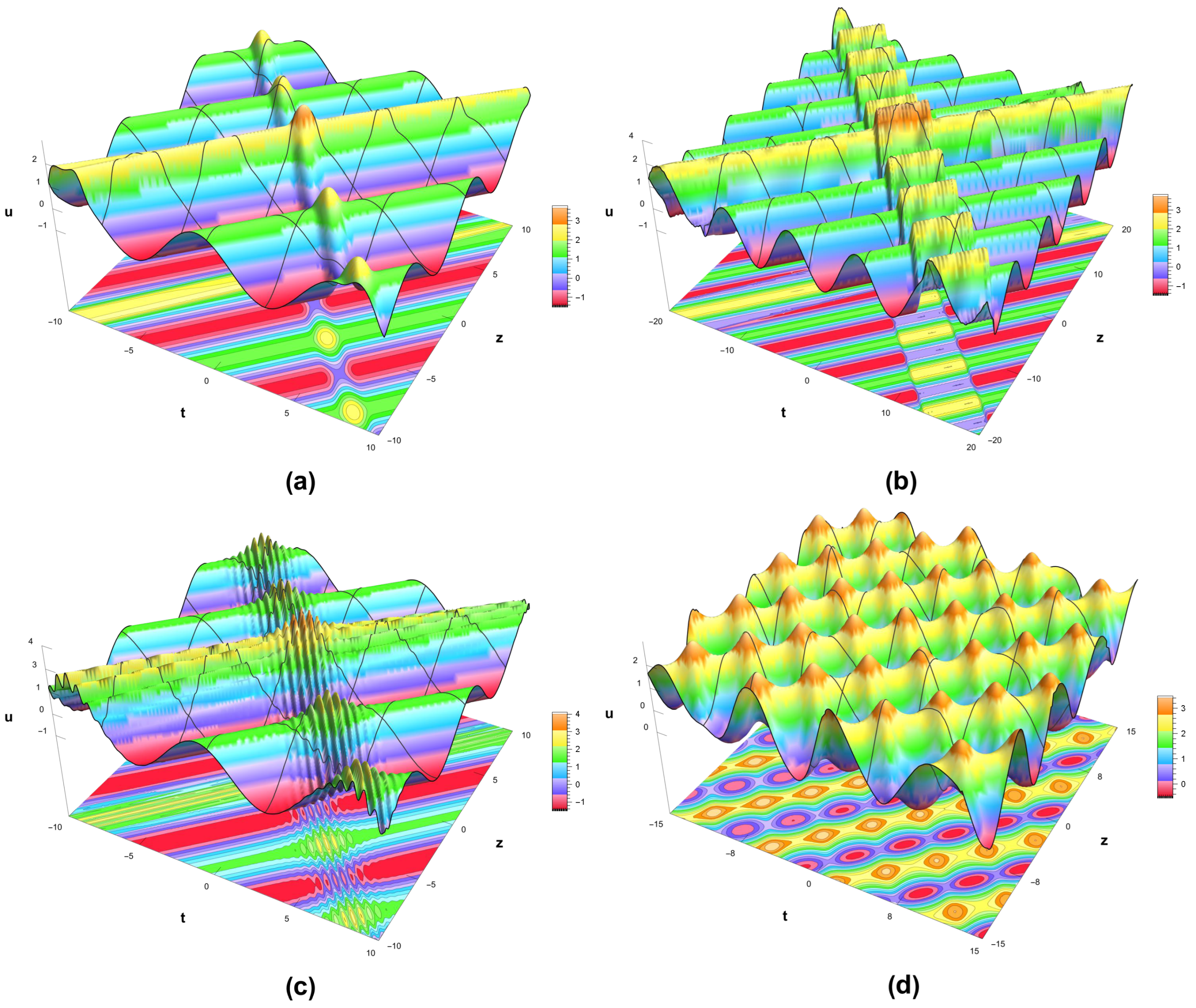
4.2. Fractal Dromion Structures via Solution $u_7$ (Equation (40))

Anharmonic potential: A quartic anharmonic term modifies the Gaussian envelope. The first function $e^{-s^4-s^2}$ produces a flattened peak, whereas $e^{-s^4+s^2}$ creates a double-well structure. This structure is given by

$$\begin{array}{cc}\hfill \mathbf{\left(}\mathbf{a}\mathbf{\right)}\mathbf{:}& f_1\left(s\right)=e^{-s^4-s^2},f_2\left(s\right)=e^{s^2-s^4}.\hfill \end{array}$$

(101)

Gaussian fractal: A superposition of narrow Gaussians centered at half-integer positions from $-4$ to 4 in steps of $0.5$. The resulting dromion core consists of a dense comb of nearly non-overlapping peaks. So, let

$$\begin{array}{cc}\hfill \mathbf{\left(}\mathbf{b}\mathbf{\right)}\mathbf{:}& f_1\left(s\right)={\displaystyle \sum _{n=-4}^4}{e}^{-{(s+n)}^2/0.1},f_2\left(s\right)={\displaystyle \sum _{m=-4}^4}{e}^{-{(s+m)}^2/0.1}.\hfill \end{array}$$

(102)

Complex mod-sech: The sech envelope is modulated by a slow oscillation $1+0.5cos\left(10s\right)$ (and similarly with sin). This creates a train of sub-peaks within the localized core. Now, we take

$$\begin{array}{cc}\hfill \mathbf{\left(}\mathbf{c}\mathbf{\right)}\mathbf{:}& f_1\left(s\right)=sech\left(s\right)\left(1+0.5cos\left(10s\right)\right),f_2\left(s\right)=sech\left(s\right)\left(1+0.5sin\left(10s\right)\right).\hfill \end{array}$$

(103)

A remarkable property is that the modulation depth of $0.5$ is less than unity, so the envelope remains positive, yielding a fine internal structure that resembles a soliton with an imprinted periodic pattern.

Double-periodic DN: Jacobi elliptic functions $dn(s,0.95)$ and $dn(s,0.5)$. The two components have different moduli, producing a quasiperiodic dromion core with two incommensurate periods. The structure is given by

$$\begin{array}{cc}\hfill \mathbf{\left(}\mathbf{d}\mathbf{\right)}\mathbf{:}& f_1\left(s\right)=dn(s,0.95),f_2\left(s\right)=dn(s,0.5).\hfill \end{array}$$

(104)

A notable feature is that $dn(s,0.95)$ is nearly constant (close to 1) with very narrow dips, while $dn(s,0.5)$ varies more smoothly, leading to a complex quasiperiodic pattern.

Using Equations (101), (102), (103) and (104) together with the parameter set

$$\begin{array}{c}\hfill {\alpha }_1=0.6,{\alpha }_2=1,{\alpha }_3=1.6,{\alpha }_4=1,{\alpha }_5=10,{\alpha }_6=0.75,{\alpha }_7=0.25,{\alpha }_8=1,\mathrm{and}{c}_1=c_2=1,c_4=0,\end{array}$$

(105)

dromion solutions obtained from (40) are shown in Figure 2.

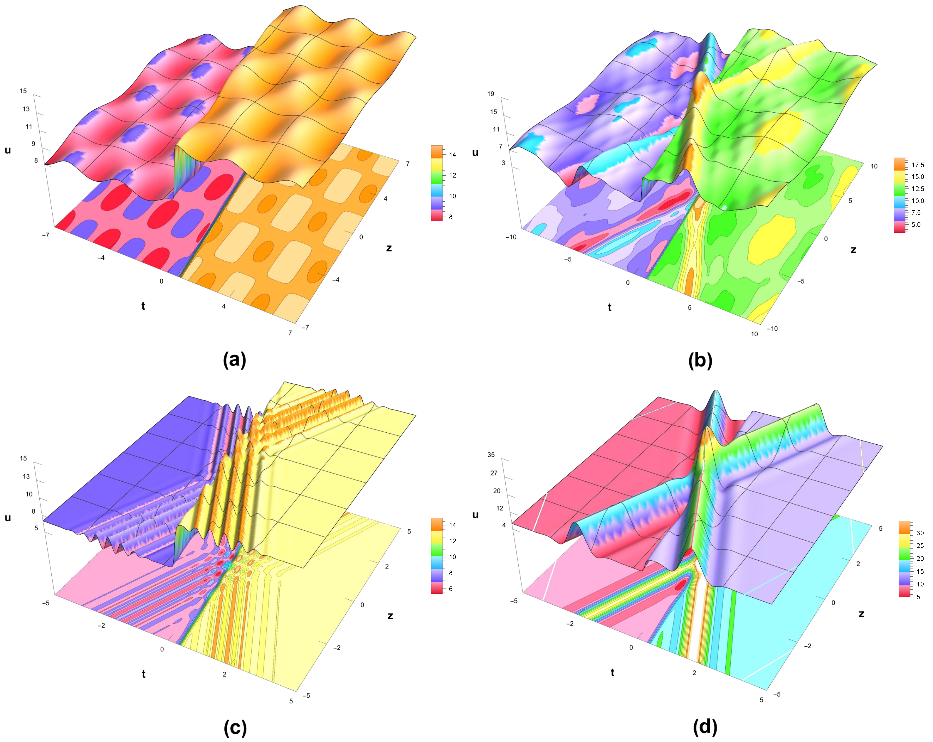
4.3. Fractal Dromion Structures via Solution $u_{10}$ (Equation (85))

Tanh-pulse train: A sum of box-like pulses constructed from tanh differences: $tanh(s+3n)-tanh(s+3n-1)$. The dromion core is a periodic train of nearly rectangular pulses, each of unit width and spacing 3. The formula is

$$\begin{array}{cc}\hfill \mathbf{\left(}\mathbf{a}\mathbf{\right)}\mathbf{:}& f_1\left(s\right)=\underset{n=-3}{\sum ^3}(tanh(-3n-s+1)+tanh(3n+s)),f_2\left(s\right)=\underset{m=-3}{\sum ^3}(tanh(-3m-s+1)+tanh(3m+s)).\hfill \end{array}$$

(106)

Each tanh difference approximates a Heaviside step, so the sum produces a piecewise-constant train with sharp but smooth edges, a localized “top-hat” comb.

Sqrt harmonic sum: A sum of $sin\left(\sqrt{n}s\right)/n$ and $cos\left(\sqrt{n}s\right)/n$ up to $n=15$. The frequencies grow as $\sqrt{n}$, producing a slowly increasing chirp, a “square-root” dromion. Let us take

$$\begin{array}{cc}\hfill \mathbf{\left(}\mathbf{b}\mathbf{\right)}\mathbf{:}& f_1\left(s\right)=\underset{n=1}{\sum ^{15}}{\displaystyle \frac{sin\left(\sqrt{n}s\right)}{n}},f_2\left(s\right)=\underset{n=1}{\sum ^{15}}{\displaystyle \frac{cos\left(\sqrt{n}s\right)}{n}}.\hfill \end{array}$$

(107)

The chirp rate $d\omega /dn=1/\left(2\sqrt{n}\right)$ decreases with n, leading to an accumulation of high-frequency components at large s, which gives the dromion a distinctive asymmetric spread.

Gabor wavelet: A Gaussian envelope $e^{-s^2}$ modulated by a carrier at frequency 12. This is the classical Gabor atom, which achieves optimal time–frequency localization. These structures are given by

$$\begin{array}{cc}\hfill \mathbf{\left(}\mathbf{c}\mathbf{\right)}\mathbf{:}& f_1\left(s\right)=e^{-s^2}cos\left(12s\right),f_2\left(s\right)=e^{-s^2}sin\left(12s\right).\hfill \end{array}$$

(108)

The most important feature of such constructions is that the uncertainty product is saturated; i.e., $\Delta s·\Delta k=1/2$ (up to the choice of appropriate units); such features make this dromion an excellent basis function for signal processing.

Dirichlet excitation: A Dirichlet kernel $sin\left(5.5s\right)/sin\left(0.5s\right)$ is multiplied by a Gaussian envelope. The core features a sharp central peak flanked by decaying oscillatory sidelobes. So, it reads

$$\begin{array}{cc}\hfill \mathbf{\left(}\mathbf{d}\mathbf{\right)}\mathbf{:}& f_1\left(s\right)=e^{-s^2}sin\left(5.5s\right)csc\left(0.5s\right),f_2\left(s\right)=e^{-s^2}sin\left(5.5s\right)csc\left(0.5s\right).\hfill \end{array}$$

(109)

The key observation is that the Dirichlet kernel alone would be periodic; the Gaussian envelope localizes it to a few lobes, with the first zero at $s\approx \pm 2\pi /11$ and sidelobes decaying as $1/\left|s\right|$ before the Gaussian cutoff.

Using Equations (106), (107), (108) and (109) together with the parameter set

$$\begin{array}{c}\hfill {\alpha }_1=0.1,{\alpha }_2=0.7,{\alpha }_3=0.3,{\alpha }_4=0.3,{\alpha }_5=0.2,{\alpha }_6=0.4,{\alpha }_7=0.2,{\alpha }_8=0.2,\mathrm{and}\tau =1,a_0=1,c_1=c_2=1,\end{array}$$

(110)

dromion solutions obtained from (85) are demonstrated in Figure 3.

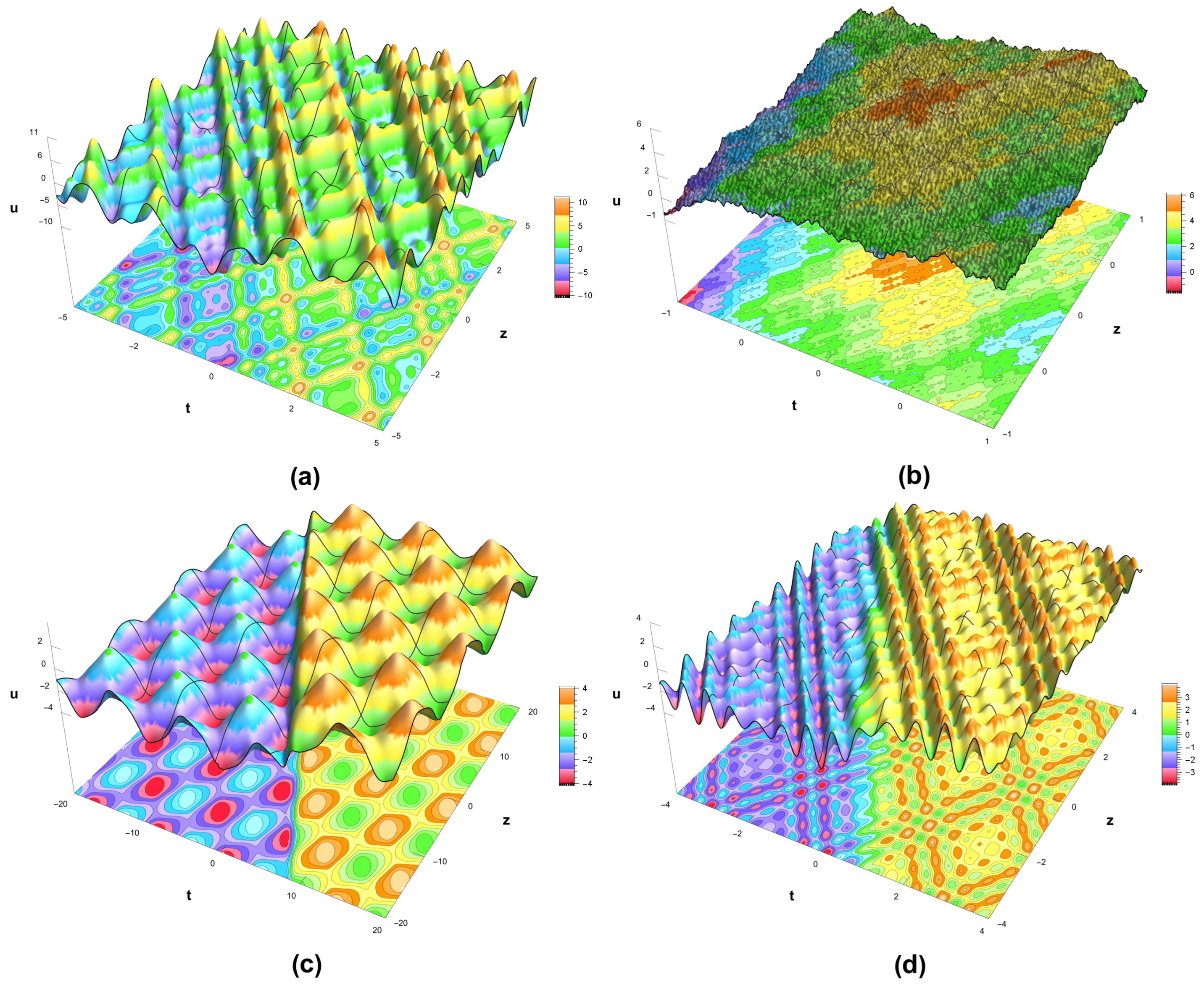
4.4. Fractal Dromion Structures via Solution $u_{13}$ (Equation (95))

Phase sine sum: A sum of $sin(ns+n^2)$ and $cos(ns+n^2)$. The quadratic phase shift $n^2$ introduces a chirp that increases with mode number, producing a highly oscillatory but localized core. Here, one gets

$$\begin{array}{cc}\hfill \mathbf{\left(}\mathbf{a}\mathbf{\right)}\mathbf{:}& f_1\left(s\right)={\displaystyle \sum _{n=1}^8}sin(ns+n^2),f_2\left(s\right)={\displaystyle \sum _{n=1}^8}cos(ns+n^2).\hfill \end{array}$$

(111)

The distinguishing feature is that the instantaneous frequency of each mode is n, but the $n^2$ phase shift causes a time-dependent interference pattern that mimics a dispersive wave packet.

Fractal butterfly: This case illustrates the high-complexity end of the localization spectrum. The dromion core is no longer a simple peak but rather a nested structure, with fluctuations repeating across multiple spatial scales. These properties are obtained by taking

$$\begin{array}{cc}\hfill \mathbf{\left(}\mathbf{b}\mathbf{\right)}\mathbf{:}& f_1\left(s\right)={\displaystyle \sum _{n=0}^{10}}0.6^{n}cos\left(3^{n}s\right),f_2\left(s\right)={\displaystyle \sum _{n=0}^{10}}0.4^{n}cos\left(5^{n}s\right).\hfill \end{array}$$

(112)

For $f_1$ with $a=0.6$, $b=3$: ${dim}_{\mathrm{box}}=2+{\displaystyle \frac{log0.6}{log3}}\approx 1.465$. For $f_2$ with $a=0.4$, $b=5$: ${dim}_{\mathrm{box}}=2+{\displaystyle \frac{log0.4}{log5}}\approx 1.431$. Numerical computation from Figure 4b yields ${dim}_{\mathrm{box}}\approx 1.44$.

Jacobi sn–cn: This construction employs the Jacobian elliptic functions sn and cn (with modulus $k=0.8$) to construct a “breathing” localized core. Unlike isolated peaks, the used dromion exhibits periodic modulation without an explicit envelope. Let us take

$$\begin{array}{cc}\hfill \mathbf{\left(}\mathbf{c}\mathbf{\right)}\mathbf{:}{f}_1\left(s\right)& =sn(s,0.8),f_2\left(s\right)=cn(s,0.8).\hfill \end{array}$$

(113)

Modulated pulse train: This dromion repeats in a regular pattern, producing coherent multi-peak structures akin to pulse trains or lattice excitations. So, one gets

$$\begin{array}{cc}\hfill \mathbf{\left(}\mathbf{d}\mathbf{\right)}\mathbf{:}{f}_1\left(s\right)& ={\displaystyle \sum _{n=-3}^3}{e}^{-{(s-3n)}^2}cos\left(10s\right),f_2\left(s\right)={\displaystyle \sum _{m=-3}^3}{e}^{-{(s-3m)}^2}sin\left(10s\right).\hfill \end{array}$$

(114)

Using Equations (111), (112), (113) and (114) together with the parameter set

$$\begin{array}{c}\hfill {\alpha }_1=0.4,{\alpha }_2=0.85,{\alpha }_3=0.3,{\alpha }_4=0.3,{\alpha }_5=0.2,{\alpha }_6=0.4,{\alpha }_7=0.2,{\alpha }_8=0.2,\mathrm{and}{c}_1=1,c_2=1,\end{array}$$

(115)

the resulting dromion solutions obtained from (95) are depicted in Figure 4.

5. Conclusions

In this work, a family of exact non-traveling wave solutions of the generalized (3 + 1)-dimensional gHSI equation is established through the application of the generalized separation of variables approach along with the mGERFM. The gHSI model serves as a unifying framework that recovers several well-known nonlinear evolution models in shallow-water wave theory, such as the Jimbo–Miwa equation, the Kadomtsev–Petviashvili equation, and the standard HSI equation. Unlike conventional traveling wave or soliton solutions that propagate with fixed speed and profile, our obtained solutions are genuinely non-traveling. They also depend on arbitrary functions of space and time, which allows them to exhibit localized, stationary, or slowly evolving behaviors. By suitably choosing these free functions, various types of dromion-like structures with fractal characteristics are derived. Such solutions provide a more reliable description of wave phenomena in inhomogeneous or time-dependent media, where classical traveling waves often fall short. The originality of the present contribution lies in the systematic integration of the generalized variable-separation technique with the mGERFM. These techniques enable us to uncover novel classes of non-traveling fractal dromion solutions in this higher-dimensional form. The presence of arbitrary functions and free parameters in the solutions offers considerable freedom to adjust the spatial and temporal structure of the waves. It is worth noting that, throughout our discussion, we have described the complex self-similar wave patterns of the solutions. Further detailed fractal analysis, including calculation of the Hausdorff dimension, verification of self-similarity using scaling relations, and examination of Hölder regularity, are beyond the scope of the present paper and are left for future studies. In summary, this work demonstrates that variable-separation methods can still be a robust and highly versatile technique to investigate interesting dynamical properties in complex nonlinear equations. In our opinion, the proposed method could be used for studying other nonlinear equations as well, leading to new opportunities for the analytical investigation of non-traveling waves in fluid mechanics, plasma physics, and nonlinear optics.