High-Precision and Robust Control of PMSM-Based Flywheel Energy Storage System Using Fractional-Order Sliding-Mode Strategy with IHAOAVOA-Based Parameter Tuning

Abstract

PMSM-based flywheel energy storage systems require fast and robust speed regulation in the presence of parameter uncertainty, load disturbances, and measurement noise, while avoiding the cost and reliability limitations associated with mechanical encoders. This paper proposes a sensorless control framework that combines a fractional-order sliding-mode speed controller with a fractional-order sliding-mode observer. To improve dynamic performance, an improved hybrid Aquila Optimizer–African Vulture Optimization Algorithm (IHAOAVOA) is employed to tune the controller parameters, while the observer follows the proposed robust sensorless design. Simulation results show that at the 1000 rpm operating point under a 20 N·m load disturbance, the proposed method limits the startup overshoot to about 0.24%, compared with 8.02% for the PI control and 9.74% for the conventional sliding-mode control. After the disturbance is introduced at $\mathrm{t}=1.0$ s, the speed drop of the proposed method is limited to 2.80%, whereas those of the PI control and conventional sliding-mode control reach 7.20% and 5.60%, respectively. At the 8000 rpm operating point under an 80 N·m load disturbance, the proposed method maintains the same advantage, with an overshoot of about 0.04% and a speed drop of 1.88%, both lower than those of the two benchmark controllers. In sensorless operation, the sensorless scheme with the IHAOAVOA-tuned speed controller also improves transient estimation performance. At the 1000 rpm operating point, the maximum startup speed estimation error is reduced from 41.8 r/min to 34.8 r/min. At the 8000 rpm operating point, the estimation error enters the ±10 r/min band at 0.0671 s, compared with 0.0718 s for the PSO-tuned case. The electromagnetic torque responses further indicate that the proposed tuning strategy improves transient torque smoothness while maintaining comparable steady-state torque behavior. These results demonstrate that the proposed control framework provides an effective balance among fast dynamic response, disturbance rejection, sensorless estimation accuracy, and electromechanical transient smoothness for PMSM-based flywheel energy storage applications.

1. Introduction

Flywheel energy storage systems (FESS) have attracted increasing attention as promising high-power and short-duration energy storage technologies because of their fast dynamic response, high power density, long service life, and high round-trip efficiency [1,2,3,4]. With the growing demand for renewable energy integration, power quality support, and rapid power balancing, FESS have been gradually extended from conventional backup-power applications to broader scenarios in modern electric energy systems [5,6].

In a practical FESS, the machine–converter set is a key subsystem because it directly determines the operating speed range, charging/discharging capability, and dynamic control performance of the whole system [7]. Among candidate electrical machines, permanent magnet synchronous motors (PMSMs), especially high-speed PMSM drives, are regarded as attractive solutions for advanced flywheel applications, owing to their high torque density, compact structure, and favorable dynamic characteristics [8,9,10]. Therefore, PMSM-based FESS have become an important research direction for high-performance flywheel systems.

Despite these advantages, PMSM-driven FESS still face several technical challenges. First, the drive system is expected to achieve accurate speed regulation over a wide operating range while maintaining robustness against parameter perturbations, load disturbances, and nonlinear effects [11]. Second, for high-speed flywheel applications, the use of mechanical position sensors is often undesirable because it may reduce reliability and increase structural complexity and maintenance burden [12]. Third, as the control framework evolves from conventional cascaded loops to advanced nonlinear and observer-based schemes, parameter tuning becomes increasingly difficult and has a strong influence on closed-loop performance.

However, most existing studies address high-performance PMSM speed regulation, sensorless estimation, and controller parameter tuning as separate problems. For PMSM-based FESS operating under high-speed and load-disturbance conditions, the coupling among speed loop robustness, observer accuracy, and tuning reproducibility has not been sufficiently investigated in a unified framework. This gap motivates the development of an integrated sensorless control strategy that combines fractional-order sliding-mode regulation, robust observation, and optimization-assisted parameter tuning.

To address these issues, this paper develops an integrated control strategy for a PMSM-based flywheel energy storage system. The proposed method combines fractional-order sliding-mode speed regulation, sensorless observation, and IHAOAVOA-based parameter tuning to improve dynamic response, suppress chattering, and enhance robustness under high-speed operation. The remainder of this paper is organized as follows. Section 2 reviews the related literature. Section 3 establishes the electromechanical model of the PMSM-driven FESS. Section 4 presents the design of the fractional-order sliding-mode controller and observer. Section 5 describes the IHAOAVOA-based controller parameter tuning method. Section 6 reports the simulation results and discussion. Section 7 summarizes the main conclusions, and Section 8 presents future work.

2. Literature Review

Recent studies related to PMSM-based flywheel energy storage can generally be grouped into three aspects: system-level FESS architecture, high-performance PMSM control, and sensorless estimation with improved parameter design.

At the system level, recent review studies have shown that FESS research has gradually evolved from a sole focus on rotor structure and bearing configuration to the coordinated design of the flywheel body, electrical machine, power converter, and control strategy [13,14,15]. In such integrated systems, the motor drive is not only responsible for bidirectional electromechanical energy conversion but also directly affects the dynamic behavior of charging/discharging processes and upper-level power regulation [16]. For applications such as renewable power smoothing and frequency support, this coordinated design requirement becomes particularly important [17].

For PMSM speed regulation, the mainstream route still starts from vector control and then introduces advanced control strategies to improve robustness and transient performance. Predictive-control-based PMSM methods have received considerable attention because they can improve response speed and reduce dependence on conventional cascaded PI tuning [18,19,20]. Disturbance-rejection-oriented methods have also been introduced into flywheel-related drive systems, particularly in cases where strong inertia, frequent state switching, and uncertain disturbances limit the performance of conventional controllers [21,22].

Sliding-mode control remains one of the most representative robust-control approaches for PMSM systems. Existing studies mainly focus on two directions. One direction is to redesign the sliding surface or reaching law so as to improve convergence characteristics and disturbance rejection [23,24]. The other direction is to reduce chattering by using disturbance observers, super-twisting structures, adaptive mechanisms, or fractional-order dynamics [25,26]. These studies indicate that improved sliding-mode methods are suitable for high-performance PMSM drives where fast speed tracking and strong robustness are simultaneously required.

Sensorless control constitutes another important branch of the literature. Since high-speed PMSM drives often avoid mechanical position sensors, observer design becomes crucial for practical implementation. Existing studies show that MRAS-based methods offer relatively simple structures and good engineering adaptability, EKF-based methods provide a model-based estimation framework but depend strongly on covariance selection and noise treatment, and sliding-mode observers remain attractive because of their robustness to parameter variations and external disturbances [27,28,29]. Nevertheless, high-speed operation, disturbance rejection, and parameter sensitivity still pose challenges for practical sensorless PMSM-based FESS.

Compared with controller design and observer design, parameter tuning is less prominent in many studies, but it has become increasingly important in practical implementation. Recent work shows a clear trend toward structured tuning and optimization-assisted parameter design for advanced nonlinear controllers and observers, with the aim of reducing empirical trial-and-error and improving the reproducibility of closed-loop performance. Therefore, integrating robust speed control, sensorless observation, and optimization-assisted parameter tuning represents a meaningful research direction for PMSM-based FESS.

Although the above studies have achieved significant progress, several issues remain open-ended. Robust speed regulation and chattering suppression are still not always addressed in a coordinated manner; high-speed sensorless estimation remains sensitive to disturbances and parameter variations; and parameter design for advanced nonlinear schemes is still often dependent on engineering experience. These issues motivate the integrated method proposed in this paper.

3. Electromechanical Model of the PMSM-Driven Flywheel Energy Storage System

This section describes the dynamic model of the PMSM-driven flywheel energy storage system adopted in this work. The model is implemented in Simulink to support controller development and performance evaluation under an ideal simulation setting. The inverter and measurement channels are assumed ideal, while electromagnetic and mechanical losses as well as thermal dynamics are neglected. Machine parameters and mechanical parameters are treated as constants. Under these assumptions, the model highlights the essential electromechanical coupling between the PMSM and the flywheel, which forms the basis for the subsequent controller and observer design [30,31,32].

From the viewpoint of energy conversion, the flywheel stores energy in the form of rotational kinetic energy, while the PMSM operates as a motor during charging and as a generator during discharging. Therefore, accurate speed regulation is directly related to the charge/discharge power capability and dynamic performance of the whole FESS. For control design, the PMSM is described in the synchronous rotating–reference frame, and the flywheel is represented through the mechanical torque–balance relationship. This modeling framework is widely adopted because it can clearly reflect the coupling among electromagnetic torque, rotor speed, and stored kinetic energy, and it is also convenient for vector control, sensorless observation, and advanced nonlinear controller design.

3.1. Flywheel Mechanical Dynamics

The energy stored in the flywheel is given by

$${\mathrm{E}}_{\mathrm{f}}={\displaystyle \frac{1}{2}}\mathrm{J}{\mathsf{\omega }}^2$$

(1)

where ${\mathrm{E}}_{\mathrm{f}}$ is the flywheel kinetic energy, $\mathrm{J}$ is the equivalent moment of inertia of the rotor system, and $\mathsf{\omega }$ denotes the mechanical angular speed. As indicated by (1), the stored energy increases quadratically with the rotational speed. This implies that speed regulation is directly related to the energy conversion capability of the flywheel energy storage system.

The mechanical dynamics of the PMSM–flywheel set can be described by the torque equilibrium equation

$$\mathrm{J}\dot{\mathsf{\omega }}={\mathrm{T}}_{\mathrm{e}}-{\mathrm{T}}_{\mathrm{L}}-\mathrm{B}\mathsf{\omega }$$

(2)

where ${\mathrm{T}}_{\mathrm{e}}$ is the electromagnetic torque produced by the PMSM, ${\mathrm{T}}_{\mathrm{L}}$ is the external load/disturbance torque, $\mathrm{B}$ is the viscous friction coefficient, and $\mathrm{B}\mathsf{\omega }$ denotes the viscous damping torque. According to (2), the rotor speed changes when the electromagnetic torque is not balanced by the resisting torque. Hence, the mechanical speed of the flywheel can be controlled by regulating ${\mathrm{T}}_{\mathrm{e}}$, while the disturbance torque and friction torque act as factors that degrade dynamic performance.

During charging, the PMSM accelerates the flywheel and converts electrical energy into mechanical kinetic energy. During discharging, the flywheel decelerates and the stored kinetic energy is converted back into electrical energy through the PMSM. Therefore, (1) and (2) establish the fundamental mechanical model for describing the bidirectional energy conversion process of the FESS.

3.2. PMSM Model in the $d$–$q$ Reference Frame

For controller design, the electrical dynamics of the PMSM are expressed in the synchronous rotating $\mathrm{d}$–$\mathrm{q}$ reference frame as

$$\begin{array}{c}{\mathrm{v}}_{\mathrm{d}}={\mathrm{R}}_{\mathrm{s}}{\mathrm{i}}_{\mathrm{d}}+{\mathrm{L}}_{\mathrm{d}}{\dot{\mathrm{i}}}_{\mathrm{d}}-{\mathsf{\omega }}_{\mathrm{e}}{\mathrm{L}}_{\mathrm{q}}{\mathrm{i}}_{\mathrm{q}},\\ {\mathrm{v}}_{\mathrm{q}}={\mathrm{R}}_{\mathrm{s}}{\mathrm{i}}_{\mathrm{q}}+{\mathrm{L}}_{\mathrm{q}}{\dot{\mathrm{i}}}_{\mathrm{q}}+{\mathsf{\omega }}_{\mathrm{e}}\left({\mathrm{L}}_{\mathrm{d}}{\mathrm{i}}_{\mathrm{d}}+{\mathsf{\psi }}_{\mathrm{f}}\right)\end{array}$$

(3)

where ${\mathrm{v}}_{\mathrm{d}}$ and ${\mathrm{v}}_{\mathrm{q}}$ denote the $\mathrm{d}$- and $\mathrm{q}$-axis stator voltages, ${\mathrm{i}}_{\mathrm{d}}$ and ${\mathrm{i}}_{\mathrm{q}}$ denote the corresponding stator currents, ${\mathrm{R}}_{\mathrm{s}}$ is the stator resistance, ${\mathrm{L}}_{\mathrm{d}}$ and ${\mathrm{L}}_{\mathrm{q}}$ are the $\mathrm{d}$- and $\mathrm{q}$-axis inductances, ${\mathsf{\psi }}_{\mathrm{f}}$ is the permanent-magnet flux linkage, and ${\mathsf{\omega }}_{\mathrm{e}}$ is the electrical angular speed. The first two terms on the right-hand side of each equation represent the resistive and inductive voltage drops, whereas the speed-dependent terms describe the cross-coupling effect between the two axes. Therefore, (3) characterizes the electrical dynamic behavior of the PMSM in the rotating reference frame.

The electromagnetic torque is given by

$${\mathrm{T}}_{\mathrm{e}}={\displaystyle \frac{3}{2}}\mathrm{p}\left({\mathsf{\psi }}_{\mathrm{f}}{\mathrm{i}}_{\mathrm{q}}+({\mathrm{L}}_{\mathrm{d}}-{\mathrm{L}}_{\mathrm{q}}){\mathrm{i}}_{\mathrm{d}}{\mathrm{i}}_{\mathrm{q}}\right)$$

(4)

where ${\mathrm{T}}_{\mathrm{e}}$ is the electromagnetic torque and $\mathrm{p}$ is the pole-pair number. As shown in (4), the developed torque consists of a permanent-magnet torque component and a reluctance torque component. For surface-mounted PMSMs, commonly employed in high-speed flywheel systems, the rotor saliency is usually weak and the inductances satisfy ${\mathrm{L}}_{\mathrm{d}}\approx {\mathrm{L}}_{\mathrm{q}}$. Accordingly, the reluctance torque term can be neglected, and (4) is simplified to

$${\mathrm{T}}_{\mathrm{e}}\approx {\displaystyle \frac{3}{2}}\mathrm{p}{\mathsf{\psi }}_{\mathrm{f}}{\mathrm{i}}_{\mathrm{q}}$$

(5)

Equation (5) indicates that the electromagnetic torque is approximately proportional to the $\mathrm{q}$-axis current. This property is beneficial for decoupled control design, since the $\mathrm{q}$-axis current can be directly used as the main torque regulation variable in the PMSM-driven FESS.

3.3. Electromechanical Coupling and Operational Constraints

By combining the mechanical model in (2) with the electromagnetic torque relationship in (5), the PMSM-driven FESS can be represented by a compact electromechanical coupling structure. In this structure, the $\mathrm{q}$-axis current determines the electromagnetic torque, the torque governs the rotor speed variation, and the rotor speed further determines the stored kinetic energy. Hence, the energy-conversion process of the system can be described by the relationship from current to torque, from torque to speed, and from speed to stored energy.

For the surface-mounted PMSM considered in this work, the torque is approximately proportional to ${\mathrm{i}}_{\mathrm{q}}$. Therefore, the $\mathrm{q}$-axis current serves as the main control input for torque and speed regulation, which provides a clear basis for the subsequent controller design.

Meanwhile, the system operation must satisfy several practical constraints. The stator current is limited by the current rating of the machine and converter,

$${\mathrm{i}}_{\mathrm{d}}^2+{\mathrm{i}}_{\mathrm{q}}^2\le {\mathrm{I}}_{\mathrm{m}\mathrm{a}\mathrm{x}}^2$$

(6)

the stator voltage is limited by the inverter output capability,

$${\mathrm{v}}_{\mathrm{d}}^2+{\mathrm{v}}_{\mathrm{q}}^2\le {\mathrm{V}}_{\mathrm{m}\mathrm{a}\mathrm{x}}^2$$

(7)

and the flywheel speed must remain within the permissible operating range,

$${\mathsf{\omega }}_{\mathrm{m}\mathrm{i}\mathrm{n}}\le \mathsf{\omega }\le {\mathsf{\omega }}_{\mathrm{m}\mathrm{a}\mathrm{x}}$$

(8)

These bounds define the feasible operating region of the PMSM-driven FESS. In the Simulink model, they are imposed as ideal operational limits to reflect the machine and inverter ratings under the adopted simplified assumptions.

4. Fractional-Order Sliding-Mode Control and Observer Design

In practical operating conditions, the PMSM-based flywheel energy storage system is subject to parameter perturbations, load disturbances, and sensorless operation requirements, which make accurate speed regulation and state estimation difficult to achieve simultaneously. In particular, external disturbances and model uncertainties may deteriorate the dynamic response of the speed loop, while the absence of a mechanical position sensor increases the dependence of the control system on the estimation accuracy of rotor speed and position.

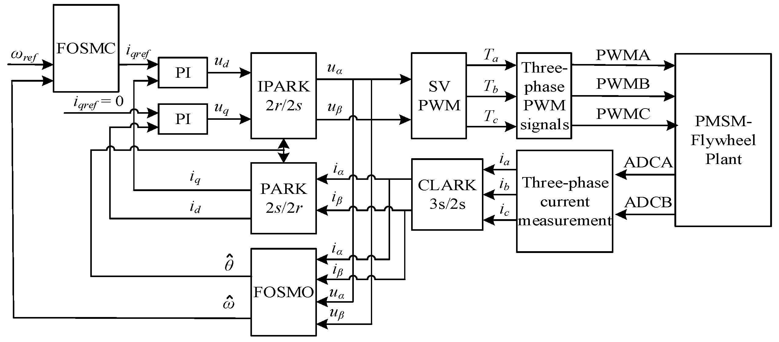
To address these issues, a fractional-order sliding-mode control scheme with sensorless observation is developed in this work, and its key controller parameters are subsequently optimized using IHAOAVOA. The proposed method employs a fractional-order sliding-mode controller to enhance the robustness and dynamic performance of the outer speed loop, while a fractional-order sliding-mode observer is introduced to estimate the rotor speed and position required for sensorless operation. Meanwhile, inner current loops are implemented in the synchronous rotating reference frame, and inverter switching signals are generated through the inverse Park transformation and space-vector pulse width modulation.

The overall sensorless control structure of the proposed PMSM-driven FESS is shown in Figure 1.

4.1. Improved Fractional-Order Sliding-Mode Control Design

For the PMSM-driven flywheel energy storage system, a speed loop is required to maintain fast response and strong robustness under parameter perturbations and load disturbances. Conventional sliding-mode control provides satisfactory robustness, but its dynamic behavior is often affected by chattering and limited tuning flexibility. To improve the transient response and enhance the regulation capability of the speed loop, an improved fractional-order sliding-mode controller (FOSMC) is adopted in this work. By introducing a fractional-order operator into the sliding surface and combining it with a nonlinear reaching law, the proposed controller aims to achieve faster convergence and smoother control action for flywheel speed regulation.

4.1.1. Speed Tracking Error and Fractional-Order Sliding Surface

The speed tracking error is defined as

$${\mathrm{e}}_{\mathsf{\omega }}={\mathsf{\omega }}_{\mathrm{r}\mathrm{e}\mathrm{f}}-\mathsf{\omega }$$

(9)

where ${\mathsf{\omega }}_{\mathrm{r}\mathrm{e}\mathrm{f}}$ is the reference speed and $\mathsf{\omega }$ is the actual rotor speed. Therefore, ${\mathrm{e}}_{\mathsf{\omega }}$ represents the deviation of the flywheel speed from its desired operating point and serves as the basic state variable for the speed controller.

In this work, the fractional-order operators are implemented using the FOMCON-based Oustaloup recursive approximation. The detailed numerical implementation settings are provided in Section 6.1. Based on the speed tracking error in Equation (9), the fractional-order sliding surface used in this work is constructed as

$$\mathrm{s}={\mathrm{e}}_{\mathsf{\omega }}+{\mathrm{D}}^{-0.8}\left(\mathrm{c}{\mathrm{e}}_{\mathsf{\omega }}\right)$$

(10)

where $\mathrm{s}$ denotes the sliding variable, $\mathrm{c}$ is the coefficient of the fractional integral term, and ${\mathrm{D}}^{-0.8}$ represents the fractional-order integral operator with order 0.8. In this structure, the first term reflects the instantaneous speed tracking error, while the second term introduces the memory effect of the historical speed error through the fractional-order integral channel. Therefore, the sliding surface combines the present error information and the memory-dependent accumulated error information.

When the system trajectory reaches the sliding manifold, $\mathrm{s}=0$, Equation (10) gives

$${\mathrm{e}}_{\mathsf{\omega }}+{\mathrm{D}}^{-0.8}\left(\mathrm{c}{\mathrm{e}}_{\mathsf{\omega }}\right)=0$$

(11)

Applying the fractional operator ${\mathrm{D}}^{0.8}$ to both sides yields the equivalent fractional-order error dynamic

$${\mathrm{D}}^{0.8}{\mathrm{e}}_{\mathsf{\omega }}+\mathrm{c}{\mathrm{e}}_{\mathsf{\omega }}=0$$

(12)

For $\mathrm{c}>0$, this fractional-order error equation provides an asymptotically convergent sliding motion. Therefore, the fractional-order term does not merely act as an additional integral correction; it shapes the memory-dependent convergence behavior of the speed tracking error. The coefficient $\mathrm{c}$ determines the weight of the fractional integral term, while the fixed order 0.8 determines the memory depth adopted in the FOMCON implementation.

4.1.2. Torque-Equivalent Reaching Command

To generate the torque-equivalent command for the outer speed loop, the sliding variable in Equation (10) is combined with a switching term and a proportional error-compensation term. The torque-equivalent command is expressed as

$${\mathrm{T}}_{\mathrm{c}\mathrm{m}\mathrm{d}}=\mathrm{q}\mathrm{s}+\mathsf{\mu }\mathrm{s}\mathrm{g}\mathrm{n}(\mathrm{s})+{\mathrm{k}}_{\mathrm{e}}{\mathrm{e}}_{\mathsf{\omega }}+{\widehat{\mathrm{T}}}_{\mathrm{L}}$$

(13)

where ${\mathrm{T}}_{\mathrm{c}\mathrm{m}\mathrm{d}}$ is the torque-equivalent command generated by the speed controller, $\mathrm{q}$ is the coefficient of the sliding variable term, $\mathsf{\mu }$ is the switching gain, ${\mathrm{k}}_{\mathrm{e}}$ is the proportional compensation gain of the speed error, and ${\widehat{\mathrm{T}}}_{\mathrm{L}}$ denotes the available load torque compensation term. The term $\mathrm{q}\mathrm{s}$ provides a continuous correction along the sliding variable, $\mathsf{\mu }\mathrm{s}\mathrm{g}\mathrm{n}\left(\mathrm{s}\right)$ strengthens robustness against disturbance and uncertainty, and ${\mathrm{k}}_{\mathrm{e}}{\mathrm{e}}_{\mathsf{\omega }}$ improves the direct speed-error correction capability. In this way, Equation (13) combines fractional-order sliding information, switching robustness, and proportional speed-error compensation.

4.1.3. Current-Reference Generation

For the surface-mounted PMSM considered in this work, the electromagnetic torque is approximately proportional to the q-axis current, as established in Section 3, as follows:

$${\mathrm{T}}_{\mathrm{e}}=1.5\mathrm{p}{\mathsf{\psi }}_{\mathrm{f}}{\mathrm{i}}_{\mathrm{q}}$$

(14)

Therefore, after the torque-equivalent command ${\mathrm{T}}_{\mathrm{c}\mathrm{m}\mathrm{d}}$ is generated by Equation (13), the corresponding q-axis current reference can be obtained from the torque–current relationship as

$${\mathrm{i}}_{\mathrm{q}}^{\mathrm{r}\mathrm{e}\mathrm{f}}={\mathrm{s}\mathrm{a}\mathrm{t}}_{[-{\mathrm{I}}_{\mathrm{m}\mathrm{a}\mathrm{x}},{\mathrm{I}}_{\mathrm{m}\mathrm{a}\mathrm{x}}]}\left({\displaystyle \frac{{\mathrm{T}}_{\mathrm{c}\mathrm{m}\mathrm{d}}}{1.5\mathrm{p}{\mathsf{\psi }}_{\mathrm{f}}}}\right)$$

(15)

Here, ${\mathrm{i}}_{\mathrm{q}}^{\mathrm{r}\mathrm{e}\mathrm{f}}$ is the q-axis current reference, $\mathrm{p}$ is the pole-pair number, ${\mathsf{\psi }}_{\mathrm{f}}$ is the permanent-magnet flux linkage, and ${\mathrm{I}}_{\mathrm{m}\mathrm{a}\mathrm{x}}$ is the allowable current limit. In the Simulink implementation, ${\mathrm{I}}_{\mathrm{m}\mathrm{a}\mathrm{x}}=160$ A. Equation (15) shows that the output of the FOSMC speed loop is first formed as a torque-equivalent command and then converted into the q-axis current reference required by the inner current loop. In this way, the proposed controller is consistent with the PMSM torque-generation mechanism while preserving the robustness provided by the sliding-mode command in Equation (13).

4.1.4. Stability Interpretation

To explain the stability-related role of the proposed sliding surface and reaching command, consider the Lyapunov candidate function

$$\mathrm{V}={\displaystyle \frac{1}{2}}{\mathrm{s}}^2$$

(16)

For the ideal current-tracking case, the torque-equivalent command in Equation (13) drives the sliding variable toward the sliding manifold through the continuous correction term $\mathrm{q}\mathrm{s}$ and the switching term $\mathsf{\mu }\mathrm{s}\mathrm{g}\mathrm{n}\left(\mathrm{s}\right)$. The equivalent reaching behavior can be expressed in the form

$$\dot{\mathrm{s}}=-\mathrm{q}\mathrm{s}-\mathsf{\mu }\mathrm{s}\mathrm{g}\mathrm{n}\left(\mathrm{s}\right)+{\mathrm{d}}_{\mathrm{s}}$$

(17)

where ${\mathrm{d}}_{\mathrm{s}}$ denotes the bounded lumped effect of model mismatch, disturbance estimation error, and inner-loop tracking error. Taking the derivative of $\mathrm{V}$ gives

$$\dot{\mathrm{V}}=\mathrm{s}\dot{\mathrm{s}}=-\mathrm{q}{\mathrm{s}}^2-\mathsf{\mu }|\mathrm{s}|+\mathrm{s}{\mathrm{d}}_{\mathrm{s}}$$

(18)

If $\left|{\mathrm{d}}_{\mathrm{s}}\right|\le {\mathrm{d}}_{\mathrm{m}\mathrm{a}\mathrm{x}}$ and $\mathsf{\mu }>{\mathrm{d}}_{\mathrm{m}\mathrm{a}\mathrm{x}}$, then

$$\dot{\mathrm{V}}\le -\mathrm{q}{\mathrm{s}}^2-(\mathsf{\mu }-{\mathrm{d}}_{\mathrm{m}\mathrm{a}\mathrm{x}})|\mathrm{s}|\le 0$$

(19)

Therefore, the sliding variable remains bounded and is driven toward the sliding manifold. Once the sliding motion is established, Equation (10) leads to the fractional-order error dynamics ${\mathrm{D}}^{0.8}{\mathrm{e}}_{\mathsf{\omega }}+\mathrm{c}{\mathrm{e}}_{\mathsf{\omega }}=0$, which provides the convergence basis for the speed tracking error. This analysis indicates that the proposed FOSMC structure combines memory-dependent error convergence with sliding-mode robustness against bounded disturbances.

4.2. Fractional-Order Sliding-Mode Observer Design

For the PMSM-driven flywheel energy storage system, sensorless operation requires accurate estimation of rotor position and speed without using a mechanical encoder. However, parameter variations, measurement noise, and unmodeled disturbances may degrade the estimation performance of conventional observers, especially under high-speed operating conditions. To improve the robustness and dynamic accuracy of state estimation, a fractional-order sliding-mode observer (FOSMO) is developed in this work. By introducing a fractional-order injection term into the observer structure, the proposed method enhances disturbance rejection while preserving the advantages of sliding-mode-based estimation.

4.2.1. PMSM Model in the Stationary $\mathsf{\alpha }$–$\mathsf{\beta }$ Frame

For the observer design, the PMSM electrical model is expressed in the stationary $\mathsf{\alpha }$–$\mathsf{\beta }$ reference frame as

$$\begin{array}{c}{\displaystyle \frac{\mathrm{d}{\mathrm{i}}_{\mathsf{\alpha }}}{\mathrm{d}\mathrm{t}}}=-{\displaystyle \frac{{\mathrm{R}}_{\mathrm{s}}}{{\mathrm{L}}_{\mathrm{s}}}}{\mathrm{i}}_{\mathsf{\alpha }}+{\displaystyle \frac{1}{{\mathrm{L}}_{\mathrm{s}}}}{\mathrm{v}}_{\mathsf{\alpha }}-{\displaystyle \frac{{\mathsf{\psi }}_{\mathrm{f}}}{{\mathrm{L}}_{\mathrm{s}}}}{\mathsf{\omega }}_{\mathrm{e}}\mathrm{s}\mathrm{i}\mathrm{n}{\mathsf{\theta }}_{\mathrm{e}}\\ {\displaystyle \frac{\mathrm{d}{\mathrm{i}}_{\mathsf{\beta }}}{\mathrm{d}\mathrm{t}}}=-{\displaystyle \frac{{\mathrm{R}}_{\mathrm{s}}}{{\mathrm{L}}_{\mathrm{s}}}}{\mathrm{i}}_{\mathsf{\beta }}+{\displaystyle \frac{1}{{\mathrm{L}}_{\mathrm{s}}}}{\mathrm{v}}_{\mathsf{\beta }}+{\displaystyle \frac{{\mathsf{\psi }}_{\mathrm{f}}}{{\mathrm{L}}_{\mathrm{s}}}}{\mathsf{\omega }}_{\mathrm{e}}\mathrm{c}\mathrm{o}\mathrm{s}{\mathsf{\theta }}_{\mathrm{e}}\end{array}$$

(20)

where ${\mathrm{i}}_{\mathsf{\alpha }}$ and ${\mathrm{i}}_{\mathsf{\beta }}$ are the stator currents in the stationary reference frame, ${\mathrm{v}}_{\mathsf{\alpha }}$ and ${\mathrm{v}}_{\mathsf{\beta }}$ are the corresponding stator voltages, ${\mathrm{R}}_{\mathrm{s}}$ is the stator resistance, ${\mathrm{L}}_{\mathrm{s}}$ is the stator inductance, ${\mathsf{\psi }}_{\mathrm{f}}$ is the permanent-magnet flux linkage, ${\mathsf{\omega }}_{\mathrm{e}}$ is the electrical angular speed, and ${\mathsf{\theta }}_{\mathrm{e}}$ is the electrical rotor position. The first term on the right-hand side of each equation represents the resistive voltage drop, the second term describes the input voltage effect, and the last term corresponds to the back-EMF component induced by rotor motion. Therefore, (20) provides the basic current dynamic model from which the rotor position and speed can be estimated.

4.2.2. FOSMO Structure with Fractional Injection

Based on the stationary-frame current model in Equation (20), the current-estimation errors are defined as

$${\mathrm{e}}_{\mathsf{\alpha }}={\mathrm{i}}_{\mathsf{\alpha }}-{\widehat{\mathrm{i}}}_{\mathsf{\alpha }}, {\mathrm{e}}_{\mathsf{\beta }}={\mathrm{i}}_{\mathsf{\beta }}-{\widehat{\mathrm{i}}}_{\mathsf{\beta }}$$

(21)

The observer implemented in this work can be expressed as

$$\begin{array}{c}{\displaystyle \frac{\mathrm{d}{\widehat{\mathrm{i}}}_{\mathsf{\alpha }}}{\mathrm{d}\mathrm{t}}}={\displaystyle \frac{{\mathrm{u}}_{\mathsf{\alpha }}-{\mathrm{R}}_{\mathrm{s}}{\widehat{\mathrm{i}}}_{\mathsf{\alpha }}-{\mathrm{E}}_{\mathsf{\alpha }}}{{\mathrm{L}}_{\mathrm{s}}}},\\ {\displaystyle \frac{\mathrm{d}{\widehat{\mathrm{i}}}_{\mathsf{\beta }}}{\mathrm{d}\mathrm{t}}}={\displaystyle \frac{{\mathrm{u}}_{\mathsf{\beta }}-{\mathrm{R}}_{\mathrm{s}}{\widehat{\mathrm{i}}}_{\mathsf{\beta }}-{\mathrm{E}}_{\mathsf{\beta }}}{{\mathrm{L}}_{\mathrm{s}}}} \end{array}$$

(22)

where ${\mathrm{L}}_{\mathrm{s}}={\mathrm{L}}_{\mathrm{d}}={\mathrm{L}}_{\mathrm{q}}$ for the surface-mounted PMSM, ${\widehat{\mathrm{i}}}_{\mathsf{\alpha }}$ and ${\widehat{\mathrm{i}}}_{\mathsf{\beta }}$ are the estimated stator currents, ${\mathrm{u}}_{\mathsf{\alpha }}$ and ${\mathrm{u}}_{\mathsf{\beta }}$ are the stationary-frame voltage inputs, and ${\mathrm{E}}_{\mathsf{\alpha }}$ and ${\mathrm{E}}_{\mathsf{\beta }}$ are the equivalent back-EMF estimation and correction terms generated by the fractional-order sliding-mode observer. For each stationary-frame axis $\mathrm{x}\in \{\mathsf{\alpha },\mathsf{\beta }\}$, the fractional sliding variable of the observer is written as

$${\mathsf{\sigma }}_{\mathrm{x}}={\mathrm{e}}_{\mathrm{x}}+{\mathrm{D}}^{-0.98}\left({\mathsf{\lambda }}_{\mathrm{o}}{\mathrm{e}}_{\mathrm{x}}\right)$$

(23)

and the corresponding correction term is constructed as

$${\mathrm{E}}_{\mathrm{x}}=\mathsf{\eta }{\mathsf{\sigma }}_{\mathrm{x}}+{\mathsf{\mu }}_{\mathrm{o}}\mathrm{s}\mathrm{g}\mathrm{n}\left({\mathsf{\sigma }}_{\mathrm{x}}\right)+{\mathrm{D}}^{-1.98}\left({\mathsf{\lambda }}_1{\mathrm{e}}_{\mathrm{x}}\right)$$

(24)

In the implementation, ${\mathsf{\lambda }}_{\mathrm{o}}=5634.4$, ${\mathsf{\lambda }}_1=5634.4{\mathrm{L}}_{\mathrm{s}}$, ${\mathsf{\mu }}_{\mathrm{o}}=-0.001$, and $\mathsf{\eta }=-10.722$. The fractional-order operators in the observer are implemented by the FOMCON-based Oustaloup recursive approximation. Compared with a conventional sliding-mode observer, the fractional-order correction introduces memory-dependent information into the injection channel, which improves the flexibility of observer tuning and enhances the robustness of sensorless estimation.

4.2.3. Back-EMF Extraction and Rotor Position/Speed Estimation

After the observer reaches the sliding regime, the equivalent correction terms ${\mathrm{E}}_{\mathsf{\alpha }}$ and ${\mathrm{E}}_{\mathsf{\beta }}$ contain the reconstructed back-EMF information. Therefore, the estimated back-EMF components are obtained as

$$\begin{array}{c}{\widehat{\mathrm{e}}}_{\mathsf{\alpha }}\approx {\mathrm{E}}_{\mathsf{\alpha }},\\ {\widehat{\mathrm{e}}}_{\mathsf{\beta }}\approx {\mathrm{E}}_{\mathsf{\beta }}\end{array}$$

(25)

For the surface-mounted PMSM, the stationary-frame back-EMF components satisfy

$$\begin{array}{c}{\mathrm{e}}_{\mathsf{\alpha }}=-{\mathsf{\psi }}_{\mathrm{f}}{\mathsf{\omega }}_{\mathrm{e}}\mathrm{s}\mathrm{i}\mathrm{n}{\mathsf{\theta }}_{\mathrm{e}},\\ {\mathrm{e}}_{\mathsf{\beta }}={\mathsf{\psi }}_{\mathrm{f}}{\mathsf{\omega }}_{\mathrm{e}}\mathrm{c}\mathrm{o}\mathrm{s}{\mathsf{\theta }}_{\mathrm{e}}.\end{array}$$

(26)

Therefore, the electrical rotor position can be reconstructed from the orientation of the back-EMF vector as

$${\widehat{\mathsf{\theta }}}_{\mathrm{e}}=\mathrm{a}\mathrm{t}\mathrm{a}\mathrm{n}2(-{\widehat{\mathrm{e}}}_{\mathsf{\alpha }},{\widehat{\mathrm{e}}}_{\mathsf{\beta }})$$

(27)

and the electrical angular speed is obtained by differentiating the estimated rotor position as follows:

$${\widehat{\mathsf{\omega }}}_{\mathrm{e}}={\displaystyle \frac{\mathrm{d}{\widehat{\mathsf{\theta }}}_{\mathrm{e}}}{\mathrm{d}\mathrm{t}}}$$

(28)

The use of the atan2 operator avoids quadrant ambiguity in conventional arctangent calculation and improves the robustness of angle reconstruction. In practical implementation, the differentiated angle signal is filtered to suppress high-frequency noise amplification. Therefore, once the back-EMF vector is reconstructed, the rotor angle and speed can be obtained in a physically consistent manner.

4.2.4. Adaptive Boundary Layer for Noise Mitigation

To reduce the influence of high-frequency switching noise and measurement ripple, an adaptive boundary layer treatment is introduced for the discontinuous injection term as follows:

$$D^{-0.98}\mathrm{s}\mathrm{g}\mathrm{n}(e_x)\approx \left\{\begin{array}{ll}{D}^{-0.98}\left({\displaystyle \frac{e_x}{\mathsf{\Phi }}}\right),& \left|e_x\right|\le \mathsf{\Phi }\\ D^{-0.98}\mathrm{s}\mathrm{g}\mathrm{n}\left(e_x\right),& otherwise\end{array}\right.$$

(29)

where $\mathrm{x}\in \{\mathsf{\alpha },\mathsf{\beta }\}$, $e_x$ is the corresponding current-estimation error, and $\mathsf{\Phi }$ is the boundary layer thickness. Within the boundary layer, the discontinuous sign function is replaced by a continuous approximation, which weakens chattering and reduces noise amplification near the sliding surface. Outside the boundary layer, the original discontinuous term is retained to preserve the fast convergence property of sliding-mode estimation.

To improve adaptability under different operating conditions, the boundary layer thickness is updated as

$$\mathsf{\Phi }={\mathsf{\Phi }}_0+{\mathsf{\Phi }}_1\parallel \mathrm{e}\parallel$$

(30)

where ${\mathsf{\Phi }}_0>0$ and ${\mathsf{\Phi }}_1>0$ are design coefficients, and $\mathrm{e}=[{\mathrm{e}}_{\mathsf{\alpha }},{\mathrm{e}}_{\mathsf{\beta }}{]}^{\mathrm{T}}$ is the current-estimation error vector. Equation (30) implies that the boundary layer becomes wider when the estimation error is large, which helps suppress excessive switching and improve noise tolerance during transient conditions. As the error decreases, the boundary layer is correspondingly reduced, thereby preserving estimation precision in steady-state operation.

4.2.5. Lyapunov Stability of the Observer

To clarify the convergence mechanism of the observer, the stability analysis is established for the ideal equivalent sliding-mode injection term. The practical FOMCON-based fractional correction in Equations (23) and (24) is used in simulation, while the equivalent injection form is used here to explain the convergence of the estimation error.

For $\mathrm{x}\in \{\mathsf{\alpha },\mathsf{\beta }\}$, the current-estimation error is defined as

$${\mathrm{e}}_{\mathrm{x}}={\mathrm{i}}_{\mathrm{x}}-{\widehat{\mathrm{i}}}_{\mathrm{x}}$$

(31)

The corresponding idealized error dynamics can be written as

$${\dot{\mathrm{e}}}_{\mathrm{x}}=-{\displaystyle \frac{{\mathrm{R}}_{\mathrm{s}}}{{\mathrm{L}}_{\mathrm{s}}}}{\mathrm{e}}_{\mathrm{x}}+{\displaystyle \frac{1}{{\mathrm{L}}_{\mathrm{s}}}}\left({\mathrm{e}}_{\mathrm{x},\mathrm{e}\mathrm{m}\mathrm{f}}-{\mathrm{K}}_{\mathrm{o}}\mathrm{s}\mathrm{g}\mathrm{n}\left({\mathrm{e}}_{\mathrm{x}}\right)\right)$$

(32)

where ${\mathrm{e}}_{\mathrm{x},\mathrm{e}\mathrm{m}\mathrm{f}}$ denotes the corresponding back-EMF component and ${\mathrm{K}}_{\mathrm{o}}$ is the equivalent observer injection gain. Consider the Lyapunov candidate function

$${\mathrm{V}}_{\mathrm{o}}={\displaystyle \frac{1}{2}}({\mathrm{e}}_{\mathsf{\alpha }}^2+{\mathrm{e}}_{\mathsf{\beta }}^2)$$

(33)

Taking the derivative of ${\mathrm{V}}_{\mathrm{o}}$ along the error dynamics gives

$$\begin{array}{c}{\dot{\mathrm{V}}}_{\mathrm{o}}={\mathrm{e}}_{\mathsf{\alpha }}{\dot{\mathrm{e}}}_{\mathsf{\alpha }}+{\mathrm{e}}_{\mathsf{\beta }}{\dot{\mathrm{e}}}_{\mathsf{\beta }}\\ =-{\displaystyle \frac{{\mathrm{R}}_{\mathrm{s}}}{{\mathrm{L}}_{\mathrm{s}}}}({\mathrm{e}}_{\mathsf{\alpha }}^2+{\mathrm{e}}_{\mathsf{\beta }}^2)+{\displaystyle \frac{1}{{\mathrm{L}}_{\mathrm{s}}}}({\mathrm{e}}_{\mathsf{\alpha }}{\mathrm{e}}_{\mathsf{\alpha },\mathrm{e}\mathrm{m}\mathrm{f}}+{\mathrm{e}}_{\mathsf{\beta }}{\mathrm{e}}_{\mathsf{\beta },\mathrm{e}\mathrm{m}\mathrm{f}})-{\displaystyle \frac{{\mathrm{K}}_{\mathrm{o}}}{{\mathrm{L}}_{\mathrm{s}}}}(|{\mathrm{e}}_{\mathsf{\alpha }}|+|{\mathrm{e}}_{\mathsf{\beta }}|)\end{array}$$

(34)

If the back-EMF components are bounded by $\left|{\mathrm{e}}_{\mathrm{x},\mathrm{e}\mathrm{m}\mathrm{f}}\right|\le {\mathrm{E}}_{\mathrm{m}\mathrm{a}\mathrm{x}}$ and the equivalent observer gain satisfies ${\mathrm{K}}_{\mathrm{o}}>{\mathrm{E}}_{\mathrm{m}\mathrm{a}\mathrm{x}}$, then

$${\dot{\mathrm{V}}}_{\mathrm{o}}\le -{\displaystyle \frac{{\mathrm{R}}_{\mathrm{s}}}{{\mathrm{L}}_{\mathrm{s}}}}\parallel \mathrm{e}{\parallel }^2-{\displaystyle \frac{{\mathrm{K}}_{\mathrm{o}}-{\mathrm{E}}_{\mathrm{m}\mathrm{a}\mathrm{x}}}{{\mathrm{L}}_{\mathrm{s}}}}(|{\mathrm{e}}_{\mathsf{\alpha }}|+|{\mathrm{e}}_{\mathsf{\beta }}|)\le 0$$

(35)

Equation (35) shows explicitly how the right-hand side is obtained from the Lyapunov derivative. The resistive term provides damping, the bounded back-EMF term is compensated by the observer injection gain, and the remaining negative term drives the current-estimation errors toward the sliding region. Therefore, the observer states remain bounded, and the reconstructed back-EMF signals can be used for rotor position and speed estimation.

4.3. Sensorless Integration and Implementation in Simulink

The proposed sensorless control scheme is implemented by integrating the FOSMC speed controller and the FOSMO within a standard cascaded control structure. In this closed-loop framework, the observer provides the estimated electrical rotor position ${\widehat{\mathsf{\theta }}}_{\mathrm{e}}$ and speed ${\widehat{\mathsf{\omega }}}_{\mathrm{e}}$, which are used for coordinate transformation and speed feedback, respectively. In this way, the PMSM-driven FESS can operate without a mechanical position sensor while maintaining the signal consistency required by the controller.

Specifically, the measured three-phase stator currents are first transformed into the stationary $\mathsf{\alpha }$–$\mathsf{\beta }$ frame and then mapped into the synchronous rotating $\mathrm{d}$–$\mathrm{q}$ frame by using the estimated rotor angle. The corresponding current transformation is given by

$$\left[\begin{array}{c}{\mathrm{i}}_{\mathrm{d}}\\ {\mathrm{i}}_{\mathrm{q}}\end{array}\right]=\left[\begin{array}{cc}\mathrm{c}\mathrm{o}\mathrm{s}{\widehat{\mathsf{\theta }}}_{\mathrm{e}}& \mathrm{s}\mathrm{i}\mathrm{n}{\widehat{\mathsf{\theta }}}_{\mathrm{e}}\\ -\mathrm{s}\mathrm{i}\mathrm{n}{\widehat{\mathsf{\theta }}}_{\mathrm{e}}& \mathrm{c}\mathrm{o}\mathrm{s}{\widehat{\mathsf{\theta }}}_{\mathrm{e}}\end{array}\right]\left[\begin{array}{c}{\mathrm{i}}_{\mathsf{\alpha }}\\ {\mathrm{i}}_{\mathsf{\beta }}\end{array}\right]$$

(36)

where ${\mathrm{i}}_{\mathsf{\alpha }}$ and ${\mathrm{i}}_{\mathsf{\beta }}$ are the stator currents in the stationary reference frame, and ${\mathrm{i}}_{\mathrm{d}}$ and ${\mathrm{i}}_{\mathrm{q}}$ are the corresponding current components in the synchronous rotating reference frame. Equation (36) shows that the estimated angle supplied by the observer directly determines the coordinate alignment used in current regulation and speed control.

Based on the estimated speed feedback, the outer-loop FOSMC generates the control command for speed regulation, while the $\mathrm{d}$-axis reference is set according to the operating policy of the surface-mounted PMSM. Under the ideal operating condition considered in this work, the $\mathrm{d}$-axis reference is taken as zero. The control commands in the synchronous rotating frame are then transformed back to the stationary reference frame as

$$\left[\begin{array}{c}{\mathrm{v}}_{\mathsf{\alpha }}^{\mathrm{r}\mathrm{e}\mathrm{f}}\\ {\mathrm{v}}_{\mathsf{\beta }}^{\mathrm{r}\mathrm{e}\mathrm{f}}\end{array}\right]=\left[\begin{array}{cc}\mathrm{c}\mathrm{o}\mathrm{s}{\widehat{\mathsf{\theta }}}_{\mathrm{e}}& -\mathrm{s}\mathrm{i}\mathrm{n}{\widehat{\mathsf{\theta }}}_{\mathrm{e}}\\ \mathrm{s}\mathrm{i}\mathrm{n}{\widehat{\mathsf{\theta }}}_{\mathrm{e}}& \mathrm{c}\mathrm{o}\mathrm{s}{\widehat{\mathsf{\theta }}}_{\mathrm{e}}\end{array}\right]\left[\begin{array}{c}{\mathrm{v}}_{\mathrm{d}}^{\mathrm{r}\mathrm{e}\mathrm{f}}\\ {\mathrm{v}}_{\mathrm{q}}^{\mathrm{r}\mathrm{e}\mathrm{f}}\end{array}\right]$$

(37)

where ${\mathrm{v}}_{\mathrm{d}}^{\mathrm{r}\mathrm{e}\mathrm{f}}$ and ${\mathrm{v}}_{\mathrm{q}}^{\mathrm{r}\mathrm{e}\mathrm{f}}$ denote the control commands in the synchronous rotating frame, and ${\mathrm{v}}_{\mathsf{\alpha }}^{\mathrm{r}\mathrm{e}\mathrm{f}}$ and ${\mathrm{v}}_{\mathsf{\beta }}^{\mathrm{r}\mathrm{e}\mathrm{f}}$ are the corresponding voltage references in the stationary frame. Through (37), the controller output is converted into the voltage command form required by the inverter interface.

To ensure consistency with the operational constraints established in Section 3, the control commands are further subject to ideal magnitude limits in the Simulink implementation, including current and voltage bounds. These limits are imposed through saturation and limiting modules so that the operating point remains within the feasible region of the PMSM-driven FESS under the adopted ideal-model assumptions. Finally, the reference voltages are applied to the inverter and PMSM model, and the resulting measured currents are fed back to the observer and controller, thereby forming the complete sensorless closed-loop control system.

5. IHAOAVOA for Controller Parameter Tuning

The dynamic performance of the proposed fractional-order sliding-mode controller depends strongly on the selection of its control parameters. For the PMSM-driven flywheel energy storage system considered in this work, the tuning problem is highly nonlinear and strongly coupled because of the interaction between the electrical and mechanical subsystems. Under such conditions, conventional trial-and-error tuning is inefficient and difficult to reproduce, especially when fast response, low oscillation, and reduced chattering are required simultaneously.

To address this issue, an improved hybrid optimization method, denoted as IHAOAVOA, is adopted for controller parameter tuning. The motivation for constructing IHAOAVOA lies in the complementary search characteristics of AO and AVOA. In general, AO provides a relatively strong global exploration capability and is effective in scanning the feasible search space at the early stage, whereas AVOA is more suitable for local exploitation and late-stage refinement. By combining AO and AVOA through an adaptive switching mechanism, the proposed IHAOAVOA improves the balance between exploration and exploitation for the nonconvex tuning problem of the fractional-order sliding-mode controller, thereby reducing the risk of premature convergence and improving the final solution quality.

In this work, IHAOAVOA is mainly used for the parameter tuning of the proposed FOSMC. The observer parameters are determined separately according to the observer design in Section 4 and are not included in the optimization loop. For the benchmark PI and conventional SMC controllers, the final parameters used in each operating condition are reported in Section 6.1 to ensure the reproducibility of the comparative simulations.

5.1. Decision Variables and Search Bounds

To perform parameter tuning for the proposed FOSMC, the decision vector is defined as

$$\mathrm{x}=[\mathrm{c},\mathrm{q},\mathsf{\mu },{\mathrm{k}}_{\mathrm{e}}]$$

(38)

Here, $\mathrm{c}$ is the coefficient of the fractional integral term on the sliding surface, $\mathrm{q}$ is the coefficient of the sliding-variable term in the torque-equivalent command, $\mathsf{\mu }$ is the switching/reaching gain, and ${\mathrm{k}}_{\mathrm{e}}$ is the proportional compensation gain of the speed error. These four parameters directly affect the convergence speed, disturbance rejection, and transient smoothness of the speed loop. The fractional order of the speed loop integrator is fixed as 0.8 in the FOMCON implementation and is not included in the optimization vector.

To ensure physically meaningful and numerically stable optimization, each decision variable is constrained within a prescribed search interval, which is expressed as

$${\mathrm{x}}_{\mathrm{m}\mathrm{i}\mathrm{n}}\le \mathrm{x}\le {\mathrm{x}}_{\mathrm{m}\mathrm{a}\mathrm{x}}$$

(39)

where ${\mathrm{x}}_{\mathrm{m}\mathrm{i}\mathrm{n}}$ and ${\mathrm{x}}_{\mathrm{m}\mathrm{a}\mathrm{x}}$ denote the lower-bound and upper-bound vectors of the decision variables, respectively. These bounds define the feasible search region of the optimization process and are selected according to controller realizability, numerical stability, and the adopted simulation and sampling conditions. In this way, excessively small or excessively large parameter values that may lead to poor convergence, severe oscillation, or unstable implementation can be excluded in advance.

The search bounds used for the proposed FOSMC are summarized in

Table 1. Search bounds of the optimized FOSMC parameters.

Parameter	Lower Bound	Upper Bound
$\mathrm{c}$	0.001	0.2
$\mathrm{q}$	0.05	1.5
$\mathsf{\mu }$	$1\times {10}^{-6}$	$1\times {10}^{-2}$
${\mathrm{k}}_{\mathrm{e}}$	0.005	0.2

.

During the optimization process, if a candidate solution exceeds the prescribed bounds, it is projected back into the admissible interval before fitness evaluation. Therefore, all candidate parameter sets considered by IHAOAVOA remain within the predefined feasible region throughout the search procedure.

5.2. Objective Function and Feasibility Constraints

For each candidate parameter vector $\mathrm{x}$, the closed-loop Simulink model is simulated over the time interval $[0,\mathrm{T}]$. The fitness function used in the optimization is defined as

$$\mathrm{J}=1.0{\mathrm{J}}_{\mathrm{I}\mathrm{T}\mathrm{A}\mathrm{E}}+3.0{\mathrm{J}}_{\mathrm{o}\mathrm{s}}+7.0{\mathrm{J}}_{\mathrm{d}\mathrm{i}\mathrm{p}}+100.0{\mathrm{J}}_{\mathrm{s}\mathrm{s}}+20.0{\mathrm{J}}_{\mathrm{r}\mathrm{i}\mathrm{p}}$$

(40)

In Equation (40), all speed quantities are evaluated in rad/s. The five terms are defined as

$$\begin{array}{c}{\mathrm{J}}_{\mathrm{I}\mathrm{T}\mathrm{A}\mathrm{E}}={\int }_0^{\mathrm{T}}\mathrm{t}|\mathrm{e}(\mathrm{t})|\mathrm{d}\mathrm{t},\\ {\mathrm{J}}_{\mathrm{o}\mathrm{s}}=\mathrm{m}\mathrm{a}\mathrm{x}(0,\mathrm{m}\mathrm{a}\mathrm{x}(\mathsf{\omega })-{\mathsf{\omega }}_{\mathrm{r}\mathrm{e}\mathrm{f}}),\\ {\mathrm{J}}_{\mathrm{d}\mathrm{i}\mathrm{p}}=\mathrm{m}\mathrm{a}\mathrm{x}(0,{\mathsf{\omega }}_{\mathrm{r}\mathrm{e}\mathrm{f}}-\mathrm{m}\mathrm{i}\mathrm{n}(\mathsf{\omega }(\mathrm{t}\ge 1.0)\left)\right),\\ {\mathrm{J}}_{\mathrm{s}\mathrm{s}}=\left|\mathrm{m}\mathrm{e}\mathrm{a}\mathrm{n}\right(\mathsf{\omega }(\mathrm{t}\ge \mathrm{T}-0.3))-{\mathsf{\omega }}_{\mathrm{r}\mathrm{e}\mathrm{f}}|,\\ {\mathrm{J}}_{\mathrm{r}\mathrm{i}\mathrm{p}}=\mathrm{s}\mathrm{t}\mathrm{d}\left(\mathsf{\omega }\right(\mathrm{t}\ge \mathrm{T}-0.3\left)\right)\end{array}$$

(41)

Here, $\mathrm{e}\left(\mathrm{t}\right)={\mathsf{\omega }}_{\mathrm{r}\mathrm{e}\mathrm{f}}-\mathsf{\omega }\left(\mathrm{t}\right)$ is the speed tracking error, ${\mathrm{J}}_{\mathrm{I}\mathrm{T}\mathrm{A}\mathrm{E}}$ evaluates the time-weighted accumulated tracking error, ${\mathrm{J}}_{\mathrm{o}\mathrm{s}}$ penalizes startup overshoot, ${\mathrm{J}}_{\mathrm{d}\mathrm{i}\mathrm{p}}$ measures the maximum speed drop after the load disturbance at $\mathrm{t}=1.0$ s, ${\mathrm{J}}_{\mathrm{s}\mathrm{s}}$ evaluates the steady-state error, and ${\mathrm{J}}_{\mathrm{r}\mathrm{i}\mathrm{p}}$ quantifies the steady-state speed fluctuation. If the final 0.3 s interval is not available, the steady-state indices are evaluated over $\mathrm{t}\ge 0.8\mathrm{T}$. The weighting coefficients 1.0, 3.0, 7.0, 100.0, and 20.0 are kept unchanged for all compared optimization algorithms and controller-tuning procedures.

In addition to the parameter bounds defined in Section 5.1, the optimization process is subject to the operational constraints embedded in the Simulink model, including current, voltage, and speed limits. If a candidate solution violates these constraints, the corresponding parameter set is regarded as infeasible and assigned a sufficiently large penalized fitness value. In this manner, the search process is restricted to the admissible operating region, and the obtained optimized parameters remain consistent with the physical and control constraints of the PMSM-driven FESS.

5.3. IHAOAVOA Search Procedure

To solve the controller parameter tuning problem defined above, a population of $\mathrm{N}$ candidate solutions is initialized uniformly within the prescribed search bounds as

$${\mathrm{x}}_{\mathrm{i}}={\mathrm{x}}_{\mathrm{m}\mathrm{i}\mathrm{n}}+\mathrm{r}\odot ({\mathrm{x}}_{\mathrm{m}\mathrm{a}\mathrm{x}}-{\mathrm{x}}_{\mathrm{m}\mathrm{i}\mathrm{n}})$$

(42)

where ${\mathrm{x}}_{\mathrm{i}}$ is the $\mathrm{i}$-th candidate solution, ${\mathrm{x}}_{\mathrm{m}\mathrm{i}\mathrm{n}}$ and ${\mathrm{x}}_{\mathrm{m}\mathrm{a}\mathrm{x}}$ are the lower- and upper-bound vectors of the decision variables, $\mathrm{r}\in [0,1{]}^{\mathrm{d}}$ is a random vector, $\mathrm{d}$ is the dimension of the decision vector, and $\odot$ denotes element-wise multiplication. Equation (42) ensures that the initial population is distributed over the admissible search region, thereby improving the diversity of the candidate solutions at the beginning of the optimization process. After initialization, each candidate is evaluated through the closed-loop Simulink model, and the corresponding fitness value ${\mathrm{f}}_{\mathrm{o}\mathrm{b}\mathrm{j}}\left({\mathrm{x}}_{\mathrm{i}}\right)$ is obtained. The best current solution is denoted by ${\mathrm{x}}_{\mathrm{b}\mathrm{e}\mathrm{s}\mathrm{t}}$, and the population mean is denoted by ${\mathrm{x}}_{\mathrm{m}\mathrm{e}\mathrm{a}\mathrm{n}}$.

To enhance global exploration and reduce the risk of premature convergence in the early search stage, the AO-based exploration update is formulated as

$${\mathrm{x}}_{\mathrm{i}}^{\mathrm{n}\mathrm{e}\mathrm{w}}={\mathrm{x}}_{\mathrm{b}\mathrm{e}\mathrm{s}\mathrm{t}}\left(1-{\displaystyle \frac{\mathrm{t}}{{\mathrm{T}}_{\mathrm{m}\mathrm{a}\mathrm{x}}}}\right)+({\mathrm{x}}_{\mathrm{m}\mathrm{e}\mathrm{a}\mathrm{n}}-{\mathrm{x}}_{\mathrm{b}\mathrm{e}\mathrm{s}\mathrm{t}}){\mathrm{r}}_1$$

(43)

where $\mathrm{t}$ is the current iteration index, ${\mathrm{T}}_{\mathrm{m}\mathrm{a}\mathrm{x}}$ is the maximum number of iterations, and ${\mathrm{r}}_1\in [0,1{]}^{\mathrm{d}}$ is a random vector. In (43), the factor $\left(1-\mathrm{t}/{\mathrm{T}}_{\mathrm{m}\mathrm{a}\mathrm{x}}\right)$ gradually decreases with the iteration number, which means that the influence of the current best solution is adjusted over the search process. Meanwhile, the difference term ${\mathrm{x}}_{\mathrm{m}\mathrm{e}\mathrm{a}\mathrm{n}}-{\mathrm{x}}_{\mathrm{b}\mathrm{e}\mathrm{s}\mathrm{t}}$ introduces population distribution information into the update, thereby enlarging the exploration range and promoting broad scanning of the feasible search space.

To strengthen local refinement around the current best solution, the AVOA-based exploitation move is introduced as

$$\begin{array}{r}{\mathrm{x}}_{\mathrm{i}}^{\mathrm{n}\mathrm{e}\mathrm{w}}=\left\{\begin{array}{ll}{\mathrm{x}}_{\mathrm{b}\mathrm{e}\mathrm{s}\mathrm{t}}-{\displaystyle \frac{|{\mathrm{x}}_{\mathrm{b}\mathrm{e}\mathrm{s}\mathrm{t}}-{\mathrm{x}}_{\mathrm{i}}|}{{\mathrm{f}}_{\mathrm{s}\mathrm{u}\mathrm{m}}}}\hspace{0.17em}{\mathrm{f}}_{\mathrm{i}}\hspace{0.17em}{\mathrm{r}}_2,& {\mathrm{p}}_{\mathrm{i}}>0.5,\\ {\mathrm{x}}_{\mathrm{b}\mathrm{e}\mathrm{s}\mathrm{t}}+{\displaystyle \frac{|{\mathrm{x}}_{\mathrm{b}\mathrm{e}\mathrm{s}\mathrm{t}}-{\mathrm{x}}_{\mathrm{i}}|}{{\mathrm{f}}_{\mathrm{s}\mathrm{u}\mathrm{m}}}}\hspace{0.17em}{\mathrm{f}}_{\mathrm{i}}\hspace{0.17em}{\mathrm{r}}_2,& \mathrm{o}\mathrm{t}\mathrm{h}\mathrm{e}\mathrm{r}\mathrm{w}\mathrm{i}\mathrm{s}\mathrm{e},\end{array}\right.\end{array}$$

(44)

where ${\mathrm{f}}_{\mathrm{i}}={\mathrm{f}}_{\mathrm{o}\mathrm{b}\mathrm{j}}\left({\mathrm{x}}_{\mathrm{i}}\right)$ is the fitness value of the $\mathrm{i}$-th candidate, ${\mathrm{f}}_{\mathrm{s}\mathrm{u}\mathrm{m}}={\displaystyle {\sum }_{\mathrm{j}=1}^{\mathrm{N}}}{\mathrm{f}}_{\mathrm{j}}$ is the sum of the population fitness values, ${\mathrm{p}}_{\mathrm{i}}$ is a selection probability, and ${\mathrm{r}}_2\in [0,1{]}^{\mathrm{d}}$ is a random vector. Equation (44) updates the candidate solution around ${\mathrm{x}}_{\mathrm{b}\mathrm{e}\mathrm{s}\mathrm{t}}$ by using both the relative distance to the current best solution and the fitness-dependent scaling factor. In this way, the search is concentrated in the promising neighborhood of the best solution, which improves local exploitation and late-stage convergence accuracy. After each update, the candidate solutions are projected back into the admissible bounds whenever necessary and then re-evaluated.

To describe the adaptive switching between AO-based exploration and AVOA-based exploitation, a binary phase variable ${\mathsf{\chi }}_{\mathrm{t}}$ is introduced. Here, ${\mathsf{\chi }}_{\mathrm{t}}=0$ denotes the AO-based exploration phase, while ${\mathsf{\chi }}_{\mathrm{t}}=1$ denotes the AVOA-based exploitation phase. The switching rule is expressed as

$${\mathsf{\chi }}_{\mathrm{t}}=\left\{\begin{array}{ll}0,& \left|{\mathrm{F}}_{\mathrm{t}}\right|\ge 1\\ 1,& \left|{\mathrm{F}}_{\mathrm{t}}\right|<1\end{array}\right.$$

(45)

${\mathrm{F}}_{\mathrm{t}}$ denotes the adaptive control factor inherited from AVOA, which decreases with the iteration number and is used to determine the transition from exploration to exploitation. When $\left|{\mathrm{F}}_{\mathrm{t}}\right|\ge 1$, the algorithm performs AO-based exploration to enhance the global search capability. When $\left|{\mathrm{F}}_{\mathrm{t}}\right|<1$, the algorithm switches to AVOA-based exploitation to refine the candidate solution around promising regions. Through this switching rule, IHAOAVOA combines the broad search capability of AO with the local refinement capability of AVOA.

The population size, maximum number of iterations, and random seed were fixed for all compared algorithms to ensure a consistent optimization setting. The maximum number of iterations was set to 50 and the random seed was fixed as 20260305 to improve repeatability. For PSO, the inertia weight was set to 0.72, and the two acceleration coefficients were set to 1.49. For AO, the parameters were set as $\mathsf{\alpha }=0.1$, $\mathsf{\delta }=0.1$, $\mathrm{u}=0.0265$, ${\mathrm{r}}_0=10$, $\mathsf{\omega }=0.005$, and ${\mathsf{\varphi }}_0=3\mathsf{\pi }/2$. For AVOA, the parameters were set as ${\mathrm{p}}_1=0.6$, ${\mathrm{p}}_2=0.4$, ${\mathrm{p}}_3=0.6$, $\mathsf{\alpha }=0.8$, $\mathsf{\beta }=0.2$, and $\mathsf{\gamma }=2.5$. The Lévy flight parameter was set to 1.5. These parameters were kept unchanged for the compared optimization algorithms.

5.4. Optimization Performance Analysis

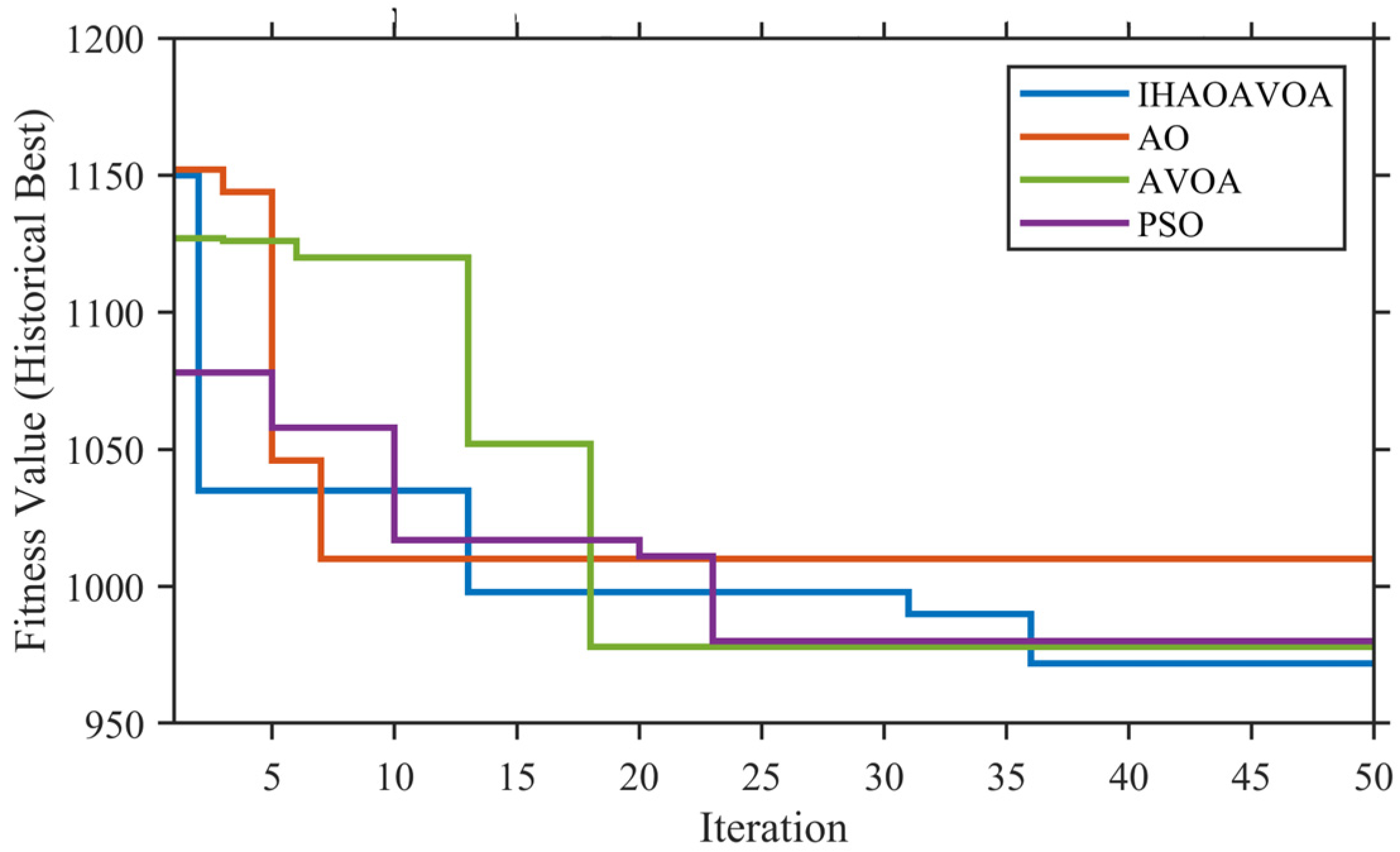
To evaluate the effectiveness of the proposed tuning strategy, the optimization results of the compared algorithms are analyzed in terms of both convergence behavior and final solution quality. The convergence curves are illustrated in Figure 2, while the corresponding quantitative results are summarized in

Table 2. Convergence characteristics and final fitness values of different optimization algorithms.

Algorithm	Early-Stage Best Fitness	Mid-Stage Best Fitness	Approximate Stabilization Iteration	Final Fitness
IHAOAVOA	1034.614215 (iter. 3)	998.234804 (iter. 13)	iter. 36	971.313291
AO	1045.138801 (iter. 6)	1010.754292 (iter. 8)	iter. 8	1010.754292
AVOA	1126.465286 (iter. 2)	1051.389579 (iter. 13)	iter. 18	977.901606
PSO	1057.965965 (iter. 5)	1017.080824 (iter. 10)	iter. 23	980.004862

.

As shown in Figure 2 and Table 2, the proposed IHAOAVOA achieves the best overall optimization performance among the compared methods. It exhibits a rapid reduction in the objective value in the early stage and maintains further improvement during the middle and late stages of the search process, finally obtaining the lowest fitness value. This result indicates that the proposed hybrid strategy provides a more effective balance between global exploration and local exploitation than the other compared algorithms.

By contrast, AO shows a relatively fast initial descent but tends to stagnate early, which suggests a limited late-stage refinement capability. AVOA and PSO both obtain competitive results, but their final fitness values remain higher than that of the proposed method. Overall, these results confirm that IHAOAVOA improves both convergence quality and final optimization performance for the controller parameter tuning problem through the adaptive combination of AO-based exploration and AVOA-based exploitation.

For completeness, the optimal four-dimensional controller parameter vectors obtained by the compared algorithms are listed in

Table 3. Optimal controller parameter vectors obtained using different optimization algorithms.

Algorithm	Optimal Parameter Vector
IHAOAVOA	$[0.0330336,0.262147,0.0064971,0.0364869]$
AO	$[0.151062,0.160980,0.0100000,0.1529260]$
AVOA	$[0.0412177,0.244252,0.0000273,0.0976135]$
PSO	$[0.0286550,0.152563,0.00804208,0.1258670]$

. The parameter order in each vector is $[\mathrm{c},\mathrm{q},\mathsf{\mu },{\mathrm{k}}_{\mathrm{e}}]$. The fractional order of the speed loop integrator is fixed as 0.8 and is therefore not included in the optimized parameter vector. Among the compared algorithms, IHAOAVOA obtains the lowest final fitness value, and its optimal parameter vector is

$$[\mathrm{c},\mathrm{q},\mathsf{\mu },{\mathrm{k}}_{\mathrm{e}}]=\left[\mathrm{0.0330336,0.262147,0.0064971,0.0364869}\right].$$

The results in Table 3 illustrate the optimization performance of the compared algorithms for the representative FOSMC tuning case. In the subsequent simulation study, the same tuning framework is applied to the corresponding operating conditions, and the final controller parameters used for each operating point are reported in Section 6.1.

After the stopping criterion is satisfied, the optimizer returns the best admissible parameter vector, which can be written as

$${\mathrm{x}}^{*}=\mathrm{a}\mathrm{r}\mathrm{g}\underset{\mathrm{x}}{\mathrm{m}\mathrm{i}\mathrm{n}}\mathrm{J}(\mathrm{x})$$

(46)

where ${\mathrm{x}}^{*}$ denotes the final optimized controller parameter vector. This vector represents the best solution under the predefined fitness function and feasibility constraints. In this way, the tuning process becomes automatic and reproducible, and the obtained controller parameters are directly aligned with the predefined control objective of achieving a fast response, reduced speed drop, low steady-state error, and suppressed speed ripple.

6. Simulation Results and Analysis

To verify the effectiveness of the proposed fractional-order sliding-mode control strategy and the IHAOAVOA-based tuning method, simulation studies were carried out on the PMSM-based flywheel energy storage system established in Simulink. The proposed method was evaluated from four aspects: speed loop dynamic response, performance consistency under different operating points, sensorless estimation accuracy, and electromagnetic torque behavior. For comparison, a conventional PI controller and a conventional integer-order sliding-mode controller (SMC) were also tested under the corresponding simulation conditions.

6.1. Simulation Setup

The simulations were performed on the PMSM–FESS model described in Section 3 under the idealized assumptions adopted in this work. The inverter and measurement channels were treated as ideal, while current, voltage, and speed constraints were imposed in the Simulink implementation to guarantee feasible operation. The controller parameters of the proposed FOSMC were obtained according to the tuning strategy introduced in Section 5, whereas the observer parameters were fixed according to the observer design requirements.

For numerical implementation, the fractional-order operators were implemented using the FOMCON-based Oustaloup recursive approximation rather than an explicit Grünwald–Letnikov finite-memory summation. The approximation frequency range was set to $[{10}^{-3},{10}^3]$ rad/s, and the approximation order was set to ${\mathrm{N}}_{\mathrm{o}}=5$. The speed loop fractional integrator used order 0.8, while the observer-related fractional integrator blocks used orders 1.98 and 0.98. The control sampling period was ${\mathrm{T}}_{\mathrm{s}}=1\times {10}^{-4}$ s, and the Simulink fixed-step size was $1\times {10}^{-6}$ s.

For the speed response comparison, two operating points were considered. At the 1000 rpm operating point, a 20 N·m load disturbance was applied at $\mathrm{t}=1.0$ s, and the total simulation duration was 2.0 s. At the 8000 rpm operating point, an 80 N·m load disturbance was applied at $\mathrm{t}=1.0$ s. The settling time and recovery time were evaluated using the ±2% error band, and the recovery time was measured from the disturbance instant $\mathrm{t}=1.0$ s.

For fair comparison, the PI, conventional SMC, and proposed FOSMC controllers were tuned under the same operating conditions and evaluated using the same fitness function in Equation (40). The final parameter sets are listed in

Table 4. Final controller parameters used under different operating conditions.

Operating Point	Controller	Parameters
1000 rpm	PI	${\mathrm{K}}_{\mathrm{p}}=4.8,{\mathrm{K}}_{\mathrm{i}}=0.016$
1000 rpm	SMC	$\mathrm{c}=4.5,{\mathrm{c}}_1=-0.5,\mathsf{\mu }=0.01,\mathrm{q}=3$
1000 rpm	FOSMC	$\mathrm{c}=0.014,\mathrm{q}=0.42,\mathsf{\mu }=0.0001,{\mathrm{k}}_{\mathrm{e}}=0.1$
8000 rpm	PI	${\mathrm{K}}_{\mathrm{p}}=0.3,{\mathrm{K}}_{\mathrm{i}}=0.002$
8000 rpm	SMC	$\mathrm{c}=6,{\mathrm{c}}_1=-0.7,\mathsf{\mu }=0.01,\mathrm{q}=1$
8000 rpm	FOSMC	$\mathrm{c}=0.01,\mathrm{q}=0.3,\mathsf{\mu }=0.0001,{\mathrm{k}}_{\mathrm{e}}=0.05$

. Since the 1000 rpm and 8000 rpm cases correspond to different speed levels and disturbance magnitudes, different controller parameter sets were adopted for the two operating points. For each operating point, all compared controllers were evaluated under the same disturbance setting, simulation duration, and performance indices. The final controller parameters used in the speed response comparisons are summarized in Table 4.

For the conventional SMC, $\mathrm{c}$ and ${\mathrm{c}}_1$ denote the sliding-surface coefficients, while $\mathsf{\mu }$ and $\mathrm{q}$ denote the switching gain and proportional reaching coefficient, respectively.

To examine the control performance under different operating conditions, the two representative operating points are used to evaluate the controller behavior under both moderate-speed and high-speed flywheel conditions. For quantitative evaluation, the rise time ${\mathrm{t}}_{\mathrm{r}}$ is defined as the time required for the response to increase from 10% to 90% of the reference value before the disturbance is applied. The settling time ${\mathrm{t}}_{\mathrm{s}}$ is defined as the first instant at which the response enters and remains within the ±2% error band before $\mathrm{t}=1.0$ s. The recovery time ${\mathrm{t}}_{\mathrm{r}\mathrm{e}\mathrm{c}}$ is defined as the time required for the response to re-enter and remain within the same ±2% band after the disturbance introduced at $\mathrm{t}=1.0$ s.

6.2. Speed Response Performance at Different Operating Points

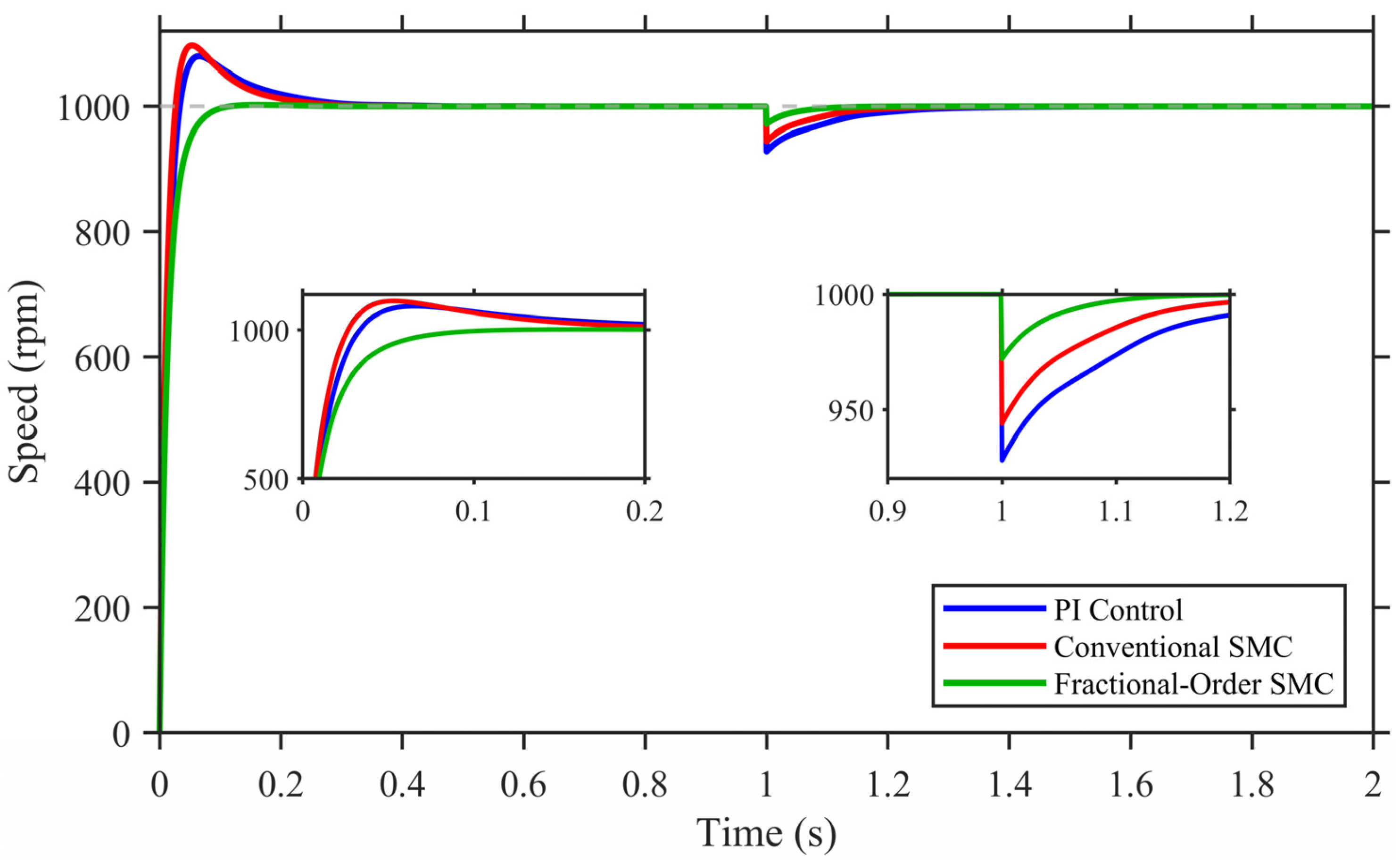
The speed responses of the three controllers at the 1000 rpm baseline under a 20 N·m load disturbance are shown in Figure 3. Under the same operating condition, the proposed FOSMC exhibits the smallest startup overshoot and the fastest post-disturbance recovery. As summarized in

Table 5. Quantitative speed response indices of the compared controllers.

Operating Point	Controller	Overshoot (%)	Speed Drop (%)	Settling Time (s)	Recovery Time (s)
1000 rpm	PI	8.0159	7.2000	0.1970	0.1230
1000 rpm	SMC	9.7416	5.6000	0.1670	0.0760
1000 rpm	FOSMC	0.2353	2.8000	0.0710	0.0130
8000 rpm	PI	1.5030	4.5000	0.0400	0.0620
8000 rpm	SMC	1.8266	3.6250	0.0310	0.0340
8000 rpm	FOSMC	0.0441	1.8750	0.0310	0.0000

, the startup overshoot is reduced to 0.2353%, whereas the PI control and conventional SMC show overshoots of 8.0159% and 9.7416%, respectively. After the disturbance is introduced at $\mathrm{t}=1.0$ s, the speed drop of the FOSMC is limited to 2.8000%, which is lower than 7.2000% for the PI control and 5.6000% for conventional SMC. These results indicate that the proposed controller improves both startup smoothness and low-speed disturbance rejection.

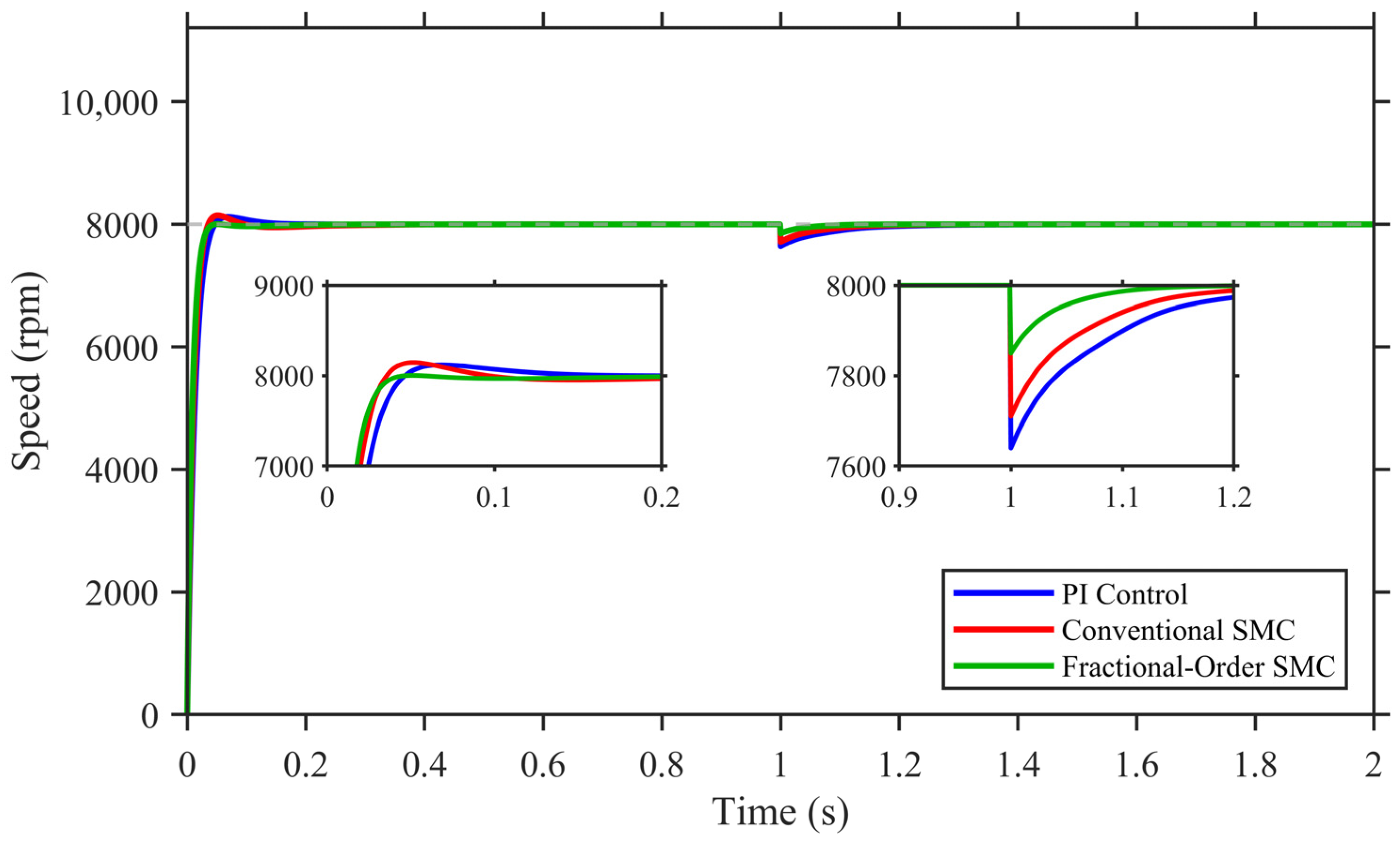
The speed responses at the 8000 rpm baseline under an 80 N·m load disturbance are presented in Figure 4. The proposed FOSMC still achieves the smallest overshoot and speed drop among the three compared controllers. Specifically, the overshoot is only 0.0441%, and the speed drop after the disturbance is 1.8750%. By contrast, the PI control and conventional SMC show larger speed deviations, as listed in Table 5. These results confirm that the proposed controller maintains robust speed regulation performance under the high-speed operating condition.

Taken together, the results at 1000 rpm and 8000 rpm demonstrate that the proposed FOSMC achieves a better balance among overshoot suppression, response rapidity, and disturbance recovery than the PI control and conventional SMC.

Since the speed deviation of the FOSMC at 8000 rpm remains within the predefined ±2% recovery band after the disturbance, its recovery time is recorded as 0 s according to the adopted definition.

6.3. Sensorless Speed Estimation Performance

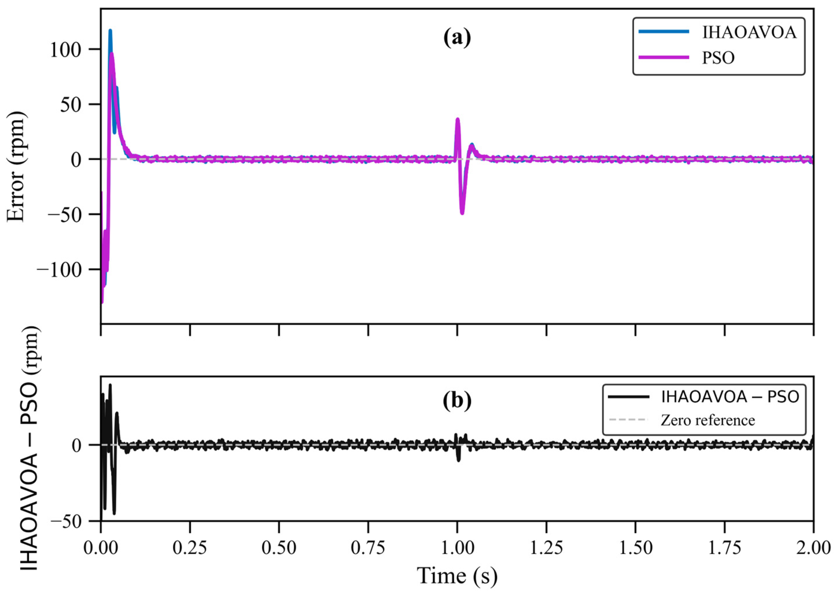
The speed estimation errors, defined as the difference between the estimated speed and the actual motor speed, at the 1000 rpm operating point are shown in Figure 5. The upper panel compares the estimation error curves, while the lower panel shows the difference between the IHAOAVOA-tuned and PSO-tuned cases. It can be observed that the IHAOAVOA-tuned scheme exhibits a smaller startup estimation error and improved transient convergence behavior than its PSO-tuned counterpart. In particular, the maximum startup error is reduced from about 40.9 r/min to about 34.5 r/min, and the response enters the ±5 r/min band earlier. After the disturbance is introduced at t = 1.0 s, both methods remain stable, while the proposed method still shows a slightly smaller post-disturbance peak estimation error, which is limited to about 48.0 r/min, compared with about 52.2 r/min for the PSO-tuned case. This indicates that the proposed tuning strategy mainly improves the startup estimation transient at the 1000 rpm operating point, while also providing a modest advantage in post-disturbance estimation performance.

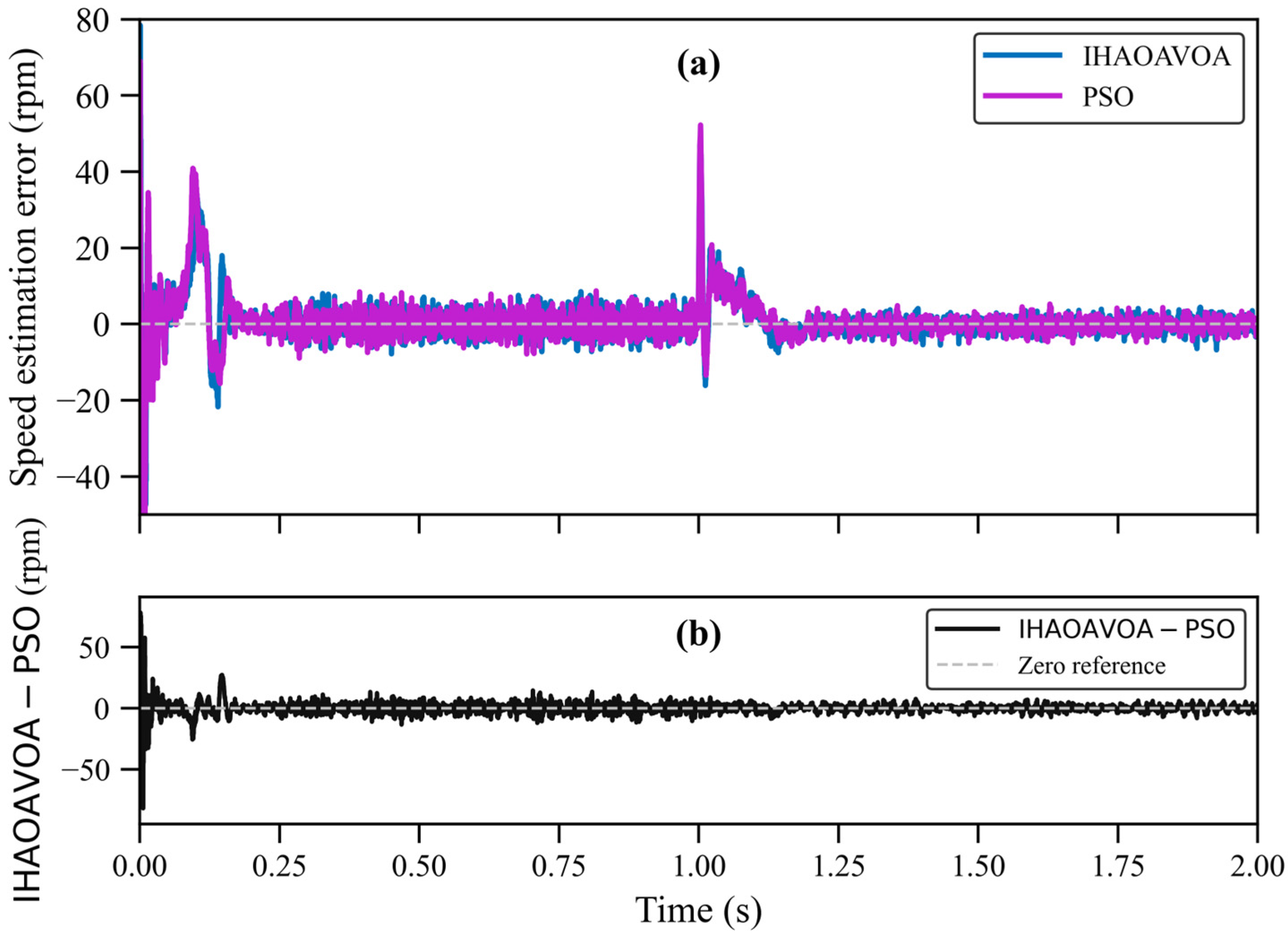
The corresponding speed estimation errors at the 8000 rpm operating point are shown in Figure 6. The upper panel compares the estimation error curves, while the lower panel gives the difference curve between IHAOAVOA and PSO. Although both methods exhibit a comparable initial estimation transient, the IHAOAVOA-tuned scheme enters the ±10 r/min band earlier, at 0.0671 s, compared with 0.0718 s for PSO. The post-disturbance peak error is also slightly reduced from 49.2632 r/min to 48.1579 r/min. Therefore, the proposed tuning strategy mainly improves transient convergence and post-disturbance estimation behavior under the high-speed operating condition.

Overall, the results at both operating points demonstrate that the IHAOAVOA-tuned controller improves the transient quality of sensorless speed estimation. This improvement is mainly reflected in the startup transient at the 1000 rpm operating point and in the convergence speed and post-disturbance estimation behavior at the 8000 rpm operating point. These results indicate that the IHAOAVOA-based tuning strategy improves not only the speed loop regulation performance but also the dynamic quality of observer-based sensorless operation.

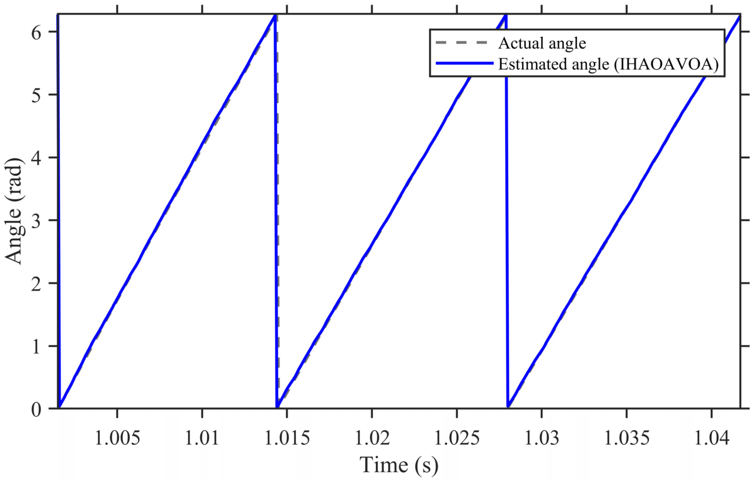
6.4. Rotor Angle Estimation Performance

Figure 7 shows the rotor angle estimation performance of the proposed method at the 1000 rpm operating point. In the displayed interval, the estimated angle closely follows the actual angle. Their variation trends, slopes, and periodic reset positions are highly consistent, which indicates that the observer can maintain accurate phase tracking under sensorless operation. Only a slight local estimation deviation can be observed, while the overall error remains small. In the displayed interval, the maximum angle error is about 0.067 rad and the RMSE is about 0.029 rad, corresponding to approximately 0.011 p.u. and 0.005 p.u., respectively, when normalized by 2π. Therefore, the proposed sensorless scheme under the IHAOAVOA-tuned controller is able to provide stable and accurate rotor-angle estimation.

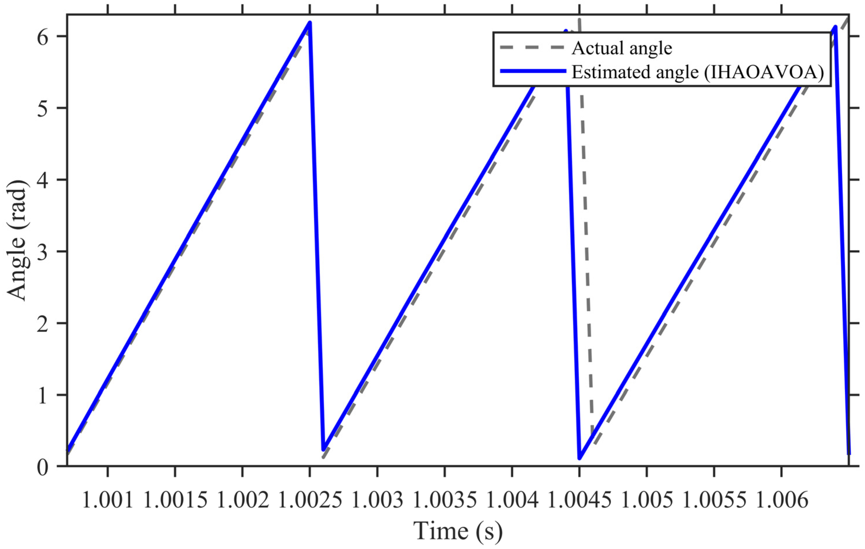
The corresponding rotor-angle estimation results at the 8000 rpm baseline are presented in Figure 8. Under the high-speed operating condition, the estimated angle remains generally consistent with the actual angle over the displayed interval. Although a visible local deviation can be observed around the periodic reset positions, the two curves still maintain similar variation trends and slopes. This indicates that the proposed sensorless scheme can preserve the rotor-angle tracking capability under the 8000 rpm operating condition. From the displayed interval, the estimation deviation remains bounded, and the overall angle-tracking behavior can be regarded as stable.

Taken together, the results at both operating points demonstrate that the proposed sensorless scheme can provide accurate and stable rotor-angle information for closed-loop operation over a wide speed range. The results also indicate that the proposed control framework supports reliable sensorless PMSM-driven FESS operation under different operating conditions.

6.5. Electromagnetic Torque Characteristics

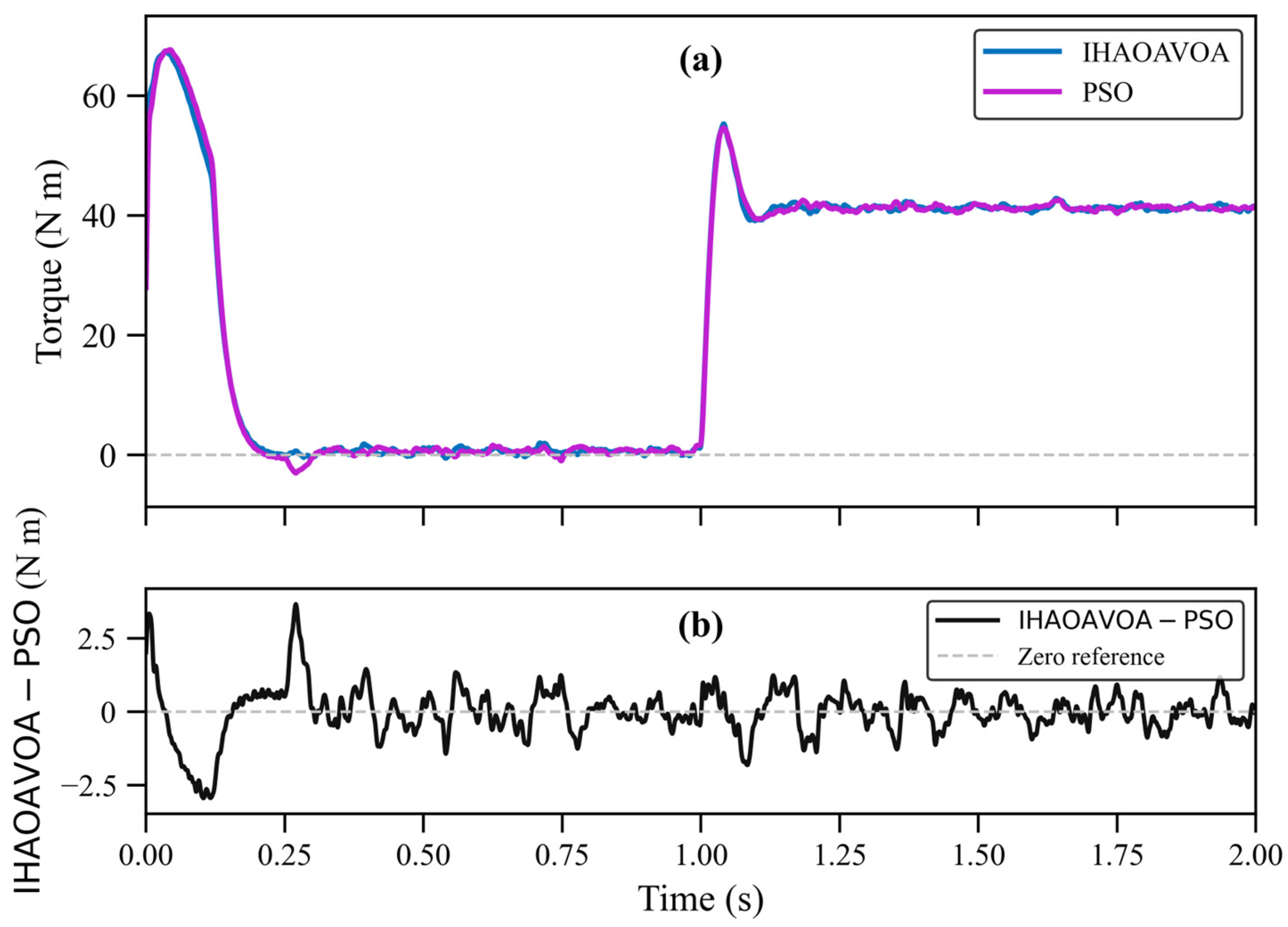
Figure 9 shows the electromagnetic torque responses at the 1000 rpm operating point, together with the corresponding torque difference curve. The two tuning methods exhibit similar steady-state torque behavior, while the added difference curve makes the transient deviation more visible. Compared with PSO, IHAOAVOA slightly reduces the startup torque peak and more clearly suppresses the negative torque undershoot. Therefore, the advantage of IHAOAVOA in this case is mainly reflected in improved transient torque smoothness, while only a modest improvement can be observed in steady-state torque ripple.

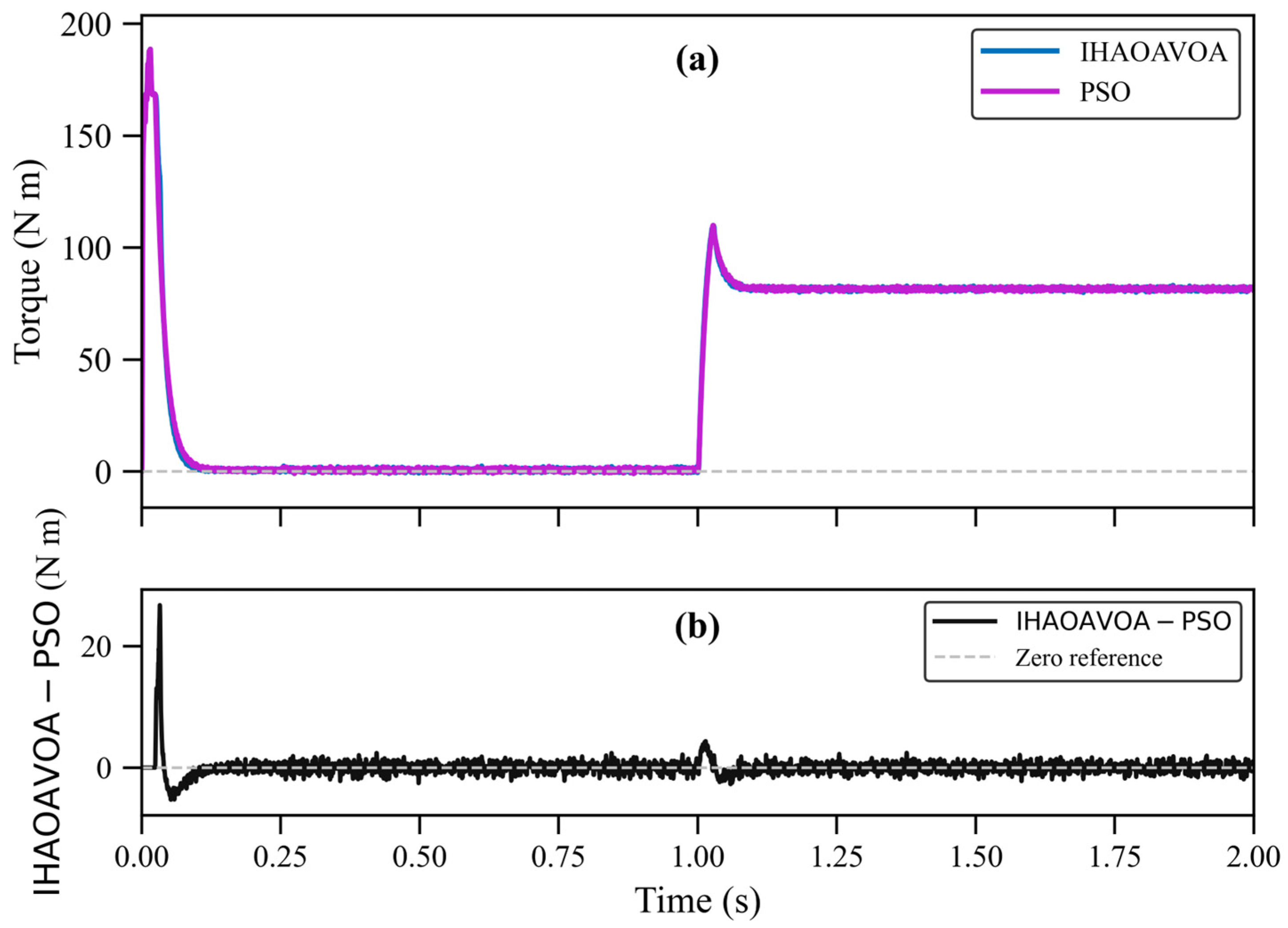
The corresponding electromagnetic torque responses at the 8000 rpm operating point are shown in Figure 10. The torque curves of IHAOAVOA and PSO are nearly overlapped in the steady-state intervals, indicating comparable steady-state torque regulation. The difference curve shows that the main deviation appears during the startup transient, whereas only a small, short-duration deviation can be observed after the disturbance, and the steady-state difference remains very limited. This result indicates that the proposed tuning strategy maintains stable torque behavior under high-speed operation, with its advantage mainly reflected in transient torque regulation.

Overall, the results at both operating points demonstrate that the IHAOAVOA-based tuning strategy mainly improves the transient quality of electromagnetic torque regulation while maintaining comparable steady-state torque behavior. This improvement is beneficial for enhancing the smoothness and robustness of PMSM-driven FESS operation over a wide speed range.

6.6. Discussion

The above results demonstrate that the proposed control framework improves both the speed regulation and sensorless estimation performance of the PMSM-driven FESS. In terms of speed regulation, the FOSMC provides smaller startup overshoot and speed drop than the PI control and conventional integer-order SMC under both 1000 rpm and 8000 rpm operating conditions, while maintaining comparable or faster settling and recovery behavior. In particular, under the 20 N·m disturbance at the 1000 rpm operating point, the proposed controller limits the speed drop to 2.8000%, whereas the PI control and conventional SMC show larger drops of 7.2000% and 5.6000%, respectively. Under the 80 N·m disturbance at the 8000 rpm operating point, the proposed controller also achieves the smallest speed drop among the compared controllers.

For sensorless estimation, the sensorless control scheme with the IHAOAVOA-tuned the FOSMC improves the transient convergence behavior compared with PSO tuning. At the 8000 rpm operating point, although both methods exhibit the same maximum startup estimation error, IHAOAVOA enters the ±10 r/min band earlier and slightly reduces the post-disturbance peak error. This indicates that the proposed tuning strategy is beneficial for improving the dynamic quality of observer-based speed estimation.

The electromagnetic torque results further show that IHAOAVOA and PSO produce very close steady-state torque behavior. The benefit of IHAOAVOA is mainly observed in the transient intervals, especially in reducing the negative torque undershoot at the 1000 rpm operating point and maintaining comparable torque smoothness under both operating points. Therefore, the proposed method improves the overall transient quality of the PMSM-driven FESS without degrading steady-state torque regulation.

7. Conclusions

This paper proposed a sensorless control framework for PMSM-based flywheel energy storage systems by combining the FOSMC, the FOSMO, and IHAOAVOA-based parameter tuning. The fractional-order operators were implemented using the FOMCON-based Oustaloup recursive approximation, and the controller parameters were optimized using a five-term objective function considering ITAE, overshoot, post-disturbance speed dip, steady-state error, and speed ripple.

The simulation results show that the proposed FOSMC achieves better speed loop performance than a PI control and a conventional integer-order SMC. At the 1000 rpm operating point under a 20 N·m load disturbance, the proposed method reduces the startup overshoot to 0.2353% and limits the post-disturbance speed drop to 2.8000%. At the 8000 rpm operating point under an 80 N·m disturbance, the proposed method also provides the smallest overshoot and speed drop among the compared controllers.

In sensorless operation, the IHAOAVOA-tuned scheme improves the transient convergence of speed estimation compared with PSO tuning. The torque results further show that IHAOAVOA and PSO have comparable steady-state torque behavior, while IHAOAVOA improves transient torque smoothness, especially by reducing the negative torque undershoot at the 1000 rpm operating point. Overall, the proposed framework provides an effective balance among fast speed regulation, disturbance rejection, sensorless estimation accuracy, and electromechanical transient smoothness.

8. Future Work

Although the proposed sensorless FOSMC–FOSMO framework has been verified through simulation, further work is still required before practical engineering application. Future research will focus on hardware experimental validation and on extending the proposed method to more complex operating scenarios, including parameter drift, inverter nonidealities, loss effects, thermal effects, and broader charge–discharge cycling conditions. In addition, the implementation burden of the fractional-order operators and the real-time feasibility of the proposed control scheme will be further evaluated on an experimental platform.

References

- Faraji, F.; Majazi, A.; Al-Haddad, K. A comprehensive review of flywheel energy storage system technology. Renew. Sustain. Energy Rev. 2017, 67, 477–490. [Google Scholar] [CrossRef]
- Arani, A.A.K.; Gharehpetian, G.B.; Abedi, M. Review of flywheel energy storage systems structures and applications in power systems and microgrids. Renew. Sustain. Energy Rev. 2017, 69, 9–18. [Google Scholar] [CrossRef]
- Li, X.; Palazzolo, A. A review of flywheel energy storage systems: State of the art and opportunities. J. Energy Storage 2022, 46, 103576. [Google Scholar] [CrossRef]
- Amiryar, M.E.; Pullen, K.R. A review of flywheel energy storage system technologies and their applications. Appl. Sci. 2017, 7, 286. [Google Scholar] [CrossRef]
- Sebastián, R.; Peña Alzola, R. Flywheel energy storage systems: Review and simulation for an isolated wind power system. Renew. Sustain. Energy Rev. 2012, 16, 6803–6813. [Google Scholar] [CrossRef]
- Zhang, J.W.; Wang, Y.H.; Liu, G.C.; Tian, G.Z. A review of control strategies for flywheel energy storage system and a case study with matrix converter. Energy Rep. 2022, 8, 3948–3963. [Google Scholar] [CrossRef]
- Karrari, S.; Carne, M.; Buticchi, G.; Liserre, M.; Wheeler, P. Model validation of a high-speed flywheel energy storage system using power hardware-in-the-loop testing. J. Energy Storage 2021, 43, 103177. [Google Scholar] [CrossRef]
- Pillay, P.; Krishnan, R. Application characteristics of permanent magnet synchronous and brushless DC motors for servo drives. IEEE Trans. Ind. Appl. 1991, 27, 986–996. [Google Scholar] [CrossRef]
- Jiang, X.; Liu, X.; Jiang, J.; Xu, Y. Design and analysis of a highly reliable permanent magnet synchronous machine for flywheel energy-storage systems. Machines 2024, 12, 655. [Google Scholar] [CrossRef]
- Xiang, B.; Wang, X.; Wong, W.O. Process control of charging and discharging of magnetically suspended flywheel energy storage system. J. Energy Storage 2022, 47, 103629. [Google Scholar] [CrossRef]
- Wu, L.G.; Liu, J.; Vazquez, S.; Mazumder, S.K. Sliding mode control in power converters and drives: A review. IEEE/CAA J. Autom. Sin. 2022, 9, 392–406. [Google Scholar] [CrossRef]
- Urbanski, K. Sensorless control of the permanent magnet synchronous motor with selected state estimators. Sensors 2019, 19, 3546. [Google Scholar] [CrossRef] [PubMed]
- Olabi, O.A.; Wilberforce, T.; Abdelkareem, M.A.; Ramadan, M. Critical review of flywheel energy storage system. Energies 2021, 14, 2159. [Google Scholar] [CrossRef]
- Xu, K.; Shen, Y.; Chen, J.; Wang, Y.; Liu, J. A review of flywheel energy storage system technologies. Energies 2023, 16, 6462. [Google Scholar] [CrossRef]
- Choudhury, S. Flywheel energy storage systems: A critical review on technologies, applications, and future prospects. Int. Trans. Electr. Energy Syst. 2021, 31, e13024. [Google Scholar] [CrossRef]
- Jia, Y.; Wu, Z.; Zhang, J.; Yang, P.; Zhang, Z. Control strategy of flywheel energy storage system based on primary frequency modulation of wind power. Energies 2022, 15, 1850. [Google Scholar] [CrossRef]
- Díaz-González, F.; Sumper, A.; Gomis-Bellmunt, O.; Villafáfila-Robles, R. A review of energy storage technologies for wind power applications. Renew. Sustain. Energy Rev. 2012, 16, 2154–2171. [Google Scholar] [CrossRef]
- Li, T.; Sun, X.D.; Lei, G.; Yang, Z.B.; Guo, Y.G.; Zhu, J.G. Finite-control-set model predictive control of permanent-magnet synchronous motor drive systems—An overview. IEEE/CAA J. Autom. Sin. 2022, 9, 2087–2105. [Google Scholar] [CrossRef]
- Peng, J.; Yao, M. Overview of predictive control technology for permanent magnet synchronous motor systems. Appl. Sci. 2023, 13, 6255. [Google Scholar] [CrossRef]
- Preindl, M.; Bolognani, S. Model predictive direct speed control with finite control set of PMSM drive systems. IEEE Trans. Power Electron. 2013, 28, 1007–1015. [Google Scholar] [CrossRef]
- Liu, Y.; Meng, K.; Liang, K.; Wang, H.; Zhang, Y. Research on control strategy of flywheel energy storage system based on active disturbance rejection control. AIP Adv. 2023, 13, 115332. [Google Scholar] [CrossRef]
- Qu, L.; Qiao, W.; Qu, L. An extended-state-observer-based sliding-mode speed control for permanent-magnet synchronous motors. IEEE J. Emerg. Sel. Top. Power Electron. 2021, 9, 1605–1613. [Google Scholar] [CrossRef]
- Wang, A.; Jia, X.; Dong, S. A new exponential reaching law of sliding mode control to improve performance of permanent magnet synchronous motor. IEEE Trans. Magn. 2013, 49, 2409–2412. [Google Scholar] [CrossRef]
- Zhang, X.; Sun, L.; Zhao, K.; Sun, L. Nonlinear speed control for PMSM system using sliding-mode control and disturbance compensation techniques. IEEE Trans. Power Electron. 2013, 28, 1358–1365. [Google Scholar] [CrossRef]
- Xu, W.; Jiang, Y.; Mu, C.; Blaabjerg, F. Novel composite sliding mode control for PMSM drive system based on disturbance observer. IEEE Trans. Appl. Supercond. 2016, 26, 0605005. [Google Scholar] [CrossRef]
- Zaihidee, F.M.; Mekhilef, S.; Mubin, M. Fractional order PID sliding mode control for speed regulation of permanent magnet synchronous motor. J. Eng. Res. 2021, 9, 209–218. [Google Scholar] [CrossRef]
- Kim, H.; Son, J.-B.; Lee, J. A high-speed sliding-mode observer for the sensorless speed control of a PMSM. IEEE Trans. Ind. Electron. 2011, 58, 4069–4077. [Google Scholar]
- Zhang, Y.; Cheng, X.-F. Sensorless control of permanent magnet synchronous motors and EKF parameter tuning research. Math. Probl. Eng. 2016, 2016, 3916231. [Google Scholar] [CrossRef]
- Zuo, Y.; Lai, C.; Iyer, K.L.V. A review of sliding mode observer based sensorless control methods for PMSM drive. IEEE Trans. Power Electron. 2023, 38, 11352–11374. [Google Scholar] [CrossRef]
- Pillay, P.; Krishnan, R. Modeling, simulation, and analysis of permanent-magnet motor drives. I. The permanent-magnet synchronous motor drive. IEEE Trans. Ind. Appl. 1989, 25, 265–273. [Google Scholar] [CrossRef]
- Hu, H.; Xu, Z.; Yu, X.; Zhang, Y. Multirate model predictive current control of a permanent magnet synchronous motor for flywheel energy storage systems. Energy Rep. 2022, 8, 11490–11501. [Google Scholar]
- Xiang, B.; Wu, S.; Wen, T.; Liu, H.; Peng, C. Design, modeling, and validation of a 0.5 kWh flywheel energy storage system using magnetic levitation system. Energy 2024, 308, 132867. [Google Scholar] [CrossRef]