Bifurcation Analysis and Chaotic Behaviors of and a Traveling-Wave Solution to the Zhiber–Shabat Equation with a Truncated M-Fractional Derivative

Abstract

In this article, we use truncated M-fractional derivatives to analyze the bifurcation and chaotic behavior of and traveling-wave solutions to the Zhiber–Shabat equation. By introducing truncated M-fractional derivatives, the equation exhibits richer dynamic properties. Based on phase diagram analysis and dynamical system theory, the bifurcation behavior of the equilibrium point of a two-dimensional dynamical system is discussed. At the same time, the dynamical behavior of a two-dimensional dynamical system with periodic disturbances is considered, revealing the complex chaotic phenomena of the system under specific parameters. A planar phase diagram, a three-dimensional phase diagram, a sensitivity analysis, and a maximum Lyapunov exponent diagram of the perturbed two-dimensional dynamical system were employed. Furthermore, various forms of accurate analytical solutions were obtained through traveling-wave transformation and numerical simulation. The three-dimensional, two-dimensional, density, and polar coordinates of the solutions were plotted using mathematical software. The results indicate that the fractional order and system parameters have a significant impact on the morphology and chaotic characteristics of the solution. This study provides new theoretical insights into the nonlinear dynamics of fractional-order Zhiber–Shabat equations.

1. Introduction

In the field of nonlinear science, exploring and obtaining exact solutions to nonlinear partial differential equations (NLPDEs) [1,2,3,4,5] play a crucial role in understanding complex nonlinear phenomena in various disciplines such as physics, fluid mechanics, plasma physics, biology, and nonlinear optics. The solitary waves [6], periodic waves [7], rogue waves [8], bifurcation behavior [9], and chaotic behavior [10,11] in these NLPDEs profoundly reveal the intrinsic structures and evolutionary laws of nonlinear systems. In recent years, many scholars have focused their research on investigating analytical solutions to and analyzing the dynamic behaviors of these complex nonlinear systems. Several important research methods, such as dynamical system analysis, the auxiliary function method, and the polynomial complete discriminant system method, have been proposed for studying analytical solutions and dynamic behaviors in nonlinear system [12]. The nonlinear Zhiber–Shabat equation [13,14,15], a model with a significant physical background, has been an active research direction in nonlinear science. Analysis of its exact solutions and dynamic behaviors provides a theoretical foundation for further understanding the interactions and influences in nonlinear wave propagation processes.

In recent years, with the rapid development of mathematical theories, mathematical–physical models with memory and non-local characteristics have often been simulated using fractional nonlinear partial differential equations (FNLPDEs) [16,17,18,19]. Unlike integer-order derivatives, there are many types of fractional derivatives, such as truncated M-fractional derivatives [20], conformable fractional derivatives [21], and beta fractional derivatives [22]. The M-derivative has garnered significant attention due to its satisfaction of the chain rule and its well-defined operational properties. Particularly, its truncated form plays an important role in computational efficiency and physical applicability. Based on these considerations, the study of NLPDEs with M-derivatives is of great importance. In such fractional-order models, the dynamic behavior of the nonlinear Zhiber–Shabat (ZS) equation with a truncated M-fractional derivative, as well as the chaotic behavior of perturbed systems, still requires systematic investigation.

In summary, the aim of this study is to apply the truncated M-fractional derivative to the ZS equation and conduct a comprehensive dynamic analysis of the resulting model. The specific research objectives are given below:

(1)

We used the bifurcation theory of a dynamical system to analyze the equilibrium points and create bifurcation parameter diagrams;

(2)

We studied the chaotic behavior of a system under specific parameters and excitations and identified and characterized chaotic motion through numerical methods such as phase portraits, sensitivity analysis, and Lyapunov exponent;

(3)

Based on the results of a bifurcation analysis, we used the homogeneous equilibrium method to solve the equation, obtaining and classifying various types of analytical solutions in the sense of truncated M-fractional derivatives, such as soliton solutions, periodic solutions, and kink solutions.

This study is expected not only to deepen our understanding of the complex dynamics of the fractional ZS equation but also to provide new ideas and methodological references for solving and analyzing related nonlinear fractional-order models. The ZS equation with a truncated M-fractional derivative is described as follows [23]:

$$D_{M,xt}^{2\alpha ,\beta }u+p{e}^u+q{e}^{-u}+r{e}^{-2u}=0,$$

(1)

where $u=u(x,t)$ is an unknown function. The parameters p, q, and r are real constants. This equation is widely used in the fields of fluid dynamics, integral quantum field theory, and nonlinear optics. When $\alpha =1$, Equation (1) is transformed into the nonlinear ZS equation, which is an integer-order version of the PDE. When $r=0$, Equation (1) is transformed into the well-known Sinh–Gordon equation [24]. Moreover, when $q=r=0$, Equation (1) is further simplified into the Liouville equation. Similarly, when $q=0$, Equation (1) is transformed into the Dodd–Bullough–Mikhailov equation [25]. When $p=0$, $q=-1$, and $r=1$, Equation (1) is simplified to the Tzitzeica–Dodd–Bullough equation [26]. In this article, we will use traveling-wave solutions and dynamic behavior analysis of the ZS equation under a truncated M-fractional order, with the main objective being to explore the dynamic behavior of the ZS equation in the context of fluid mechanics, integral quantum field theory, and nonlinear optics. Compared with existing approaches in the literature (see [24,25,26]), the equation considered in this paper is a more general ZS equation. The ZS equation considered in this paper is a fractional-order ZS equation, and the dynamic behavior of Equation (1) is also considered. The traveling-wave solutions to Equation (1) are also provided, including more general Jacobian function solutions. The definition of a truncated M-fractional derivative is described as follows.

Definition 1

([27,28]). [Truncated M-fractional derivative] For a function $g:[0,\infty )\to (-\infty ,+\infty )$, the truncated M-fractional derivative of g of the order α is defined by

$$D_M^{\alpha ,\beta }g\left(t\right)=\underset{\epsilon \to 0}{lim}{\displaystyle \frac{g\left(t{E}_{\beta }\left(\epsilon t^{1-\alpha }\right)\right)-g\left(t\right)}{\epsilon }}, 0<\alpha \le 1, \beta >0, \forall t>0,$$

(2)

where $E_{\beta }(·)$ represents the one-parameter-truncated Mittag–Leffler function.The properties of the truncated M-fractional derivative can be referred to in reference [27,28].

The subsequent sections are arranged as follows: In Section 2, the analytical solutions to the nonlinear Zhiber–Shabat equation with a truncated M-fractional derivative are constructed based on the tank homogeneous equilibrium method. In Section 3, a qualitative analysis of a two-dimensional dynamical system under periodic disturbances is presented, and a phase diagram, sensitivity analysis diagram, and maximum Lyapunov exponent diagram of the system are provided. In Section 4, 3D, 2D, density, and polar plots of some solutions to Equation (1) are plotted with given parameters. In Section 5, a brief conclusion is given. In Section 6, future research is provided.

2. Analytical Solutions to Equation (1)

In order to further investigate the exact solution to Equation (1), we first present the following traveling-wave transformation:

$$u(x,t)=\psi \left(\xi \right), \xi ={\displaystyle \frac{\Gamma (\beta +1)}{\epsilon }}(x^{\alpha }-c{t}^{\alpha }),$$

(3)

where c is a nonzero constant representing the wave speed.

Substituting transformation (3) into Equation (1) yields the following nonlinear ordinary differential equation:

$$-c{\psi }^{″}+p{e}^{\psi }+q{e}^{-\psi }+r{e}^{-2\psi }=0.$$

(4)

In order to construct the solution to Equation (4), we make the following assumptions:

$$v=e^{\psi } or \psi =\ln v.$$

(5)

By plugging Equation (5) into Equation (4), we have

$$c[{\left(v^{\prime }\right)}^2-v{v}^{″}]+p{v}^3+qv+r=0.$$

(6)

Based on the rank homogeneous polynomial method [29], we employ the probing equation:

$$v^{″}=a_2{v}^2+a_{1}v+a_0.$$

(7)

Integrating Equation (7) once yields

$${\left(v^{\prime }\right)}^2={\displaystyle \frac{2}{3}}{a}_2{v}^3+a_1{v}^2+2a_{0}v+d,$$

(8)

where $a_2$, $a_1$, $a_0$, and d are all nonzero constants.

Substituting Equations (7) and (8) into Equation (6) yields a polynomial concerning v, with coefficients of zero, resulting in an algebraic system of equations. Solving this algebraic system of equations yields

$$a_2=-{\displaystyle \frac{3p}{c}}, a_1=a_1, a_0=-{\displaystyle \frac{q}{c}}, d=-{\displaystyle \frac{r}{c}}.$$

In order to develop all solutions to Equation (8), we first make the following assumptions:

$$w={\left({\displaystyle \frac{2a_2}{3}}\right)}^{{\displaystyle \frac{1}{3}}}v, d_2=a_1{\left({\displaystyle \frac{2a_2}{3}}\right)}^{-{\displaystyle \frac{2}{3}}}, d_1=a_0{\left({\displaystyle \frac{2a_2}{3}}\right)}^{-{\displaystyle \frac{1}{3}}}, d_0=d.$$

Based on the above assumptions, Equation (8) can be rewritten as

$${\left(w^{\prime }\right)}^2=w^3+d_2{w}^2+d_{1}w+d_0,$$

(9)

and its expression is

$$\pm {\left(a_3\right)}^{{\displaystyle \frac{1}{3}}}(\xi -{\xi }_0)=\int {\displaystyle \frac{1}{\sqrt{w^3+d_2{w}^2+d_{1}w+d_0}}}d\xi .$$

(10)

Here, we make the assumption that $f\left(w\right)=w^3+d_2{w}^2+d_{1}w+d_0$. Its complete discrimination system is

$$\left\{\begin{array}{c}\mathsf{{\rm Y}}=-27{({\displaystyle \frac{2d_2^2}{27}}+d_0-{\displaystyle \frac{d_1{d}_2}{3}})}^2-4{(d_1-{\displaystyle \frac{d_2^2}{3}})}^3,\hfill \\ D_1=d_1-{\displaystyle \frac{d_2^2}{3}}.\hfill \end{array}\right.$$

(11)

By using to Liu’s complete discriminant system method [30], we can obtain the traveling-wave solution to Equation (1).

Case 1: $\mathsf{{\rm Y}}=0$, $D_1<0$

In this case, $f\left(w\right)=0$ has a triple real root and a double real root, which means that $f\left(w\right)={(w-a)}^2(w-b)$, where $a\ne b$. Therefore, when $w>a$, Equation (10) can be rewritten as

$$\pm (\xi -{\xi }_0)=\int {\displaystyle \frac{dw}{(w-a)\sqrt{w-b}}}=\left\{\begin{array}{c}{\displaystyle \frac{1}{\sqrt{a-b}}}\ln \left|{\displaystyle \frac{\sqrt{w-b}-\sqrt{a-b}}{\sqrt{w-b}+\sqrt{a-b}}}\right|, a>b,\hfill \\ {\displaystyle \frac{2}{\sqrt{b-a}}}\arctan \sqrt{{\displaystyle \frac{w-b}{b-a}}}, a<b.\hfill \end{array}\right.$$

(12)

Next, we can integrate Equation (15) to obtain the solutions to Equation (1):

$$\begin{array}{c}\hfill {\psi }_1(t,x)=\ln [{({\displaystyle \frac{2}{3}}{a}_2)}^{-{\displaystyle \frac{1}{3}}}(b+(a-b){\tanh }^2({\displaystyle \frac{\sqrt{a-b}}{2}}{({\displaystyle \frac{2}{3}}{a}_2)}^{{\displaystyle \frac{1}{3}}}({\displaystyle \frac{\Gamma (\beta +1)}{\epsilon }}(x^{\alpha }-c{t}^{\alpha })-{\xi }_0)))], a>b.\end{array}$$

$$\begin{array}{c}\hfill {\psi }_2(t,x)=\ln [{({\displaystyle \frac{2}{3}}{a}_2)}^{-{\displaystyle \frac{1}{3}}}(b+(a-b){\coth }^2({\displaystyle \frac{\sqrt{a-b}}{2}}{({\displaystyle \frac{2}{3}}{a}_2)}^{{\displaystyle \frac{1}{3}}}({\displaystyle \frac{\Gamma (\beta +1)}{\epsilon }}(x^{\alpha }-c{t}^{\alpha })-{\xi }_0)))], a>b.\end{array}$$

$$\begin{array}{c}\hfill {\psi }_3(t,x)=\ln [{({\displaystyle \frac{2}{3}}{a}_2)}^{-{\displaystyle \frac{1}{3}}}(b+(b-a){\tan }^2({\displaystyle \frac{\sqrt{b-a}}{2}}{({\displaystyle \frac{2}{3}}{a}_2)}^{{\displaystyle \frac{1}{3}}}({\displaystyle \frac{\Gamma (\beta +1)}{\epsilon }}(x^{\alpha }-c{t}^{\alpha })-{\xi }_0)))], a<b.\end{array}$$

Case 2: $\mathsf{{\rm Y}}=0$, $D_1=0$

In this case, $f\left(w\right)=0$ has a triple root, which means that $f\left(w\right)={(w-c)}^3$. Thus, Equation (10) can be rewritten as

$$\begin{array}{c}\hfill {\psi }_4(t,x)=\ln [4{({\displaystyle \frac{2}{3}}{a}_2)}^{-{\displaystyle \frac{2}{3}}}{\displaystyle \frac{1}{{(\frac{\Gamma (\beta +1)}{\epsilon }(x^{\alpha }-c{t}^{\alpha })-{\xi }_0)}^2}}+c].\end{array}$$

Case 3: $\mathsf{{\rm Y}}>0$, $D_1<0$

In this case, $f\left(w\right)=0$ has three different real roots, $l_1$, $l_2$, and $l_3$, and satisfies $l_1<l_2<l_3$, which means that $f\left(w\right)=(w-l_1)(w-l_2)(w-l_3)$. When $l_1<w<l_3$, we employ a transformation: $w=l_1+(l_2-l_1){\sin }^2\zeta$. Thus, Equation (10) can be rewritten as

$$\begin{array}{cc}\hfill \pm (\xi -{\xi }_0)& =\int {\displaystyle \frac{dw}{\sqrt{(w-l_1)(w-l_2)(w-l_3)}}}=\int {\displaystyle \frac{2(l_2-l_1)\sin \zeta \cos \zeta d\zeta }{\sqrt{l_3-l_1}(l_2-l_1)\sin \zeta \cos \zeta \sqrt{1-m^2{\sin }^2\zeta }}}\hfill \\ \hfill & ={\displaystyle \frac{2}{\sqrt{l_3-l_1}}}\int {\displaystyle \frac{d\zeta }{\sqrt{1-m^2{\sin }^2\zeta }}},\hfill \end{array}$$

(13)

where $m^2={\displaystyle \frac{l_2-l_1}{l_3-l_1}}$.

From the above equation and the definition of an Jacobian elliptic sine function, it can be seen that $w=l_1+(l_2-l_1){\mathbf{sn}}^2({\displaystyle \frac{\sqrt{l_3-l_1}}{2}}{\displaystyle \frac{\sqrt{l_3-l_1}}{2}}(\xi -{\xi }_0),m)$. Therefore, the solution to Equation (1) is

$$\begin{array}{c}\hfill {\psi }_5(t,x)=\ln [{({\displaystyle \frac{2}{3}}{a}_2)}^{-{\displaystyle \frac{1}{3}}}(l_1+(l_2-l_1){\mathbf{sn}}^2({\displaystyle \frac{\sqrt{l_3-l_1}{(\frac{2}{3}{a}_2)}^{\frac{1}{3}}}{2}}({\displaystyle \frac{\Gamma (\beta +1)}{\epsilon }}(x^{\alpha }-c{t}^{\alpha })-{\xi }_0),m))].\end{array}$$

When $w>l_3$, we realize the following transformation: $w={\displaystyle \frac{-l_2{\sin }^2\zeta +l_3}{{\cos }^2\zeta }}$. Similarly, we can obtain the solution to Equation (1):

$$\begin{array}{c}\hfill {\psi }_6(t,x)=\ln [{({\displaystyle \frac{2}{3}}{a}_2)}^{-{\displaystyle \frac{1}{3}}}{\displaystyle \frac{l_3-l_2{\mathbf{sn}}^2(\frac{\sqrt{l_3-l_1}}{2}{(\frac{2}{3}{a}_2)}^{\frac{1}{3}}(\frac{\Gamma (\beta +1)}{\epsilon }(x^{\alpha }-c{t}^{\alpha })-{\xi }_0),m)}{{\mathbf{cn}}^2(\frac{\sqrt{l_3-l_1}}{2}{(\frac{2}{3}{a}_2)}^{\frac{1}{3}}(\frac{\Gamma (\beta +1)}{\epsilon }(x^{\alpha }-c{t}^{\alpha })-{\xi }_0),m)}}].\end{array}$$

Case 4:  $\mathsf{{\rm Y}}<0$

In this case, $f\left(w\right)=0$ has only one real root, which means that $f\left(w\right)=(w-s)(w^2+s_{2}w+s_1)$, where $s_2^2-4s_1<0$. When $w>s$, we employ a transformation: $w=s+\sqrt{s^2+s_{2}s+s_1}{\tan }^2{\displaystyle \frac{\eta }{2}}$. Thus, Equation (10) can be rewritten as

$$\begin{array}{cc}\hfill \pm (\xi -{\xi }_0)& =\int {\displaystyle \frac{dw}{\sqrt{(w-s)(w^2+s_{2}w+s_1)}}}=\int {\displaystyle \frac{\sqrt{s^2+s_{2}s+s_1\frac{\tan \frac{\eta }{2}}{{\cos }^2\frac{\eta }{2}}}}{{(s^2+s_{2}s+s_1)}^{\frac{3}{4}}\frac{\tan \frac{\eta }{2}}{{\cos }^2\frac{\eta }{2}}\sqrt{1-n^2{\sin }^2\eta }}}\hfill \\ \hfill & ={\displaystyle \frac{1}{{(s^2+s_{2}s+s_1)}^{\frac{1}{4}}}}\int {\displaystyle \frac{d\eta }{\sqrt{1-n^2{\sin }^2\eta }}},\hfill \end{array}$$

(14)

where $n^2={\displaystyle \frac{1}{2}}(1-{\displaystyle \frac{s+\frac{s_2}{2}}{\sqrt{s^2+s_{2}s+s_1}}})$.

From the above equation and the definition of an elliptic cosine function, it can be seen that $\mathbf{cn}({(s^2+s_{2}s+s_1)}^{{\displaystyle \frac{1}{4}}}(\xi -{\xi }_0),n)=\cos \eta$. So, we can find that

$$\cos \eta ={\displaystyle \frac{2\sqrt{s^2+s_{2}s+s_1}}{w-s+\sqrt{s^2+s_{2}s+s_1}}}-1.$$

(15)

Therefore, when $w>s$, the solution to Equation (1) is

$$\begin{array}{cc}\hfill {\psi }_7(t,x)& =\ln [{({\displaystyle \frac{2}{3}}{a}_2)}^{-{\displaystyle \frac{1}{3}}}(s+{\displaystyle \frac{2\sqrt{s^2+s_{2}s+s_1}}{1+\mathbf{cn}({(s^2+s_{2}s+s_1)}^{\frac{1}{4}}{(\frac{2}{3}{a}_2)}^{-\frac{1}{3}}(\frac{\Gamma (\beta +1)}{\epsilon }(x^{\alpha }-c{t}^{\alpha })-{\xi }_0),n)}}\hfill \\ \hfill & -\sqrt{s^2+s_{2}s+s_1})].\hfill \end{array}$$

3. Qualitative Analysis

Assuming ${\displaystyle \frac{dv}{d\xi }}=z$, the two-dimensional dynamical system of Equation (7) can be rewritten as

$$\left\{\begin{array}{c}{\displaystyle \frac{dv}{d\xi }}=z,\hfill \\ {\displaystyle \frac{dz}{d\xi }}=a_2{v}^2+a_{1}v+a_0,\hfill \end{array}\right.$$

(16)

and its first integral is

$$H(z,v)={\displaystyle \frac{1}{2}}{z}^2-{\displaystyle \frac{1}{3}}{a}_2{v}^3-{\displaystyle \frac{1}{2}}{a}_1{v}^2-a_{0}v=h,$$

(17)

where h is an integral constant.

Suppose that $g\left(v\right)=a_2{v}^2+a_{1}v+a_0$, $g^{\prime }\left(v\right)=2a_2+a_1$ and $\Delta =a_1^2-4a_0{a}_2$. Thus, if $\Delta >0$, there are two different roots for $g\left(v\right)=0$, denoted as $v_1={\displaystyle \frac{-a_1+\sqrt{\Delta }}{2a_2}}$ and $v_2={\displaystyle \frac{-a_1-\sqrt{\Delta }}{2a_2}}$. If $\Delta =0$, $g\left(v\right)=0$ has only one root, denoted as $v_3=-{\displaystyle \frac{a_1}{2a_2}}$. Thus, the classification of equilibrium points and their phase portraits in Equation (16) are given.

Case 1: When $\Delta >0$, the equilibrium point $(v_1,0)$ is a saddle point.

Case 2: When $\Delta <0$, the equilibrium point $(v_2,0)$ is a center point.

Case 3: When $a_1<0$ and $\Delta =0$, the equilibrium point $(v_3,0)$ is a saddle point. When $a_1>0$ and $\Delta =0$, the equilibrium point $(v_3,0)$ is a center point.

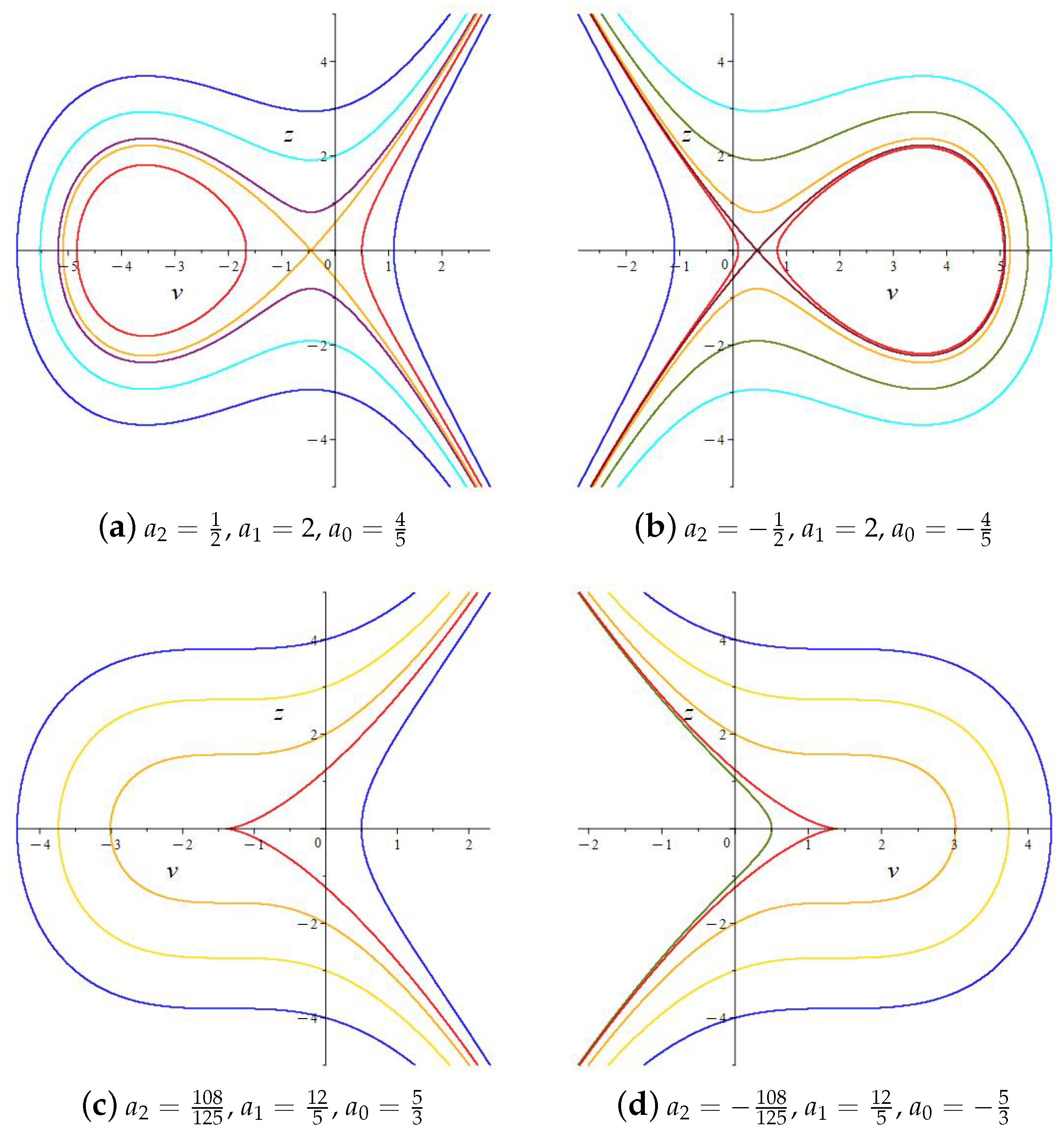
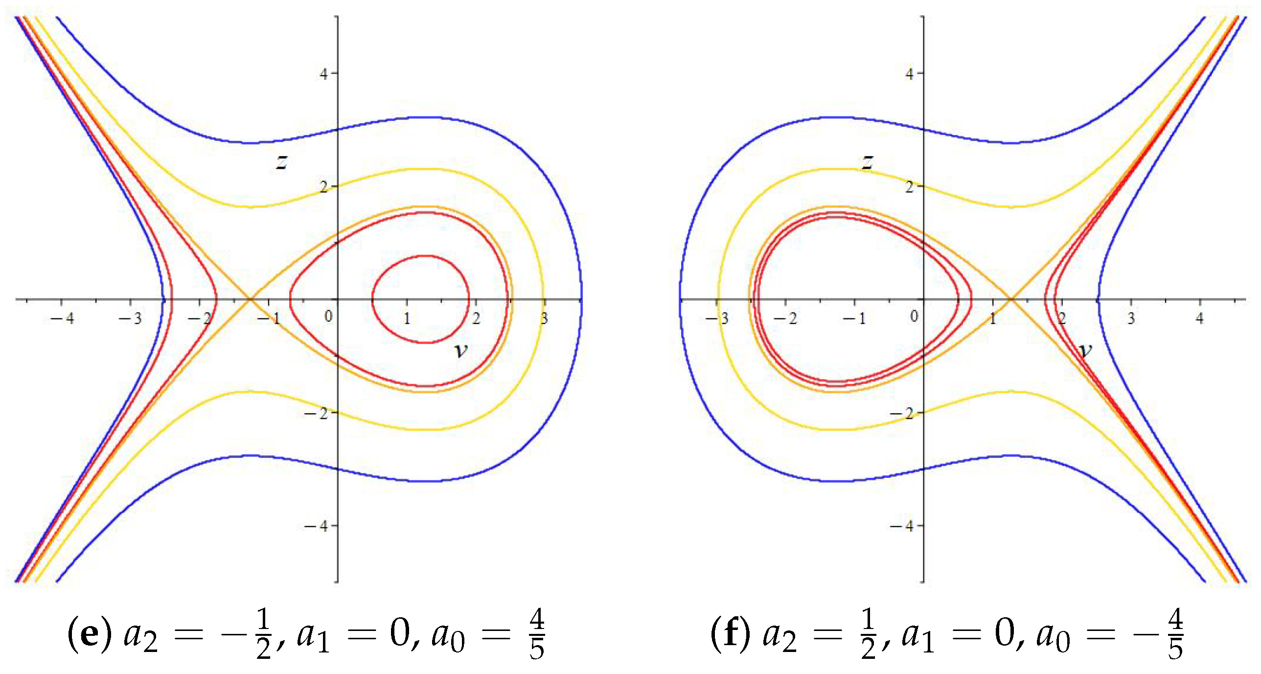
Based on the above classification, we used Maple mathematical software to create a phase portrait, as shown in Figure 1. It is worth noting that by analyzing the types of equilibrium points such as saddle points and centers, the stability of the solution to system (7) can be determined. The orbit in Figure 1 and the solution to Equation (1) have corresponding topological properties. The orbit of the same orbit corresponds to the soliton solution to Equation (16). The heteroclinic orbit corresponds to the twisted and anti-twisted solutions to Equation (16). The periodic wave solution for the closed orbit of Equation (1) is also given.

Next, we consider the dynamic behavior of a two-dimensional system with periodic disturbances:

$$\left\{\begin{array}{c}{\displaystyle \frac{dv}{d\xi }}=z,\hfill \\ {\displaystyle \frac{dz}{d\xi }}=a_2{v}^2+a_{1}v+a_0+A\cos \left(k\xi \right)+B\sin \left(l\xi \right),\hfill \end{array}\right.$$

(18)

where A, B, k, and l are the real constant.

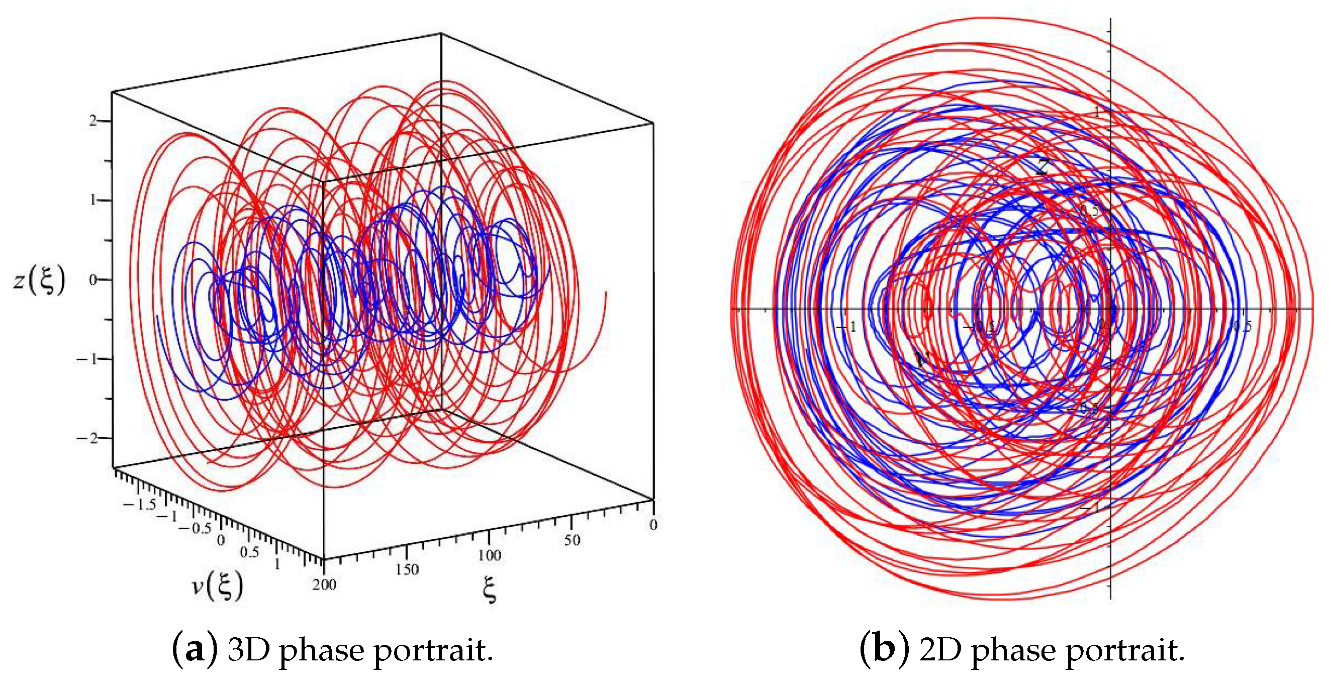
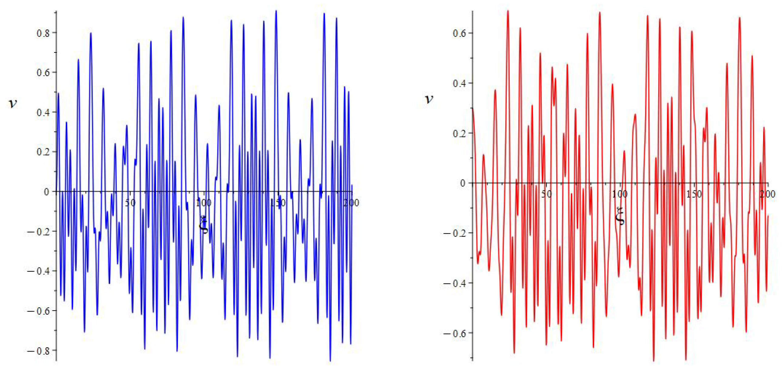
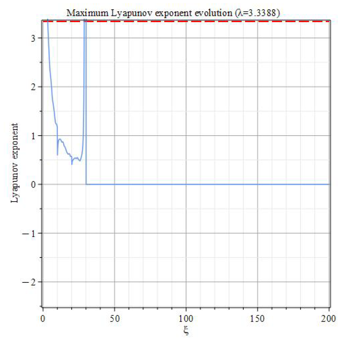
In this stage, we used Maple mathematical software to create two-dimensional and three-dimensional phase portraits of Equation (18) and conducted a sensitivity analysis of Equation (18) under different initial values, as shown in Figure 2 and Figure 3. And we also plotted the maximum Lyapunov exponent graph, as shown in Figure 4. By combining Figure 2, Figure 3 and Figure 4, we can draw a conclusion. That is, when the maximum Lyapunov exponent is greater than zero, it indicates the existence of chaos in the system. In Figure 2 and Figure 3, there is a slight difference in the initial values of the system, while the orbital properties of the system undergo significant changes.

4. Numerical Simulation

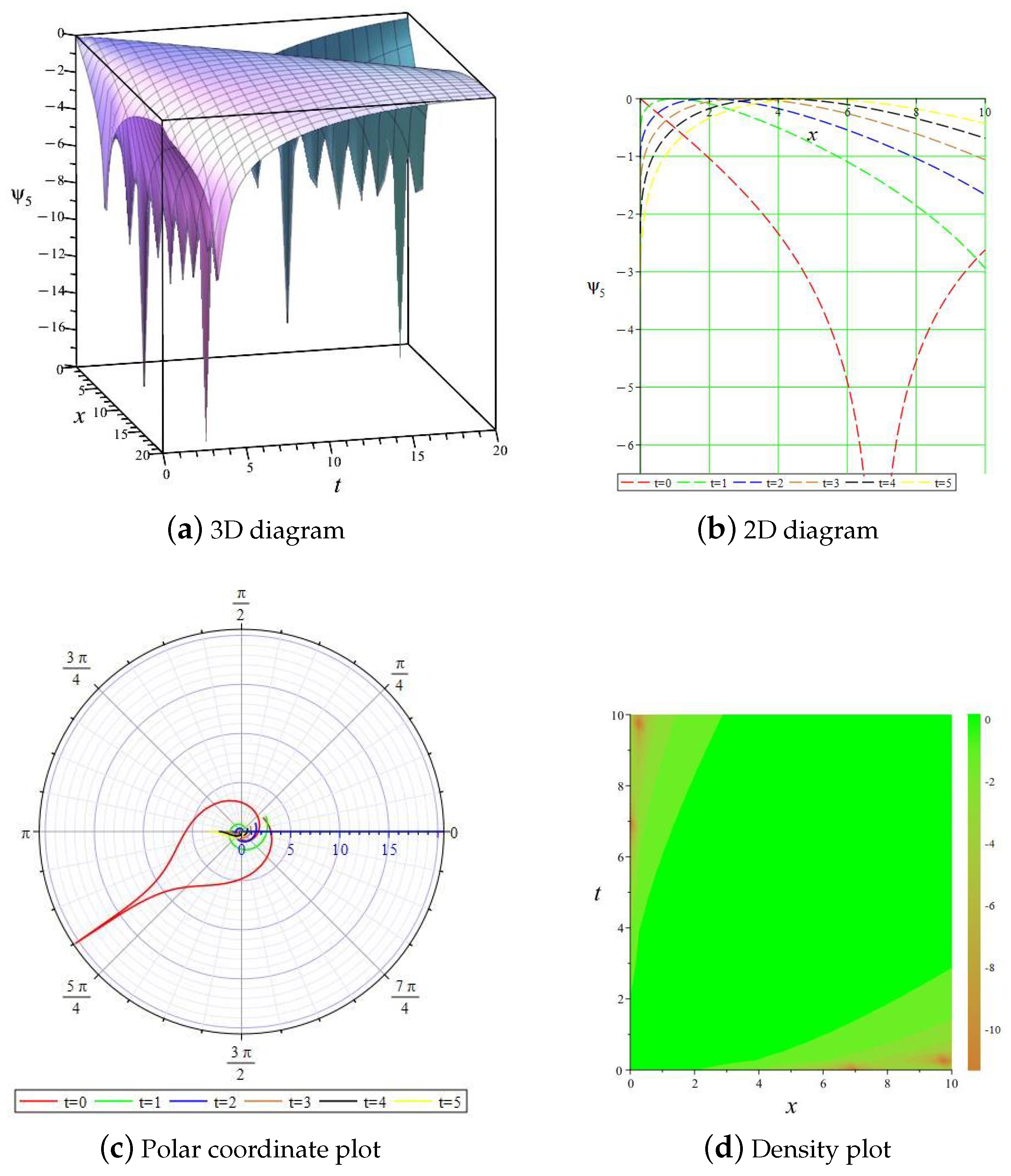
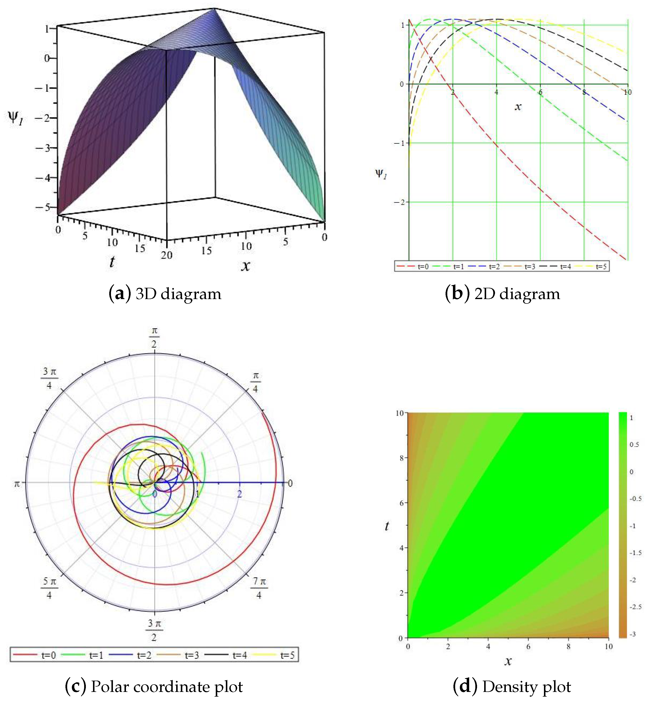
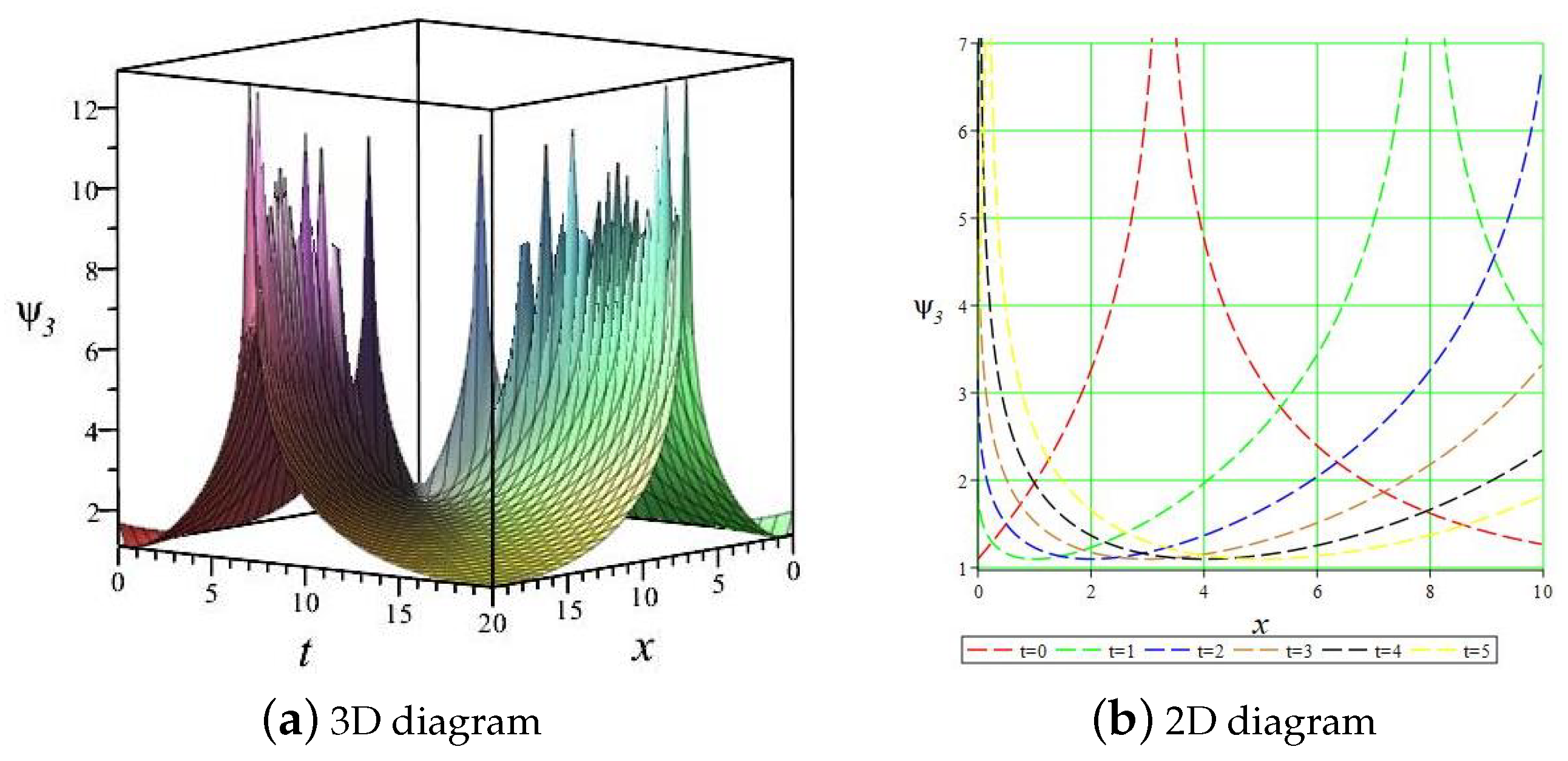
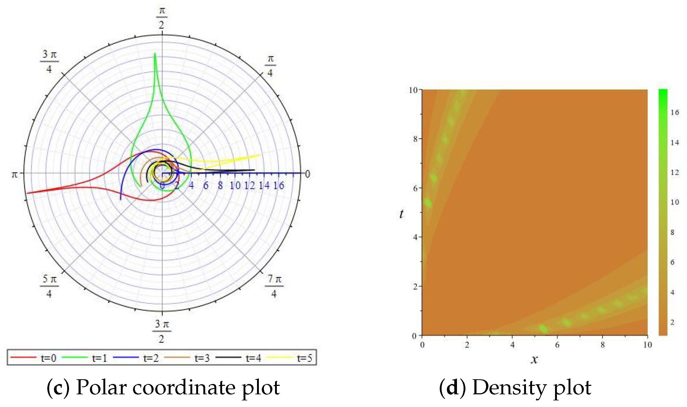
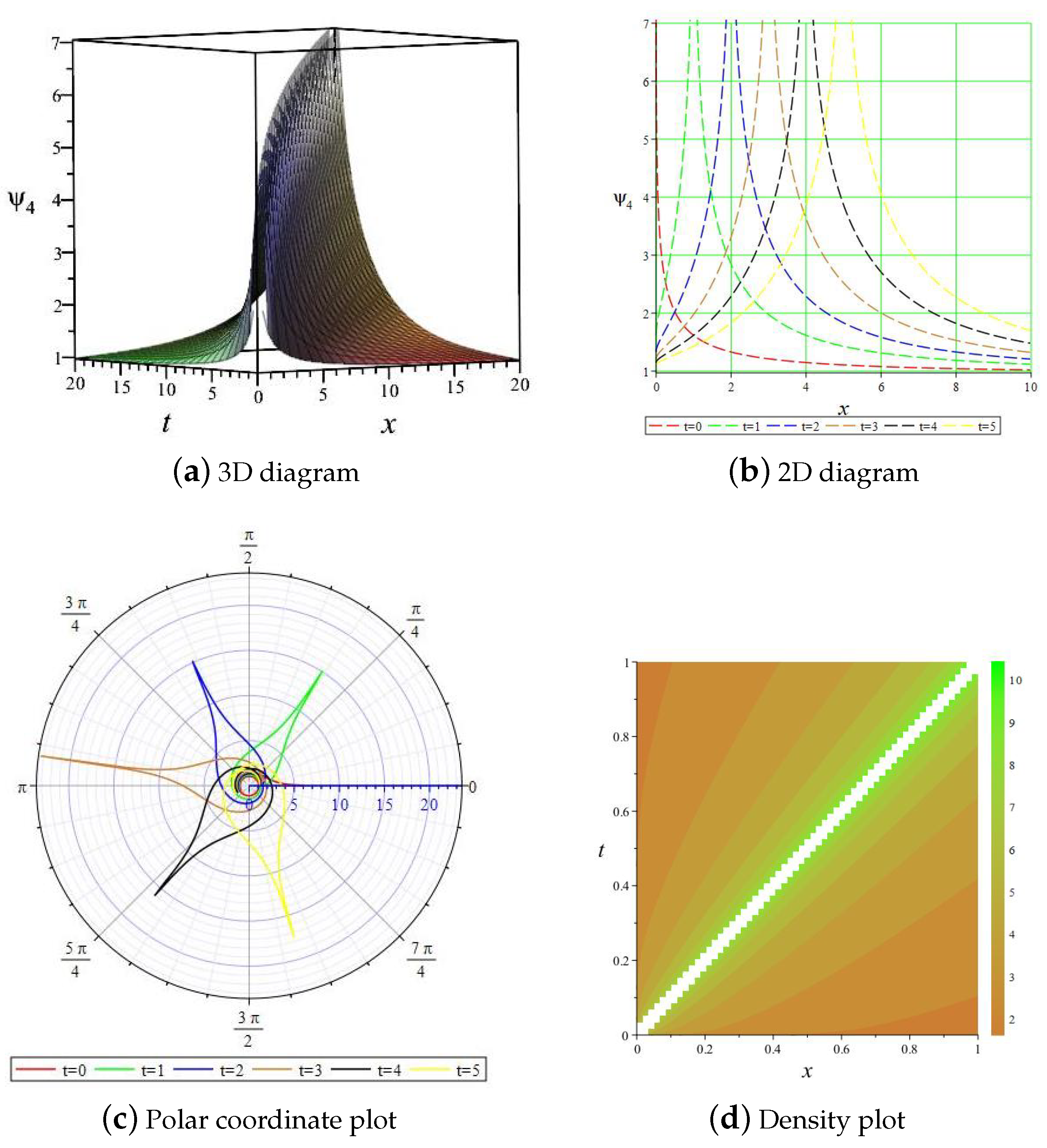
Next, we selected specific parameters to create three-dimensional, two-dimensional, contour map, and polar coordinate images for the analytical solution to Equation (1) in order to visually demonstrate the solution structure under different functional forms. When the parameters are set to $\alpha ={\displaystyle \frac{1}{2}}$, $\beta =1$, $\epsilon =1$, $a_2={\displaystyle \frac{3}{2}}$, $a_1=3$, $a_0=0$, $d=0$, and ${\xi }_0=0$, the explicit solution ${\psi }_1(t,x)$ appears in the form of a bell-shaped solitary wave, as shown in Figure 5. When the parameters are set to $\alpha ={\displaystyle \frac{1}{2}}$, $\beta =1$, $\epsilon =1$, $a_2={\displaystyle \frac{3}{2}}$, $a_1=-3$, $a_0=0$, $d=0$, and ${\xi }_0=0$, the explicit solution ${\psi }_3(t,x)$ appears in the form of a periodic solution, as shown in Figure 6. When the parameters are set to $\alpha ={\displaystyle \frac{1}{2}}$, $\beta =1$, $\epsilon =1$, $a_2={\displaystyle \frac{3}{2}}$, $a_1=3$, $a_0=3$, $d=1$, and ${\xi }_0=0$, the explicit solution ${\psi }_3(t,x)$ appears in the form of a trigonometric function solution, as shown in Figure 7. When the parameters are set to $\alpha ={\displaystyle \frac{1}{2}}$, $\beta =1$, $\epsilon =1$, $a_2={\displaystyle \frac{3}{2}}$, $a_1=0$, $a_0=-1$, $d=0$, $m={\displaystyle \frac{\sqrt{2}}{2}}$, and ${\xi }_0=0$, the explicit solution ${\psi }_5(t,x)$ appears in the form of a periodic function solution, as shown in Figure 8.

Remark 1.

The three-dimensional diagram in Figure 5a presents the global shape of the solution in $x-t-\psi$ space; the two-dimensional cross-sectional view in Figure 5b depicts the evolution of the spatiotemporal contour over time; the polar coordinate diagram in Figure 5c reveals the possible periodic/rotational behavior in the spatiotemporal plane as per our understanding; and the density plot in Figure 5d highlights the amplitude distribution throughout the entire spatiotemporal domain. By jointly analyzing these graphs, we can gain a deeper understanding of the dynamic behavior, spatiotemporal dependencies, and main qualitative characteristics of the solution to Equation (1) under specific parameters. Figure 6, Figure 7 and Figure 8 also have similar characteristics. The explicit solution ${\psi }_3(t,x)$ is a singular solution that typically describes physical quantities that tend towards infinity at isolated points or curves (such as shock wave fronts, optical vortices, dislocation nuclei, and the “eyewall” structure of atmospheric vortices).

5. Conclusions

This paper investigated the dynamic and chaotic behavior of and traveling-wave solutions to the ZS equation with truncated M-fractional derivatives. The results show that the introduction of fractional derivatives significantly enriches the dynamic behavior of the system’s solutions. Theoretical analysis revealed that the introduction of fractional derivatives and changes in key system parameters can effectively regulate the stability of the equilibrium point. Under periodic disturbances, the system exhibited clear chaotic behavior within a specific parameter range, which was effectively verified through plotting Lyapunov exponent diagrams. At the same time, we obtained the traveling-wave solutions in various forms of equations, including solitary waves and periodic waves, whose waveforms, amplitudes, and propagation velocities have been shown to strongly depend on fractional derivatives. This study not only expands our theoretical understanding of the dynamics of the classical ZS equation in the fractional-order framework but also reveals the synergistic control mechanism of parameters with respect to bifurcation paths, chaos generation, sensitivity analysis, and traveling-wave solution forms. It also provides new analytical ideas and theoretical foundations for the application of related fractional-order nonlinear models in the fields of physics and engineering.

6. Future Research

Based on the research in this article, future research work can focus on the following directions: (1) extending fractional operators to other fractional-order operators (such as conformal and beta derivatives) and comparing their dynamic characteristics; (2) studying high-dimensional or coupled ZS systems and exploring more complex wave structures such as rogue waves and breathers; and (3) considering more realistic disturbances, such as random noise and time-delay feedback, and developing direct numerical methods for the original fractional partial differential equations.

References

1. Beenish; Samreen, M. Exploring symmetry and bifurcation structures in nonlinear electrical lattices with soliton solutions. Phys. Lett. A 2026, 578, 131440. [Google Scholar] [CrossRef]
2. Hussain, E.; Shah, S.A.A.; Muhammad Naveed Rafiq, M.N.R.; Ragab, A.E.; Az-Zo’bi, E. Exact solutions and modulation instability analysis of a generalized Kundu-Eckhaus equation with extra-dispersion in optical fibers. Phys. Scr. 2024, 99, 055222. [Google Scholar] [CrossRef]
3. Iqbal, I.; Boulaaras, S.M.B.; Saad Althobaiti, S.; Althobaiti, A.; Rehman, H. Exploring soliton dynamics in the nonlinear Helmholtz equation: Bifurcation, chaotic behavior, multistability, and sensitivity analysis. Nonlinear Dyn. 2025, 113, 16933–16954. [Google Scholar] [CrossRef]
4. Mahmood, S.S.; Murad, M.A.S. Optical solutions of weakly nonlocal media for nonlinear conformable Schrödinger equation by extended simplest equation method. Phys. Lett. A 2025, 560, 130936. [Google Scholar] [CrossRef]
5. Tang, L. Bifurcation analysis, chaotic behavior, cubic-quartic optical solitons and phase portraits for the nonlinear coupled Kaup-Newell equation in birefringent fibers. Math. Methods Appl. Sci. 2026, 49, 239–253. [Google Scholar] [CrossRef]
6. Flamarion, M.V.; Pelinovsky, E. Emergence of champion solitons from two-solitary-wave interactions in the fourth-order generalized Korteweg–de Vries equation. Chaos Soliton Fractals 2026, 208, 118271. [Google Scholar] [CrossRef]
7. Dai, Y.F.; An, T.R.; Wei, M.Z.; Zhang, H.Y. Periodic and solitary waves in a generalized delayed KP-MEW equation with arbitrarily high-order nonlinearity. Commun. Nonlinear Sci. Numer. Simul. 2026, 159, 109876. [Google Scholar] [CrossRef]
8. Qiu, T.W.; Wang, M.E.; Wang, Z.; Liu, K.X.; Sun, J.M. Modulational instability, rogue waves and multi-pole solitons for the fifth-order reverse space-time nonlinear Schrödinger equation. Phys. D Nonlinear Phenom. 2026, 488, 135101. [Google Scholar] [CrossRef]
9. Wang, J.; Li, Z. The impact of standard Wiener process on the qualitative analysis and traveling wave solutions of stochastic nonlinear Kodama equation in the Stratonovich sense. AIMS Math. 2025, 10, 24997–25010. [Google Scholar] [CrossRef]
10. Hussain, A.; Chaudhary, U.A.; Junaid-U-Rehman, M.; Jhangeer, A. Stability, sensitivity, chaotic behavior, and soliton solution of the perturbed Kaup-Newell equation. Ain Shams Eng. J. 2026, 17, 104097. [Google Scholar] [CrossRef]
11. Tang, L. Qualitative analysis, traveling wave solutions and chaotic behavior for the perturbed Schrödinger-Hirota equation with cubic-quintic-septic law of self-phase modulation. Mod. Phys. Lett. B 2025, 40, 2550170. [Google Scholar] [CrossRef]
12. Tang, C.; Li, X.Q.; Wang, Q. Solvability of indefinite stochastic LQ optimal control problems for jump diffusion models. J. Dyn.Control Syst. 2026, 32, 9. [Google Scholar] [CrossRef]
13. He, B.; Long, Y.; Rui, W.G. New exact bounded travelling wave solutions for the Zhiber–Shabat equation. Nonlinear Anal. Theory Methods Appl. 2009, 71, 1636–1648. [Google Scholar] [CrossRef]
14. Wazwaz, A.M. The tanh method for travelling wave solutions to the Zhiber–Shabat equation and other related equations. Commun. Nonlinear Sci. Numer. Simul. 2008, 13, 584–592. [Google Scholar] [CrossRef]
15. Inc, M. New type soliton solutions for the Zhiber–Shabat and related equations. Optik 2017, 138, 1–7. [Google Scholar] [CrossRef]
16. Li, Z. Bifurcation and traveling wave solution to fractional Biswas-Arshed equation with the beta time derivative. Chaos Solitons Fractals 2022, 160, 112249. [Google Scholar]
17. Santra, S.; Behera, R. Simultaneous space–time Hermite wavelet method for time-fractional nonlinear weakly singular integro-partial differential equations. Commun. Nonlinear Sci. Numer. Simul. 2025, 140, 108324. [Google Scholar] [CrossRef]
18. Li, H.R.; Zhao, W.; Zhang, X.H. Stability and convergence analysis of reduced-order finite difference schemes for a class of nonlinear time-fractional partial differential equations. J. Math. Anal. Appl. 2026, 559, 130465. [Google Scholar] [CrossRef]
19. Zayed, E.M.E.; Amer, Y.A.; Shohib, R.M.A. The fractional complex transformation for nonlinear fractional partial differential equations in the mathematical physics. J. Assoc. Arab. Univ. Basic Appl. Sci. 2016, 19, 59–69. [Google Scholar] [CrossRef]
20. Bibi, M.; Saleem, M.S.; Rehman, H.U. Soliton dynamics of the Landau–Ginzburg–Higgs and generalized Kadomtsev–Petviashvili modified equal width Burgers equations for the truncated M-fractional derivative. Z. Naturforsch. A 2025, 80, 0125. [Google Scholar] [CrossRef]
21. Li, Z. Solving the exactly explicit solutions of the conformable space-time fractional Phi-4 equation via neural networks method. Phys. Lett. A 2026, 581, 131535. [Google Scholar] [CrossRef]
22. Li, Z.; Peng, C. Bifurcation, phase portrait and traveling wave solution of time-fractional thin-film ferroelectric material equation with beta fractional derivative. Phys. Lett. A 2023, 484, 129080. [Google Scholar] [CrossRef]
23. Muhammad, J.; Younas, U. Dynamics of new truncated M-fractional derivative wave structures to the nonlinear Zhiber-Shabat equation arising in variety of fields. Int. J. Math. Comput. Eng. 2026, 4, 145–160. [Google Scholar]
24. Bernatska, J. Exact quasi-periodic solutions to the sine(sinh)-Gordon equations: The method for computation and analysis. Phys. D Nonlinear Phenom. 2026, 490, 135141. [Google Scholar] [CrossRef]
25. Seadawy, A.R.; Lu, D.C.; Khater, M.M.A. Bifurcations of traveling wave solutions for Dodd–Bullough–Mikhailov equation and coupled Higgs equation and their applications. Chin. J. Phys. 2017, 55, 1310–1318. [Google Scholar] [CrossRef]
26. Zhou, J.R.; Zhou, R.; Zhu, S.H. Peakon, rational function and periodic solutions for Tzitzeica–Dodd–Bullough type equations. Chaos Solitons Fractals 2020, 141, 110419. [Google Scholar] [CrossRef]
27. Sousa, J.V.D.C.; Oliveira, E.C.D. A new truncated M-fractional derivative type unifying some fractional derivative types with classical properties. Int. J. Anal. Appl. 2018, 16, 83–96. [Google Scholar] [CrossRef]
28. Chakrabarty, A.K.; Roshid, M.M.; Rahaman, M.M.; Abdeljawas, T.; Osman, M.S. Dynamical analysis of optical soliton solutions for CGL equation with Kerr law nonlinearity in classical, truncated-fractional derivative, beta fractional derivative, and conformable fractional derivative types. Results Phys. 2024, 60, 107636. [Google Scholar]
29. Du, X.H. Using trial equation method to solve new exact traveling wave solutions to Jaulent-Miodek equation. Math. Pract. Theor. 2010, 40, 204–208. [Google Scholar]
30. Liu, C.S. Trial equation method to nonlinear evolution equations with rank inhomogeneous: Mathematical discussions and its applications. Commun. Theor. Phys. 2006, 45, 219–223. [Google Scholar] [CrossRef]
Figure 1. Phase portraits of Equation (16).
Fractalfract 10 00335 g001aFractalfract 10 00335 g001b
Figure 2. Phase portraits of Equation (18) for a 2 > 0 , a 1 < 0 , a 0 < 0 , Δ > 0 , A = 0.38 , B = 0.8 , k = 0.6 , and l = 0.8 .
Fractalfract 10 00335 g002
Figure 3. Sensitivity analysis of Equation (18) for a 2 > 0 , a 1 < 0 , a 0 < 0 , Δ > 0 , A = 0.38 , B = 0.8 , k = 0.6 , and l = 0.8 .
Fractalfract 10 00335 g003
Figure 4. Maximum Lyapunov exponent evolution of Equation (18) for a 3 = 0.5 , a 2 = 2 , a 0 = 0.8 , A = 0.38, B = 0.8 , k = 0.6 , and l = 0.8 .
Fractalfract 10 00335 g004
Figure 5. Explicit solution ψ 1 ( t , x ) to Equation (1) for α = 1 2 , β = 1 , ε = 1 , a 2 = 3 2 , a 1 = 3 , a 0 = 0 , d = 0 , and ξ 0 = 0 .
Fractalfract 10 00335 g005
Figure 6. Explicit solution ψ 3 ( t , x ) to Equation (1) for α = 1 2 , β = 1 , ε = 1 , a 2 = 3 2 , a 1 = 3 , a 0 = 0 , d = 0 , and ξ 0 = 0 .
Fractalfract 10 00335 g006aFractalfract 10 00335 g006b
Figure 7. Explicit solution ψ 4 ( t , x ) to Equation (1) for α = 1 2 , β = 1 , ε = 1 , a 2 = 3 2 , a 1 = 3 , a 0 = 3 , d = 1 , and ξ 0 = 0 .
Fractalfract 10 00335 g007
Figure 8. Explicit solution ψ 5 ( t , x ) to Equation (1) for α = 1 2 , β = 1 , ε = 1 , a 2 = 3 2 , a 1 = 0 , a 0 = 1 , d = 0 , m = 2 2 , and ξ 0 = 0 .
Fractalfract 10 00335 g008
Disclaimer/Publisher’s Note: The statements, opinions and data contained in all publications are solely those of the individual author(s) and contributor(s) and not of MDPI and/or the editor(s). MDPI and/or the editor(s) disclaim responsibility for any injury to people or property resulting from any ideas, methods, instructions or products referred to in the content.