Dynamics and Efficient Numerical Simulation of a Fractional-Order T System

Abstract

In this paper, we propose and numerically investigate a fractional T system. As a fractional generalization of the classical T model, the fractional order serves as a memory parameter governing the system dynamics. By employing the fractional stability criterion, the local stability of the equilibrium points is analyzed, and the existence of Hopf bifurcation is characterized. To efficiently simulate the long-time dynamics induced by fractional memory, a linear semi-implicit numerical scheme accelerated by a sum-of-exponentials approximation of the Caputo derivative is developed. The proposed scheme is shown to be stable and enables a significant reduction in computational cost compared with classical L1 and Grünwald–Letnikov methods. Numerical experiments, including time series, phase portraits, Lyapunov exponent computations, and bifurcation diagrams, demonstrate that varying the fractional order leads to transitions among stable, periodic, and chaotic regimes. In particular, pronounced transient dynamics are observed as the fractional order approaches its critical value, highlighting the memory-induced effects inherent in fractional-order systems.

1. Introduction

Fractional-order dynamical systems have attracted increasing attention in recent years due to their ability to incorporate memory and hereditary effects, which are often intrinsic in physical, biological, and engineering processes [1,2,3,4]. Compared with classical integer-order models, fractional models are capable of representing a broader range of dynamic behaviors and parameter-dependent transitions, and thus have shown particular effectiveness in the study of nonlinear and chaotic dynamics [5,6,7,8]. For example, the existence of hidden and self-excited chaotic attractors that appears only in the fractional-order case is discussed in [5]. Extreme multistability and the coexistence of symmetric multiple attractors are observed in fractional-order discrete-time neural networks [6]. Moreover, fractional discrete-time systems [7] have been shown to exhibit rich nonlinear behaviors such as chaos, bifurcation, stabilization, and synchronization governed by the fractional difference order.

On the other hand, since Lorenz reported the first canonical chaotic attractor in 1963 [9], it has become clear that even low-dimensional autonomous systems with simple quadratic nonlinearities are capable of exhibiting chaos. Over the years, many such systems have been identified and analyzed [10,11,12,13], and their dynamical properties, including bifurcation and attractor structure, have been extensively investigated [14,15]. Among these systems, Tigan et al. [16] proposed the T system, a Lorenz-type model with enhanced parameter flexibility. Compared with the Lü system [11], the T system admits broader parametric tunability and exhibits more diverse dynamical patterns [17,18], making it attractive for applications such as secure communication and signal masking. Therefore, this flexibility makes the T system a suitable prototype for exploring how fractional-order operators influence stability transitions and chaotic regimes.

To fully capture the dynamical features of fractional-order models, the construction of efficient numerical approximation methods is crucial. An extensive variety of time-stepping methods have been presented to discretize the fractional derivatives, including the fractional linear multistep method [19], the L1 scheme [20], the L1-2 scheme [21], the L2-$1_{\sigma }$ scheme [22], and the L2 scheme [23]. Several modified variants have also been introduced to better accommodate weak singularities at the initial time [24,25]. Although these schemes provide reliable accuracy, their direct implementation typically requires all the history solutions, resulting in $\mathcal{O}\left(N^2\right)$ computational cost and $\mathcal{O}\left(N\right)$ memory usage for N total time steps. To reduce computational costs, kernel-acceleration techniques, such as multipole expansions [26,27] and sum-of-exponentials approximations [28,29,30,31], have been developed, resulting in low-storage and high-efficiency schemes. These kernel-accelerated schemes make long-time simulations feasible for fractional dynamical systems. However, due to the strong coupling among state variables, developing efficient and stable numerical schemes that also allow for decoupled computation remains a nontrivial challenge.

Motivated by the above considerations, this work proposes a fractional-order extension of the T system and develops a dedicated numerical framework for its analysis, with particular emphasis on its numerical approximation and the resulting dynamic behaviors. We explore how variations in the fractional order influence the system dynamics, including stability, bifurcation structures, and transitions among stable, periodic, and chaotic regimes. To accurately and efficiently capture these memory-induced dynamics over long time intervals, the proposed framework incorporates a fast linear decoupled scheme accelerated by a sum-of-exponentials approximation of the Caputo derivative. A key aspect of the proposed scheme is the carefully designed implicit–explicit treatment of the nonlinear terms. This treatment avoids nonlinear solves, preserves a decoupled update structure, and enables a rigorous stability analysis. The main contributions are as follows:

• Model formulation and theoretical analysis. We introduce a fractional-order T system by incorporating Caputo derivatives. The stability of equilibrium points under varying fractional orders and parameter regimes is characterized based on fractional stability criteria. Furthermore, a fractional Hopf bifurcation is shown to occur at an explicitly computable critical fractional order, demonstrating that the fractional order can serve as an effective control parameter for stability transitions.
• Development of a fast and structured numerical scheme. By combining a sum-of-exponentials approximation of the Caputo kernel with a carefully designed semi-implicit discretization, we construct a fast L1-based time-stepping method for the fractional-order T system. The nonlinear terms are treated in a tailored manner so that the resulting scheme is linear and decoupled at each time step, which is particularly suitable for long-time simulations. A rigorous stability analysis of the proposed scheme is established.
• Numerical investigation of dynamical behaviors. Through Lyapunov exponents, phase portraits, and bifurcation diagrams, we illustrate that the fractional T system exhibits various dynamical behaviors, including enhanced stability regions, delayed onset of chaos, and fractional-order-induced Hopf bifurcations. For comparison, we also analyze the integer-order discrete T system and identify codimension-1 and codimension-2 bifurcations such as Neimark–Sacker, period-doubling, and strong resonances, thereby providing a reference baseline for assessing fractional-order impacts.

The remainder of the paper is organized as follows. Section 2 discusses the stability of the integer-order T system. In Section 3, we introduce the fractional-order T system, analyze the local asymptotic stability of equilibria based on fractional stability criteria, and verify the existence of Hopf bifurcation with respect to the fractional order. Section 4 develops a linear fast semi-implicit numerical scheme and provides a rigorous stability analysis of the discretized system. In Section 5, we present numerical experiments that illustrate the influence of the fractional order via Lyapunov exponents, phase portraits, and bifurcation diagrams, and compare the fast scheme with the classical L1 and Grünwald–Letnikov schemes, along with a bifurcation analysis of the integer-order discrete counterpart. Finally, Section 6 concludes the paper.

2. The Integer-Order T System and Its Stability Properties

The classical T system is described by

$$\left\{\begin{array}{cc}\hfill {\displaystyle \frac{dx}{dt}}=& a(y-x),\hfill \\ \hfill {\displaystyle \frac{dy}{dt}}=& (c-a)x-axz,\hfill \\ \hfill {\displaystyle \frac{dz}{dt}}=& xy-bz,\hfill \end{array}\right.$$

(1)

with real parameters $a,b,c$ and $a\ne 0$. It is evident that when $b\ne 0$ and ${\displaystyle \frac{b}{a}}(c-a)<0$, system (1) admits a single trivial equilibrium point $E_0(0,0,0)$. If ${\displaystyle \frac{b}{a}}(c-a)>0$, the system also possesses two nontrivial equilibrium points $E_1$ and $E_2$, satisfying

$$\left\{\begin{array}{c}y=x,\hfill \\ (c-a)x-axz=0,\hfill \\ xy=bz.\hfill \end{array}\right.$$

(2)

Precisely, $E_1=E_1(x_0,y_0,z_0)$, $E_2=E_1(-x_0,-y_0,z_0)$, $x_0=y_0=\sqrt{{\displaystyle \frac{b}{a}}(c-a)}$, $z_0={\displaystyle \frac{c-a}{a}}$.

The Jacobian matrix of system (1) evaluated at $E_i(i=0,1,2)$ is given by

$$J\left(E_i\right)=\left(\begin{array}{ccc}-a& a& 0\\ (c-a)-a{z}_i& 0& -a{x}_i\\ y_i& x_i& -b\end{array}\right).$$

Accordingly, the characteristic equation reads

$${\lambda }^3+{\lambda }^2(a+b)+\lambda [ab+a{x}^2+a^{2}z-a(c-a)]+a^{2}xy+a^2{x}^2+ab[az-(c-a)]=0.$$

(3)

For the trivial equilibrium $E_0(0,0,0)$, it is asymptotically stable if $a>0$, $b>0$ and $c<a$. Conversely, $E_0(0,0,0)$ becomes unstable if $a<0$, $b<0$, or $c>a>0$. According to [18], when $c={\displaystyle \frac{2a^2}{a-b}}$, the characteristic equation at $E_0(0,0,0)$ possesses one negative real eigenvalue and a pair of purely imaginary conjugate eigenvalues. Since these eigenvalues satisfy $\mathbf{Re}\left({\lambda }^{\prime }\left(c\right)\right)\ne 0$, system (1) undergoes Hopf bifurcation at this critical parameter value.

For the nontrivial equilibria $E_1$ and $E_2$, asymptotic stability is achieved if and only if

$$a+b>0,ab(c-a)>0,b(2a^2+bc-ac)>0.$$

(4)

A detailed examination further indicates that the parameters within this region satisfy

$$a>0,b>0,c>a.$$

(5)

It can be validated as follows:

• If $a<0$ and $b<0$, then $a+b<0$, contradicting the first condition in (4).
• If $a>0$ and $b<0$, then $ab<0$, implying $c-a<0$ and $bc>ab$. Consequently,

  $$2a^2+bc-ac>2a^2+ab-ac=a(a+b)+a(a-c)>0,$$

  which contradicts $b(2a^2+bc-ac)>0$.
• If $a<0$ and $b>0$, then $ab<0$ and $c-a<0$, leading to $bc<ab<0$ and

  $$2a^2+bc-ac<2a^2+ab-ac=a(a+b)+a(a-c)<0,$$

  again violating the last inequality in (4).

Therefore, condition (5) must hold for the asymptotic stability of $E_{1,2}$.

3. Fractional-Order T System

3.1. Model Formulation

A fractional-order generalization of the classical T system is given by

$$\left\{\begin{array}{cc}\hfill D^{{\alpha }_1}x\left(t\right)=& a(y-x),\hfill \\ \hfill D^{{\alpha }_2}y\left(t\right)=& (c-a)x-axz,\hfill \\ \hfill D^{{\alpha }_3}z\left(t\right)=& xy-bz,\hfill \end{array}\right.$$

(6)

where $D^{\alpha }u$ denotes the Caputo fractional derivative, defined [32]:

$$D^{\alpha }u\left(t\right)={\displaystyle \frac{1}{\Gamma (1-\alpha )}}{\int }_0^t{\displaystyle \frac{{\partial }_{s}u\left(s\right)}{{(t-s)}^{\alpha }}}ds,0<\alpha <1.$$

(7)

In the rest of the paper, we focus on the numerical investigation of the fractional T system (6). In particular, we develop an efficient numerical scheme for long-time simulations and explore the dynamical behaviors induced by the fractional orders.

As a first step, we analyze the local stability of the equilibrium points and the associated bifurcation behavior in this section. To facilitate this analysis, we recall two classical results on stability and Hopf bifurcation, which are presented in Theorems 1 and 2.

3.2. Stability Analysis

Theorem 1

(Stability condition, [33]). Consider the incommensurate fractional-order system

$$D^{\alpha }x\left(t\right)=f\left(x\left(t\right)\right),x\left(0\right)=x_0,$$

(8)

where $\alpha =({\alpha }_1,{\alpha }_2,\cdots ,{\alpha }_n),{\alpha }_i\in (0,1)$ for $i=1,2,\cdots ,n$ and $x\in {\mathbb{R}}^n$. The equilibrium points of system (6) are obtained by solving $f\left(x\right(t\left)\right)=0$. These points are locally asymptotically stable if all eigenvalues ${\lambda }_i$ of the Jacobian matrix ${\displaystyle J=\frac{\partial f}{\partial x}}$ evaluated at the equilibrium satisfy

$$|arg\left({\lambda }_i\right)|>{\displaystyle \frac{{\alpha }^{*}\pi }{2}},{\alpha }^{*}=max\{{\alpha }_1,{\alpha }_2,\cdots ,{\alpha }_n\}.$$

Furthermore, if ${\displaystyle |arg\left({\lambda }_i\right)|=\frac{{\alpha }^{*}\pi }{2}}$, then the system may undergo Hopf bifurcation.

To compare the stability characteristics of the integer- and fractional-order T systems, we consider identical parameter settings with $a=4$, $b=2$, and $c=16.5$. The classical T system (1) possesses three equilibrium points: $E_0(0,0,0),E_1(2.5,2.5,3.125),E_2(-2.5,-2.5,3.125).$ Since $c>a$, the trival equilibrium $E_0$ is unstable. Moreover, as $b(2a^2+bc-ac)=-2<0$, indicating that $E_1$ and $E_2$ are unstable saddle-focus points.

For the fractional-order system (6), the eigenvalues of the Jacobian matrix at $E_1$ and $E_2$ are ${\lambda }_1=-6.03,{\lambda }_{2,3}=0.014\pm 5.76i.$ According to Theorem 1, the equilibrium points remain asymptotically stable when

$$|arg\left({\lambda }_i\right)|=1.5683>{\displaystyle \frac{{\alpha }^{*}\pi }{2}},i=2,3.$$

(9)

Thus, the fractional-order system (6) is stable at $E_{1,2}$ for ${\alpha }^{*}<0.9984$, demonstrating an extended stability domain compared with the integer-order counterpart.

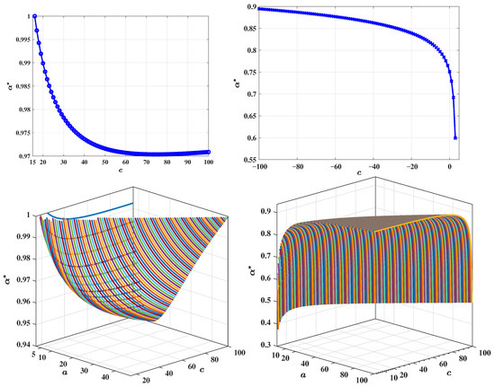
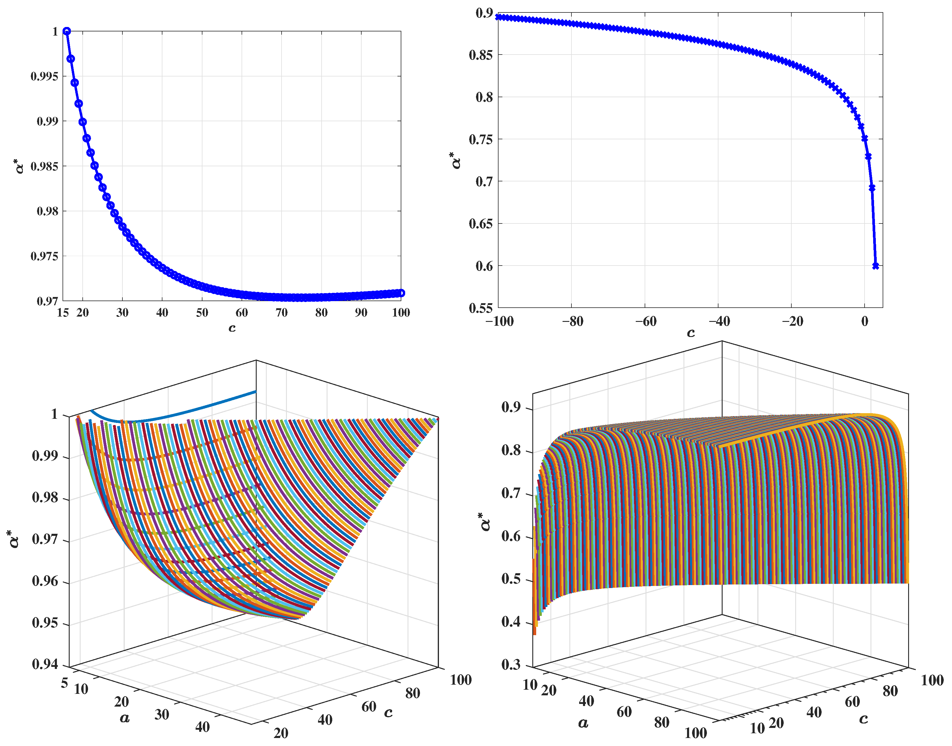
Since the first two coordinates of $E_1$ and $E_2$ have opposite signs while the third coordinate is identical, all eigenvalues of the Jacobian matrix at these equilibria coincide. Hence, their stability thresholds are the same. Next, we further explore the influence of parameters a and c on the critical fractional order $\alpha$* for $E_{1,2}$. Figure 1 illustrates the dependence of the critical order $\alpha$* on parameters a and c for both positive and negative values of b. The upper panels show the variation of $\alpha$* with respect to c for $b=2$ (left) and $b=-2$ (right), indicating that increasing c generally decreases the upper bound of $\alpha$*, thereby shrinking the stability region. The lower panels depict three-dimensional surfaces of $\alpha$* as function of both a and c, again for $b=2$ (left) and $b=-2$ (right). These results reveal the intricate interplay between system parameters and the fractional order in determining the stability boundary, and provide useful insights into controlling or suppressing chaotic behavior through appropriate adjustment of the fractional derivative order.

Figure 1. Critical order $\alpha$* at equilibria $E_{1,2}$ as a function of parameters a and c. (Upper) Variation of $\alpha$* with c for $a=4$, $b=2$ (left) and $b=-2$ (right). (Lower) Three-dimensional surfaces of ${\alpha }^{*}(a,c)$ for $b=2$ (left) and $b=-2$ (right).

3.3. Hopf Bifurcation with Respect to the Fractional Order

Theorem 2

(Hopf bifurcation condition, [34]). Let ρ denote a bifurcation parameter. For an equilibrium point $E_i$ of a three-dimensional fractional-order system, if the Jacobian matrix has one real eigenvalue ${\lambda }_1\left({\rho }^{*}\right)\ne 0$ and a pair of complex conjugate eigenvalues ${\lambda }_{2,3}\left({\rho }^{*}\right)$ at $\rho =\rho$*. Then the system undergoes Hopf bifurcation at $\rho =\rho$* if the following conditions hold:

1.

${\lambda }_1\left({\rho }^{*}\right)\ne 0$ and ${\displaystyle |arg\left({\lambda }_1\right)|\ne \frac{{\alpha }^{*}\pi }{2}}$;

2.

${\displaystyle |arg\left({\lambda }_2\right)| = |arg\left({\lambda }_3\right)|=\frac{{\alpha }^{*}\pi }{2}}$;

3.

${\displaystyle \frac{d}{d\rho }{|arg\left({\lambda }_i\right)|}_{\rho ={\rho }^{*}}\ne 0,i=2,3}$.

Now we verify that system (6) satisfies the three conditions listed in Theorem 2, thereby ensuring the occurrence of Hopf bifurcation.

As discussed in (3), the characteristic equation of the linearized system at $E_i$ is given by:

$$F(\lambda ,{\chi }_2,{\chi }_1,{\chi }_0)={\lambda }^3+{\chi }_2{\lambda }^2+{\chi }_1\lambda +{\chi }_0=0,$$

(10)

where ${\chi }_0=2ab(c-a),{\chi }_1=bc,{\chi }_2=a+b.$

Let $\lambda =r{e}^{i\theta }(r>0,\theta ={\displaystyle \frac{{\alpha }^{*}\pi }{2}})$ be a root of Equation (10). Substituting this into Equation (10) yields

$$r^3{e}^{i3\theta }+{\chi }_2{r}^2{e}^{i2\theta }+{\chi }_{1}r{e}^{i\theta }+{\chi }_0=0.$$

(11)

Separating (11) into real and imaginary parts gives

$$\left\{\begin{array}{c}{r}^{3}cos\left(3\theta \right)+{\chi }_2{r}^{2}cos\left(2\theta \right)+{\chi }_{1}rcos\theta +{\chi }_0=0,\hfill \\ r^{3}sin\left(3\theta \right)+{\chi }_2{r}^{2}sin\left(2\theta \right)+{\chi }_{1}rsin\theta =0.\hfill \end{array}\right.$$

(12)

By eliminating $r^3$ between the two equations and simplifying, we obtain two roots:

$${\displaystyle r_j=\frac{-{\chi }_{2}cos\theta \pm \sqrt{{\chi }_2^2{cos}^2\theta -{\chi }_1(4{cos}^2\theta -1)}}{4{cos}^2\theta -1},j=1,2,}$$

(13)

where $\theta \ne {\displaystyle \frac{\pi }{3}},{\alpha }^{*}\ne {\displaystyle \frac{2}{3}}$ and $\sqrt{{\chi }_2^2{cos}^2\theta -{\chi }_1(4{cos}^2\theta -1)}>0$.

To investigate the existence of Hopf bifurcation, we take c as the bifurcation parameter. From Equation (11), the critical value of c corresponding to the Hopf bifurcation is obtained as

$$c^h=-{\displaystyle \frac{1}{2ab}}(r^{3}cos\left(3\theta \right)+{\chi }_2{r}^{2}cos\left(2\theta \right)+{\chi }_{1}rcos\theta )+a,$$

where $|arg\left({\lambda }_{1,2}\left(c^h\right)\right)|={\displaystyle \frac{{\alpha }^{*}\pi }{2}}$, and ${\lambda }_{1,2}\left(c^h\right)$ are a pair of complex conjugate eigenvalues of Equation (11). It can be readily verified that Equation (11) also has a nonzero real root ${\lambda }_3\left(c^h\right)$ satisfying $|arg\left({\lambda }_3\left(c^h\right)\right)|\ne {\displaystyle \frac{{\alpha }^{*}\pi }{2}}$.

Let $\lambda \left(c\right)=u_1\left(c\right)+i{u}_2\left(c\right)$. Then $arg\left(\lambda \left(c\right)\right)=arctan{\displaystyle \frac{u_2\left(c\right)}{u_1\left(c\right)}}$, and

$${\displaystyle \frac{d}{dc}}{|arg\left(\lambda \left(c\right)\right)|}_{c=c^h}=\pm {\displaystyle \frac{1}{{\left|\lambda \left(c\right)\right|}^2}}\left|\begin{array}{cc}{u}_1\left(c\right)& u_2\left(c\right)\\ u_1^{\prime }\left(c\right)& u_2^{\prime }\left(c\right)\end{array}\right|.$$

Differentiating Equation (10) with respect to c yields

$${\displaystyle \frac{d\lambda \left(c\right)}{dc}=-\frac{b\lambda +2ab}{3{\lambda }^2\left(c\right)+2{\chi }_2\lambda \left(c\right)+{\chi }_1}.}$$

Substituting $\lambda =r_j{e}^{i\theta }$ at $c=c^h$, we have

$$\begin{array}{cc}\hfill {\displaystyle \frac{d\lambda \left(c\right)}{dc}}{|}_{c=c^h}& {\displaystyle =-\frac{b{r}_j(cos\theta +isin\theta )+2ab}{3r_j^2(cos\left(2\theta \right)+isin\left(2\theta \right))+2{\chi }_2{r}_j(cos\theta +isin\theta )+{\chi }_1}=\frac{-A+iB}{{\epsilon }_1^2+{\epsilon }_2^2},}\hfill \end{array}$$

where

$$\begin{array}{cc}\hfill & A={\epsilon }_1(b{r}_{j}cos\theta +2ab)+{\epsilon }_{2}b{r}_{j}sin\theta ,B={\epsilon }_2(b{r}_{j}cos\theta +2ab)-{\epsilon }_{1}b{r}_{j}sin\theta ,\hfill \\ \hfill & {\epsilon }_1=3r_j^{2}cos\left(2\theta \right)+2{\chi }_2{r}_{j}cos\theta +{\chi }_1,{\epsilon }_2=3r_j^{2}sin\left(2\theta \right)+2{\chi }_2{r}_{j}sin\theta .\hfill \end{array}$$

Hence

$$\left|\begin{array}{cc}{u}_1\left(c\right)& u_2\left(c\right)\\ u_1^{\prime }\left(c\right)& u_2^{\prime }\left(c\right)\end{array}\right|=\left|\begin{array}{cc}{r}_{j}cos\theta & r_{j}sin\theta \\ {\displaystyle \frac{-A}{{\epsilon }_1^2+{\epsilon }_2^2}}& {\displaystyle \frac{B}{{\epsilon }_1^2+{\epsilon }_2^2}}\end{array}\right|={\displaystyle \frac{r_j}{{\epsilon }_1^2+{\epsilon }_2^2}}(Bcos\theta +Asin\theta ),$$

where

$$\begin{array}{cc}\hfill Bcos\theta +Asin\theta & =cos\theta [{\epsilon }_2(b{r}_{j}cos\theta +2ab)-{\epsilon }_{1}b{r}_{j}sin\theta ]+sin\theta [{\epsilon }_1(b{r}_{j}cos+2ab)+{\epsilon }_{2}b{r}_{j}sin\theta ]\hfill \\ \hfill & =2ab({\epsilon }_{2}cos\theta +{\epsilon }_{1}sin\theta )+b{r}_j{\epsilon }_2.\hfill \end{array}$$

Since $r_j>0$ and $0<\theta ={\displaystyle \frac{{\alpha }^{*}\pi }{2}}<{\displaystyle \frac{\pi }{2}}$, we have ${\epsilon }_2=3r_j^{2}sin\left(2\theta \right)+2{\chi }_2{r}_{j}sin\theta >0$, implying $b{r}_j{\epsilon }_2>0$. From Ref. [34],

$${\epsilon }_{2}cos\theta +{\epsilon }_{1}sin\theta =2r_j^{2}sin\theta [r_j(4{cos}^2\theta -1)+{\chi }_{2}cos\theta ].$$

Using Equation (13), it follows that

$$r_j(4{cos}^2\theta -1)+{\chi }_{2}cos\theta =\pm \sqrt{{\chi }_2^2{cos}^2\theta -{\chi }_1(4{cos}^2\theta -1)}.$$

We now consider the two possible cases separately.

Case 1: If $r_j(4{cos}^2\theta -1)+{\chi }_{2}cos\theta =\sqrt{{\chi }_2^2{cos}^2\theta -{\chi }_1(4{cos}^2\theta -1)}$, then

$$\begin{array}{cc}\hfill 2ab({\epsilon }_{2}cos\theta +{\epsilon }_{1}sin\theta )+b{r}_j{\epsilon }_2& =4ab{r}_j^{2}sin\theta \sqrt{{\chi }_2^2{cos}^2\theta -{\chi }_1(4{cos}^2\theta -1)}+b{r}_j{\epsilon }_2>0.\hfill \end{array}$$

Hence,

$${\displaystyle \frac{d}{dc}{|arg\left(\lambda \left(c\right)\right)|}_{c=c^h}=\pm \frac{1}{r_j({\epsilon }_1^2+{\epsilon }_2^2)}(Bcos\theta +Asin\theta )\ne 0,}$$

thereby satisfying condition (3) of Theorem 2.

Case 2: If $r_j(4{cos}^2\theta -1)+{\chi }_{2}cos\theta =-\sqrt{{\chi }_2^2{cos}^2\theta -{\chi }_1(4{cos}^2\theta -1)}$, then

$$\begin{array}{cc}\hfill & 2ab({\epsilon }_{2}cos\theta +{\epsilon }_{1}sin\theta )+b{r}_j{\epsilon }_2\hfill \\ \hfill =& -4ab{r}_j^{2}sin\theta \sqrt{{\chi }_2^2{cos}^2\theta -{\chi }_1(4{cos}^2\theta -1)}+b{r}_j{\epsilon }_2\hfill \\ \hfill =& b{r}_j(3r_j^{2}sin\left(2\theta \right)+2{\chi }_2{r}_{j}sin\theta )-4ab{r}_j^{2}sin\theta \sqrt{{\chi }_2^2{cos}^2\theta -{\chi }_1(4{cos}^2\theta -1)}\hfill \\ \hfill =& 2b{r}_j^{2}sin\theta [3r_{j}cos\theta +{\chi }_2-2a\sqrt{{\chi }_2^2{cos}^2\theta -{\chi }_1(4{cos}^2\theta -1)}].\hfill \end{array}$$

To ensure that the above quantity is nonzero, it suffices that

$${\displaystyle \frac{2a\sqrt{{\chi }_2^2{cos}^2\theta -{\chi }_1(4{cos}^2\theta -1)}-{\chi }_2}{3cos\theta }\ne \frac{-{\chi }_{2}cos\theta -\sqrt{{\chi }_2^2{cos}^2\theta -{\chi }_1(4{cos}^2\theta -1)}}{4{cos}^2\theta -1}.}$$

Therefore, condition (3) of Theorem 2 also holds in this case.

For example, for parameter settings $a=4$, $b=2$, and $c=16.5$, we have from (9) that ${\lambda }_{2,3}=0.014\pm 5.76i$, $|arg\left({\lambda }_i\right)|={\displaystyle \frac{{\alpha }^{*}\pi }{2}}=1.5683$, and the critical order ${\alpha }^{*}=0.9984$. In this case, it implies $rcos\theta =0.014$ and $rsin\theta =5.76$. By computation, $r(Bcos\theta +Asin\theta )=43.20\ne 0$ for the term of ${\displaystyle \frac{d}{dc}}{|arg\left(\lambda \left(c\right)\right)|}_{c=c^h}$. Therefore, according to Theorem 2, the system (6) generates Hopf bifurcation at this critical point and is gradually becoming unstable. The corresponding numerical proofs will also be presented in Section 5.

4. Numerical Approximation of the Fractional System

4.1. Fast L1 Discretization and SOE Approximation

In this section, we propose an efficient time-stepping scheme for the fractional Lorenz-Stenflo system (6), together with fast implementation of the fractional derivative based on the sum-of-exponentials (SOE) technique. The stability of the resulting scheme is also established.

Let $T>0$ and ${\left\{t_k\right\}}_{k=0}^N$ be a uniform partition of $[0,T]$ with time step $h=T/N$. The classical L1 approximation [20] to discretize the Caputo derivative $D^{\alpha }u$ at $t=t_k$ is given by:

$$\begin{array}{cc}\hfill D^{\alpha }u\left(t_k\right)=& {\displaystyle \frac{1}{\Gamma (1-\alpha )}}{\displaystyle \sum _{j=0}^{k-1}}{\int }_{t_j}^{t_{j+1}}{\displaystyle \frac{u_s\left(s\right)}{{(t_k-s)}^{\alpha }}}ds\hfill \\ \hfill =& {\displaystyle \frac{1}{\Gamma (1-\alpha )}}{\displaystyle \sum _{j=0}^{k-1}}{\displaystyle \frac{u\left(t_{j+1}\right)-u\left(t_j\right)}{h}}{\int }_{t_j}^{t_{j+1}}{\displaystyle \frac{1}{{(t_k-s)}^{\alpha }}}ds+R^k\hfill \\ \hfill :=& L_t^{\alpha }u\left(t_k\right)+R^k,1\le k\le N,\hfill \end{array}$$

(14)

where $R^k$ is the corresponding local truncation error and $L_t^{\alpha }$ is defined by

$$L_t^{\alpha }u\left(t_k\right)={\displaystyle \frac{1}{d_{\alpha }}}[a_0^{\alpha }u\left(t_k\right)-{\displaystyle \sum _{j=1}^{k-1}}(a_{j-1}^{\alpha }-a_j^{\alpha })u\left(t_{k-j}\right)-a_{k-1}^{\alpha }u\left(t_0\right)],$$

with $d_{\alpha }=\Gamma (2-\alpha )h^{\alpha }$,

$$a_{k-j}^{\alpha }={\displaystyle \frac{1-\alpha }{h^{1-\alpha }}}{\int }_{t_{j-1}}^{t_j}{\displaystyle \frac{1}{{(t_k-s)}^{\alpha }}}ds={(k-j+1)}^{1-\alpha }-{(k-j)}^{1-\alpha }.$$

(15)

To improve readability, the superscript $\alpha$ in $a_{k-j}^{\alpha }$ will be omitted throughout the remainder of the paper whenever no ambiguity arises. The same convention applies to the notations $N_{\epsilon }^{\alpha }$, $s_i^{\alpha }$, ${\omega }_i^{\alpha }$, $U_i^{\alpha }\left(t_k\right)$, $U_i^{k,\alpha }$, and ${\widehat{a}}_{k-j}^{\alpha }$ introduced below, which will be written as $N_{\epsilon }$, $s_i$, ${\omega }_i$, $U_i\left(t_k\right)$, $U_i^k$, and ${\widehat{a}}_{k-j}$ respectively. The main coefficients and notations used in the numerical scheme are summarized in Table 1.

Table 1. The main coefficients and notations used in the numerical scheme.

$d_{\alpha }$	$\Gamma (2-\alpha )h^{\alpha }$
$a_{k-j}$	${(k-j+1)}^{1-\alpha }-{(k-j)}^{1-\alpha }$
$N_{\epsilon },s_i,{\omega }_i$	positive integers
${\widehat{a}}_{k-j}$	${\displaystyle \frac{1}{h}{\displaystyle \sum _{i=1}^{N_{\epsilon }}}\frac{{\omega }_i}{s_i}{e}^{-s_i(k-j)h}(1-e^{-s_{i}h})}$
$U_i^k$	${\displaystyle e^{-s_{i}h}{U}_i^{k-1}+\frac{1}{s_{i}h}{e}^{-s_{i}h}(1-e^{-s_{i}h})(u_{k-1}-u_{k-2}),U_i^1=0}$

Due to the intrinsic nonlocality of the standard L1 formula, its direct application results in a high computational complexity of $\mathcal{O}\left(N^2\right)$ and a storage cost of $\mathcal{O}\left(N\right)$. To alleviate this issue, we adopt a fast L1 formula based on the SOE technique [35], which approximates the kernel function ${(t_k-s)}^{-\alpha }$ in the time-fractional derivative and significantly reduces both computational and storage costs. In fact, it has been shown in [28,36] that for any $0<\alpha <1$ and prescribed absolute tolerance $\epsilon \ll 1$, there exists a positive integer $N_{\epsilon }$, positive quadrature nodes $s_i$ and weights ${\omega }_i$$(1\le i\le N_{\epsilon })$ such that

$${\displaystyle |\frac{1}{t^{\alpha }}-{\displaystyle \sum _{i=1}^{N_{\epsilon }}}{\omega }_i{e}^{-s_{i}t}|\le \epsilon ,t\in [h,T],}$$

with $0<h\ll 1$. The number of SOE terms $N_{\epsilon }$ satisfies

$${\displaystyle N_{\epsilon }=\mathcal{O}\left(log\frac{1}{\epsilon }\left(loglog\frac{1}{\epsilon }+log\frac{T}{h}\right)+log\frac{1}{h}\left(loglog\frac{1}{\epsilon }+log\frac{1}{h}\right)\right).}$$

Typically, for fixed $\epsilon ,N_{\epsilon }=\mathcal{O}(log\left(N\right))$ if $T\gg 1$;$N_{\epsilon }=\mathcal{O}\left({log}^2\left(N\right)\right)$ if $T\approx 1$.

To construct the fast L1 formula, the Caputo fractional derivative is decomposed into a local part and a history part. The local part is discretized using linear interpolation, while the history part is approximated by the SOE technique. Specifically,

$$\begin{array}{cc}\hfill D^{\alpha }u\left(t_k\right)=& {\displaystyle \frac{1}{\Gamma (1-\alpha )}}{\int }_{t_{k-1}}^{t_k}{\displaystyle \frac{u_s\left(s\right)}{{(t_k-s)}^{\alpha }}}ds+{\displaystyle \frac{1}{\Gamma (1-\alpha )}}{\int }_0^{t_{k-1}}{\displaystyle \frac{u_s\left(s\right)}{{(t_k-s)}^{\alpha }}}ds\hfill \\ \hfill \approx & {\displaystyle \frac{1}{\Gamma (1-\alpha )}}{\displaystyle \frac{u\left(t_k\right)-u\left(t_{k-1}\right)}{h}}{\int }_{t_{k-1}}^{t_k}{\displaystyle \frac{ds}{{(t_k-s)}^{\alpha }}}+{\displaystyle \frac{1}{\Gamma (1-\alpha )}}{\int }_0^{t_{k-1}}{\displaystyle \sum _{i=1}^{N_{\epsilon }}}{\omega }_i{e}^{-s_i(t_k-s)}{u}_s\left(s\right)ds\hfill \\ \hfill =& {\displaystyle \frac{u\left(t_k\right)-u\left(t_{k-1}\right)}{d_{\alpha }}}+{\displaystyle \frac{1}{\Gamma (1-\alpha )}}{\displaystyle \sum _{i=1}^{N_{\epsilon }}}{\omega }_i{U}_i\left(t_k\right),\hfill \end{array}$$

where

$$U_i\left(t_k\right)={\int }_0^{t_{k-1}}{e}^{-s_i(t_k-s)}{u}_s\left(s\right)ds,\mathrm{with}{U}_i\left(t_0\right)=0.$$

(16)

By employing a recursive formula and linear interpolation over the interval $(t_{k-2},t_{k-1})$, $U_i\left(t_k\right)$ can be approximated by

$$\begin{array}{cc}\hfill U_i\left(t_k\right)=& e^{-s_{i}h}{U}_i\left(t_{k-1}\right)+{\int }_{t_{k-2}}^{t_{k-1}}{e}^{-s_i(t_k-s)}{u}_s\left(s\right)ds\hfill \\ \hfill \approx & e^{-s_{i}h}{U}_i\left(t_{k-1}\right)+{\displaystyle \frac{u\left(t_{k-1}\right)-u\left(t_{k-2}\right)}{h}}{\int }_{t_{k-2}}^{t_{k-1}}{e}^{-s_i(t_k-s)}ds.\hfill \end{array}$$

(17)

By combining these results, we define the fast finite difference operator $F_t^{\alpha }$ as: for the discrete function ${\left\{u_k\right\}}_{k=0}^N$, for $1\le k\le N$,

$$F_t^{\alpha }{u}_k={\displaystyle \frac{u_k-u_{k-1}}{d_{\alpha }}}+{\displaystyle \frac{1}{\Gamma (1-\alpha )}}{\displaystyle \sum _{i=1}^{N_{\epsilon }}}{\omega }_i{U}_i^k,$$

(18)

where $U_i^k=e^{-s_{i}h}{U}_i^{k-1}+{\displaystyle \frac{u_{k-1}-u_{k-2}}{h}}{\int }_{t_{k-2}}^{t_{k-1}}{e}^{-s_i(t_k-s)}ds=e^{-s_{i}h}{U}_i^{k-1}+{\displaystyle \frac{1}{s_{i}h}}{e}^{-s_{i}h}(1-e^{-s_{i}h})(u_{k-1}-u_{k-2})$ with $U_i^1=0$ for $i=1,2,\cdots ,N_{\epsilon }$.

Consequently, it follows that

$$\begin{array}{cc}\hfill F_t^{\alpha }{u}_k=& {\displaystyle \frac{u_k-u_{k-1}}{d_{\alpha }}}+{\displaystyle \frac{1}{\Gamma (1-\alpha )}}{\displaystyle \sum _{i=1}^{N_{\epsilon }}}{\omega }_i{\displaystyle \sum _{j=1}^{k-1}}{\displaystyle \frac{u_j-u_{j-1}}{h}}{\int }_{t_{j-1}}^{t_j}{e}^{-s_i(t_k-s)}ds\hfill \\ \hfill =& {\displaystyle \frac{1}{\Gamma (1-\alpha )}}{\displaystyle \sum _{j=1}^k}{\widehat{a}}_{k-j}(u_j-u_{j-1})\hfill \\ \hfill =& {\displaystyle \frac{1}{\Gamma (1-\alpha )}}[{\widehat{a}}_0{u}_k-{\displaystyle \sum _{j=1}^{k-1}}({\widehat{a}}_{j-1}-{\widehat{a}}_j)u_{k-j}-{\widehat{a}}_{k-1}{u}_0],\hfill \end{array}$$

(19)

where

$$\begin{array}{cc}\hfill & {\widehat{a}}_0={\displaystyle \frac{1}{h}}{\int }_{t_{k-1}}^{t_k}{\displaystyle \frac{ds}{{(t_k-s)}^{\alpha }}}={\displaystyle \frac{h^{-\alpha }}{1-\alpha }},\hfill \\ \hfill & {\widehat{a}}_{k-j}={\displaystyle \frac{1}{h}}{\displaystyle \sum _{i=1}^{N_{\epsilon }}}{\omega }_i{\int }_{t_{j-1}}^{t_j}{e}^{-s_i(t_k-s)}ds={\displaystyle \frac{1}{h}}{\displaystyle \sum _{i=1}^{N_{\epsilon }}}{\displaystyle \frac{{\omega }_i}{s_i}}{e}^{-s_i(k-j)h}(1-e^{-s_{i}h}).\hfill \end{array}$$

(20)

The fast L1 scheme retains the accuracy of the standard L1 method while reducing the computational complexity from $\mathcal{O}\left(N^2\right)$ to $\mathcal{O}\left(N{N}_{\epsilon }\right)$ and the memory from $\mathcal{O}\left(N\right)$ to $\mathcal{O}\left(N_{\epsilon }\right)$, making it highly suitable for long-term simulations of fractional-order systems.

4.2. Semi-Implicit Numerical Scheme

The fast linear semi-implicit L1 scheme for (6) reads: given $(x_0,y_0,z_0)=(x\left(t_0\right),y\left(t_0\right),$$z\left(t_0\right))$, for $k=1,2,\cdots ,N$, find $(x_k,y_k,z_k)$, such that

$$\left\{\begin{array}{cc}\hfill F_t^{{\alpha }_1}{x}_k=& a(y_k-x_k),\hfill \\ \hfill F_t^{{\alpha }_2}{y}_k=& (c-a)x_k-a{x}_{k-1}{z}_k,\hfill \\ \hfill F_t^{{\alpha }_3}{z}_k=& x_{k-1}{y}_k-b{z}_k.\hfill \end{array}\right.$$

(21)

From (19), we have $F_t^{\alpha }{u}_k=(u_k-H_k^{\alpha })/d_{\alpha }$, where $H_k^{\alpha }=u_{k-1}-(1-\alpha )h^{\alpha }{\sum }_{i=1}^{N_{\epsilon }}{\omega }_i{U}_i^k$, then the scheme (21) can be decoupled as

$$\left\{\begin{array}{cc}\hfill y_k=& {\displaystyle \frac{H_k^{{\alpha }_2}+\frac{(c-a)d_{{\alpha }_2}}{1+a{d}_{{\alpha }_1}}{H}_k^{{\alpha }_1}-\frac{a{d}_{{\alpha }_2}}{1+b{d}_{{\alpha }_3}}{x}_{k-1}{H}_k^{{\alpha }_3}}{1-\frac{a(c-a)d_{{\alpha }_1}{d}_{{\alpha }_2}}{1+a{d}_{{\alpha }_1}}+\frac{a{d}_{{\alpha }_2}{d}_{{\alpha }_3}}{1+b{d}_{{\alpha }_3}}{\left(x_{k-1}\right)}^2}},\hfill \\ \hfill x_k=& {\displaystyle \frac{H_k^{{\alpha }_1}+a{d}_{{\alpha }_1}{y}_k}{1+a{d}_{{\alpha }_1}}},\hfill \\ \hfill z_k=& {\displaystyle \frac{H_k^{{\alpha }_3}+d_{{\alpha }_3}{x}_{k-1}{y}_k}{1+b{d}_{{\alpha }_3}}}.\hfill \end{array}\right.$$

(22)

4.3. Stability Analysis of the Scheme

To prove the stability of the proposed scheme (21), we first introduce several preliminary results. The analysis is based on deriving suitable bounds for the discrete convolution kernels and applying a discrete fractional Grönwall inequality. The properties of the discrete convolution kernels $\left\{{\widehat{a}}_j\right|0\le j\le k-1\}$ listed in Lemma 1 have been proved in [37]. In addition, an upper bound for the sum of these kernels is required, as stated in Lemma 2.

Lemma 1.

For $0<\alpha <1$, if the tolerance error of SOE satisfies $\epsilon <T^{-\alpha }$, the coefficients $\left\{{\widehat{a}}_j\right|0\le j\le k-1\}$ defined in (20) satisfy:

$${\widehat{a}}_1>{\widehat{a}}_2>\cdots >{\widehat{a}}_{k-1}>0.$$

Moreover, if ${\displaystyle \epsilon <\frac{2-2^{1-\alpha }}{1-\alpha }{h}^{-\alpha }}$, then

$${\widehat{a}}_0>{\widehat{a}}_1.$$

Lemma 2.

For $0<\alpha <1$, $k\ge 0$, the sum of the coefficients $\left\{{\widehat{a}}_j\right|0\le j\le k-1\}$ satisfy:

$$h{\displaystyle \sum _{j=0}^{k-1}}{\widehat{a}}_j\le {\displaystyle \frac{t_k^{1-\alpha }}{1-\alpha }}+\epsilon t_k.$$

(23)

Proof. 

See Appendix A. □

The following lemma provides a key inequality for the discrete fractional derivative. Together with the fractional discrete Grönwall inequality in Lemma 4, it serves as the main tool for establishing the stability result.

Lemma 3.

If the SOE tolerance $\epsilon <min\{T^{-\alpha },{\displaystyle \frac{2-2^{1-\alpha }}{1-\alpha }}{h}^{-\alpha }\}$, then for any mesh function $u=\left\{u_k\right|0\le k\le N\}$ defined on ${\left\{t_k\right\}}_{k=0}^N$, the following inequality holds: for $1\le n\le N$,

$$2\Gamma (1-\alpha )h{\displaystyle \sum _{k=1}^n}\left(F_t^{\alpha }{u}_k\right)u_k\ge h{\displaystyle \sum _{k=1}^n}{\widehat{a}}_{n-k}{\left(u_k\right)}^2-({\displaystyle \frac{t_n^{1-\alpha }}{1-\alpha }}+\epsilon t_n){\left(u_0\right)}^2.$$

(24)

Proof. 

See Appendix A. □

Lemma 4

([38]). Let the assumptions A1–A2 hold:

A1.

The discrete kernels ${\left\{A_k^{\left(n\right)}\right\}}_{k=0}^{n-1}$ are positive and monotone decreasing, that is,

$$A_0^{\left(n\right)}\ge A_1^{\left(n\right)}\ge \cdots \ge A_{n-1}^{\left(n\right)}>0,for1\le n\le N.$$

A2.

There is a constant ${\pi }_A>0$ such that the discrete kernels satisfy the lower bound

$$A_{n-k}^{\left(n\right)}\ge {\displaystyle \frac{1}{{\pi }_{A}h\Gamma (1-\alpha )}}{\int }_{t_{k-1}}^{t_k}{\displaystyle \frac{1}{{(t_n-s)}^{\alpha }}}dsfor1\le k\le n\le N.$$

Let ${\left\{g^n\right\}}_{n=1}^N$ and ${\left\{{\lambda }_l\right\}}_{l=0}^{N-1}$ be given non-negative sequences. Assume further that there exists a constant Λ such that ${\sum }_{l=0}^{N-1}{\lambda }_l\le \Lambda$, and that the time step size h satisfies

$$h\le {\displaystyle \frac{1}{\sqrt[\alpha ]{2{\pi }_A\Gamma (2-\alpha )\Lambda }}}.$$

Then, for any non-negative sequence ${\left\{v^k\right\}}_{k=0}^N$ such that

$${\displaystyle \sum _{k=1}^n}{A}_{n-k}^{\left(n\right)}(v^k-v^{k-1})\le {\displaystyle \sum _{k=1}^n}{\lambda }_{n-k}{v}^k+g^{n}for1\le n\le N,$$

(25)

it holds that

$$v^n\le 2E_{\alpha }(2{\pi }_A\Lambda t_n^{\alpha })(v^0+{\pi }_A\Gamma (1-\alpha )\underset{1\le j\le n}{max}\left\{t_j^{\alpha }{g}^j\right\}),$$

(26)

where $E_{\alpha }\left(t\right)$ is the Mittag–Leffler function defined by ${\displaystyle E_{\alpha }\left(t\right)={\displaystyle {\sum }_{k=0}^{\infty }}\frac{t^k}{\Gamma (1+k\alpha )}}$.

To apply Lemma 4, it is sufficient to verify that assumptions A1 and A2 are satisfied by the discrete kernels $\left\{{\widehat{a}}_{n-k}\right\}$. Lemma 1 implies that assumption A1 holds provided that the tolerance error $\epsilon$ satisfies $\epsilon <{\displaystyle \frac{2-2^{1-\alpha }}{1-\alpha }}{h}^{-\alpha }$. Moreover, assumption A2 holds with ${\pi }_A=3/2$ if $\epsilon \le {\displaystyle \frac{T^{-\alpha }}{3}}$. Indeed, note that

$$a_{n-k}={(n-k+1)}^{1-\alpha }-{(n-k)}^{1-\alpha }=(1-\alpha ){\xi }^{-\alpha }>(1-\alpha )N^{-\alpha }=(1-\alpha )T^{-\alpha }{h}^{\alpha },\xi \in (n-k,n-k+1),$$

by (A1), we derive

$$\begin{array}{cc}\hfill & {\widehat{a}}_{n-k}-{\displaystyle \frac{1}{{\pi }_{A}h\Gamma (1-\alpha )}}{\int }_{t_{k-1}}^{t_k}{\displaystyle \frac{1}{{(t_n-s)}^{\alpha }}}ds={\widehat{a}}_{n-k}-{\displaystyle \frac{2h^{-\alpha }}{3\Gamma (2-\alpha )}}{a}_{n-k}\hfill \\ \hfill \ge & {\displaystyle \frac{h^{-\alpha }}{1-\alpha }}(1-{\displaystyle \frac{2}{3\Gamma (1-\alpha )}})a_{n-k}-\epsilon >{\displaystyle \frac{h^{-\alpha }}{3(1-\alpha )}}{a}_{n-k}-\epsilon >{\displaystyle \frac{h^{-\alpha }}{3(1-\alpha )}}(1-\alpha )T^{-\alpha }{h}^{\alpha }-\epsilon \ge 0.\hfill \end{array}$$

Combining the above results, we are now in a position to establish the stability of the proposed scheme (21), as stated in the following theorem.

Theorem 3.

Let $a,b,c$ be positive constants, and assume that the time step size $h\le$${\displaystyle \frac{1}{\sqrt[{\alpha }_2]{3\Gamma (1-{\alpha }_2)\Gamma (2-{\alpha }_2)c^2/a}}}$, the SOE approximation error $\epsilon \le {min}_{i=1,2,3}\{{\displaystyle \frac{2-2^{1-{\alpha }_i}}{1-{\alpha }_i}}{h}^{-{\alpha }_i},{\displaystyle \frac{T^{-{\alpha }_i}}{3}}\}$. Then the discrete system (21) is stable; that is, for any $1\le n\le N$,

$$\begin{array}{cc}\hfill & {\displaystyle \frac{h}{\Gamma (1-{\alpha }_1)}}{\displaystyle \sum _{k=1}^n}{\widehat{a}}_{n-k}^{{\alpha }_1}{(x_k)}^2+{\displaystyle \frac{h}{\Gamma (1-{\alpha }_2)}}{\displaystyle \sum _{k=1}^n}{\widehat{a}}_{n-k}^{{\alpha }_2}{(y_k)}^2+{\displaystyle \frac{ah}{\Gamma (1-{\alpha }_3)}}{\displaystyle \sum _{k=1}^n}{\widehat{a}}_{n-k}^{{\alpha }_3}{(z_k)}^2\hfill \\ \hfill & +ah{\displaystyle \sum _{k=1}^n}{(x_k)}^2+h{\displaystyle \sum _{k=1}^n}{(y_k)}^2+2abh{\displaystyle \sum _{k=1}^n}{(z_k)}^2\hfill \\ \hfill \le & \left[6({\displaystyle \frac{c^2}{a}}+1){(\Gamma (1-{\alpha }_2))}^2{t}_n^{{\alpha }_2}{E}_{{\alpha }_2}({\displaystyle \frac{3c^2}{a}}\Gamma (1-{\alpha }_2)t_n^{{\alpha }_2})+2\right][{\displaystyle \frac{1}{2\Gamma (1-{\alpha }_1)}}({\displaystyle \frac{t_n^{1-{\alpha }_1}}{1-{\alpha }_1}}+\epsilon t_n){(x_0)}^2\hfill \\ \hfill & +{\displaystyle \frac{1}{2\Gamma (1-{\alpha }_2)}}({\displaystyle \frac{t_n^{1-{\alpha }_2}}{1-{\alpha }_2}}+\epsilon t_n){(y_0)}^2+{\displaystyle \frac{a}{2\Gamma (1-{\alpha }_3)}}({\displaystyle \frac{t_n^{1-{\alpha }_3}}{1-{\alpha }_3}}+\epsilon t_n){(z_0)}^2].\hfill \end{array}$$

(27)

Proof. 

Multiplying both sides of the discrete equations in (21) by $h{x}_k$, $h{y}_k$, and $ah{z}_k$ respectively, summing from $k=1$ to n, we deduce

$$\begin{array}{cc}\hfill & h{\displaystyle \sum _{k=1}^n}\left(F_t^{{\alpha }_1}{x}_k\right)x_k=ah{\displaystyle \sum _{k=1}^n}{x}_k{y}_k-ah{\displaystyle \sum _{k=1}^n}{\left(x_k\right)}^2,\hfill \\ \hfill & h{\displaystyle \sum _{k=1}^n}\left(F_t^{{\alpha }_2}{y}_k\right)y_k=(c-a)h{\displaystyle \sum _{k=1}^n}{x}_k{y}_k-ah{\displaystyle \sum _{k=1}^n}{x}_{k-1}{y}_k{z}_k,\hfill \\ \hfill & ah{\displaystyle \sum _{k=1}^n}\left(F_t^{{\alpha }_3}{z}_k\right)z_k=ah{\displaystyle \sum _{k=1}^n}{x}_{k-1}{y}_k{z}_k-abh{\displaystyle \sum _{k=1}^n}{\left(z_k\right)}^2.\hfill \end{array}$$

(28)

Let ${\displaystyle {\mathcal{X}}_n=h{\displaystyle \sum _{k=1}^n}{\widehat{a}}_{n-k}^{{\alpha }_1}{\left(x_k\right)}^2}$, ${\displaystyle {\mathcal{Y}}_n=h{\displaystyle \sum _{k=1}^n}{\widehat{a}}_{n-k}^{{\alpha }_2}{\left(y_k\right)}^2}$, ${\displaystyle {\mathcal{Z}}_n=h{\displaystyle \sum _{k=1}^n}{\widehat{a}}_{n-k}^{{\alpha }_3}{\left(z_k\right)}^2}$.By Lemma 3, summing up these equalities gives

$${\displaystyle \frac{{\mathcal{X}}_n}{2\Gamma (1-{\alpha }_1)}}+{\displaystyle \frac{{\mathcal{Y}}_n}{2\Gamma (1-{\alpha }_2)}}+{\displaystyle \frac{a{\mathcal{Z}}_n}{2\Gamma (1-{\alpha }_3)}}+ah{\displaystyle \sum _{k=1}^n}{(x_k)}^2+abh{\displaystyle \sum _{k=1}^n}{(z_k)}^2\le ch{\displaystyle \sum _{k=1}^n}{x}_k{y}_k+I_n,$$

(29)

where $I_n={\displaystyle \frac{1}{2\Gamma (1-{\alpha }_1)}}({\displaystyle \frac{t_n^{1-{\alpha }_1}}{1-{\alpha }_1}}+\epsilon t_n){(x_0)}^2+{\displaystyle \frac{1}{2\Gamma (1-{\alpha }_2)}}({\displaystyle \frac{t_n^{1-{\alpha }_2}}{1-{\alpha }_2}}+\epsilon t_n){(y_0)}^2+{\displaystyle \frac{a}{2\Gamma (1-{\alpha }_3)}}({\displaystyle \frac{t_n^{1-{\alpha }_3}}{1-{\alpha }_3}}+\epsilon t_n){(z_0)}^2$.

Using Young’s inequality, we get

$$c{x}_k{y}_k\le {\displaystyle \frac{a}{2}}{\left(x_k\right)}^2+{\displaystyle \frac{c^2}{2a}}{\left(y_k\right)}^2,$$

Substituting this inequality into (29) results in

$${\displaystyle \frac{{\mathcal{X}}_n}{2\Gamma (1-{\alpha }_1)}}+{\displaystyle \frac{{\mathcal{Y}}_n}{2\Gamma (1-{\alpha }_2)}}+{\displaystyle \frac{a{\mathcal{Z}}_n}{2\Gamma (1-{\alpha }_3)}}+{\displaystyle \frac{a}{2}}h{\displaystyle \sum _{k=1}^n}{\left(x_k\right)}^2+abh{\displaystyle \sum _{k=1}^n}{\left(z_k\right)}^2\le {\displaystyle \frac{c^2}{2a}}h{\displaystyle \sum _{k=1}^n}{\left(y_k\right)}^2+I_n.$$

(30)

Let ${\displaystyle Y_n=h{\displaystyle \sum _{k=1}^n}{\left(y_k\right)}^2}$, then

$${\mathcal{Y}}_n=h{\displaystyle \sum _{k=1}^n}{\widehat{a}}_{n-k}^{{\alpha }_2}{\left(y_k\right)}^2={\displaystyle \sum _{k=1}^n}{\widehat{a}}_{n-k}^{{\alpha }_2}(Y_k-Y_{k-1}),$$

(31)

it follows from (30) that

$${\displaystyle \sum _{k=1}^n}{\widehat{a}}_{n-k}^{{\alpha }_2}(Y_k-Y_{k-1})\le {\displaystyle \frac{\Gamma (1-{\alpha }_2)c^2}{a}}{Y}_n+2\Gamma (1-{\alpha }_2)I_n.$$

(32)

In virtue of the fractional discrete Grönwall inequality in Lemma 4, which we set $A_{n-k}^{\left(n\right)}={\widehat{a}}_{n-k}^{{\alpha }_2}$, $v^k=Y_k$, ${\lambda }_0={\displaystyle \frac{\Gamma (1-{\alpha }_2)c^2}{a}}$, ${\lambda }_1=\cdots ={\lambda }_{n-1}=0$, $g^n=2\Gamma (1-{\alpha }_2)I_n$ in (25), it holds

$$Y_n\le 6{(\Gamma (1-{\alpha }_2))}^2{t}_n^{{\alpha }_2}{I}_n{E}_{{\alpha }_2}\left({\displaystyle \frac{3c^2}{a}}\Gamma (1-{\alpha }_2)t_n^{{\alpha }_2}\right).$$

(33)

Plugging (33) into the right side of (30), we obtain

$$\begin{array}{cc}\hfill & {\displaystyle \frac{{\mathcal{X}}_n}{\Gamma (1-{\alpha }_1)}}+{\displaystyle \frac{{\mathcal{Y}}_n}{\Gamma (1-{\alpha }_2)}}+{\displaystyle \frac{a{\mathcal{Z}}_n}{\Gamma (1-{\alpha }_3)}}+ah{\displaystyle \sum _{k=1}^n}{\left(x_k\right)}^2+2abh{\displaystyle \sum _{k=1}^n}{\left(z_k\right)}^2\hfill \\ \hfill \le & \left[{\displaystyle \frac{6c^2}{a}}{(\Gamma (1-{\alpha }_2))}^2{t}_n^{{\alpha }_2}{E}_{{\alpha }_2}({\displaystyle \frac{3c^2}{a}}\Gamma (1-{\alpha }_2)t_n^{{\alpha }_2})+2\right]I_n.\hfill \end{array}$$

(34)

Combining (34) and (33) yields the desired estimate (27), which completes the proof. □

5. Numerical Examples

This section presents numerical experiments to investigate the dynamical behavior of the fractional-order T system (6) using the proposed numerical scheme (21). The results illustrate various dynamical features, including Lyapunov exponents, time series, phase portraits, and bifurcation structures, and also demonstrate the effectiveness of the scheme in capturing long-time dynamics.

The stability of the scheme is guaranteed under the conditions in Theorem 3, which constrain the time step size h and the SOE tolerance $\epsilon$. In practice, these conditions are sufficient but not necessarily sharp. In the following simulations, we set $\epsilon \le {10}^{-10}$ and $0.001\le h\le 0.05$. Although the chosen time step sizes may exceed the theoretical bound in certain cases, the numerical results remain stable and consistent with the theoretical analysis.

5.1. Lyapunov Exponents Analysis

Lyapunov exponents(LEs) provide a quantitative measure of the stability and long-term behavior of dynamical systems. While several well-established algorithms exist for integer-order systems, these methods are generally not directly applicable to fractional-order systems due to the intrinsic nonlocality of fractional derivatives.

To account for this nonlocality, we adapt the computational approach proposed in [39], which was originally developed for Grünwald–Letnikov derivatives and explicit discretizations. Since our system involves the Caputo fractional derivative and a semi-implicit scheme, the algorithm is modified to be consistent with the discrete formulation (21). The main steps of the adapted procedure are outlined below.

The fast scheme (22) can be written in vector form as

$$\mathit{x}\left(t_k\right)=\mathit{F}(\mathit{x}\left(t_{k-1}\right),\mathit{x}\left(t_{k-2}\right),\cdots ,\mathit{x}\left(t_0\right)),$$

where $\mathbf{x}={(x,y,z)}^T$, and $\mathit{F}$ is the vector-valued mapping determined by the discrete scheme. The deviation due to an initial perturbation ${\mathit{w}}^{\left(0\right)}=(w_1^{\left(0\right)},w_2^{\left(0\right)},w_3^{\left(0\right)})$ evolves as

$${\mathit{w}}^{\left(k\right)}={\mathit{J}}_F^{(k-1)}{\mathit{w}}^{(k-1)}=\cdots ={\displaystyle \prod _{i=0}^{k-1}}{\mathit{J}}_F^{\left(i\right)}{\mathit{w}}^{\left(0\right)}={\mathit{A}}^{\left(k\right)}{\mathit{w}}^{\left(0\right)}={\displaystyle \sum _{i=1}^3}{\mathit{a}}_i^{\left(k\right)}{w}_i^{\left(0\right)},$$

(35)

where ${\mathit{A}}^{\left(k\right)}$ is the tangent map at step k and ${\mathit{a}}_i^{\left(k\right)}$ denotes its i-th column. Taking three sets of initial perturbation ${\mathit{W}}^{\left(0\right)}=\mathrm{diag}({\epsilon }_1,{\epsilon }_2,{\epsilon }_3)$, ${\epsilon }_i\ne 0$, we obtain

$${\mathit{W}}^{\left(k\right)}={\mathit{A}}^{\left(k\right)}{\mathit{W}}^{\left(0\right)}.$$

Since ${\mathit{J}}_F^{(k-1)}$ in (35) cannot be computed directly due to nonlocality, we derive recurrence relations for ${\mathit{A}}^{\left(k\right)}$. It’s clear that the semi-implicit scheme (21) can be rewritten as

$$\left\{\begin{array}{cc}\hfill x_k=& {\displaystyle \frac{a{d}_{{\alpha }_1}{y}_k+H_k^{{\alpha }_1}}{1+a{d}_{{\alpha }_1}}},\hfill \\ \hfill y_k=& d_{{\alpha }_2}[(c-a)x_k-a{x}_{k-1}{z}_k]+H_k^{{\alpha }_2},\hfill \\ \hfill z_k=& {\displaystyle \frac{d_{{\alpha }_3}{x}_{k-1}{y}_k+H_k^{{\alpha }_3}}{1+b{d}_{{\alpha }_3}}}.\hfill \end{array}\right.$$

(36)

The perturbation equations are then

$$\left\{\begin{array}{cc}\hfill \delta x_k=& {\displaystyle \frac{a{d}_{{\alpha }_1}\delta y_k+\delta H_k^{{\alpha }_1}}{1+a{d}_{{\alpha }_1}}},\hfill \\ \hfill \delta y_k=& d_{{\alpha }_2}[(c-a)\delta x_k-a{z}_k\delta x_{k-1}-a{x}_{k-1}\delta z_k]+\delta H_k^{{\alpha }_2},\hfill \\ \hfill \delta z_k=& {\displaystyle \frac{d_{{\alpha }_3}(y_k\delta x_{k-1}+x_{k-1}\delta y_k)+\delta H_k^{{\alpha }_3}}{1+b{d}_{{\alpha }_3}}},\hfill \end{array}\right.$$

where $\delta H_k^{{\alpha }_i}$ represents the perturbation terms generated from historical items $H_k^{{\alpha }_i},i=1,2,3$ based on the SOE convolutions.

The coefficients of the tangent matrix ${\mathit{A}}^{\left(k\right)}={\left(a_{m,j}^{\left(k\right)}\right)}_{3\times 3}$ satisfy

$$\left\{\begin{array}{cc}\hfill a_{2,j}^{\left(k\right)}=& {\displaystyle \frac{-a{d}_{{\alpha }_2}(\frac{d_{{\alpha }_3}}{1+b{d}_{{\alpha }_3}}{x}_{k-1}{y}_k+z_k)a_{1,j}^{(k-1)}+\frac{(c-a)d_{{\alpha }_2}}{1+a{d}_{{\alpha }_1}}{\left(A{H}_{{\alpha }_1}\right)}_j^k+{\left(A{H}_{{\alpha }_2}\right)}_j^k-\frac{a{d}_{{\alpha }_2}{x}_{k-1}}{1+b{d}_{{\alpha }_3}}{\left(A{H}_{{\alpha }_3}\right)}_j^k}{1-\frac{a(c-a)d_{{\alpha }_1}{d}_{{\alpha }_2}}{1+a{d}_{{\alpha }_1}}+\frac{a{d}_{{\alpha }_2}{d}_{{\alpha }_3}}{1+b{d}_{{\alpha }_3}}{\left(x_{k-1}\right)}^2}},\hfill \\ \hfill a_{1,j}^{\left(k\right)}=& {\displaystyle \frac{a{d}_{{\alpha }_1}{a}_{2,j}^{\left(k\right)}+{\left(A{H}_{{\alpha }_1}\right)}_j^k}{1+a{d}_{{\alpha }_1}}},\hfill \\ \hfill a_{3,j}^{\left(k\right)}=& {\displaystyle \frac{d_{{\alpha }_3}(y_k{a}_{1,j}^{(k-1)}+x_{k-1}{a}_{2,j}^{\left(k\right)})+{\left(A{H}_{{\alpha }_3}\right)}_j^k}{1+b{d}_{{\alpha }_3}}},\hfill \end{array}\right.$$

with the auxiliary terms

$$\begin{array}{cc}\hfill & {\left(A{H}_{{\alpha }_l}\right)}_j^k=a_{l,j}^{(k-1)}-(1-{\alpha }_l)h^{{\alpha }_l}{\displaystyle \sum _{i=1}^{N_{\epsilon }}}{\omega }_i{\left(A{U}_i^k\right)}_{l,j},\hfill \\ \hfill & {\left(A{U}_i^k\right)}_{l,j}=e^{-s_{i}h}{\left(A{U}_i^{k-1}\right)}_{l,j}+{\displaystyle \frac{1}{s_{i}h}}{e}^{-s_{i}h}(1-e^{-s_{i}h})(a_{l,j}^{(k-1)}-a_{l,j}^{(k-2)}),j,l=1,2,3.\hfill \end{array}$$

The LEs are finally computed as

$${\lambda }_j=\underset{t_k\to \infty }{lim}{\displaystyle \frac{1}{t_k}}ln{\displaystyle \frac{\parallel {\mathit{w}}_j^{\left(k\right)}\parallel }{\parallel {\mathit{w}}_j^{\left(0\right)}\parallel }}=\underset{k\to \infty }{lim}{\displaystyle \frac{1}{kh}}ln{\displaystyle \frac{|{\epsilon }_j|\parallel {\mathit{a}}_j^{\left(k\right)}\parallel }{\parallel {\mathit{w}}_j^{\left(0\right)}\parallel }}=\underset{k\to \infty }{lim}{\displaystyle \frac{1}{kh}}ln\parallel {\mathit{a}}_j^{\left(k\right)}\parallel ,j=1,2,3.$$

To prevent numerical divergence, we apply Gram–Schmidt orthonormalization every N steps, with the orthonormalization timestep be $h_{\mathrm{norm}}=Nh$. In practice, we set $h_{\mathrm{norm}}=10h$.

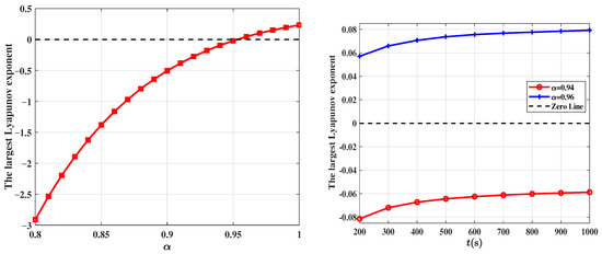
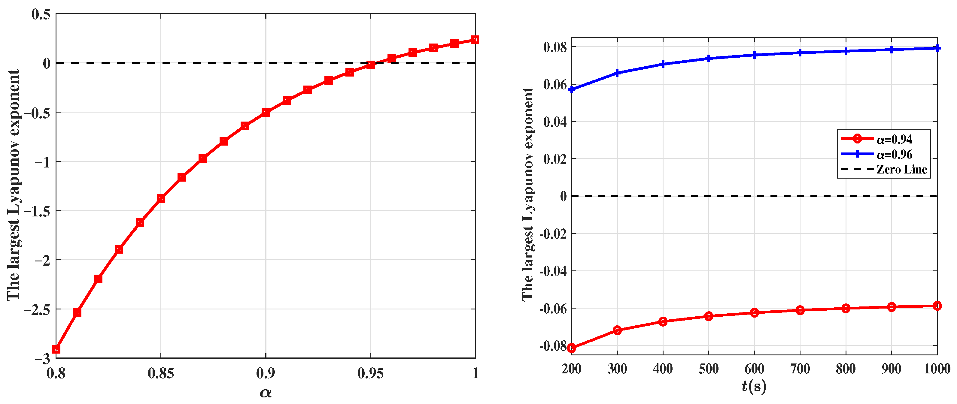
For validation, we consider the commensurate case (${\alpha }_1={\alpha }_2={\alpha }_3=\alpha$) with parameters $a=2$, $b=0.5$, $c=18$. The two nontrivial equilibrium points are $E_1(2,2,8)$, $E_2(-2,-2,8)$. Since $b(2a^2+bc-ac)=-9.5<0$, the integer-order system is unstable, whereas the fractional system remains stable when $\alpha <{\alpha }^{*}<0.9487$. We set $h=0.001$, SOE tolerance $\epsilon ={10}^{-10}$, and initial condition $(x_0,y_0,z_0)=(2,2,8)$. The largest Lyapunov exponent ${\lambda }_{\max }$ as a function of $\alpha$ is shown in Figure 2 (left). Figure 2 (right) presents the temporal evolution of ${\lambda }_{\max }$ for $\alpha =0.94$ and $\alpha =0.96$. These results confirm that ${\lambda }_{\max }<0$ for $\alpha \le 0.94$ and becomes positive for $\alpha >0.94$, which is consistent with the theoretical stability threshold.

Figure 2. For parameters $a=2$, $b=0.5$, $c=18$. (Left) The largest Lyapunov exponent ${\lambda }_{\max }$ as function of the fractional order $\alpha$ ($T=100$, the disturbance ${\epsilon }_1={\epsilon }_2={\epsilon }_3=0.05$). (Right) Time evolution of ${\lambda }_{\max }$ for $\alpha =0.94,0.96$ (${\epsilon }_1={\epsilon }_2={\epsilon }_3=0.01$).

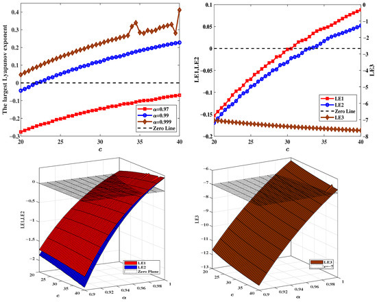
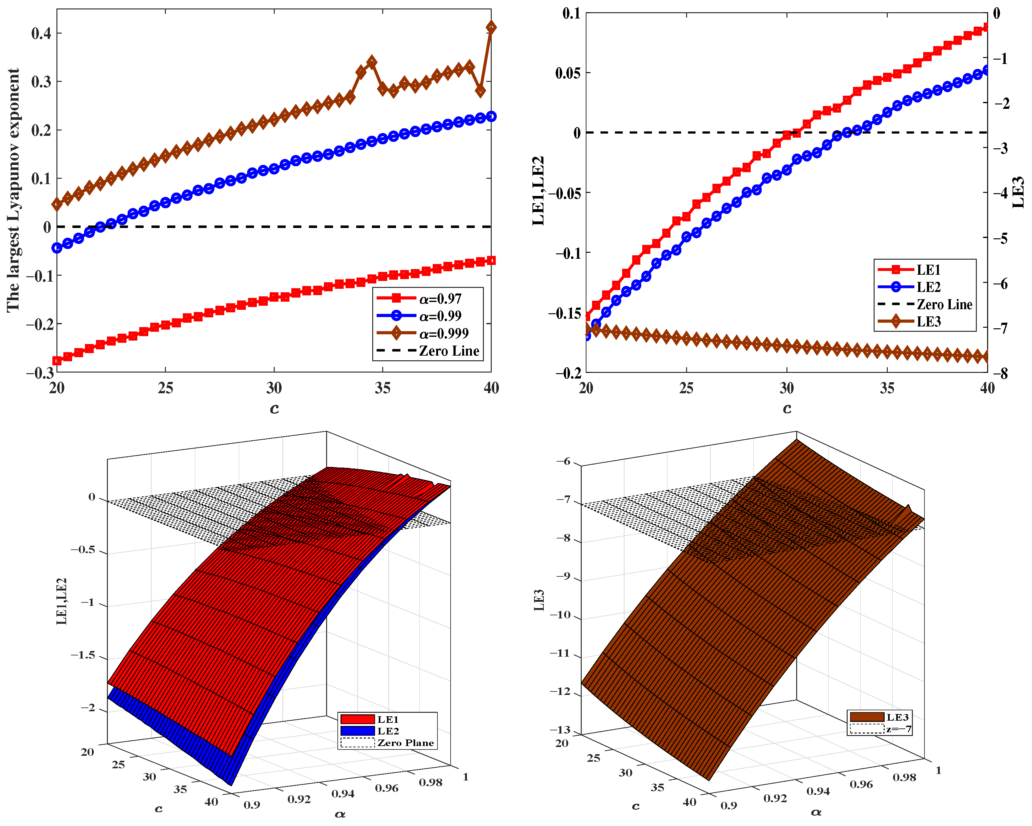
We further investigate the influence of the parameter c and the fractional order $\alpha$ on the LEs with $a=4,b=2$, as shown in Figure 3. (i) In the upper-left panel, the largest Lyapunov exponent is plotted as a function of c for different $\alpha$. The exponent remains negative across the tested range of c for $\alpha =0.97$, confirming stability. While for $\alpha =0.999$, it becomes positive, indicating transition to chaos. (ii) The upper-right panel shows all three LEs for $\alpha =0.98$. Both the first and second exponents gradually cross zero as c increases, implying a decreasing stability threshold $\alpha$*. This is consistent with the trend reported in Figure 1 (upper right). (iii) The lower panels show the three-dimensional surfaces of the LEs as functions of both $\alpha$ and c. The left plot presents the largest and second exponents with the zero-plane reference, while the right plot displays the third exponent with a baseline at $-7$, clearly illustrating the evolution of the stability regions with respect to the fractional order and system parameters. As can be seen from the figure, under certain parameter conditions, two Lyapunov exponents are greater than zero, indicating that the system is in a state of superchaotic oscillation.

Figure 3. LEs as functions of the fractional order $\alpha$ and the parameter c for $a=4$ and $b=2$. (Upper panels, 2D) Left: the largest lyapunov exponent versus c for different values of $\alpha$. Right: All three LEs at $\alpha =0.98$. (Lower panels, 3D) Left: surfaces of the largest and second LEs with the zero-plane reference; Right: surface of the third LE with a baseline at $-7$.

5.2. Time and Phase Diagrams

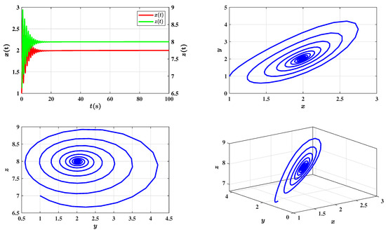
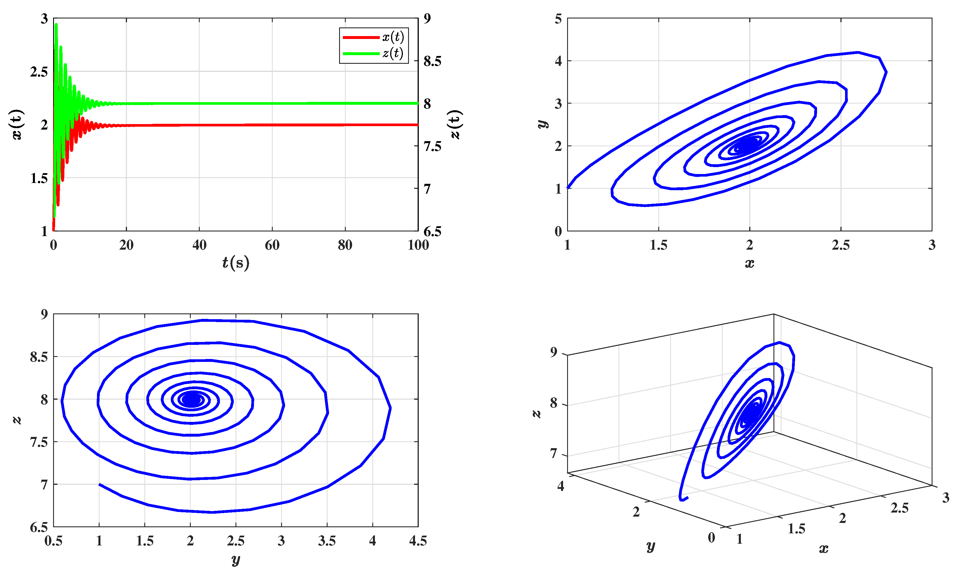
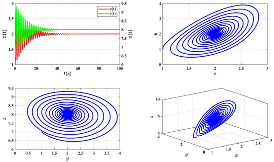
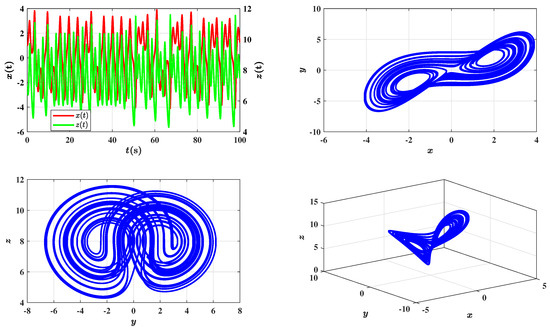
We continue with the same parameter setting as in Section 5.1, namely $a=2$, $b=0.5$, and $c=18$, for which the theoretical stability threshold satisfies ${\alpha }^{*}<0.9487$. The SOE tolerance is set to $\epsilon ={10}^{-10}$, and the initial condition is $(x_0,y_0,z_0)=(1,1,7)$. Figure 4, Figure 5 and Figure 6 display the numerical solutions and phase portraits of the fractional T system for three sets of fractional orders:

Figure 4. The approximate solution $x,y,z$ and phase diagram over time for the fractional T system by fast scheme (21) with $a=2$, $b=0.5$, $c=18$, ${\alpha }_1=0.7,{\alpha }_2=0.8,{\alpha }_3=0.9$, $T=100,h=0.05$.

Figure 5. The approximate solution $x,y,z$ and phase diagram over time for the fractional T system by fast scheme (21) with $a=2$, $b=0.5$, $c=18$, ${\alpha }_1=0.9,{\alpha }_2=0.92,{\alpha }_3=0.94$, $T=100,h=0.002$.

Figure 6. The approximate solution $x,y,z$ and phase diagram over time for the fractional T system by fast scheme (21) with $a=2$, $b=0.5$, $c=18$, ${\alpha }_1=0.97,{\alpha }_2=0.98,{\alpha }_3=0.99$, $T=100,h=0.002$.

(i) $({\alpha }_1,{\alpha }_2,{\alpha }_3)=(0.7,0.8,0.9)$, (ii) $(0.9,0.92,0.94)$, (iii) $(0.97,0.98,0.99)$.

Cases (i) and (ii) exhibit asymptotic convergence to equilibrium, while case (iii) produces a chaotic attractor. Moreover, a comparison between Figure 4 and Figure 5 shows that it takes longer to reach a steady state as the fractional orders approach the critical value, reflecting the memory-induced damping effect characteristic of fractional dynamics.

Compared with the classical integer-order T system (see Figure 2b in [18]), which displays a single-mode response under the same parameter settings, the fractional T system demonstrates a broader spectrum of dynamic behaviors, ranging from equilibrium to periodic motion and chaos as the fractional orders vary. A smaller fractional order tends to suppress bifurcation and destabilization, implying that adjusting the fractional order may serve as an effective control mechanism for attenuating chaotic oscillations in practical applications.

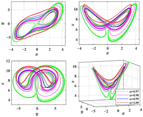
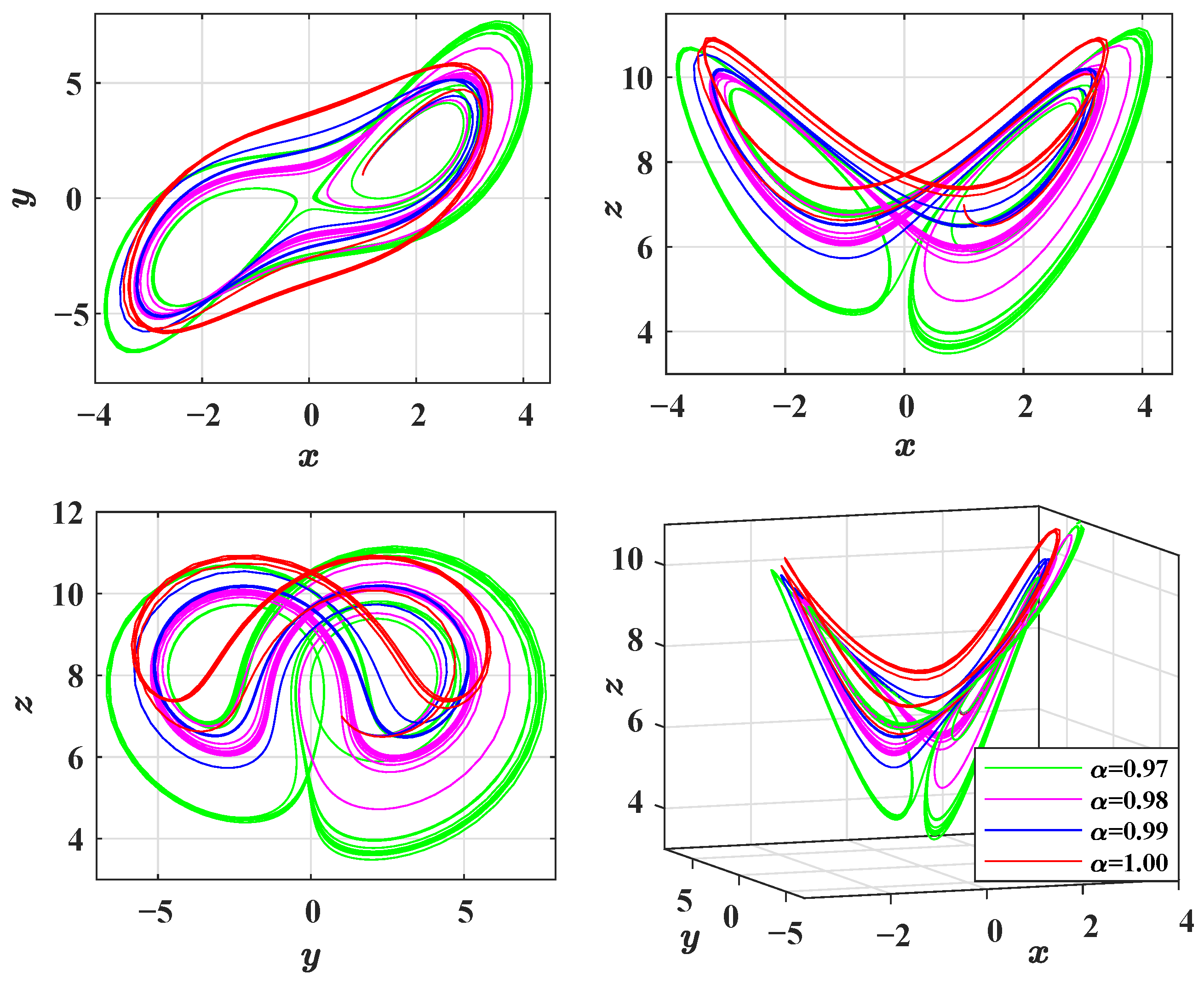
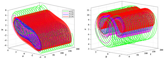
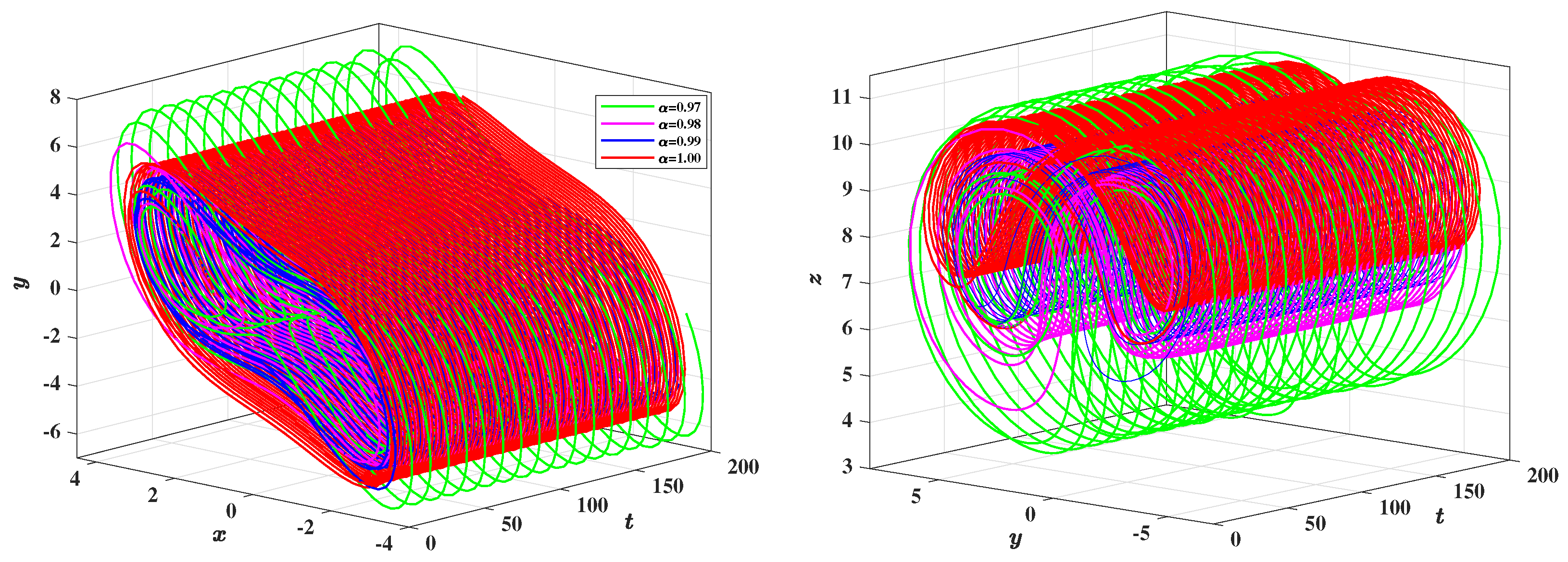
Figure 7 further illustrates the geometric evolution of attractors under $\alpha =0.97,0.98,$ 0.99, 1, projected onto the x-y, y-z, x-z planes as well as in three dimensions. As $\alpha$ increases, the attractor is increasingly contracting, which may be the influence of fractional order genetic memory. Figure 8 displays the temporal projections of $x\left(t\right),y\left(t\right)$ and $y\left(t\right),z\left(t\right)$, where a quasi-periodic structure is observed; the oscillations exhibit near-periodicity but vary in amplitude, indicating that the chaotic phenomenon of the system may develop from the periodic cycle caused by Hopf bifurcation.

Figure 7. Chaotic attractors of the fractional T system (21) for different fractional orders, with $a=2$, $b=0.5$, $c=18$. (Upper, left) Projection onto the x-y plane. (Upper, right) Projection onto the x-z plane. (Lower, left) Projection onto the y-z plane. (Lower, right) Three-dimensional phase portrait.

Figure 8. Three-dimensional trajectory projections of the fractional T system (21) for different fractional orders, with $a=2$, $b=0.5$, $c=18$. (Left) Projection in the x-y-t space. (Right) Projection in the y-z-t space.

To demonstrate the computational advantages of the propsed fast L1 scheme, we compare it against the classical L1 method and the Grünwald–Letnikov ( abbreviated as GL) schemes. The GL approximation takes the form [32]:

$$D^{\alpha }u\left(t_n\right)\approx {\displaystyle \sum _{j=0}^n}{c}_j^{\alpha }u\left(t_{n-j}\right),c_0^{\alpha }=h^{-\alpha },c_j^{\alpha }=(1-{\displaystyle \frac{1+\alpha }{j}})c_{j-1}^{\alpha },j\ge 1.$$

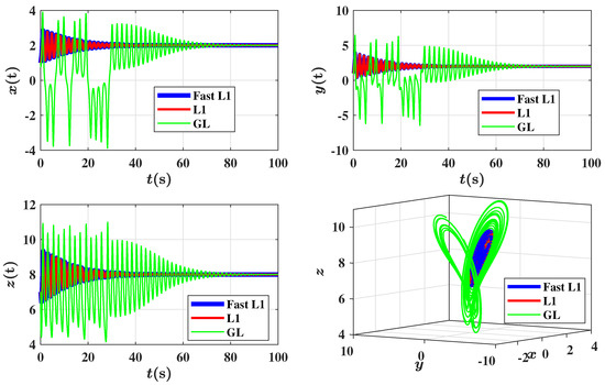
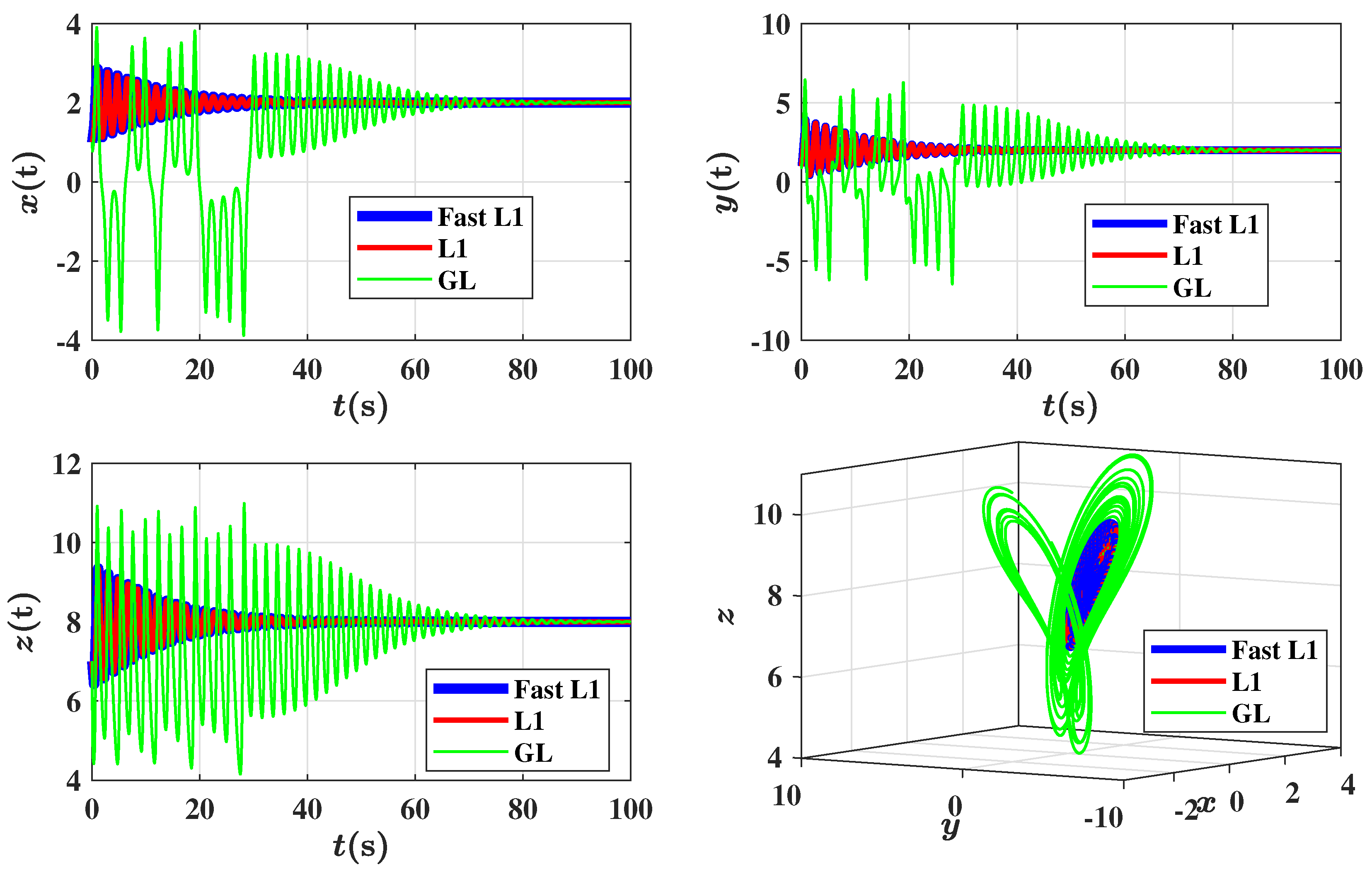
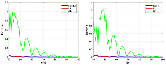
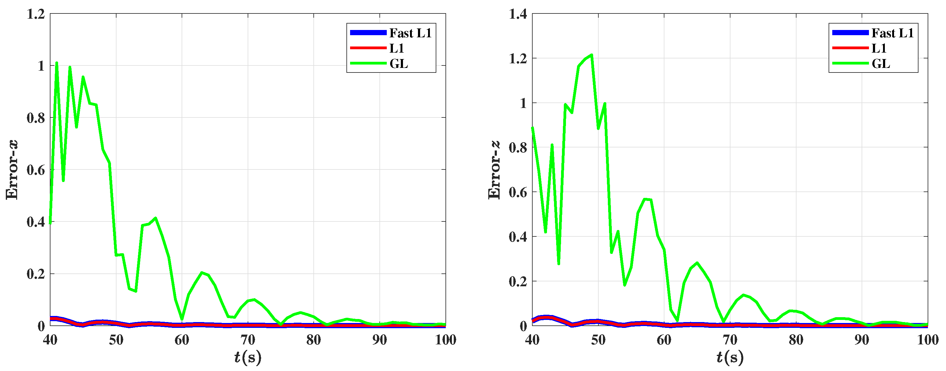
For $a=2$, $b=0.5$, $c=18$, $h=0.002$, and $\alpha =0.93$, Figure 9 shows the numerical solutions obtained by the three schemes, and Figure 10 presents the error curves of $x\left(t\right)$ and $z\left(t\right)$. The results indicate that the fast and standard L1 schemes produce nearly identical solution trajectories, whereas the GL scheme exhibits larger oscillations, suggesting a lower approximation accuracy compared with the fast and standard L1 methods.

Figure 9. The evolution of numerical solutions over time of three schemes: fast L1 scheme, L1 scheme, GL scheme with $\alpha =0.93$, $h=0.002$, $T=100$ and $a=2$, $b=0.5$, $c=18$.

Figure 10. Comparison of the errors of the three schemes for x (left) and z (right) with $\alpha =0.93$, $h=0.002$, $T=100$ and $a=2$, $b=0.5$, $c=18$.

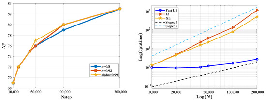
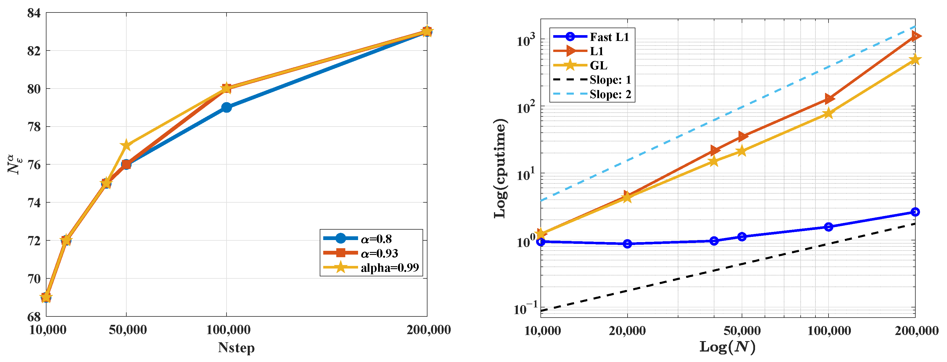
Moreover, the left panel of Figure 11 displays the number of SOE terms $N_{\epsilon }^{\alpha }$ required for different time step sizes. Even as h decreases from $0.1$ to $0.005$, $N_{\epsilon }^{\alpha }$ increases only slightly from 69 to 83 (when $\alpha =0.93$), whereas the classical L1 scheme must store all historical values. The right panel of Figure 11 shows that the CPU time for the fast L1 scheme grows approximately linearly with $\mathrm{Log}\left(N\right)$, in contrast to the quadratic growth observed for the classical L1 and GL schemes. These comparisons clearly demonstrate that the proposed fast L1 method achieves significantly reduced computational cost while retaining the same numerical accuracy, making it well-suited for long-time simulations of fractional-order dynamical systems.

Figure 11. (Left) SOE number $N_{\epsilon }^{\alpha }$ versus the total time steps for different $\alpha$, $T=1000$, $\epsilon ={10}^{-12}$. (Right) CPU (in seconds) for the three schemes as a function of the total time steps, $\alpha =0.93$, $T=1000$, $\epsilon ={10}^{-12}$.

5.3. Bifurcation Analysis

To compare with the fractional-order dynamics, we also examine the bifurcation behavior of the integer-order T system. Using the forward Euler discretization, the discrete form of T system (1) is given by

$$\left\{\begin{array}{c}x\to x+\delta \left(a\right(y-x\left)\right),\hfill \\ y\to y+\delta \left(\right(c-a)x-axz),\hfill \\ z\to z+\delta (xy-bz),\hfill \end{array}\right.$$

(37)

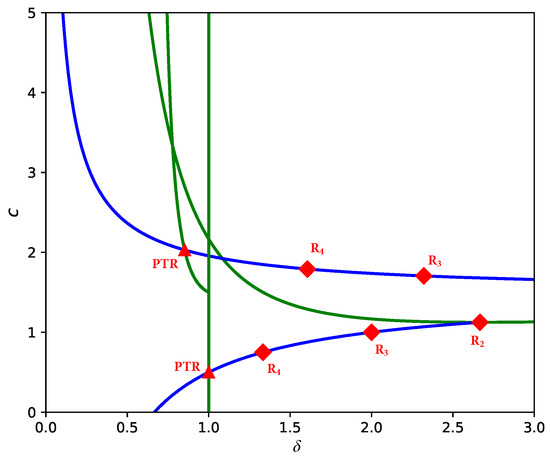
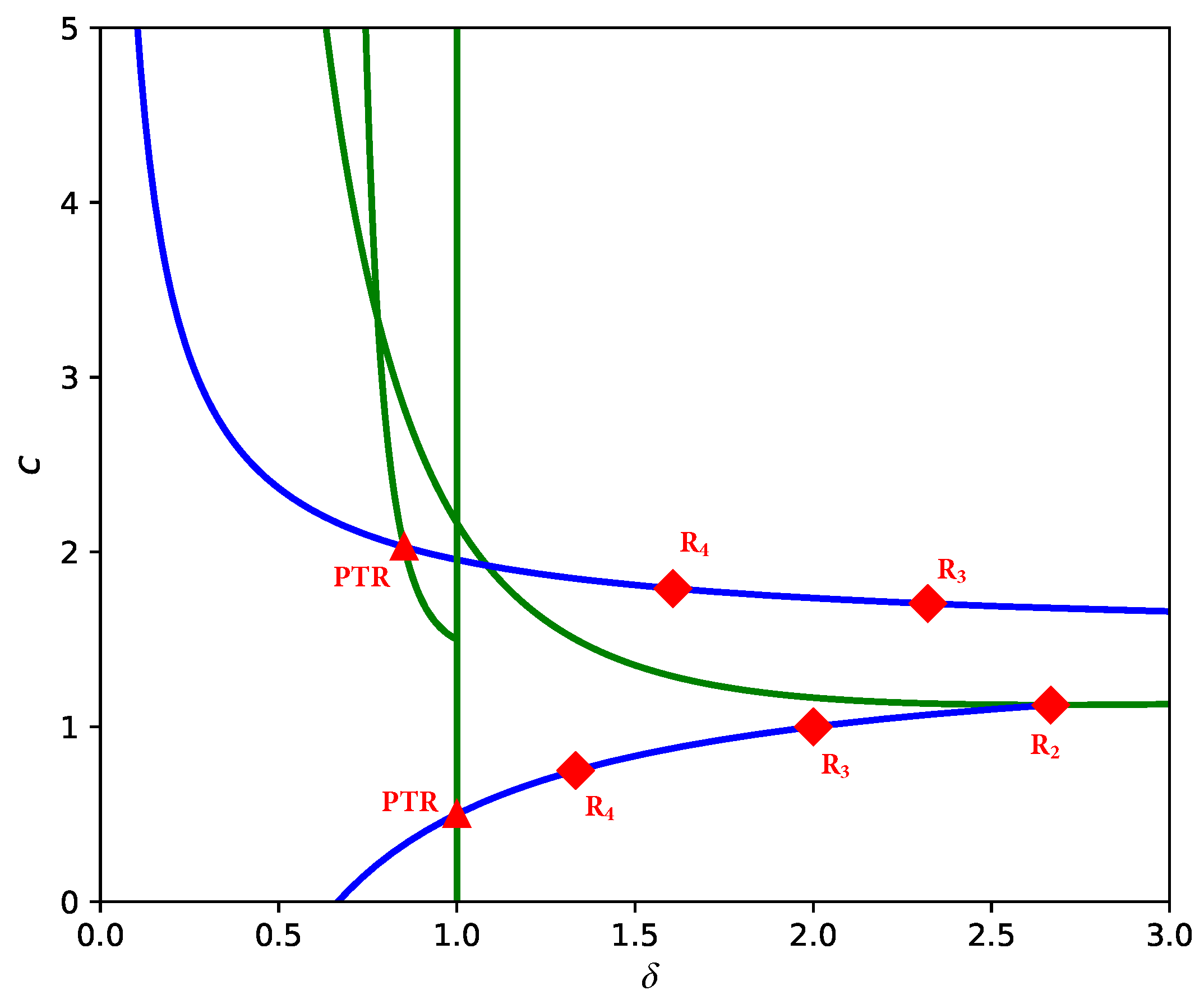
where $\delta >0$ is the time-step parameter. Taking $a=1.5$, $b=2$ and initial condition $(0,0,0)$, we consider c and $\delta$ as bifurcation parameters. The corresponding two-parameter bifurcation diagram is displayed in Figure 12, which shows the bifurcation structure of the integer-order T system and serves as a baseline for comparison with its fractional-order counterpart. The green curve corresponds to the period-doubling bifurcation, while the blue curve represents the Neimark–Sacker bifurcation. Their intersections form period-doubling and torus (abbreviated as PTR) points, at which the characteristic equation has one eigenvalue equal to $-1$ and a pair of complex conjugate eigenvalues on the unit circle (mode 1). Two such PTR points are identified at $(\delta ,c)=(1,0.5)$ and $(0.9,2.0029)$. The diagram also contains the resonance points R₂, R₃ and R₄, corresponding to $1:2$, $1:3$ and $1:4$ resonances, with eigenvalues $-1$, ${\displaystyle \frac{1}{2}}\pm {\displaystyle \frac{\sqrt{3}}{2}}i$ and ${\displaystyle \frac{\sqrt{2}}{2}}\pm {\displaystyle \frac{\sqrt{2}}{2}}i$, respectively. For $\delta =1$, the period-doubling bifurcation curve intersects the Neimark–Sacker curve at $c=0.388$, and the resonance points R₂($c=1.125,\delta =2.67$), R₃($c=1,\delta =2$) and R₄($c=0.75,\delta =1.33$) lie on the same Neimark–Sacker curve, which subsequently meets another period-doubling branch at R₂. Similarly, the PTR point at $(\delta ,c)=(0.9,c=2.0029)$ lies on another period doubling bifurcation curve which terminates at $\delta =1$, while intersecting a Neimark–Sacker branch that passes through R₄ and R₃. For $\delta =0.9$, two period-doubling bifurcations appear near $c=2.57$ and $c=1.73$.

Figure 12. Bifurcation curve of discrete model (37) as a function of two variables: $\delta$ and parameter c, with $a=1.5$, $b=2$. The green curve corresponds to the period-doubling bifurcation, and the blue curve represents the Neimark–Sacker bifurcation.

To further illustrate these dynamics, Figure 13 presents the bifurcation surfaces in the $(x,c,\delta )$ and $(x,\delta )$ planes for $a=0.7$, $b=2$, and the initial condition $(1,1,1)$. In particular, Figure 13 (right) shows a Neimark–Sacker bifurcation and a period-7 orbit for $a=1$, $b=2$, $c=1.7$, even though the corresponding continuous-time system (1) remains stable under the same parameters. These results indicate that the discrete integer-oder T system exhibits more complex dynamical transitions than its continuous counterpart.

Figure 13. (Left) Three-dimensional bifurcation diagram of the discrete integer-order model (37) as a function of $\delta$ and c, with $a=0.7$, $b=2$. (Right) Bifurcation diagram of (37) as a function of $\delta$ with $a=1,b=2,c=1.7$.

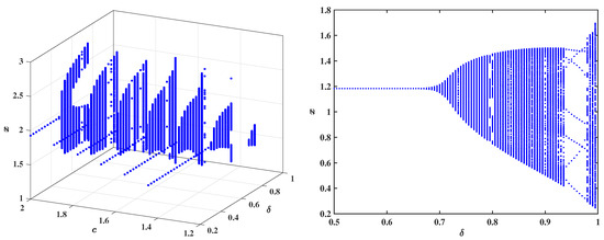
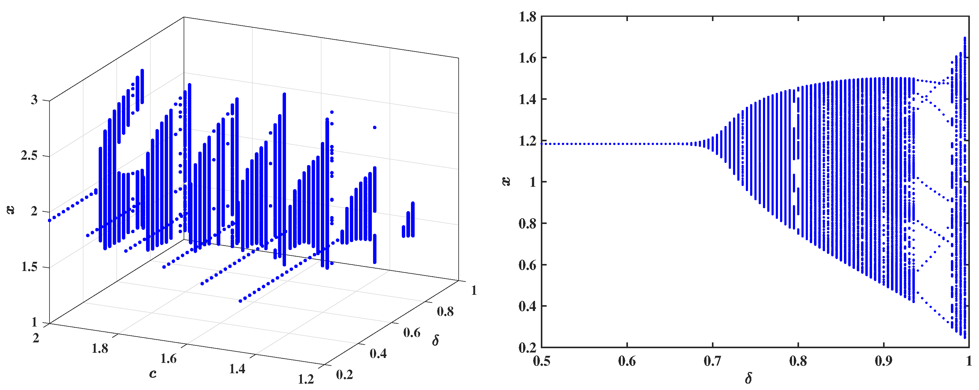
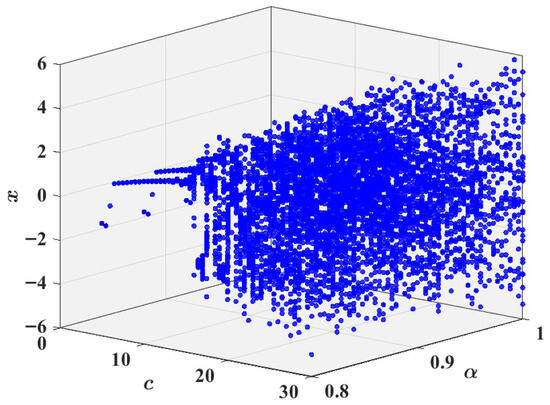
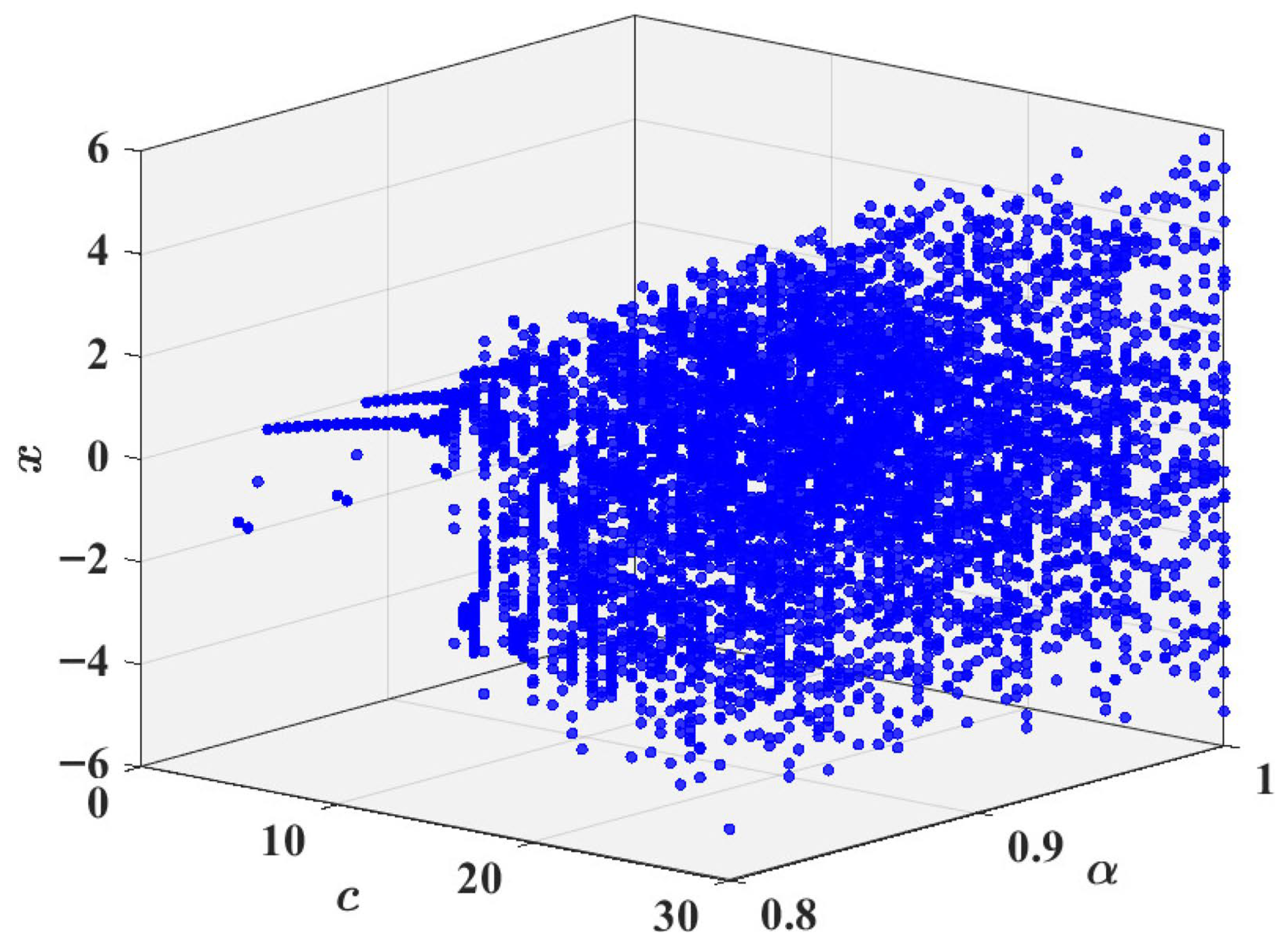
We now turn to the fractional-order T system. Figure 14 (left) shows the bifurcation diagram with respect to the fractional order $\alpha$ for $a=2,b=0.5,c=18$ and initial values near the equilibrium point. Consistent with the theoretical threshold ${\alpha }^{*}<0.9487$ obtained in Section 3, the system loses stability and transitions to chaos once $\alpha$ slightly exceeds this value. Figure 14 (right) plots the bifurcation diagram as a function of c with $a=2,b=0.5,\alpha =0.95$. The results indicate that the system becomes unstable as c approaches 18, which is consistent with the behavior observed in the left panel. A three-dimensional bifurcation structure in the $(\alpha ,c,x)$ space is further displayed in Figure 15, illustrating how variations in the fractional order reshape the dynamical landscape from stable equilibrium to unstable behavior.

Figure 14. (Left) Bifurcation diagram of the fractional T system (6) in $\alpha$-x plane with $a=2,b=0.5$ and $c=18$. (Right) Bifurcation diagram of the fractional T system (6) in c-x plane with $a=2,b=0.5$ and $\alpha =0.95$.

Figure 15. Three-dimensional bifurcation diagram of the fractional T system (6) as a function of $\alpha$ and c with $a=2,b=0.5$.

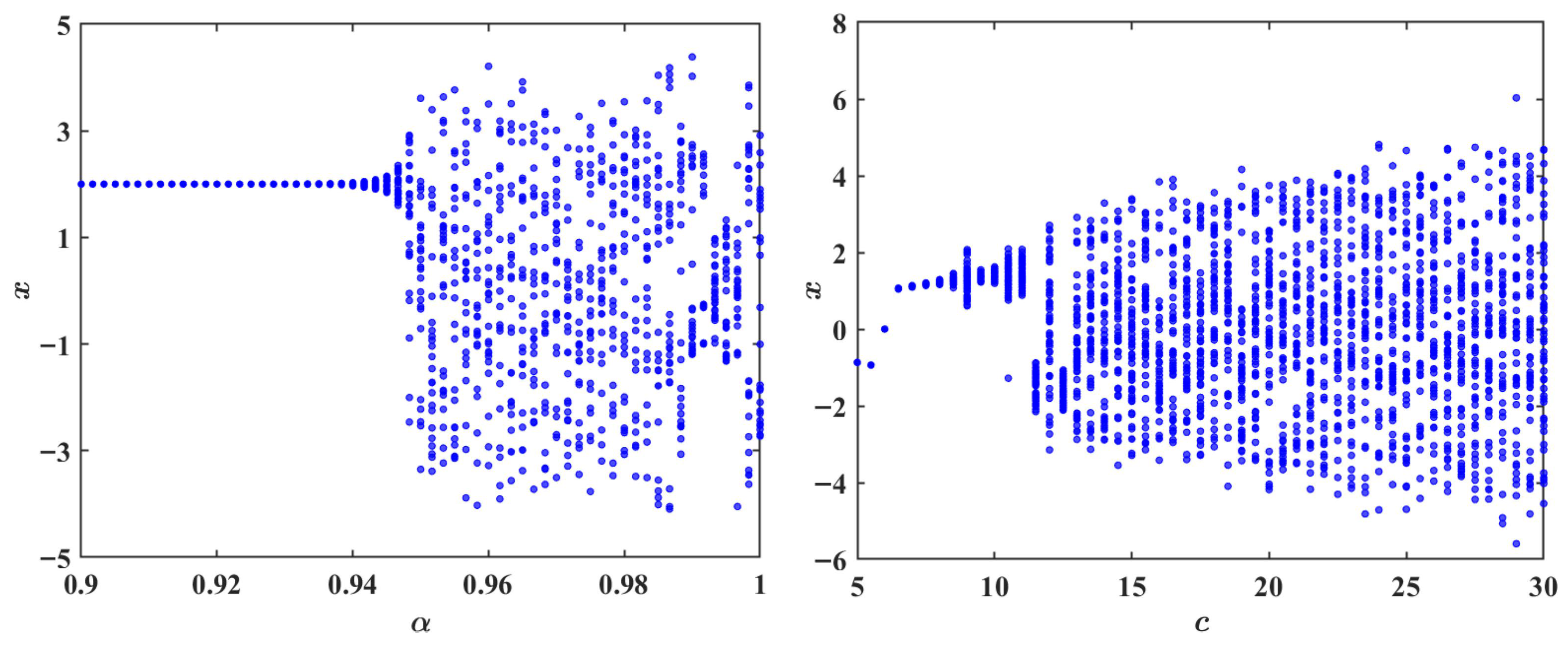
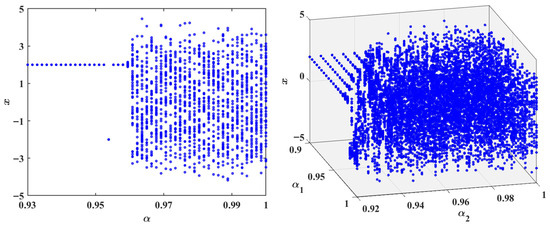
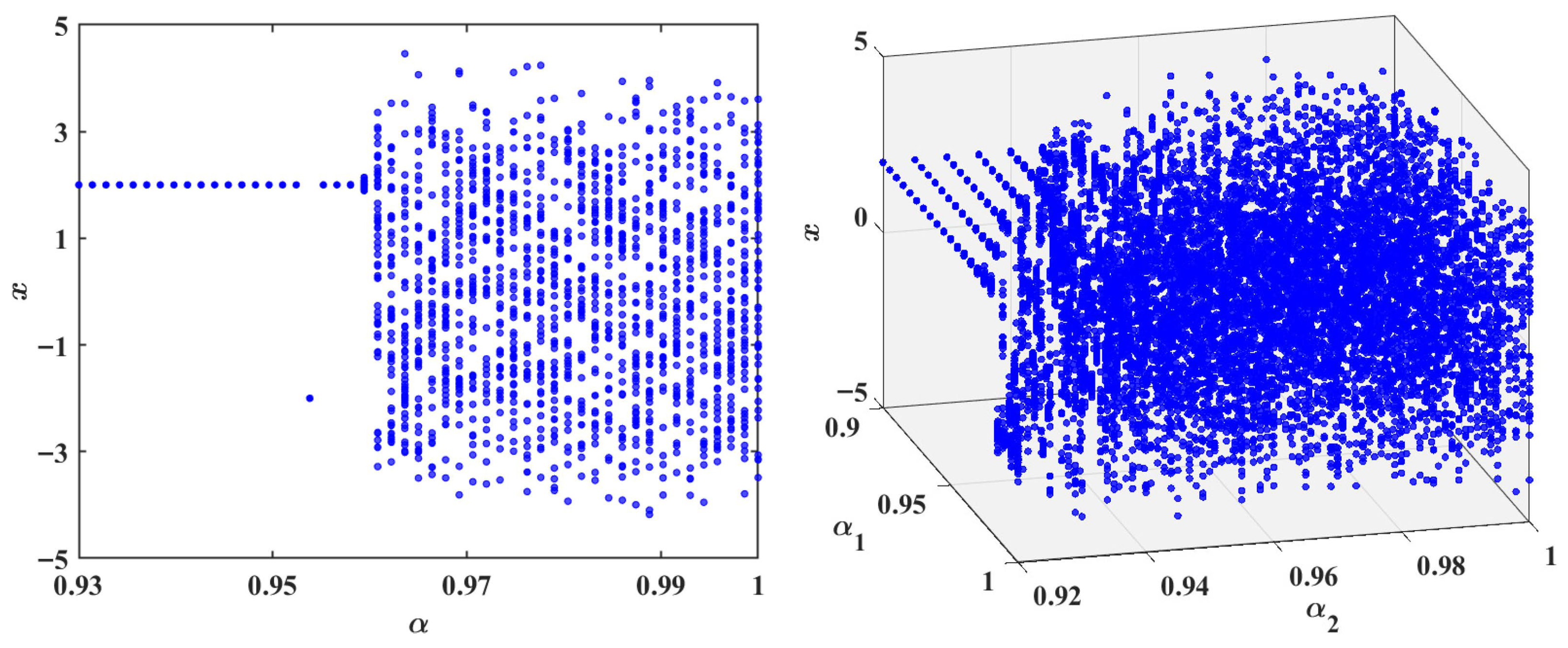
Additionally, we consider another parameter set $a=4$, $b=1$, $c=20$. The equilibria $E_1(2,2,4)$ and $E_2(-2,-2,4)$ possess eigenvalues $-5.55$, $0.276\pm 4.79i$. According to Theorem 1, the equilibria remain stable when ${\alpha }^{*}<0.964$. Since

$$r(Bcos\theta +Asin\theta )=659.9\ne 0,$$

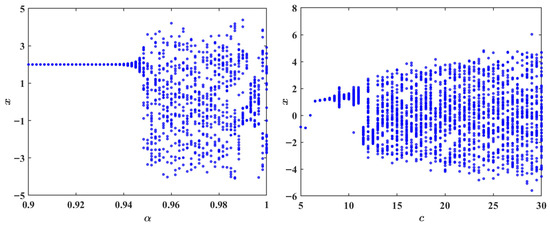
Theorem 2 implies that Hopf bifurcation occurs at $\alpha ={\alpha }^{*}$. The bifurcation diagram with respect to $\alpha$ is shown in Figure 16 (left), confirming stability for $\alpha <0.964$. Figure 16 (right) presents a two-parameter bifurcation diagram in the $({\alpha }_1,{\alpha }_2)$-plane for ${\alpha }_3=0.97$. The results show that, for each parameter ${\alpha }_i$, the system gradually transitions from a stable to an unstable state as the other fractional order varies.

Figure 16. (Left) Bifurcation diagram of the fractional T system (6) in $\alpha$-x plane under $a=4,b=1$ and $c=20$. (Right) Bifurcation diagram of the fractional T system (6) as a function of ${\alpha }_1$ and ${\alpha }_2$ with $a=4,b=1$ and $c=20$.

Taken together, these results indicate that fractional-order systems can exhibit more diverse dynamical behaviors than their integer-order counterparts. In particular, the fractional orders act as additional control parameters, allowing smooth transitions among stable, periodic, and chaotic regimes. This observation suggests that fractional-order formulations provide increased flexibility in modeling and regulating complex dynamical processes.

6. Conclusions

In this work, we developed a fast semi-implicit numerical scheme for the fractional-order T system. By combining a sum-of-exponentials approximation of the Caputo derivative with a carefully designed IMEX-type discretization, the resulting scheme is linear and decoupled at each time step, significantly improving computational efficiency and making it well suited for long-time simulations. A rigorous stability analysis of the proposed scheme was established.

Based on this framework, we numerically investigated the dynamical behaviors of the fractional-order T system. The numerical results, including Lyapunov exponents, time responses, phase portraits, and bifurcation diagrams, show that the fractional order plays an important role in shaping the system dynamics. In particular, variations in the fractional order influence stability regions, transient evolution, and bifurcation structures, demonstrating pronounced memory-induced effects on the qualitative behavior of the system. Similar phenomena have also been reported in other fractional-order chaotic systems, such as the Duffing system [40], Chua circuit [41], and Chen system [42].

The proposed numerical framework provides an efficient and reliable approach for long-time simulations of the fractional-order T system, significantly reducing the computational cost and memory requirements compared with classical methods. Future work may extend the present framework to more complex fractional systems, including coupled or higher-dimensional models, and investigate alternative fractional operators to further explore memory effects in nonlinear dynamical systems.

References

- Patnaik, S.; Semperlotti, F. Application of variable-and distributed-order fractional operators to the dynamic analysis of nonlinear oscillators. Nonlinear Dyn. 2020, 100, 561–580. [Google Scholar] [CrossRef] [Scilit]
- Matouk, A.E. Chaos, feedback control and synchronization of a fractional-order modified Autonomous Van der Pol–Duffing circuit. Commun. Nonlinear Sci. Numer. Simul. 2011, 16, 975–986. [Google Scholar] [CrossRef] [Scilit]
- Aghababa, M.P. Fractional modeling and control of a complex nonlinear energy supply-demand system. Complexity 2015, 20, 74–86. [Google Scholar] [CrossRef] [Scilit]
- Jajarmi, A.; Baleanu, D.; Vahid, K.Z.; Mobayen, S. A general fractional formulation and tracking control for immunogenic tumor dynamics. Math. Methods Appl. Sci. 2022, 45, 667–680. [Google Scholar] [CrossRef] [Scilit]
- Matouk, A.E. Chaotic attractors that exist only in fractional-order case. J. Adv. Res. 2023, 45, 183–192. [Google Scholar] [CrossRef] [Scilit]
- Almatroud, A.O. Extreme multistability of a fractional-order discrete-time neural network. Fractal Fract. 2021, 5, 202. [Google Scholar] [CrossRef] [Scilit]
- Liu, X.G.; Ma, L. Chaotic vibration, bifurcation, stabilization and synchronization control for fractional discrete-time systems. Appl. Math. Comput. 2020, 385, 125423. [Google Scholar] [CrossRef] [Scilit]
- Zhu, H.Y.; Yu, L.P. Dynamic behavior of the fractional-order ananthakrishna model for repeated yielding. Fractal Fract. 2025, 9, 425. [Google Scholar] [CrossRef] [Scilit]
- Lorenz, E.N. Deterministic non-periodic flows. J. Atmos. Sci. 1963, 20, 130–141. [Google Scholar] [CrossRef] [Scilit]
- Chen, G.; Ueta, T. Yet another chaotic attractor. Int. J. Bifurc. Chaos 1999, 9, 1465–1466. [Google Scholar] [CrossRef] [Scilit]
- Lü, J.H.; Chen, G.R. A new chaotic attractor coined. Int. J. Bifurc. Chaos 2002, 12, 659–661. [Google Scholar] [CrossRef] [Scilit]
- Qi, G.; Chen, G.; Du, C.; Chen, Z.; Yuan, Z. Analysis of a new chaotic system. Phys. A 2005, 352, 295–308. [Google Scholar]
- Liu, L.; Su, Y.; Liu, T. A modified Lorenz attractor. Int. J. Nonlinear Sci. 2006, 7, 187–191. [Google Scholar] [CrossRef] [Scilit]
- Sparrow, C. The Lorenz Equation: Bifurcations, Chaos and Strange Attractors; Springer: New York, NY, USA, 1982. [Google Scholar]
- Chen, G.; Dong, X. From Chaos to Order: Methodologies, Perspectives and Applications; World Scientific: Singapore, 1998. [Google Scholar]
- Tigan, G. Analysis of a dynamical system derived from the Lorenz system. Sci. Bull. Politeh. Univ. Timis. 2005, 50, 61–72. [Google Scholar]
- Tigan, G. Bifurcation and stability in a system derived from the Lorenz system. In Proceedings of the 3rd International Colloquium, Mathematics in Engineering and Numerical Physics, Bucharest, Romania, 7–9 October 2004; pp. 265–272. [Google Scholar]
- Jiang, B.; Hana, X.J.; Bi, Q.S. Hopf bifurcation analysis in the T system. Nonlinear Anal. Real. 2010, 11, 522–527. [Google Scholar] [CrossRef] [Scilit]
- Zeng, F.H.; Li, C.P.; Liu, F.W.; Turner, I. The use of finite difference/element approaches for solving the time-fractional subdiffusion equation. SIAM J. Sci. Comput. 2013, 35, A2976–A3000. [Google Scholar] [CrossRef] [Scilit]
- Lin, Y.M.; Li, X.J.; Xu, C.J. Finite difference/spectral approximations for the fractional cable equation. Math. Comput. 2011, 80, 1369–1396. [Google Scholar] [CrossRef] [Scilit]
- Gao, G.H.; Sun, Z.Z.; Zhang, H.W. A new fractional numerical differentiation formula to approximate the caputo fractional derivative and its applications. J. Comput. Phys. 2014, 259, 33–50. [Google Scholar] [CrossRef] [Scilit]
- Alikhanov, A.A. A new difference scheme for the time fractional diffusion equation. J. Comput. Phys. 2015, 280, 424–438. [Google Scholar] [CrossRef] [Scilit]
- Lv, C.W.; Xu, C.J. Error analysis of a high order method for time-fractional diffusion equation. SIAM J. Sci. Comput. 2016, 38, A2699–A2724. [Google Scholar] [CrossRef] [Scilit]
- Ford, N.J.; Yan, Y.B. An approach to construct higher order time discretisation schemes for time fractional partial differential equations with nonsmooth data. Fract. Calc. Appl. Anal. 2017, 20, 1076–1105. [Google Scholar] [CrossRef] [Scilit]
- Zeng, F.H.; Zhang, Z.Q.; Karniadakis, G.E. Second-order numerical methods for multi-term fractional differential equations: Smooth and non-smooth solutions. Comput. Methods Appl. Mech. Eng. 2017, 327, 478–502. [Google Scholar] [CrossRef] [Scilit]
- Baffet, D.; Hesthaven, J.S. High-order accurate adaptive kernel compression time-stepping schemes for fractional differential equations. J. Sci. Comput. 2017, 72, 1169–1195. [Google Scholar] [CrossRef] [Scilit]
- Baffet, D.; Hesthaven, J.S. A kernel compression scheme for fractional differential equations. SIAM J. Numer. Anal. 2017, 55, 496–520. [Google Scholar] [CrossRef] [Scilit]
- Jiang, S.D.; Zhang, J.W.; Zhang, Q.; Zhang, Z.M. Fast evaluation of the caputo fractional derivative and its applications to fractional diffusion equations. Commun. Comput. Phys. 2017, 21, 650–678. [Google Scholar] [CrossRef] [Scilit]
- Zhang, Q.; Zhang, J.W.; Jiang, S.D.; Zhang, Z.M. Numerical solution to a linearized time fractional KdV equation on unbounded domians. Math. Comp. 2018, 87, 693–719. [Google Scholar] [CrossRef] [Scilit]
- Zhang, H.; Zeng, F.H.; Jiang, X.Y.; Zhang, Z.M. Fast time-stepping discontinuous galerkin method for the subdiffusion equation. IMA J. Numer. Anal. 2024, 45, 3313–3341. [Google Scholar] [CrossRef]
- Zhu, H.Y.; Xu, C.J. A fast high order method for the time-fractional diffusion equation. SIAM J. Numer. Anal. 2019, 57, 2829–2849. [Google Scholar] [CrossRef] [Scilit]
- Podlubny, I. Fractional Differential Equations; Academic Press: New York, NY, USA, 1999. [Google Scholar]
- Diethelm, K. The Analysis of Fractional Differential Equations; Springer: Berlin/Heidelberg, Germany, 2010. [Google Scholar]
- Wang, J.; Liu, J.; Zhang, R. Stability and bifurcation analysis for a fractional-order cancer model with two delays. Chaos Solitons Fractals 2023, 173, 113732. [Google Scholar] [CrossRef] [Scilit]
- Beylkin, G.; Monzón, L. Approximation by exponential sums revisited. Appl. Comput. Harmon. Anal. 2010, 28, 131–149. [Google Scholar] [CrossRef] [Scilit]
- Liao, H.L.; Yan, Y.G.; Zhang, J.W. Unconditional convergence of a fast two-level linearized algorithm for semilinear subdiffusion equations. J. Sci. Comput. 2019, 80, 1–25. [Google Scholar] [CrossRef] [Scilit]
- Sun, Z.Z.; Gao, G.H. Fractional Differential Equations-Finite Difference Methods; Science Press: Beijing, China, 2021. [Google Scholar]
- Liao, H.L.; McLean, W.; Zhang, J.W. A discrete Gronwall inequality with applications to numerical schemes for subdiffusion problems. SIAM J. Numer. Anal. 2019, 57, 218–237. [Google Scholar] [CrossRef] [Scilit]
- Li, H.; Shen, Y.J.; Han, Y.J.; Dong, J.L.; Li, J. Determining lyapunov exponents of fractional-order systems: A general method based on memory principle. Chaos Solitons Fractals 2023, 168, 113167. [Google Scholar] [CrossRef] [Scilit]
- Arena, P.; Caponetto, R.; Fortuna, L.; Porto, D. Chaos in a fractional order Duffing system. In Proceedings of the ECCTD, Budapest, Hungary, 30 August–3 September 1997; pp. 1259–1262. [Google Scholar]
- Li, C.P.; Deng, W.H.; Xu, D. Chaos synchronization of the Chua system with a fractional order. Phys. A 2006, 360, 171–185. [Google Scholar] [CrossRef] [Scilit]
- Lu, J.G.; Chen, G.R. A note on the fractional-order Chen system. Chaos Solitons Fractals 2006, 27, 685–688. [Google Scholar] [CrossRef] [Scilit]
Disclaimer/Publisher’s Note: The statements, opinions and data contained in all publications are solely those of the individual author(s) and contributor(s) and not of MDPI and/or the editor(s). MDPI and/or the editor(s) disclaim responsibility for any injury to people or property resulting from any ideas, methods, instructions or products referred to in the content. |
© 2026 by the authors. Licensee MDPI, Basel, Switzerland. This article is an open access article distributed under the terms and conditions of the Creative Commons Attribution (CC BY) license.