Using the Natural Generalized Laplace Transform to Solve the Time-Fractional Navier–Stokes Equation

Abstract

This article proposes a novel approach for dealing with the time-fractional Navier–Stokes equations via the natural generalized Laplace transform decomposition method (NGLTDM). This hybrid method utilizes both the natural generalized Laplace transform (NGLT) and a decomposition method. The method is correct because the series solutions become more accurate when more terms are added. We establish precise theorems that verify the existence of solutions and the convergence of the series. The analysis shows that the suggested method is more general than the Homotopy Perturbation Method (HPM) and the Adomian Decomposition Method (ADM). Also, this approach can be applied to handle difficult fluid dynamics problems governed by the Navier–Stokes equations. This study enhances analytical methodologies for fractional-order flow models.

1. Introduction

The time-fractional Navier–Stokes equations are a big step forward in fluid dynamics, especially when it comes to modeling flow processes that are complicated and have memory effects and interactions that are not local. The were developed by adding fractional derivatives in time to the normal Navier–Stokes equations (NSE).

Researchers first developed the (NSE) in [1]. They are partial differential equations that explain how fluids that stay together move. It is very important to know that the Navier–Stokes equation is a basic tool for describing many physical phenomena in the field of fluid dynamics. These include fluid flow through pipes and atmospheric currents [2,3]. The Navier-Stokes equation (NSE) is a very useful tool for finding how viscous fluids and solid objects interact. It is the best tool in the fields of thermohydraulics, meteorology, petroleum engineering, plasma physics, and technology, as noted in [4]. Different researchers have employed various methodologies to obtain the solution to the NSE. For instance, the authors in [5] addressed the time-fractional Navier–Stokes equations utilizing an innovative analytical and approximate approach. In [6], the researchers solved the time-fractional NSE system using the hybrid method called the Laplace–Adomian decomposition method.

The Adomian decomposition transform method and the q-homotopy analysis transform method were used in [7] to get numerical results for the multi-dimensional NSE. The homotopy perturbation method, a new recursive transform method that uses natural transformation, was used to find the solution to the multi-dimensional NSE in [8]. In [9], the authors examine the solution of the multi-dimensional fractional NSE employing the Sumudu transform in conjunction with the Caputo fractional derivative.

The authors in [10] utilize the variational iteration transform method to deal with solutions of the fractional-order NSE. The generalized Laplace transform was first examined in [11], and further characteristics of this transformation were acquired in [12]; a Laplace-type integral transform associated with Adomian’s was utilized to derive the solution of nonlinear evolution equations featuring non-integer derivatives in [13]. In [14], the authors examined the solution of the fractional-order Kaup–Kupershmidt (KK) equation by employing the natural decomposition method, utilizing two distinct fractional derivatives: the Atangana–Baleanu derivative in Caputo form (ABC) and the Caputo–Fabrizio (CF) derivative.

The double generalized Laplace transform with the decomposition method was applied to gain the solution of nonlinear sine-Gordon and coupled sine-Gordon equations [15]; later the same technique was extended to solve a time-fractional partial differential equation [16]. In [17], the authors introduced the natural generalized Laplace transform decomposition method (NGLTDM) for obtaining analytical solutions to time-fractional linear and nonlinear dispersive dKdV-type equations. The author in [18] employed the natural generalized Laplace transform decomposition method (NGLTDM) to obtain the solution of the singular one-dimensional Boussinesq equation. Based on the aforementioned research, this article utilizes the new natural generalized Laplace transform (NGLT) and the double natural generalized Laplace transform (DNGLT) together with the decomposition method to investigate the solution of the time-fractional Navier–Stokes equation.

Observation: The abbreviations used in this study are as follows:

(1)

(GLT) as a replacement for ”Generalized Laplace Transform”.

(2)

(NT) as a replacement for ” Natural transform”.

(3)

(NGLT) as a replacement for ” natural generalized Laplace transform”.

(4)

(INGLT) as a replacement for ” inverse natural generalized Laplace transform”.

(5)

(NGLTDM) as a replacement for ” natural generalized Laplace transform decomposition method”.

(6)

(DNGLTDM) as a replacement for ” double natural generalized Laplace transform decomposition method”.

2. Important Ideas

This unit covers the most important definitions and properties of fractional calculus, as well as the single and DNGLT theory, which will be used throughout the article:

Definition 1 

([11]). Let $f\left(\sigma \right)$ be integrable, for $\forall \sigma \ge 0$. The generalized integral transform $G_{\upsilon }$ of the function $f\left(\sigma \right)$ is denoted by

$${\displaystyle F\left(s\right)=G_{\upsilon }\left(f\right)=s^{\upsilon }\underset{0}{\overset{\infty }{\int }}f\left(\sigma \right)e^{-\frac{\sigma }{s}}d\sigma ,}$$

(1)

for, $s\in \mathbb{C}$ and $\upsilon \in Z$.

Definition 2. 

The Caputo time-fractional derivative operator of order $\upsilon >0$ is determined by

$$D_{\sigma }^{\delta }\varphi (x_1,\sigma )=\left\{\begin{array}{c}{\displaystyle \frac{1}{\Gamma \left(m-\upsilon \right)}}{\int }_0^{\lambda }{\left(\sigma -\lambda \right)}^{m-\upsilon -1}{\displaystyle \frac{{\partial }^m\varphi (x_1,\tau )}{\partial {\sigma }^m}}d\tau ,\\ m-1<\delta <m,\\ {\displaystyle \frac{{\partial }^{m}u(x_1,\sigma )}{\partial {\sigma }^m}},\mathit{for}m=\delta \in \mathbb{N}\end{array}\right.,$$

For additional details, refer to [19].

The NGLT is defined as follows.

Definition 3 

([18]). Let $\varphi (x_1,\sigma )$ and $\varphi (x_1,x_2,\sigma )$ be functions of the definition of the (NGLT) of the functions $\varphi (x_1,\sigma )$ and $\varphi (x_1,x_2,\sigma )$; $x_1,x_2,\sigma \in {\mathbb{R}}^{+}$ are granted by

$${\displaystyle \Phi (p_1;u,s)=N_{x_1}^{+}{G}_{\upsilon }\left[\varphi \left(x_1,\sigma \right)\right]=\frac{s^{\upsilon }}{u}\underset{0}{\overset{\infty }{\int }}\underset{0}{\overset{\infty }{\int }}{e}^{-(\frac{p_1}{u}{x}_1+\frac{\sigma }{s})}\varphi \left(x_1,\sigma \right)d{x}_{1}d\sigma ,}$$

(2)

and the DNGLT is defined by

$$\begin{array}{ccc}\hfill \Phi (p_1;u,p_2;v,s)& =& N_{x_1,x_2}^{+}{G}_{\upsilon }\left[\varphi \left(x_1,x_2,\sigma \right)\right]\hfill \\ & =& {\displaystyle \frac{s^{\upsilon }}{uv}\underset{0}{\overset{\infty }{\int }}\underset{0}{\overset{\infty }{\int }}\underset{0}{\overset{\infty }{\int }}{e}^{-(\frac{p_1}{u}{x}_1+\frac{p_2}{v}{x}_2+\frac{\sigma }{s})}\varphi \left(x_1,x_2,\sigma \right)d{x}_1{x}_{2}d\sigma ,}\hfill \end{array}$$

(3)

where $N_{x_1}^{+}{G}_{\upsilon }$ and $N_2^{+}=N_{x_1,x_2}^{+}{G}_{\upsilon }$ indicate (NGLT) and (DNGLT) respectively and the symbols $p_1;u,p_2;v$ and s denote transforms of the variable $x_1,x_2$ and σ respectively.

Therefore, the inverse (NGLT) and (DNGLT) can be written, respectively, as

$$N_{p_1}^{-1}{G}_s^{-1}\left(\Phi (p_1;u,s)\right)=\varphi \left(x_1,\sigma \right)={\displaystyle \frac{1}{{\left(2\pi i\right)}^2}}{\int }_{\vartheta -i\infty }^{\vartheta +i\infty }{\int }_{\varrho -i\infty }^{\varrho -i\infty }{e}^{{\displaystyle \frac{p_1}{u}}{x}_1+{\displaystyle \frac{\sigma }{s}}}{N}_{x_1}^{+}{G}_{\upsilon }\left[\varphi \left(x_1,\sigma \right)\right]dsd{p}_1,$$

and

$$\begin{array}{cc}\hfill & \varphi \left(x_1,x_2,\sigma \right)\hfill \\ \hfill =& {\displaystyle \frac{1}{{\left(2\pi i\right)}^3}}{\int }_{\vartheta -i\infty }^{\vartheta +i\infty }{\int }_{\theta -i\infty }^{\theta +i\infty }{\int }_{\varrho -i\infty }^{\varrho -i\infty }{e}^{{\displaystyle \frac{p_1}{u}}{x}_1+{\displaystyle \frac{p_2}{v}}{x}_2+{\displaystyle \frac{\sigma }{s}}}{N}_2^{+}{G}_{\upsilon }\left[\varphi \left(x_1,x_2,\sigma \right)\right]dsd{p}_{2}d{p}_1,\hfill \end{array}$$

(4)

where the symbols $N_{p_{1;u}}^{-1}{G}_s^{-1}=N_1^{-1}{G}_s^{-1}$ and $N_2^{-1}{G}_s^{-1}=N_{p_1;u,p_{2;}v}^{-1}{G}_s^{-1}$ represent the inverse (NGLT) and (DNGLT) respectively.

Based on the definition of the natural generalized Laplace transform, we can derive the following transformation:

1.

Setting $\alpha =-1$, $p_1=1,s=v$, we obtain the double Sumudu transform:

$${\mathbf{S}}_{x_1}{S}_{\mathbf{\sigma }}\left[f(x_1,\mathbf{\sigma })\right]=F(u,v,)={\displaystyle \frac{1}{uv}}{\int }_0^{\infty }{\int }_0^{\infty }{e}^{-{\displaystyle \frac{1}{u}}{x}_1-{\displaystyle \frac{1}{v}}\mathbf{\sigma }}f(x_1,\mathbf{\sigma })d\mathbf{\sigma }d{x}_1.$$

2.

Setting $\alpha =0$, $u=1$ and $s={\displaystyle \frac{1}{s}}$, we obtain the double Laplace transform:

$$L_{x_1}{L}_{\mathbf{\sigma }}\left[f(x_1,\mathbf{\sigma })\right]=F(p_1,s)={\int }_0^{\infty }{\int }_0^{\infty }{e}^{-p_1{x}_1-s\mathbf{\sigma }}f(x_1,\mathbf{\sigma })d\mathbf{\sigma }d{x}_1.$$

3.

Setting $\alpha =0$, $u=1$, and $s=\omega$, we obtain the Laplace–Yang transform:

$$L_{x_1}Y\left[f(x_1,\mathbf{\sigma })\right]=F(p_1,\omega )={\int }_0^{\infty }{\int }_0^{\infty }{e}^{-p_1{x}_1-{\displaystyle \frac{1}{\omega }}\mathbf{\sigma }}f(x_1,\mathbf{\sigma })d\mathbf{\sigma }d{x}_1.$$

From the above remark, we conceded that the natural generalized Laplace transform is more general than other transformations.

The NGLT and DNGLT of the function $\varphi \left(x_1,\sigma \right)$ and $\varphi \left(x_1,x_2,\sigma \right)$ are proposed by $N_{x_1}^{+}{G}_{\upsilon }\left[\varphi \left(x_1,\sigma \right)\right]=\Phi (p_1;u,s)$ and $N_{x_1,x_2}^{+}{G}_{\upsilon }\left[\varphi \left(x_1,x_2,\sigma \right)\right]=\Phi (p_1;u,p_2;v,s)$ so, the NGLT and DNGLT of the partial derivatives ${\displaystyle \frac{\partial f(x_1,x_2,\sigma )}{\partial x_1}},{\displaystyle \frac{\partial f(x_1,x_2,\sigma )}{\partial \sigma }}$ and ${\displaystyle \frac{\partial f(x_1,x_2,\sigma )}{\partial x_2}}$ are presented by

$$\begin{array}{ccc}\hfill N_2^{+}{G}_{\upsilon }\left[{\displaystyle \frac{\partial \varphi (x_1,x_2,\sigma )}{\partial x_1}}\right]& =& {\displaystyle \frac{p_1\Phi F(p_1;u,p_2;v,s)}{u}}-{\displaystyle \frac{1}{u}}{N}_{x_2}^{+}{G}_{\upsilon }\left(\varphi \left(0,x_2,\sigma \right)\right),\hfill \\ \hfill N_2^{+}{G}_{\upsilon }\left[{\displaystyle \frac{\partial \varphi (x_1,x_2,\sigma )}{\partial x_2}}\right]& =& {\displaystyle \frac{p_2\Phi (p_1;u,p_2;v,s)}{v}}-{\displaystyle \frac{1}{v}}{N}_{x_1}^{+}{G}_{\upsilon }\left(\varphi \left(x_1,0,\sigma \right)\right),\hfill \\ \hfill N_2^{+}{G}_{\upsilon }\left[{\displaystyle \frac{\partial \varphi (x_1,x_2,\sigma )}{\partial \sigma }}\right]& =& {\displaystyle \frac{\Phi (p_1;u,p_2;v,s)}{s}}-s^{\upsilon }{N}_2^{+}\left(\varphi \left(x_1,x_2,0\right)\right).\hfill \end{array}$$

and $D_{\sigma }^{\delta }\varphi \left(x_1,\sigma \right)$ and $D_{\sigma }^{\delta }\left(x_1,x_2,\sigma \right)$ are provided by

$$\begin{array}{ccc}\hfill N_{x_1}^{+}{G}_{\upsilon }\left[D_{\sigma }^{\delta }\varphi \left(x_1,\sigma \right)\right]& =& {\displaystyle \frac{\Phi (p_1;u,s)}{s^{\delta }}}-s^{\upsilon -\delta +1}{N}_{x_1}^{+}\left[\varphi \left(x,0\right)\right],0<\delta \le 1\hfill \\ \hfill N_2^{+}{G}_{\upsilon }\left[D_{\sigma }^{\delta }\left(x_1,x_2,\sigma \right)\right]& =& {\displaystyle \frac{\Phi (p_1;u,p_2;v,s)}{s^{\delta }}}-s^{\upsilon -\delta +1}{N}_2^{+}\left[\varphi \left(x_1,x_2,0\right)\right],\hfill \end{array}$$

(5)

$$\begin{array}{c}\hfill 0<\delta \le 1.\end{array}$$

(6)

For further details, the reader is referred to [17]. The example below provides valuable support for the present analysis.

Example 1. 

The NGLT of the function $f(x_1,\sigma )=e^{i\left(a{x}_1+b\sigma \right)}$ is given by

$$N_x^{+}{G}_{\upsilon }\left[cos(a{x}_1+b\sigma )\right]={\displaystyle \frac{s^{\upsilon +1}\left(p_1-abus\right)}{\left(p_1^2+a^2{u}^2\right)\left(1+b^2{s}^2\right)}},$$

and

$$N_{x_1}^{+}{G}_{\upsilon }\left[sin(a{x}_1+b\sigma )\right]={\displaystyle \frac{s^{\upsilon +1}\left(au+bps\right)}{\left(p_1^2+a^2{u}^2\right)\left(1+b^2{s}^2\right)}}.$$

The following theorem is used to handle the singularities.

Theorem 1. 

The NGLT of the fractional partial derivatives $D_{\sigma }^{\delta }\varphi$ is denoted by

$$\begin{array}{ccc}\hfill N_{x_1}^{+}{G}_{\upsilon }\left[x_1{D}_{\sigma }^{\delta }\varphi \right]& =& {\displaystyle \frac{u}{s^{\delta }{p}_1}}{\displaystyle \frac{d}{du}}\left(u\Phi (p_1;u,s)\right)\hfill \\ & & -{\displaystyle \frac{u}{p_1}}{s}^{\upsilon -\delta +1}{\displaystyle \frac{d}{du}}\left(u\Phi (p_1;u,0)\right),\hfill \end{array}$$

(7)

$$N_{x_1}^{+}{G}_{\upsilon }\left[x_1{D}_{\sigma }^{\delta }\varphi \right]=-u{\displaystyle \frac{d}{d{p}_1}}{N}_{x_1}^{+}{G}_{\upsilon }\left[D_{\sigma }^{\delta }\varphi \right]$$

(8)

Proof. 

By utilizing the definition of NGLT, we have

$$N_{x_1}^{+}{G}_{\upsilon }\left[D_{\sigma }^{\delta }\varphi \right]={\int }_0^{\infty }{\int }_0^{\infty }{\displaystyle \frac{s^{\upsilon }}{u}}{e}^{-\left({\displaystyle \frac{p_1}{u}}{x}_1+{\displaystyle \frac{1}{s}}\sigma \right)}{D}_{\sigma }^{\delta }\varphi d{x}_{1}d\sigma ,$$

(9)

By utilizing the derivatives with respect to $u$ for Equation (9), we get

$$\begin{array}{cc}\hfill {\displaystyle \frac{d}{du}}{N}_{x_1}^{+}{G}_{\upsilon }\left[D_{\sigma }^{\delta }\varphi \right]& ={\displaystyle \frac{d}{du}}{\int }_0^{\infty }{\int }_0^{\infty }{\displaystyle \frac{s^{\upsilon }}{u}}{e}^{-\left({\displaystyle \frac{p_1}{u}}{x}_1+{\displaystyle \frac{1}{s}}\sigma \right)}{D}_{\sigma }^{\delta }\varphi d{x}_{1}d\sigma ,\hfill \\ \hfill & ={\int }_0^{\infty }{s}^{\upsilon }{e}^{-{\displaystyle \frac{1}{s}}\sigma }\left({\int }_0^{\infty }{\displaystyle \frac{d}{du}}{\displaystyle \frac{1}{u}}{e}^{-{\displaystyle \frac{p_1}{u}}{x}_1}{D}_{\sigma }^{\delta }\varphi d{x}_1\right)d\sigma ,\hfill \end{array}$$

(10)

you can find the derivative inside the brackets like this:

$$\begin{array}{ccc}\hfill {\int }_0^{\infty }{\displaystyle \frac{d}{du}}{\displaystyle \frac{1}{u}}{e}^{-{\displaystyle \frac{p_1}{u}}{x}_1}{D}_{\sigma }^{\delta }\varphi d{x}_1& =& {\int }_0^{\infty }\left({\displaystyle \frac{p_1}{u^3}}{x}_1-{\displaystyle \frac{1}{u^2}}\right)e^{-{\displaystyle \frac{p_1}{u}}{x}_1}{D}_{\sigma }^{\delta }\varphi d{x}_1\hfill \\ & =& {\int }_0^{\infty }{\displaystyle \frac{p_1}{u^3}}{x}_1{e}^{-{\displaystyle \frac{p_1}{u}}{x}_1}{D}_{\sigma }^{\delta }\varphi d{x}_1\hfill \\ & & -{\int }_0^{\infty }{\displaystyle \frac{1}{u^2}}{e}^{-{\displaystyle \frac{p_1}{u}}{x}_1}{D}_{\sigma }^{\delta }\varphi d{x}_1,\hfill \end{array}$$

(11)

By putting the right-hand-side of Equation (11) into Equation (10), we get

$$\begin{array}{cc}\hfill {\displaystyle \frac{d}{du}}\left(N_{x_1}^{+}{G}_{\upsilon }\left[D_{\sigma }^{\delta }\varphi \right]\right)=& {\int }_0^{\infty }{s}^{\upsilon }{e}^{-{\displaystyle \frac{1}{s}}\sigma }{\int }_0^{\infty }{\displaystyle \frac{p_1}{u^3}}{x}_1{e}^{-{\displaystyle \frac{p_1}{u}}{x}_1}{D}_{\sigma }^{\delta }\varphi d{x}_1\hfill \\ \hfill & -{\int }_0^{\infty }{s}^{\upsilon }{e}^{-{\displaystyle \frac{1}{s}}\sigma }{\int }_0^{\infty }{\displaystyle \frac{1}{u^2}}{e}^{-{\displaystyle \frac{p_1}{u}}{x}_1}{D}_{\sigma }^{\delta }\varphi d{x}_1,\hfill \end{array}$$

(12)

By arranging Equation (12), we have

$$\begin{array}{cc}\hfill {\displaystyle \frac{d}{du}}\left(N_{x_1}^{+}{G}_{\upsilon }\left[D_{\sigma }^{\delta }\varphi \right]\right)=& {\displaystyle \frac{p_1}{u^2}}\left({\displaystyle \frac{s^{\upsilon }}{u}}{\int }_0^{\infty }{\int }_0^{\infty }{e}^{-\left({\displaystyle \frac{p_1}{u}}{x}_1+{\displaystyle \frac{1}{s}}\sigma \right)}{x}_1{D}_{\sigma }^{\delta }\varphi d{x}_{1}d\sigma \right)\hfill \\ \hfill & -{\displaystyle \frac{1}{u}}\left({\displaystyle \frac{s^{\upsilon }}{u}}{\int }_0^{\infty }{\int }_0^{\infty }{e}^{-\left({\displaystyle \frac{p_1}{u}}{x}_1+{\displaystyle \frac{1}{s}}\sigma \right)}{D}_{\sigma }^{\delta }\varphi d{x}_{1}d\sigma \right),\hfill \end{array}$$

(13)

The first integral on the right side of Equation (13) is the NGLT of the function $x_1{D}_{\sigma }^{\delta }\varphi$ and the second integral is the NGLT of $D_{\sigma }^{\delta }\varphi$

$$\begin{array}{cc}\hfill {\displaystyle \frac{d}{du}}\left(N_{x_1}^{+}{G}_{\upsilon }\left[D_{\sigma }^{\delta }\varphi \right]\right)& ={\displaystyle \frac{p_1}{u^2}}{N}_{x_1}^{+}{G}_{\upsilon }\left[x_1{D}_{\sigma }^{\delta }\varphi \right]-{\displaystyle \frac{1}{u}}{N}_{x_1}^{+}{G}_{\upsilon }\left[D_{\sigma }^{\delta }\varphi \right],\hfill \end{array}$$

(14)

By manipulating Equation (14) and using Equation (5), we will obtain the proof for Equation (7) as follows

$$\begin{array}{ccc}\hfill N_{x_1}^{+}{G}_{\upsilon }\left[x_1{D}_{\sigma }^{\delta }\varphi \right]& =& {\displaystyle \frac{u}{s^{\delta }{p}_1}}{\displaystyle \frac{d}{du}}\left(u\Phi (p_1;u,s)\right)\hfill \\ & & -{\displaystyle \frac{u}{p_1}}{s}^{\upsilon -\delta +1}{\displaystyle \frac{d}{d{u}_1}}\left(u\Phi (p_1;u,0)\right),\hfill \end{array}$$

To establish Equation (9), we can use the derivatives concerning $p_1$, so we have

$$\begin{array}{ccc}\hfill {\displaystyle \frac{d}{d{p}_1}}{N}_{x_1}^{+}{G}_{\upsilon }\left[D_{\sigma }^{\delta }\varphi \right]& =& {\int }_0^{\infty }{\int }_0^{\infty }{\displaystyle \frac{s^{\upsilon }}{u}}{\displaystyle \frac{d}{d{p}_1}}{e}^{-\left({\displaystyle \frac{p_1}{u}}{x}_1+{\displaystyle \frac{1}{s}}\sigma \right)}{D}_{\sigma }^{\delta }\varphi d{x}_{1}d\sigma ,\hfill \\ & =& {\int }_0^{\infty }{\int }_0^{\infty }{\displaystyle \frac{-s^{\upsilon }}{u^2}}{e}^{-\left({\displaystyle \frac{p_1}{u}}{x}_1+{\displaystyle \frac{1}{s}}\sigma \right)}{x}_1{D}_{\sigma }^{\delta }\varphi d{x}_{1}d\sigma ,\hfill \end{array}$$

(15)

Hence, Equation (15) becomes

$$\begin{array}{ccc}\hfill {\displaystyle \frac{d}{d{p}_1}}{N}_{x_1}^{+}{G}_{\upsilon }\left[D_{\sigma }^{\delta }\varphi \right]& =& -{\displaystyle \frac{1}{u}}\left[{\displaystyle \frac{s^{\upsilon }}{u}}{\int }_0^{\infty }{\int }_0^{\infty }{e}^{-\left({\displaystyle \frac{p_1}{u}}{x}_1+{\displaystyle \frac{1}{s}}\sigma \right)}{x}_1{D}_{\sigma }^{\delta }\varphi d{x}_{1}d\sigma \right]\hfill \\ & =& -{\displaystyle \frac{1}{u}}{N}_{x_1}^{+}{G}_{\upsilon }\left[x_1{D}_{\sigma }^{\delta }\varphi \right],\hfill \end{array}$$

(16)

Therefore

$$N_{x_1}^{+}{G}_{\upsilon }\left[x_1{D}_{\sigma }^{\delta }\varphi \right]=-u{\displaystyle \frac{d}{d{p}_1}}{N}_{x_1}^{+}{G}_{\upsilon }\left[D_{\sigma }^{\delta }\varphi \right].$$

The proof is complete. □

3. Convergence Analysis and NGLTDM

This section of the article describes the foundational principles of the natural generalized Laplace transform decomposition method (NGLTDM), which is used to solve time-fractional partial differential equations.

Let us examine the following linear one-dimensional time-fractional partial differential equation along with its initial conditions condition:

$$D_{\sigma }^{\delta }\varphi +L\varphi \left(x_1,\sigma \right)+H\left(\varphi \left(x_1,\sigma \right)\right)=f(x_1,\sigma ),\sigma >0,0<\delta \le 1$$

(17)

and

$$\varphi (x_1,0)=f_1\left(x_1\right)$$

(18)

Here $D_{\sigma }^{\delta }$ denotes the Caputo fractional operator, L the linear differential operator, H the general nonlinear differential operator, and $f\left(x_1,\sigma \right)$ the external source term. To study the solution of Equation (17), we proceed through the following analytical steps:

Step 1: 

Applying the (NGLT) yields the following form of Equation (17).

$$N_{x_1}^{+}{G}_{\upsilon }\left[D_{\sigma }^{\delta }\varphi \right]+N_{x_1}^{+}{G}_{\upsilon }\left[L\varphi \left(x_1,\sigma \right)+H\left(\varphi \left(x_1,\sigma \right)\right)\right]=N_{x_1}^{+}{G}_{\upsilon }\left[f(x_1,\sigma )\right]$$

(19)

Step 2: 

Employing Equation (5), we get

$${\displaystyle \frac{\Phi (p_1;u,s)}{s^{\delta }}}-s^{\upsilon -\delta +1}{N}_{x_1}^{+}\left[\varphi \left(x_1,0\right)\right]=-N_{x_1}^{+}{G}_{\upsilon }\left[L\varphi \left(x_1,\sigma \right)+H\left(\varphi \left(x_1,\sigma \right)\right)\right]+F\left(p;u,s\right)$$

(20)

where $N_{x_1}^{+}\left[\varphi \left(x_1,0\right)\right]=F_1\left(p_1;u\right)$ and $N_{x_1}^{+}{G}_{\upsilon }\left[f(x_1,\sigma )\right]=F\left(p_1;u,s\right)$ are the NT and NGLT for $f_1\left(x_1,0\right)$ and $f\left(x_1,\sigma \right)$ respectively.

Step 3: 

Multiplying Equation (20) by $s^{\delta }$, one can get

$$\Phi (p_1;u,s)=s^{\upsilon +1}{F}_1\left(p_1;u\right)-s^{\delta }{N}_{x_1}^{+}{G}_{\upsilon }\left[L\varphi \left(x_1,\sigma \right)+H\left(\varphi \left(x_1,\sigma \right)\right)\right]+s^{\delta }F\left(p_1;u,s\right)$$

(21)

Step 4: 

Applying the inverse natural generalized Laplace transform to Equation (21)

$$\begin{array}{ccc}\hfill \varphi \left(x_1,\sigma \right)& =& f_1\left(x_1\right)+N_{p,u}^{-1}{G}_s^{-1}\left[s^{\delta }F\left(p_1;u,s\right)\right]\hfill \\ & & -N_{p,u}^{-1}{G}_s^{-1}\left[s^{\delta }{N}_{x_1}^{+}{G}_{\upsilon }\left[L\varphi \left(x_1,\sigma \right)+H\varphi \left(x_1,\sigma \right)\right]\right]\hfill \end{array}$$

(22)

Step 5: 

For the linear component, the following formulation is employed:

$$\varphi \left(x_1,\sigma \right)=\sum _{n=0}^{\infty }{\varphi }_n\left(x_1,\sigma \right).$$

(23)

For the nonlinear component, the formulation is expressed as follows:

$$H\varphi \left(x_1,\sigma \right)=\sum _{n=0}^{\infty }{\phi }_n\left(x_1,\sigma \right),$$

(24)

where ${\phi }_n\left(x_1,\sigma \right)$ is given by

$${\phi }_n\left(x_1,\sigma \right)={\displaystyle \frac{1}{n!}}{\displaystyle \frac{d^n}{d{\mu }^n}}\left[H\left(\sum _{k=0}^n{\mu }^k{\varphi }_n\left(x_1,\sigma \right)\right)\right],$$

(25)

Putting Equations (23) and (24) into Equation (22), is granted by

$$\begin{array}{ccc}\hfill \sum _{n=0}^{\infty }{\varphi }_n& =& f_1\left(x_1\right)+N_{p_1,u}^{-1}{G}_s^{-1}\left[s^{\delta }F\left(p_1;u,s\right)\right]\hfill \\ & & -N_{p_1,u}^{-1}{G}_s^{-1}\left[s^{\delta }{N}_{x_1}^{+}{G}_{\upsilon }\left[L\sum _{n=0}^{\infty }{\varphi }_n\left(x_1,\sigma \right)+\sum _{n=0}^{\infty }{\phi }_n\left(x_1,\sigma \right)\right]\right],\hfill \end{array}$$

(26)

where

$$\begin{array}{ccc}\hfill {\varphi }_0& =& f_1\left(x_1\right)+N_{p_1,u}^{-1}{G}_s^{-1}\left[s^{\delta }F\left(p_1;u,s\right)\right]\hfill \\ \hfill {\varphi }_1& =& -N_{p_1,u}^{-1}{G}_s^{-1}\left[s^{\delta }{N}_{x_1}^{+}{G}_{\upsilon }\left[L{\varphi }_0\left(x_1,\sigma \right)+N{\phi }_0\left(x_1,\sigma \right)\right]\right]\hfill \\ \hfill {\varphi }_2& =& -N_{p_1,u}^{-1}{G}_s^{-1}\left[s^{\delta }{N}_{x_1}^{+}{G}_{\upsilon }\left[L{\varphi }_1\left(x_1,\sigma \right)+N{\phi }_1\left(x_1,\sigma \right)\right]\right]\hfill \\ & & ·\hfill \\ & & ·\hfill \\ & & ·\hfill \\ \hfill {\varphi }_{n+1}& =& -N_{p_1,u}^{-1}{G}_s^{-1}\left[s^{\delta }{N}_{x_1}^{+}{G}_{\upsilon }\left[L{\varphi }_n\left(x_1,\sigma \right)+H{\varphi }_n\left(x_1,\sigma \right)\right]\right].\hfill \end{array}$$

(27)

The series solution of Equation (17) is given by Equation (23).

$$\varphi =\sum _{n=0}^{\infty }{\varphi }_n\left(x_1,\sigma \right)={\varphi }_0+{\varphi }_1+{\varphi }_2+\dots .$$

Theorem 2 (Uniqueness Theorem). 

Equation (17) has a unique solution, as long as $0<\rho <1$, where $\rho ={\displaystyle \frac{\left(l_1+l_2\right)}{\Gamma \left(\delta +1\right)}}{\sigma }^{\delta },$$\forall \sigma \in \left[0,T\right].$

Proof. 

Assume that $\left(\left[A\right],∥.∥\right)$ is the Banach space of all continuous functions defined on the $A=\left[0,T\right]$ and the norm $∥.∥$, then define $\Theta :A\to A$ in order that

$$\begin{array}{ccc}\hfill {\varphi }_{n+1}& =& f_1\left(x_1\right)+N_{p_1,u}^{-1}{G}_s^{-1}\left[s^{\delta }F\left(p_1;u,s\right)\right]\hfill \\ & & -N_{p_1,u}^{-1}{G}_s^{-1}\left[s^{\delta }{N}_{x_1}^{+}{G}_{\upsilon }\left[L\left({\varphi }_n\left(x_1,\sigma \right)\right)+H{\varphi }_n\left(x_1,\sigma \right)\right]\right],\hfill \end{array}$$

Presume that $L\left(\varphi \left(x_1,\sigma \right)\right)=\varphi \left(x_1,\sigma \right)$ and $H\varphi \left(x_1,\sigma \right)=W\varphi \left(x_1,\sigma \right),$ and additionally let

$$\left|W\left(\varphi \right)-W\left(\stackrel{\sim }{\varphi }\right)\right|<l_1\left|\varphi -\stackrel{\sim }{\varphi }\right|,$$

and

$$\left|L\left(\varphi \right)-L\left(\stackrel{\sim }{\varphi }\right)\right|<l_2\left|\varphi -\stackrel{\sim }{\varphi }\right|,$$

where $l_1,l_2$ are the Lipschitz constants with $0<l_1,l_2<1,$ and $\varphi ,\stackrel{\sim }{\varphi }$ are two various solutions of Equation (17). Hence

$$\begin{array}{ccc}\hfill ∥\Theta \left(\varphi \right)-\Theta \left(\stackrel{\sim }{\varphi }\right)∥& =& \underset{\sigma \in A}{max}\left|\begin{array}{c}{N}_{p_1,u}^{-1}{G}_s^{-1}\left[s^{\delta }{N}_{x_1}^{+}{G}_{\upsilon }\left[L\left(\varphi \right)+W\left(\varphi \right)\right]\right]\\ -N_{p_1,u}^{-1}{G}_s^{-1}\left[s^{\delta }{N}_{x_1}^{+}{G}_{\upsilon }\left[L\left(\stackrel{\sim }{\varphi }\right)+W\left(\stackrel{\sim }{\varphi }\right)\right]\right]\end{array}\right|,\hfill \\ & =& \underset{\sigma \in A}{max}\left|\begin{array}{c}{N}_{p_1,u}^{-1}{G}_s^{-1}\left[s^{\delta }{N}_{x_1}^{+}{G}_{\upsilon }\left[L\left(\varphi \right)-L\left(\stackrel{\sim }{\varphi }\right)\right]\right]\\ N_{p_1,u}^{-1}{G}_s^{-1}\left[s^{\delta }{N}_{x_1}^{+}{G}_{\upsilon }\left[W\left(\varphi \right)-W\left(\stackrel{\sim }{\varphi }\right)\right]\right]\end{array}\right|,\hfill \\ & \le & \underset{\sigma \in A}{max}\left(\begin{array}{c}\left|l_1{N}_{p_1,u}^{-1}{G}_s^{-1}\left[s^{\delta }{N}_{x_1}^{+}{G}_{\upsilon }\left[\left(\varphi -\stackrel{\sim }{\varphi }\right)\right]\right]\right|\\ +\left|l_2{N}_{p_1,u}^{-1}{G}_s^{-1}\left[s^{\delta }{N}_{x_1}^{+}{G}_{\upsilon }\left[\left(\varphi -\stackrel{\sim }{\varphi }\right)\right]\right]\right|\end{array}\right),\hfill \\ & \le & \underset{\sigma \in A}{max}\left(l_1+l_2\right)N_{p_1,u}^{-1}{G}_s^{-1}\left[s^{\delta }{N}_{x_1}^{+}{G}_{\upsilon }\left[1\right]\right]∥\left(\varphi -\stackrel{\sim }{\varphi }\right)∥,\hfill \end{array}$$

where

$$N_{p_1,u}^{-1}{G}_s^{-1}\left(s^{\delta }{N}_{x_1}^{+}{G}_{\upsilon }\left[1\right]\right)=N_{p_1,u}^{-1}{G}_s^{-1}\left({\displaystyle \frac{s^{\delta +\upsilon +1}}{p_1}}\right)={\displaystyle \frac{{\sigma }^{\delta }}{\Gamma \left(\delta +1\right)}},$$

Therefore, the above inequality becomes

$$\begin{array}{ccc}\hfill ∥\Theta \left(\varphi \right)-\Theta \left(\stackrel{\sim }{\varphi }\right)∥& \le & \left(l_1+l_2\right)N_{p_1,u}^{-1}{G}_s^{-1}\left[s^{\delta }{N}_{x_1}^{+}{G}_{\upsilon }\left[1\right]\right]∥\left(\varphi -\stackrel{\sim }{\varphi }\right)∥\hfill \\ & =& {\displaystyle \frac{\left(l_1+l_2\right){\sigma }^{\delta }}{\Gamma \left(\delta +1\right)}}∥\left(\varphi -\stackrel{\sim }{\varphi }\right)∥.\hfill \end{array}$$

So, according to the Banach fixed-point theorem for contractions in [20], there is a unique solution to Equation (17). Since ($0<\rho <1$), it follows that $\Theta$ is a contraction mapping. So, the proof is complete. □

Theorem 3 (Convergence Theorem). 

Let $\left(A,∥·∥\right)$ be a Banach space and $\Theta :A\to A$ be a mapping associated with NGLTMD defined by Equation (23). Consequently, Θ has a unique fixed point, and $0<\gamma <1;$ the series solution of Equation (23) converges to the solution in (17).

Proof. 

To show that ${\S }_i$ is a Cauchy sequence in $\left(\Delta ,∥·∥\right),$ let $\left\{{\S }_i\right\}$ denote the partial sum sequence corresponding to Equation (23). Assume that

$$\begin{array}{ccc}\hfill ∥{\S }_{i+1}-{\varphi }_i∥& =& ∥{\varphi }_{i+1}∥\le \gamma ∥{\varphi }_i\left(x_1,\sigma \right)∥\hfill \\ & \le & {\gamma }^2∥{\varphi }_{i-1}\left(x_1,\sigma \right)∥\le {\gamma }^3∥{\varphi }_{i-2}\left(x_1,\sigma \right)∥\hfill \\ \hfill \dots & \le & {\gamma }^{i+1}∥{\varphi }_0\left(x_1,\sigma \right)∥.\hfill \end{array}$$

Given a partial sum sequence ${\S }_i$ and ${\S }_j$, where $i,j\in \mathbb{N}$ and $i\ge j,$ utilizing the triangle inequality, it follows that

$$\begin{array}{ccc}\hfill ∥{\varphi }_i-{\varphi }_j∥& =& ∥{\varphi }_i-{\varphi }_{i-1}+{\varphi }_{i-1}-{\varphi }_{i-2}+\dots +{\varphi }_{j+2}-{\varphi }_{j+1}+{\varphi }_{j+1}-{\varphi }_j∥,\hfill \\ & \le & ∥{\varphi }_i-{\varphi }_{i-1}∥+∥{\varphi }_{i-1}-{\varphi }_{i-2}∥+\dots +∥{\varphi }_{j+2}-{\varphi }_{j+1}∥+∥{\varphi }_{j+1}-{\varphi }_j∥,\hfill \\ & \le & {\gamma }^i∥{\varphi }_0\left(x_1,\sigma \right)∥+{\gamma }^{i-1}∥{\varphi }_0\left(x_1,\sigma \right)∥+\dots \hfill \\ & & \dots +{\gamma }^{j+2}∥{\varphi }_0\left(x_1,\sigma \right)∥+{\gamma }^{j+1}∥{\varphi }_0\left(x_1,\sigma \right)∥\hfill \\ & \le & \left({\gamma }^i+{\gamma }^{i-1}+\dots +{\gamma }^{m+2}+{\gamma }^{j+1}\right)∥{\varphi }_0\left(x_1,\sigma \right)∥,\hfill \\ & =& {\gamma }^{j+1}\left({\gamma }^{i-j-1}+{\gamma }^{i-j-2}+\dots +1\right)∥{\varphi }_0\left(x_1,\sigma \right)∥,\hfill \\ & \le & {\gamma }^{j+1}\left({\displaystyle \frac{1-{\gamma }^{i-j}}{1-\gamma }}\right)∥{\varphi }_0\left(x_1,\sigma \right)∥,\hfill \end{array}$$

(28)

from $0<\gamma <1$ we notice that $1-{\gamma }^{i-j}\le 1$; thus

$$∥{\varphi }_i-{\varphi }_j∥\le {\displaystyle \frac{{\gamma }^{j+1}}{1-\gamma }}∥{\varphi }_0\left(x_1,\sigma \right)∥,$$

and since ${\varphi }_0\left(x_1,\sigma \right)$ is bounded, hence $∥{\varphi }_i-{\varphi }_j∥\to 0$ at $i,j\to \infty$. Hence, the sequence $\left\{{\varphi }_i\right\}$ is a Cauchy sequence

Consequently, the sequence in the Banach space is $\left(\Delta ,∥·∥\right)$. It follows that the series solution of Equation (23) converges, which completes the proof of the theorem. □

4. Analysis of the Natural Generalized Laplace Transform Decomposition Method (NGLTDM)

In this part of the paper, the NGLTDM is a mix of analytical methods that works well and is strong enough to solve fractional NSE.

In order to demonstrate the essential strategy of the NGLTDM, we consider the following time-fractional NSE

$$\begin{array}{ccc}\hfill D_{\sigma }^{\delta }\varphi (x_1,\sigma )& =& D_{x_1}^2\varphi (x_1,\sigma )+{\displaystyle \frac{1}{x_1}}{D}_{x_1}\varphi (x_1,\sigma )+f(x_1,\sigma ),x_1,\sigma >0,\hfill \\ \hfill m-1& <& \delta <m;\hfill \end{array}$$

(29)

under the initial condition

$$\varphi (x_1,0)=f_1\left(x_1\right)$$

where $D_{\sigma }^{\delta }={\displaystyle \frac{{\partial }^{\delta }}{\partial {\sigma }^{\delta }}}$ is the fractional Caputo derivative, $D_{x_1}^2={\displaystyle \frac{{\partial }^2}{\partial x_1^2}}$, $D_{x_1}={\displaystyle \frac{\partial }{\partial x_1}}$ and the right-hand-side function $f(x_1,\sigma )$ is the source term. To utilize the NGLTDM, the following steps are required:

Step 1: 

We multiply first Equation (29) by $x_1,$ and obtain

$$x_1{D}_{\sigma }^{\delta }\varphi =x_1{D}_{x_1}^2\varphi +D_{x1}\varphi +x_{1}f(x_1,\sigma ),x_1,\sigma >0.$$

(30)

Step 2: 

Applying the NGLT on both sides of Equation (2), we have

$$N_{x_1}^{+}{G}_{\upsilon }\left[x_1{D}_{\sigma }^{\delta }\varphi \right]=N_{x_1}^{+}{G}_{\upsilon }\left[x_1{D}_{x_1}^2\varphi +D_{x1}\varphi +x_{1}f(x_1,\sigma )\right],$$

(31)

By using Theorem 1, we get

$$\begin{array}{ccc}& & {\displaystyle \frac{u}{s^{\delta }{p}_1}}{\displaystyle \frac{d}{du}}\left(u\Phi (p_1;u,s)\right)-{\displaystyle \frac{u}{p_1}}{s}^{\upsilon -\delta +1}{\displaystyle \frac{d}{du}}\left(u\Phi (p_1;u,0)\right)\hfill \\ & =& N_{x_1}^{+}{G}_{\upsilon }\left[x_1{D}_{x_1}^2\varphi +D_{x1}\varphi +x_{1}f(x_1,\sigma )\right],\hfill \end{array}$$

After algebraic manipulation, we obtain

$$\begin{array}{ccc}\hfill {\displaystyle \frac{d}{du}}\left(u\Phi (p_1;u,s)\right)& =& s^{\upsilon +1}{\displaystyle \frac{d}{du}}\left(u\Phi (p_1;u,0)\right)\hfill \\ & & +{\displaystyle \frac{p_1{s}^{\delta }}{u}}{N}_{x_1}^{+}{G}_{\upsilon }\left[x_1{D}_{x_1}^2\varphi +D_{x1}\varphi +x_{1}f(x_1,\sigma )\right],\hfill \end{array}$$

(32)

Step 3: 

By taking the integral for both sides of Equation (32) from 0 to u with respect to u, we get

$$\begin{array}{ccc}\hfill \Phi (p_1;u,s)& =& s^{\upsilon +1}{F}_1(p_1;u,0)+{\displaystyle \frac{1}{u}}{\int }_0^u\left({\displaystyle \frac{p_1{s}^{\delta }}{u}}{N}_{x_1}^{+}{G}_{\upsilon }\left[x_{1}f(x_1,\sigma )\right]\right)du\hfill \\ & & +{\displaystyle \frac{1}{u}}{\int }_0^u\left({\displaystyle \frac{p_1{s}^{\delta }}{u}}{N}_{x_1}^{+}{G}_{\upsilon }\left[x_1{D}_{x_1}^2\varphi +D_{x1}\varphi \right]\right)du,\hfill \end{array}$$

(33)

Step 4: 

By employing the inverse NGLT for Equation (33), we get

$$\begin{array}{ccc}\hfill \varphi \left(x_1,\sigma \right)& =& f_1\left(x_1\right)+N_1^{-1}{G}_s^{-1}\left[{\displaystyle \frac{1}{u}}{\int }_0^u\left({\displaystyle \frac{p_1{s}^{\delta }}{u}}{N}_{x_1}^{+}{G}_{\upsilon }\left[x_1{D}_{x_1}^2\varphi +D_{x1}\varphi \right]\right)du\right]\hfill \\ & & +N_1^{-1}{G}_s^{-1}\left[{\displaystyle \frac{1}{u}}{\int }_0^u\left({\displaystyle \frac{p_1{s}^{\delta }}{u}}{N}_{x_1}^{+}{G}_{\upsilon }\left[x_{1}f(x_1,\sigma )\right]\right)du\right],\hfill \end{array}$$

(34)

where the symbol $N_u^{-1}{G}_s^{-1}$ indicates the inverse NGLT. The NGLTDM represents the solution as an infinite series as

$${\displaystyle \varphi \left(x_1,\sigma \right)=\sum _{m=0}^{\infty }{\varphi }_m\left(x_1,\sigma \right),}$$

(35)

by substituting Equation (35) into Equation (33), we get

$$\begin{array}{cc}\hfill {\displaystyle \sum _{m=0}^{\infty }{\varphi }_m\left(x_1,\sigma \right)}& =f\left(x_1\right)+N_1^{-1}{G}_s^{-1}\left[{\displaystyle \frac{1}{u}}{\int }_0^u\left({\displaystyle \frac{p_1{s}^{\delta }}{u}}{N}_{x_1}^{+}{G}_{\upsilon }\left[x_{1}f(x_1,\sigma )\right]\right)du\right]\hfill \\ \hfill & +N_1^{-1}{G}_s^{-1}\left[{\displaystyle \frac{1}{u}}{\int }_0^u\left({\displaystyle \frac{p_1{s}^{\delta }}{u}}{N}_{x_1}^{+}{G}_{\upsilon }\left[{\displaystyle \sum _{m=0}^{\infty }\left(x_1{D}_{x_1}^2{\varphi }_m+D_{x_1}{\varphi }_m\right)}\right]\right)du\right],\hfill \end{array}$$

(36)

by using NGLTDM, we introduce the recursive relations as:

$${\varphi }_0\left(x_1,\sigma \right)=f\left(x_1\right)+N_1^{-1}{G}_s^{-1}\left[{\displaystyle \frac{1}{u}}{\int }_0^u\left({\displaystyle \frac{p_1{s}^{\delta }}{u}}{N}_{x_1}^{+}{G}_{\upsilon }\left[x_{1}f(x_1,\sigma )\right]\right)du\right],$$

(37)

and the remainder of the terms can be obtained from the following formula

$${\varphi }_{m+1}\left(x_1,\sigma \right)=N_1^{-1}{G}_s^{-1}\left[{\displaystyle \frac{1}{u}}{\int }_0^u\left({\displaystyle \frac{p_1{s}^{\delta }}{u}}{N}_{x_1}^{+}{G}_{\upsilon }\left(x_1{D}_{x_1}^2{\varphi }_m+D_{x_1}{\varphi }_m\right)\right)d{u}_1\right],m\ge 1$$

(38)

5. Analysis of the Method of Double Natural Generalized Laplace Transform Decomposition Method (DNGLTDM)

The DNGLTDM is a powerful and adaptable approach for solving a wide range of fractional partial differential equations (FPDEs). It makes hard problems easier and offers exact series solutions for difficult cases. We discuss the following (2 + 1)-dimensional time-fractional NSE.

$$\begin{array}{ccc}\hfill D_{\sigma }^{\delta }\varphi +\varphi {\displaystyle \frac{\partial \varphi }{\partial x_1}}+\omega {\displaystyle \frac{\partial \varphi }{\partial x_2}}& =& \zeta \left({\displaystyle \frac{{\partial }^2\varphi }{\partial x_1^2}}+{\displaystyle \frac{{\partial }^2\varphi }{\partial x_2^2}}\right)+{\mu }_1,\hfill \\ \hfill D_{\sigma }^{\delta }\omega +\varphi {\displaystyle \frac{\partial \omega }{\partial x_1}}+\omega {\displaystyle \frac{\partial \omega }{\partial x_2}}& =& \zeta \left({\displaystyle \frac{{\partial }^2\omega }{\partial x_1^2}}+{\displaystyle \frac{{\partial }^2\omega }{\partial x_2^2}}\right)-{\mu }_2,\hfill \\ \hfill x_1,x_2,\sigma & >& 0,n-1<\delta <n;\hfill \end{array}$$

(39)

given the initial condition

$$\varphi (x_1,x_2,0)=f_1(x_1,x_2),\omega (x_1,x_2,0)=f_2(x_1,x_2)$$

(40)

where $D_{\sigma }^{\delta }={\displaystyle \frac{{\partial }^{\delta }}{\partial {\sigma }^{\delta }}}$ is the fractional Caputo derivative, k is defined as the kinematic viscosity of the flow. $\mu$ denotes dynamic viscosity and $\rho$ is density; ${\mu }_1=$${\displaystyle \frac{1}{\rho }}{\displaystyle \frac{\partial p}{\partial x_1}}$ and ${\mu }_2=-{\displaystyle \frac{1}{\rho }}{\displaystyle \frac{\partial p}{\partial x_2}}.$ To get a solution for Equation (39), the following next steps are necessary.

1.

By applying DNGLT for Equation (39), one can get

$$\begin{array}{ccc}\hfill {\displaystyle \frac{\Phi (p_1;u,p_2;v,s)}{s^{\delta }}}& =& s^{\upsilon -\delta +1}{N}_2^{+}\left(\varphi (x_1,x_2,0)\right)-N_2^{+}{G}_{\upsilon }\left(\varphi {\displaystyle \frac{\partial \varphi }{\partial x_1}}+\omega {\displaystyle \frac{\partial \varphi }{\partial x_2}}\right)\hfill \\ & & +N_2^{+}{G}_{\upsilon }\left(k\left({\displaystyle \frac{{\partial }^2\varphi }{\partial x_1}}+{\displaystyle \frac{{\partial }^2\varphi }{\partial x_2^2}}\right)\right)-N_2^{+}{G}_{\upsilon }\left({\mu }_1\right),\hfill \\ \hfill {\displaystyle \frac{\Psi (p_1;u,p_2;v,s)}{s^{\delta }}}& =& s^{\upsilon -\delta +1}{N}_2^{+}\left(\omega (x_1,x_2,0)\right)-N_2^{+}{G}_{\upsilon }\left(\varphi {\displaystyle \frac{\partial \omega }{\partial x_1}}+\omega {\displaystyle \frac{\partial \omega }{\partial x_2}}\right)\hfill \\ & & +N_2^{+}{G}_{\upsilon }\left(k\left({\displaystyle \frac{{\partial }^2\omega }{\partial x_1^2}}+{\displaystyle \frac{{\partial }^2\omega }{\partial x_2^2}}\right)\right)+N_2^{+}{G}_{\upsilon }\left({\mu }_2\right),\hfill \end{array}$$

(41)

2.

Now, taking DGLT for Equation (40) and substituting in Equation (41), we have

$$\begin{array}{ccc}\hfill \Phi (p_1;u,p_2;v,s)& =& s^{\upsilon +1}{F}_1\left(p_1;u,p_2;v\right)-s^{\delta }{N}_2^{+}{G}_{\upsilon }\left(\varphi {\displaystyle \frac{\partial \varphi }{\partial x_1}}+\omega {\displaystyle \frac{\partial \varphi }{\partial x_2}}\right)\hfill \\ & & +s^{\delta }{N}_2^{+}{G}_{\upsilon }\left(k\left({\displaystyle \frac{{\partial }^2\varphi }{\partial x_1}}+{\displaystyle \frac{{\partial }^2\varphi }{\partial x_2^2}}\right)\right)-s^{\delta }{N}_2^{+}{G}_{\upsilon }\left({\mu }_1\right),\hfill \\ \hfill \Psi (p_1;u,p_2;v,s)& =& s^{\upsilon +1}{F}_2\left(p_1;u,p_2;v\right)-s^{\delta }{N}_2^{+}{G}_{\upsilon }\left(\varphi {\displaystyle \frac{\partial \omega }{\partial x_1}}+\omega {\displaystyle \frac{\partial \omega }{\partial x_2}}\right)\hfill \\ & & +s^{\delta }{N}_2^{+}{G}_{\upsilon }\left(k\left({\displaystyle \frac{{\partial }^2\omega }{\partial x_1^2}}+{\displaystyle \frac{{\partial }^2\omega }{\partial x_2^2}}\right)\right)+s^{\delta }{N}_2^{+}{G}_{\upsilon }\left({\mu }_2\right),\hfill \end{array}$$

(42)

where $\Psi (p_1;u,p_2;v,s)$ is the DNGLT of $\omega (x_1,x_2,\sigma )$.

3.

On using inverse DNGLT for Equation (42), we get

$$\begin{array}{ccc}\hfill \varphi (x_1,x_2,\sigma )& =& N_2^{-1}{G}_s^{-1}\left(s^{\upsilon +1}{F}_1\left(p_1;u,p_2;v\right)-s^{\delta }{N}_2^{+}{G}_{\upsilon }\left({\mu }_1\right)\right)\hfill \\ & & -N_2^{-1}{G}_s^{-1}\left(s^{\delta }{N}_2^{+}{G}_{\upsilon }\left(\varphi {\displaystyle \frac{\partial \varphi }{\partial x_1}}+\omega {\displaystyle \frac{\partial \varphi }{\partial x_2}}\right)\right)\hfill \\ & & +N_2^{-1}{G}_s^{-1}\left(s^{\delta }{N}_2^{+}{G}_{\upsilon }\left(k\left({\displaystyle \frac{{\partial }^2\varphi }{\partial x_1^2}}+{\displaystyle \frac{{\partial }^2\varphi }{\partial x_2^2}}\right)\right)\right)\hfill \end{array}$$

(43)

and

$$\begin{array}{ccc}\hfill \omega (x_1,x_2,\sigma )& =& N_2^{-1}{G}_s^{-1}\left(s^{\upsilon +1}{F}_2\left(p_1;u,p_2;v\right)+s^{\delta }{N}_2^{+}{G}_{\upsilon }\left({\mu }_2\right)\right)\hfill \\ & & -N_2^{-1}{G}_s^{-1}\left(s^{\delta }{N}_2^{+}{G}_{\upsilon }\left(\varphi {\displaystyle \frac{\partial \omega }{\partial x_1}}+\omega {\displaystyle \frac{\partial \omega }{\partial x_2}}\right)\right)\hfill \\ & & +N_2^{-1}{G}_s^{-1}\left(s^{\delta }{N}_2^{+}{G}_{\upsilon }\left(k\left({\displaystyle \frac{{\partial }^2\omega }{\partial x_1^2}}+{\displaystyle \frac{{\partial }^2\omega }{\partial x_2^2}}\right)\right)\right).\hfill \end{array}$$

(44)

4.

The DNGLTDM solution $\varphi (x_1,x_2,\sigma )$ and $\omega (x_1,x_2,\sigma )$ are offered by the following infinite series

$$\begin{array}{ccc}\hfill \varphi (x_1,x_2,\sigma )& =& {\displaystyle \sum _{n=0}^{\infty }{\varphi }_n(x_1,x_2,\sigma ),}\hfill \\ \hfill \omega (x_1,x_2,\sigma )& =& {\displaystyle \sum _{n=0}^{\infty }{\omega }_n(x_1,x_2,\sigma ),}\hfill \end{array}$$

(45)

Therefore, the nonlinear terms $\varphi {\displaystyle \frac{\partial \varphi }{\partial x_1}},\omega {\displaystyle \frac{\partial \varphi }{\partial x_2}},\varphi {\displaystyle \frac{\partial \omega }{\partial x_1}}$ and $\omega {\displaystyle \frac{\partial \omega }{\partial x_2}}$ are fixed by

$$\begin{array}{ccc}\hfill \varphi {\displaystyle \frac{\partial \varphi }{\partial x_1}}& =& {\displaystyle \sum _{n=0}^{\infty }{A}_n,\omega \frac{\partial \varphi }{\partial x_2}=\sum _{n=0}^{\infty }{B}_n,}\hfill \\ \hfill \varphi {\displaystyle \frac{\partial \omega }{\partial x_1}}& =& {\displaystyle \sum _{n=0}^{\infty }{C}_n,\omega \frac{\partial \omega }{\partial x_2}=\sum _{n=0}^{\infty }{D}_n.}\hfill \end{array}$$

(46)

5.

By substituting Equations (45) and (46) into Equations (43) and (44), one can get

$$\begin{array}{ccc}\hfill {\displaystyle \sum _{n=0}^{\infty }{\varphi }_n(x_1,x_2,\sigma )}& =& N_2^{-1}{G}_s^{-1}\left(s^{\upsilon +1}{F}_1\left(p_1;u,p_2;v\right)-s^{\delta }{N}_2^{+}{G}_{\upsilon }\left({\mu }_1\right)\right)\hfill \\ & & -N_2^{-1}{G}_s^{-1}\left(s^{\delta }{N}_2^{+}{G}_{\upsilon }\left({\displaystyle \sum _{n=0}^{\infty }\left(A_n+B_n\right)}\right)\right)\hfill \\ & & +N_2^{-1}{G}_s^{-1}\left(s^{\delta }{N}_2^{+}{G}_{\upsilon }\left(k\left({\displaystyle \sum _{n=0}^{\infty }\left(\frac{{\partial }^2{\varphi }_n}{\partial x_1^2}+\frac{{\partial }^2{\varphi }_n}{\partial x_2^2}\right)}\right)\right)\right),\hfill \end{array}$$

and

$$\begin{array}{ccc}\hfill {\displaystyle \sum _{n=0}^{\infty }{\omega }_n(x_1,x_2,\sigma )}& =& N_2^{-1}{G}_s^{-1}\left(s^{\upsilon +1}{F}_2\left(p_1;u,p_2;v\right)+s^{\delta }{N}_2^{+}{G}_{\upsilon }\left({\mu }_2\right)\right)\hfill \\ & & -N_2^{-1}{G}_s^{-1}\left(s^{\delta }{N}_2^{+}{G}_{\upsilon }\left({\displaystyle \sum _{n=0}^{\infty }{C}_n+D_n}\right)\right)\hfill \\ & & +N_2^{-1}{G}_s^{-1}\left(s^{\delta }{N}_2^{+}{G}_{\upsilon }\left(k\left({\displaystyle \sum _{n=0}^{\infty }\left(\frac{{\partial }^2{\omega }_n}{\partial x_1^2}+\frac{{\partial }^2{\omega }_n}{\partial x_2^2}\right)}\right)\right)\right).\hfill \end{array}$$

We derive a recurrence relation for the above equations by employing decomposition methods; we get

$$\begin{array}{ccc}\hfill {\varphi }_0(x_1,x_2,\sigma )& =& N_2^{-1}{G}_s^{-1}\left(s^{\upsilon +1}{F}_1\left(p_1;u,p_2;v\right)-s^{\delta }{N}_2^{+}{G}_{\upsilon }\left({\mu }_1\right)\right),\hfill \\ \hfill {\omega }_0(x_1,x_2,\sigma )& =& N_2^{-1}{G}_s^{-1}\left(s^{\upsilon +1}{F}_2\left(p_1;u,p_2;v\right)+s^{\delta }{N}_2^{+}{G}_{\upsilon }\left({\mu }_2\right)\right),\hfill \end{array}$$

(47)

and the remainder of the components ${\varphi }_{n+1}$ and ${\omega }_{n+1},n\ge 0$ are confirmed by

$$\begin{array}{ccc}\hfill {\varphi }_{n+1}(x_1,x_2,\sigma )& =& -N_2^{-1}{G}_s^{-1}\left(s^{\delta }{N}_2^{+}{G}_{\upsilon }\left(A_n+B_n\right)\right)\hfill \\ & & +N_2^{-1}{G}_s^{-1}\left(s^{\delta }{N}_2^{+}{G}_{\upsilon }\left(k\left({\displaystyle \frac{{\partial }^2{\varphi }_n}{\partial x_1^2}}+{\displaystyle \frac{{\partial }^2{\varphi }_n}{\partial x_2^2}}\right)\right)\right),\hfill \end{array}$$

(48)

and

$$\begin{array}{ccc}\hfill {\omega }_{n+1}(x_1,x_2,\sigma )& =& -N_2^{-1}{G}_s^{-1}\left(s^{\delta }{N}_2^{+}{G}_{\upsilon }\left(C_n+D_n\right)\right)\hfill \\ & & +N_2^{-1}{G}_s^{-1}\left(s^{\delta }{N}_2^{+}{G}_{\upsilon }\left(k\left({\displaystyle \frac{{\partial }^2{\omega }_n}{\partial x_1^2}}+{\displaystyle \frac{{\partial }^2{\omega }_n}{\partial x_2^2}}\right)\right)\right),\hfill \end{array}$$

(49)

where $N_2^{+}{G}_{\upsilon }$ indicates the DNGLT with respect to $x_1,x_2,\sigma$, and IDNGLT is denoted by $N_u^{-1}{G}_s^{-1}$ with respect to $p_1,p_2,s$. We indicated that ITGLT with respect to $p_1,p_2$ and s exist for Equations (47)–(49).

The few terms of the Adomian polynomials $A_n,B_n,$$C_n$ and $D_n$ are defined

$$\begin{array}{ccc}\hfill A_0& =& {\varphi }_0{\varphi }_{0x_1},A_1={\varphi }_0{\varphi }_{1x_1}+{\varphi }_1{\varphi }_{0x_1},\hfill \\ \hfill A_2& =& {\varphi }_0{\varphi }_{2x_1}+{\varphi }_1{\varphi }_{1x_1}+{\varphi }_2{\varphi }_{0x_1},\hfill \\ \hfill A_3& =& {\varphi }_0{\varphi }_{3x_1}+{\varphi }_1{\varphi }_{2x_1}+{\varphi }_2{\varphi }_{1x_1}+{\varphi }_3{\varphi }_{0x_1},\hfill \end{array}$$

(50)

$$\begin{array}{ccc}\hfill B_0& =& {\omega }_0{\varphi }_{0x_2},B_1={\omega }_0{\varphi }_{1x_2}+{\omega }_1{\varphi }_{0x_2},\hfill \\ \hfill B_2& =& {\omega }_0{\varphi }_{2x_2}+{\omega }_1{\varphi }_{1x_2}+{\omega }_2{\varphi }_{0x_2},\hfill \\ \hfill B_3& =& {\omega }_0{\varphi }_{3x_2}+{\omega }_1{\varphi }_{2x_2}+{\omega }_2{\varphi }_{1x_2}+{\omega }_3{\varphi }_{0x_2},\hfill \end{array}$$

(51)

$$\begin{array}{ccc}\hfill C_0& =& {\varphi }_0{\omega }_{0x_1},C_1={\varphi }_0{\omega }_{1x_1}+{\varphi }_1{\omega }_{0x_1},\hfill \\ \hfill C_2& =& {\varphi }_0{\omega }_{2x_1}+{\varphi }_1{\omega }_{1x_1}+{\varphi }_2{\omega }_{0x_1},\hfill \\ \hfill C_3& =& {\varphi }_0{\omega }_{3x_1}+{\varphi }_1{\omega }_{2x_1}+{\varphi }_2{\omega }_{1x_1}+{\varphi }_3{\omega }_{0x_1}.\hfill \end{array}$$

(52)

$$\begin{array}{ccc}\hfill D_0& =& {\omega }_0{\omega }_{0x_2},D_1={\omega }_0{\omega }_{1x_2}+{\omega }_1{\omega }_{0x_2},\hfill \\ \hfill D_2& =& {\omega }_0{\omega }_{2x_2}+{\omega }_1{\omega }_{1x_2}+{\omega }_2{\omega }_{2x_2},\hfill \\ \hfill D_3& =& {\omega }_0{\omega }_{3x_2}+{\omega }_1{\omega }_{2x_2}+{\omega }_2{\omega }_{1x_2}+{\omega }_3{\omega }_{0x_2}.\hfill \end{array}$$

(53)

Example 2. 

Consider the following homogeneous NSE, with the condition given by

$$D_{\sigma }^{\delta }\varphi =-{\displaystyle \frac{\partial \mu }{\rho \partial z}}+{\displaystyle \frac{1}{x_1}}{\displaystyle \frac{\partial }{\partial x_1}}\left(x_1{D}_{x_1}\varphi \right),x_1,\sigma >0$$

(54)

initial condition

$$\varphi \left(x_1,0\right)=1-x_1^2.$$

(55)

The fractional derivative model is used to introduce the time derivative term; Equation (54) can be written in the form of

$$D_{\sigma }^{\delta }\varphi =\mathsf{ϝ}+{\displaystyle \frac{1}{x_1}}{\displaystyle \frac{\partial }{\partial x_1}}\left(x_1{D}_{x_1}\varphi \right),x_1,\sigma >0$$

(56)

where $\mathsf{ϝ}=$$-{\displaystyle \frac{\partial \mu }{\rho \partial z}}.$ By multiplying the above equation with $x_1$, we have

$$x_1{D}_{\sigma }^{\delta }\varphi =\mathsf{ϝ}{x}_1+{\displaystyle \frac{\partial }{\partial x_1}}\left(x_1{D}_{x_1}\varphi \right),x_1,\sigma >0$$

(57)

by applying Equation (31) and Theorem 1, we get

$$\begin{array}{ccc}& & {\displaystyle \frac{u}{s^{\delta }{p}_1}}{\displaystyle \frac{d}{du}}\left(u\Phi (p_1;u,s)\right)-{\displaystyle \frac{u}{p_1}}{s}^{\upsilon -\delta +1}{\displaystyle \frac{d}{du}}\left(u\Phi (p_1;u,0)\right)\hfill \\ & =& N_{x_1}^{+}{G}_{\upsilon }\left[\mathsf{ϝ}{x}_1+{\displaystyle \frac{\partial }{\partial x_1}}\left(x_1{D}_{x_1}\varphi \right)\right],\hfill \end{array}$$

(58)

By using the natural transform for the initial condition and substituting it in Equation (58), we obtain

$$\begin{array}{ccc}\hfill {\displaystyle \frac{d}{du}}\left(u\Phi (p_1;u,s)\right)& =& s^{\upsilon +1}{\displaystyle \frac{d}{du}}\left(u\left({\displaystyle \frac{1}{p_1}}-{\displaystyle \frac{2!u^2}{p_1^3}}\right)\right)+\mathsf{ϝ}{\displaystyle \frac{u}{p_1^2}}{s}^{\upsilon +\delta +1}\hfill \\ & & +{\displaystyle \frac{p_1{s}^{\delta }}{u}}{N}_{x_1}^{+}{G}_{\upsilon }\left[{\displaystyle \frac{\partial }{\partial x_1}}\left(x_1{D}_{x_1}\varphi \right)\right],\hfill \end{array}$$

(59)

By taking the integral for both sides of Equation (59) from 0 to u with respect to u and dividing the results, we obtain

$$\begin{array}{ccc}\hfill \Phi (p_1;u,s)& =& \left({\displaystyle \frac{1}{p_1}}-2!{\displaystyle \frac{u^2}{p_1^3}}\right)s^{\upsilon +1}+K{s}^{\upsilon +1+\delta }\hfill \\ & & +{\displaystyle \frac{1}{u}}{\int }_0^{u_1}{\displaystyle \frac{p_1{s}^{\delta }}{u}}{N}_{x_1}^{+}{G}_{\upsilon }\left[{\displaystyle \frac{\partial }{\partial x_1}}\left(x_1{D}_{x_1}\varphi \right)\right]du.\hfill \end{array}$$

(60)

Now the inverse natural generalized Laplace transform of Equation (60) is given by

$$\begin{array}{ccc}\hfill \varphi \left(x_1,\sigma \right)& =& 1-x_1^2+{\displaystyle \frac{\mathsf{ϝ}{\sigma }^{\delta }}{\Gamma \left(\delta +1\right)}}\hfill \\ & & +N_1^{-1}{G}_s^{-1}\left[{\displaystyle \frac{1}{u}}{\int }_0^{u_1}{\displaystyle \frac{p_1{s}^{\delta }}{u}}{N}_{x_1}^{+}{G}_{\upsilon }\left[{\displaystyle \frac{\partial }{\partial x_1}}\left(x_1{D}_{x_1}\varphi \right)\right]du\right],\hfill \end{array}$$

(61)

We assume an infinite series solution of the unknown function $\varphi \left(x_1,\sigma \right)$ is given by

$${\displaystyle \varphi \left(x_1,\sigma \right)=\sum _{m=0}^{\infty }{\varphi }_m\left(x_1,\sigma \right),}$$

(62)

Substituting Equation (62) into Equation (61), we get:

$$\begin{array}{cc}\hfill {\displaystyle \sum _{m=0}^{\infty }{\varphi }_m\left(x_1,\sigma \right)=}& 1-x_1^2+{\displaystyle \frac{\mathsf{ϝ}{\sigma }^{\delta }}{\Gamma \left(\delta +1\right)}}\hfill \\ \hfill & +N_1^{-1}{G}_s^{-1}\left[\left({\displaystyle \frac{1}{u}}{\int }_0^{u_1}{\displaystyle \frac{p_1{s}^{\delta }}{u}}{N}_{x_1}^{+}{G}_{\upsilon }\left[{\displaystyle \sum _{m=0}^{\infty }\frac{\partial }{\partial x_1}\left(x_1{D}_{x_1}{\varphi }_m\right)}\right]\right)du\right],\hfill \end{array}$$

(63)

The zeroth component ${\varphi }_0$ is suggested by the Adomian method and always contains the initial condition and the source term, both of which are assumed to be known. Accordingly, we put

$${\varphi }_0=1-x_1^2+{\displaystyle \frac{\mathsf{ϝ}{\sigma }^{\delta }}{\Gamma \left(\delta +1\right)}}.$$

The remaining components ${\varphi }_{m+1}$, $m\ge 0$ are given by using the relation

$${\varphi }_{m+1}=N_1^{-1}{G}_s^{-1}\left[\left({\displaystyle \frac{1}{u}}{\int }_0^u{\displaystyle \frac{p_1{s}^{\delta }}{u}}{N}_{x_1}^{+}{G}_{\upsilon }\left[{\displaystyle \frac{\partial }{\partial x_1}}\left(x_1{D}_{x_1}{\varphi }_m\right)\right]\right)du\right],$$

(64)

by substituting $m=0$ into Equation (64), we get

$$\begin{array}{ccc}\hfill {\varphi }_1& =& N_1^{-1}{G}_s^{-1}\left[\left({\displaystyle \frac{1}{u}}{\int }_0^u{\displaystyle \frac{p_1{s}^{\delta }}{u}}{N}_{x_1}^{+}{G}_{\upsilon }\left[{\displaystyle \frac{\partial }{\partial x_1}}\left(x_1{D}_{x_1}{\varphi }_0\right)\right]\right)du\right]\hfill \\ & =& -N_1^{-1}{G}_s^{-1}\left[{\displaystyle \frac{1}{u}}{\int }_0^u{\displaystyle \frac{p_1{s}^{\delta }}{u}}\left[4s^{\upsilon +\delta +1}{\displaystyle \frac{u}{p_1^2}}\right]du\right]=-S_{u_1}^{-1}{G}_s^{-1}\left[4s^{\upsilon +\delta +1}{\displaystyle \frac{1}{p_1}}\right],\hfill \end{array}$$

$${\varphi }_1=-{\displaystyle \frac{4{\sigma }^{\delta }}{\Gamma \left(\delta +1\right)}},$$

Similarly, at $m=1$

$$\begin{array}{ccc}\hfill {\varphi }_2& =& N_1^{-1}{G}_s^{-1}\left[\left({\displaystyle \frac{1}{u}}{\int }_0^u{\displaystyle \frac{p_1{s}^{\delta }}{u}}{N}_{x_1}^{+}{G}_{\upsilon }\left[{\displaystyle \frac{\partial }{\partial x_1}}\left(x_1{D}_{x_1}{\varphi }_1\right)\right]\right)du\right]\hfill \\ & =& N_1^{-1}{G}_s^{-1}\left[\left({\displaystyle \frac{1}{u}}{\int }_0^u{\displaystyle \frac{p_1{s}^{\delta }}{u}}{N}_{x_1}^{+}{G}_{\upsilon }\left[0\right]\right)du\right]=0,\hfill \end{array}$$

At $m=2,$ we have

$${\varphi }_3=0.$$

Thus, the solution for Equation (54) can be expressed as

$$\varphi \left(x_1,\sigma \right)=1-x_1^2+{\displaystyle \frac{\left(\mathsf{ϝ}-4\sigma \right){\sigma }^{\delta }}{\Gamma \left(\delta +1\right)}}.$$

The non-homogeneous time-fractional NSE.

$$D_{\sigma }^{\delta }\varphi (x_1,\sigma )=D_{x_1}^2\varphi +{\displaystyle \frac{1}{x_1}}{D}_{x_1}\varphi +x_1^2{e}^{\sigma }-4e^{\sigma },x_1,\sigma >0,$$

(65)

The initial condition

$$\varphi \left(x_1,0\right)=x_1^2.$$

(66)

Applying the natural generalized Laplace transform on both sides of Equation (65), and natural transform to the initial condition in Equation (66), we have

$$\begin{array}{ccc}\hfill \Phi (p_1;u,s)& =& 2!{\displaystyle \frac{u^2}{p_1^3}}{s}^{\upsilon +1}+2!{\displaystyle \frac{u^2}{p_1^3}}{\displaystyle \frac{s^{\upsilon +1+\delta }}{1-s}}-{\displaystyle \frac{4s^{\upsilon +1+\delta }}{p_1\left(1-s\right)}}\hfill \\ & & +{\displaystyle \frac{1}{u}}{\int }_0^u{\displaystyle \frac{p_1{s}^{\delta }}{u}}{N}_{x_1}^{+}{G}_{\upsilon }\left[{\displaystyle \frac{\partial }{\partial x_1}}\left(x_1{D}_{x_1}\psi \right)\right]du.\hfill \end{array}$$

(67)

Using the formula for the geometric series, the terms ${\displaystyle \frac{s^{\upsilon +1+\delta }}{1-s}}$ and ${\displaystyle \frac{4s^{\upsilon +1+\delta }}{1-s}}$ can be written in the form of

$$\begin{array}{ccc}\hfill 2!{\displaystyle \frac{u^2}{p_1^3}}{s}^{\upsilon +1+\delta }{\displaystyle \frac{1}{1-s}}& =& 2!{\displaystyle \frac{u^2}{p_1^3}}\left[s^{\upsilon +1+\delta }+s^{\upsilon +2+\delta }+s^{\upsilon +3+\delta }+\dots \right]\hfill \\ \hfill s^{\upsilon +1+\delta }{\displaystyle \frac{1}{1-s}}& =& \left[s^{\upsilon +1+\delta }+s^{\upsilon +2+\delta }+s^{\upsilon +3+\delta }+\dots \right].\hfill \end{array}$$

Operating with the natural generalized Laplace transform inverse on both sides of Equation (67) gives

$$\begin{array}{ccc}\hfill \varphi (x_1,\sigma )& =& {\displaystyle x_1^2+x_1^2\sum _{j=0}^{\infty }\frac{{\sigma }^{\delta +j}}{\Gamma \left(\delta +j+1\right)}}\hfill \\ & & {\displaystyle -4\sum _{j=0}^{\infty }\frac{{\sigma }^{\delta +j}}{\Gamma \left(\delta +j+1\right)}}\hfill \\ & & +N_1^{-1}{G}_s^{-1}\left[{\displaystyle \frac{1}{u}}{\int }_0^u{\displaystyle \frac{p_1{s}^{\delta }}{u}}{N}_{x_1}^{+}{G}_{\upsilon }\left[{\displaystyle \frac{\partial }{\partial x_1}}\left(x_1{D}_{x_1}\varphi \right)\right]du\right].\hfill \end{array}$$

(68)

If we use the method above, we can assume that the solution is an infinite series of the form Equation (35), so we have

$$\begin{array}{ccc}\hfill {\displaystyle \sum _{m=0}^{\infty }{\varphi }_m(x_1,\sigma )}& =& {\displaystyle x_1^2+x_1^2\sum _{j=0}^{\infty }\frac{{\sigma }^{\delta +j}}{\Gamma \left(\delta +j+1\right)}}\hfill \\ & & {\displaystyle -4\sum _{j=0}^{\infty }\frac{{\sigma }^{\delta +j}}{\Gamma \left(\delta +j+1\right)}}\hfill \\ & & +N_1^{-1}{G}_s^{-1}\left[{\displaystyle \frac{1}{u}}{\int }_0^u{\displaystyle \frac{p_1{s}^{\delta }}{u}}{N}_{x_1}^{+}{G}_{\upsilon }\left[{\displaystyle \frac{\partial }{\partial x_1}}\left({\displaystyle x_1\sum _{m=0}^{\infty }{\varphi }_{m{x}_1}\left(x_1,\sigma \right)}\right)\right]du\right],\hfill \end{array}$$

(69)

The first several terms of the NGLTDM series are expressed by:

$${\displaystyle {\varphi }_0=x_1^2+x_1^2\sum _{j=0}^{\infty }\frac{{\sigma }^{\delta +j}}{\Gamma \left(\delta +j+1\right)}-4\sum _{j=0}^{\infty }\frac{{\sigma }^{\delta +j}}{\Gamma \left(\delta +j+1\right)},}$$

and

$${\varphi }_{m+1}=N_1^{-1}{G}_s^{-1}\left[{\displaystyle \frac{1}{u}}{\int }_0^u{\displaystyle \frac{p_1{s}^{\delta }}{u}}{N}_{x_1}^{+}{G}_{\upsilon }\left[{\displaystyle \frac{\partial }{\partial x}}\left(x_1{\varphi }_{m{x}_1}\left(x_1,\sigma \right)\right)\right]du\right]$$

Hence, at $m=0,$ we get

$$\begin{array}{ccc}\hfill {\varphi }_1& =& N_1^{-1}{G}_s^{-1}\left[{\displaystyle \frac{1}{u}}{\int }_0^u{\displaystyle \frac{p_1{s}^{\delta }}{u}}{N}_{x_1}^{+}{G}_{\upsilon }\left[{\displaystyle \frac{\partial }{\partial x}}\left(x_1{\varphi }_{0x_1}\left(x_1,\sigma \right)\right)\right]du\right]\hfill \\ & =& N_1^{-1}{G}_s^{-1}\left[{\displaystyle \frac{1}{u}}{\int }_0^u{\displaystyle \frac{p_1{s}^{\delta }}{u}}{N}_{x_1}^{+}{G}_{\upsilon }\left[4x_1+4x_1\left[{\displaystyle \sum _{j=0}^{\infty }\frac{{\sigma }^{\delta +j}}{\Gamma \left(\delta +j+1\right)}}\right]\right]du\right]\hfill \\ & =& N_1^{-1}{G}_s^{-1}\left[{\displaystyle \frac{4}{p_1}}{s}^{\upsilon +\delta +1}+{\displaystyle \frac{4}{p_1}}\left[{\displaystyle \sum _{j=0}^{\infty }{s}^{2\delta +\upsilon +j}}\right]\right],\hfill \\ \hfill {\varphi }_1& =& {\displaystyle \frac{4{\sigma }^{\delta }}{\Gamma \left(\delta +1\right)}}+4\left[{\displaystyle \sum _{j=0}^{\infty }\frac{{\sigma }^{2\delta +j}}{\Gamma \left(\delta +j+1\right)}}\right],\hfill \end{array}$$

Following the same procedure

$$\begin{array}{ccc}\hfill {\varphi }_2& =& N_1^{-1}{G}_s^{-1}\left[{\displaystyle \frac{1}{u}}{\int }_0^u{\displaystyle \frac{p_1{s}^{\delta }}{u}}{N}_{x_1}^{+}{G}_{\upsilon }\left[{\displaystyle \frac{\partial }{\partial x}}\left(x_1{\varphi }_{1x_1}\left(x_1,\sigma \right)\right)\right]du\right]\hfill \\ & =& N_1^{-1}{G}_s^{-1}\left[{\displaystyle \frac{1}{u}}{\int }_0^u{\displaystyle \frac{p_1{s}^{\delta }}{u}}{N}_{x_1}^{+}{G}_{\upsilon }\left[0\right]du\right]\hfill \\ \hfill {\varphi }_2& =& 0\hfill \end{array}$$

and

$${\varphi }_3=0,{\varphi }_4=0,\dots .$$

Therefore, the series solution is obtained as

$$\varphi (x_1,\sigma )={\varphi }_0+{\varphi }_1+{\varphi }_2+\dots$$

$$\begin{array}{ccc}\hfill \varphi (x_1,\sigma )& =& {\displaystyle x_1^2+x_1^2\sum _{j=0}^{\infty }\frac{{\sigma }^{\delta +j}}{\Gamma \left(\delta +j+1\right)}}\hfill \\ & & {\displaystyle -4\sum _{j=0}^{\infty }\frac{{\sigma }^{\delta +j}}{\Gamma \left(\delta +j+1\right)}}\hfill \\ & & {\displaystyle +\frac{4{\sigma }^{\delta }}{\Gamma \left(\delta +1\right)}+4\sum _{j=0}^{\infty }\frac{{\sigma }^{2\delta +j}}{\Gamma \left(2\delta +j+1\right)}.}\hfill \end{array}$$

When $\delta =1$ in Equation (4), the exact solution for the time-fractional Navier–Stokes equation takes the form

$$\psi (x,\sigma )=x_1^2{e}^{\sigma }.$$

Table 1. Numerical error analysis at $x=1.0$, $\delta =1.0$.

Time	Exact Solution	Approximation	Absolute Error
0.1	1.105171	1.105171	0.000000 $\times {10}^{00}$
0.2	1.221403	1.221403	0.000000 $\times {10}^{00}$
0.4	1.491825	1.491825	0.000000 $\times {10}^{00}$
0.6	1.822119	1.822119	6.661338 $\times {10}^{-16}$
0.8	2.225541	2.225541	1.776357 $\times {10}^{-15}$
1.0	2.718282	2.718282	1.776357 $\times {10}^{-15}$
$L_2$ Error Norm			$1.06\times {10}^{-15}$
$L_{\infty }$ Error Norm			$1.78\times {10}^{-15}$

presents the numerical error analysis at $x=1.0$ and $\delta =1.0$. It is observed that the approximate solution is in excellent agreement with the exact solution. The absolute error remains extremely small across all time levels, confirming the high accuracy of the method. The very small values of the $L_2$ and $L_{\infty }$ error norms further validate the efficiency and stability of the proposed numerical scheme.

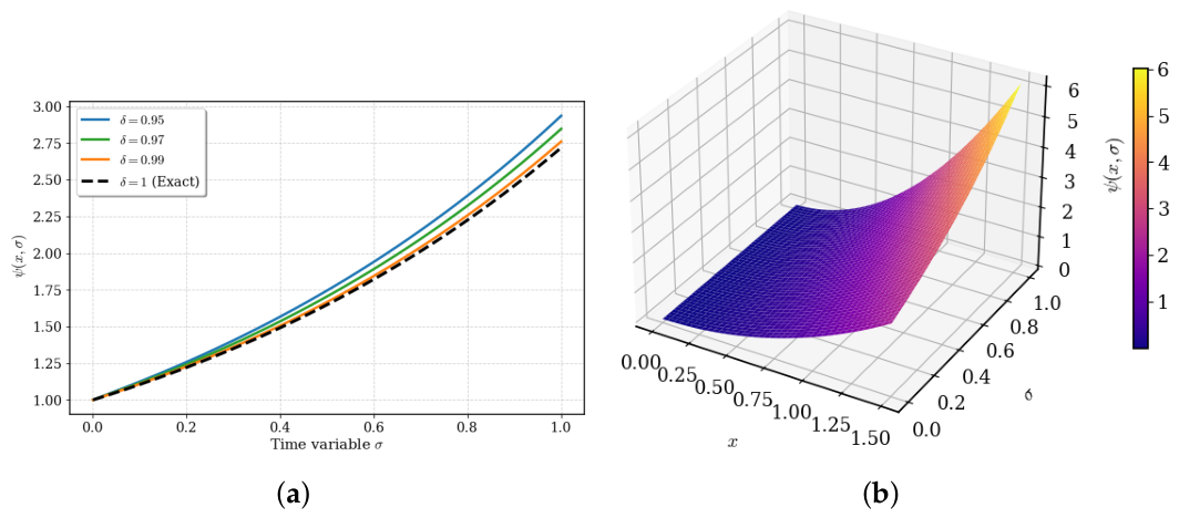
Figure 1a presents a comparison between the exact solution and the obtained numerical solutions of Equation (4) at $x=1$. By taking $\delta =1$, we obtain the exact solution, while for different values of $\delta$ such as $\delta =0.95,0.97,0.99$, we get the approximate fractional solutions.

Figure 1b shows the three-dimensional surface plot of $\psi (x,\sigma )$, illustrating the combined effects of the spatial variable x and the time variable $\sigma$ on the evolution of the solution.

Example 3. 

Let us consider the time-fractional, two-dimensional NSE:

$$\begin{array}{ccc}\hfill D_{\sigma }^{\delta }\varphi +\varphi {\varphi }_{x_1}+\varphi {\omega }_{x_2}& =& {\beta }_0\left({\varphi }_{x_1{x}_1}+{\varphi }_{x_2{x}_2}\right)+k,x_1,x_2,\sigma >0,\hfill \\ \hfill D_{\sigma }^{\delta }\omega +\varphi {\omega }_{x_1}+\omega {\omega }_{x_2}& =& {\beta }_0\left({\omega }_{x_1{x}_1}+{\omega }_{x_2{x}_2}\right)-k,,\hfill \\ \hfill n-1& <& \delta <n;\hfill \end{array}$$

(70)

under the condition

$$\varphi (x_1,x_2,0)=-sin(x_1+x_2),\omega (x_1,x_2,0)=sin(x_1+x_2).$$

By invoking the DNGLT on both sides of Equation (70), we have

$$\begin{array}{ccc}& & N_2^{+}{G}_{\upsilon }\left[D_{\sigma }^{\delta }\varphi +\varphi {\varphi }_{x_1}+\varphi {\omega }_{x_2}={\beta }_0\left({\varphi }_{x_1{x}_1}+{\varphi }_{x_2{x}_2}\right)+k\right]\hfill \\ & & N_2^{+}{G}_{\upsilon }\left[D_{\sigma }^{\delta }\omega +\varphi {\omega }_{x_1}+\omega {\omega }_{x_2}={\beta }_0\left({\omega }_{x_1{x}_1}+{\omega }_{x_2{x}_2}\right)-k\right],\hfill \end{array}$$

From the differentiation property of the natural transform, it follows that

$$\begin{array}{ccc}\hfill {\displaystyle \frac{\Phi (p_1;u,p_2;v,s)}{s^{\delta }}}-s^{\upsilon -\delta +1}\Phi (p_1;u,p_2;v,0)& =& -N_2^{+}{G}_{\upsilon }\left(\varphi {\varphi }_{x_1}+\varphi {\omega }_{x_2}\right)\hfill \\ & & +N_2^{+}{G}_{\upsilon }\left({\beta }_0\left({\varphi }_{x_1{x}_1}+{\varphi }_{x_2{x}_2}\right)+k\right),\hfill \\ \hfill {\displaystyle \frac{\Psi (p_1;u,p_2;v,s)}{s^{\delta }}}-s^{\upsilon -\delta +1}\Psi (p_1;u,p_2;v,0)& =& -N_2^{+}{G}_{\upsilon }\left(\varphi {\omega }_{x_1}+\omega {\omega }_{x_2}\right)\hfill \\ & & +N_2^{+}{G}_{\upsilon }\left({\beta }_0\left({\omega }_{x_1{x}_1}+{\omega }_{x_2{x}_2}\right)-k\right),\hfill \end{array}$$

(71)

By substituting the initial condition and arranging Equation (71), we have

$$\begin{array}{ccc}\hfill \Phi (p_1;u,p_2;v,s)& =& -{\displaystyle \frac{\left(u+v\right)s^{\upsilon +1}}{\left(p_1^2+u^2\right)\left(p_2^2+v^2\right)}}-s^{\delta }{N}_2^{+}{G}_{\upsilon }\left(\varphi {\varphi }_{x_1}+\varphi {\omega }_{x_2}\right)\hfill \\ & & +s^{\delta }{N}_2^{+}{G}_{\upsilon }\left({\beta }_0\left({\varphi }_{x_1{x}_1}+{\varphi }_{x_2{x}_2}\right)+k\right)\hfill \\ \hfill \Psi (p_1;u,p_2;v,s)& =& {\displaystyle \frac{\left(u+v\right)s^{\upsilon +1}}{\left(p_1^2+1\right)\left(p_2^2+1\right)}}-s^{\delta }{N}_2^{+}{G}_{\upsilon }\left(\varphi {\omega }_{x_1}+\omega {\omega }_{x_2}\right)\hfill \\ & & +s^{\delta }{N}_2^{+}{G}_{\upsilon }\left({\beta }_0\left({\omega }_{x_1{x}_1}+{\omega }_{x_2{x}_2}\right)-k\right),\hfill \end{array}$$

(72)

After substituting the initial condition and rearranging Equation (72), we derive

$$\begin{array}{ccc}\hfill \varphi (x_1,x_2,\sigma )& =& -sin(x_1+x_2)-N_2^{-1}{G}_s^{-1}\left(s^{\delta }{N}_2^{+}{G}_{\upsilon }\left(\varphi {\varphi }_{x_1}+\varphi {\omega }_{x_2}\right)\right)\hfill \\ & & +N_2^{-1}{G}_s^{-1}\left(s^{\delta }{N}_2^{+}{G}_{\upsilon }\left({\beta }_0\left({\varphi }_{x_1{x}_1}+{\varphi }_{x_2{x}_2}\right)\right)\right)\hfill \\ & & +{\displaystyle \frac{k{\sigma }^{\delta }}{\Gamma \left(\delta +1\right)}},\hfill \\ \hfill \omega (x_1,x_2,\sigma )& =& sin(x_1+x_2)-N_2^{-1}{G}_s^{-1}\left(s^{\delta }{N}_2^{+}{G}_{\upsilon }\left(\varphi {\omega }_{x_1}+\omega {\omega }_{x_2}\right)\right)\hfill \\ & & +N_2^{-1}{G}_s^{-1}\left(s^{\delta }{N}_2^{+}{G}_{\upsilon }\left({\beta }_0\left({\omega }_{x_1{x}_1}+{\omega }_{x_2{x}_2}\right)\right)\right)\hfill \\ & & -{\displaystyle \frac{k{\sigma }^{\delta }}{\Gamma \left(\delta +1\right)}},\hfill \end{array}$$

(73)

The zeroth components ${\varphi }_0$ and ${\omega }_0$ proposed by the Adomian method always include the initial condition and the source term, both of which are presumed to be known, so we set

$${\varphi }_0=-sin(x_1+x_2)+{\displaystyle \frac{k{\sigma }^{\delta }}{\Gamma \left(\delta +1\right)}},{\omega }_0=sin(x_1+x_2)-{\displaystyle \frac{k{\sigma }^{\delta }}{\Gamma \left(\delta +1\right)}},$$

The remaining components ${\varphi }_{n+1}$, ${\omega }_{n+1},$$n\ge 0$ are given by using the relation

$$\begin{array}{ccc}\hfill {\varphi }_{n+1}& =& -N_2^{-1}{G}_s^{-1}\left(s^{\delta }{N}_2^{+}{G}_{\upsilon }\left(A_n+B_n\right)\right)\hfill \\ & & +N_2^{-1}{G}_s^{-1}\left(\left(s^{\delta }{N}_2^{+}{G}_{\upsilon }\left({\beta }_0\left({\varphi }_{x_1{x}_1}+{\varphi }_{x_2{x}_2}\right)\right)\right)\right),\hfill \end{array}$$

(74)

and

$$\begin{array}{ccc}\hfill {\omega }_{n+1}& =& -N_2^{-1}{G}_s^{-1}\left(s^{\delta }{N}_2^{+}{G}_{\upsilon }\left(C_n+D_n\right)\right)\hfill \\ & & +N_2^{-1}{G}_s^{-1}\left(s^{\delta }{N}_2^{+}{G}_{\upsilon }\left({\beta }_0\left({\omega }_{x_1{x}_1}+{\omega }_{x_2{x}_2}\right)\right)\right)\hfill \end{array}$$

(75)

The first several terms of the Adomian polynomials $A_n,B_n,$$C_n$ and $D_n$ are

$$\begin{array}{ccc}\hfill A_0& =& {\varphi }_0{\varphi }_{0x_1},A_1={\varphi }_0{\varphi }_{1x_1}+{\varphi }_1{\varphi }_{0x_1},\hfill \\ \hfill A_2& =& {\varphi }_0{\varphi }_{2x_1}+{\varphi }_1{\varphi }_{1x_1}+{\varphi }_2{\varphi }_{0x_1},\hfill \\ \hfill A_3& =& {\varphi }_3{\varphi }_{0x_1}+{\varphi }_2{\varphi }_{1x_1}+{\varphi }_1{\varphi }_{2x_1}+{\varphi }_0{\varphi }_{3x_1},\hfill \end{array}$$

(76)

$$\begin{array}{ccc}\hfill B_0& =& {\varphi }_0{\omega }_{0x_2},B_1={\varphi }_0{\omega }_{1x_2}+{\varphi }_1{\omega }_{0x_2},\hfill \\ \hfill B_2& =& {\varphi }_0{\omega }_{2x_2}+{\varphi }_1{\omega }_{1x_2}+{\varphi }_2{\omega }_{0x_2},\hfill \\ \hfill B_3& =& {\varphi }_0{\omega }_{3x_2}+{\varphi }_1{\omega }_{2x_2}+{\varphi }_2{\omega }_{1x_2}+{\varphi }_3{\omega }_{0x_2},\hfill \end{array}$$

(77)

$$\begin{array}{ccc}\hfill C_0& =& {\varphi }_0{\omega }_{0x_1},C_1={\varphi }_0{\omega }_{1x_1}+{\varphi }_1{\omega }_{0x_1},\hfill \\ \hfill C_2& =& {\varphi }_0{\omega }_{2x_1}+{\varphi }_1{\omega }_{1x_1}+{\varphi }_2{\omega }_{0x_1},\hfill \\ \hfill C_3& =& {\varphi }_0{\omega }_{3x_1}+{\varphi }_1{\omega }_{2x_1}+{\varphi }_2{\omega }_{2x_1}+{\varphi }_3{\omega }_{0x_1}.\hfill \end{array}$$

(78)

$$\begin{array}{ccc}\hfill D_0& =& {\omega }_0{\omega }_{0x_2},D_1={\omega }_0{\omega }_{1x_2}+{\omega }_1{\omega }_{0x_2},\hfill \\ \hfill D_2& =& {\omega }_0{\omega }_{2x_2}+{\omega }_1{\omega }_{1x_2}+{\omega }_2{\omega }_{0x_2},\hfill \\ \hfill D_3& =& {\omega }_0{\omega }_{3x_2}+{\omega }_1{\omega }_{2x_2}+{\omega }_2{\omega }_{1x_2}+{\omega }_3{\omega }_{0x_2}.\hfill \end{array}$$

(79)

By putting $n=0$ into Equations (74) and (75), we get

$$\begin{array}{ccc}\hfill {\varphi }_1& =& -N_2^{-1}{G}_s^{-1}\left(s^{\delta }{N}_2^{+}{G}_{\upsilon }\left(A_0+B_0\right)\right)\hfill \\ & & +N_2^{-1}{G}_s^{-1}\left(s^{\delta }{N}_2^{+}{G}_{\upsilon }\left({\beta }_0\left({\varphi }_{0x_1{x}_1}+{\varphi }_{0x_2{x}_2}\right)\right)\right),\hfill \\ & =& N_2^{-1}{G}_s^{-1}\left(s^{\delta }{N}_2^{+}{G}_{\upsilon }\left({\beta }_0\left(2sin(x_1+x_2)\right)\right)\right)\hfill \\ & =& N_2^{-1}{G}_s^{-1}\left(2{\beta }_0{\displaystyle \frac{\left(u+v\right)s^{\upsilon +\delta +1}}{\left(p_1^2+u^2\right)\left(p_2^2+v^2\right)}}\right)\hfill \\ & =& 2{\displaystyle \frac{{\beta }_0{\sigma }^{\delta }}{\Gamma \left(\delta +1\right)}}sin(x_1+x_2)\hfill \end{array}$$

and

$$\begin{array}{ccc}\hfill {\omega }_1& =& -N_2^{-1}{G}_s^{-1}\left(s^{\delta }{N}_2^{+}{G}_{\upsilon }\left(C_0+D_0\right)\right)\hfill \\ & & +N_2^{-1}{G}_s^{-1}\left(s^{\delta }{N}_2^{+}{G}_{\upsilon }\left({\beta }_0\left({\omega }_{0x_1{x}_1}+{\omega }_{0x_2{x}_2}\right)\right)\right)\hfill \\ & =& N_2^{-1}{G}_s^{-1}\left(s^{\delta }{N}_2^{+}{G}_{\upsilon }\left(-2{\beta }_{0}sin(x_1+x_2)\right)\right)\hfill \\ & =& -N_2^{-1}{G}_s^{-1}\left(2{\beta }_0{\displaystyle \frac{\left(u+v\right)s^{\upsilon +\delta +1}}{\left(p_1^2+u^2\right)\left(p_2^2+v^2\right)}}\right)\hfill \\ & =& -2{\displaystyle \frac{{\beta }_0{\sigma }^{\delta }}{\Gamma \left(\delta +1\right)}}sin(x_1+x_2),\hfill \end{array}$$

Similarly, at $n=1,$

$$\begin{array}{ccc}\hfill {\varphi }_2& =& -N_2^{-1}{G}_s^{-1}\left(s^{\delta }{N}_2^{+}{G}_{\upsilon }\left({\varphi }_0{\varphi }_{1x_1}+{\varphi }_1{\varphi }_{0x_1}+{\varphi }_0{\omega }_{1x_2}+{\varphi }_1{\omega }_{0x_2}\right)\right)\hfill \\ & & +N_2^{-1}{G}_s^{-1}\left(s^{\delta }{N}_2^{+}{G}_{\upsilon }\left({\beta }_0\left({\varphi }_{1x_1{x}_1}+{\varphi }_{1x_2{x}_2}\right)\right)\right),\hfill \\ & =& N_2^{-1}{G}_s^{-1}\left(s^{\delta }{N}_2^{+}{G}_{\upsilon }\left({\displaystyle \frac{-4{\beta }_0^{2}sin(x_1+x_2){\sigma }^{\delta }}{\Gamma \left(\delta +1\right)}}\right)\right)\hfill \\ & =& N_2^{-1}{G}_s^{-1}\left(-4{\beta }_0^2{\displaystyle \frac{\left(u+v\right)s^{\upsilon +2\delta +1}}{\left(p_1^2+u^2\right)\left(p_2^2+v^2\right)}}\right)\hfill \\ & =& -{\displaystyle \frac{{\left(2{\beta }_0\right)}^{2}sin(x_1+x_2){\sigma }^{2\delta }}{\Gamma \left(2\delta +1\right)}},\hfill \end{array}$$

and

$$\begin{array}{ccc}\hfill {\omega }_2& =& -N_2^{-1}{G}_s^{-1}\left(s^{\delta }{N}_2^{+}{G}_{\upsilon }\left({\varphi }_0{\omega }_{1x_1}+{\varphi }_1{\omega }_{0x_1}+{\omega }_0{\omega }_{1x_2}+{\omega }_1{\omega }_{0x_2}\right)\right)\hfill \\ & & +N_2^{-1}{G}_s^{-1}\left(s^{\delta }{N}_2^{+}{G}_{\upsilon }\left({\beta }_0\left({\omega }_{1x_1{x}_1}+{\omega }_{1x_2{x}_2}\right)\right)\right)\hfill \\ & =& N_2^{-1}{G}_s^{-1}\left(s^{\delta }{N}_2^{+}{G}_{\upsilon }\left({\displaystyle \frac{4{\beta }_0^{2}sin(x_1+x_2){\sigma }^{\delta }}{\Gamma \left(\delta +1\right)}}\right)\right)\hfill \\ & =& N_2^{-1}{G}_s^{-1}\left(4{\beta }_0^2{\displaystyle \frac{\left(u+v\right)s^{\upsilon +2\delta +1}}{\left(p_1^2+u^2\right)\left(p_2^2+v^2\right)}}\right)\hfill \\ & =& {\displaystyle \frac{{\left(2{\beta }_0\right)}^{2}sin(x_1+x_2){\sigma }^{2\delta }}{\Gamma \left(2\delta +1\right)}},\hfill \end{array}$$

In the same way, at $n=2,$ we have

$$\begin{array}{ccc}\hfill {\varphi }_3& =& -N_2^{-1}{G}_s^{-1}\left(s^{\delta }{N}_2^{+}{G}_{\upsilon }\left(\left({\varphi }_0{\varphi }_{2x_1}+{\varphi }_1{\varphi }_{1x_1}+{\varphi }_2{\varphi }_{0x_1}\right)\right)\right)\hfill \\ & & -N_2^{-1}{G}_s^{-1}\left(s^{\delta }{N}_2^{+}{G}_{\upsilon }\left(\left({\varphi }_0{\omega }_{2x_2}+{\varphi }_1{\omega }_{1x_2}+{\varphi }_2{\omega }_{0x_2}\right)\right)\right)\hfill \\ & & +N_2^{-1}{G}_s^{-1}\left(s^{\delta }{N}_2^{+}{G}_{\upsilon }\left({\beta }_0\left({\varphi }_{2x_1{x}_1}+{\varphi }_{2x_2{x}_2}\right)\right)\right),\hfill \\ & =& N_2^{-1}{G}_s^{-1}\left(s^{\delta }{N}_2^{+}{G}_{\upsilon }\left({\displaystyle \frac{-8{\beta }_0^{3}sin(x_1+x_2){\sigma }^{2\delta }}{\Gamma \left(2\delta +1\right)}}\right)\right)\hfill \\ & =& N_2^{-1}{G}_s^{-1}\left(-8{\beta }_0^3{\displaystyle \frac{\left(u+v\right)s^{\upsilon +2\delta +1}}{\left(p_1^2+u^2\right)\left(p_2^2+v^2\right)}}\right)\hfill \\ & =& {\displaystyle \frac{-8{\beta }_0^{3}sin(x_1+x_2){\sigma }^{3\delta }}{\Gamma \left(3\delta +1\right)}}=-{\displaystyle \frac{{\left(2{\rho }_0\right)}^{3}sin(x_1+x_2){\sigma }^{3\upsilon }}{\Gamma \left(3\delta +1\right)}}\hfill \end{array}$$

And by the same way

$${\omega }_3=-{\displaystyle \frac{{\left(2{\beta }_0\right)}^{3}sin(x_1+x_2){\sigma }^{3\upsilon }}{\Gamma \left(3\delta +1\right)}}.$$

In a similar manner, we have

$${\varphi }_n=-{\displaystyle \frac{{\left(-2{\beta }_0\right)}^{n}sin(x+y){\sigma }^{n\delta }}{\Gamma \left(n\delta +1\right)}},{\omega }_n={\displaystyle \frac{{\left(-2{\beta }_0\right)}^{n}sin(x_1+x_2){\sigma }^{n\delta }}{\Gamma \left(n\delta +1\right)}},\forall n\ge 2.$$

The solution to Equation (70) is given by

$$\begin{array}{ccc}\hfill \varphi (x_1,x_2,\sigma )& =& {\varphi }_0+{\varphi }_1+{\varphi }_2+\dots +{\varphi }_n\hfill \\ \hfill \omega (x_1,x_2,\sigma )& =& {\omega }_0+{\omega }_1+{\omega }_2+\dots +{\omega }_n,\hfill \end{array}$$

$$\begin{array}{ccc}\hfill \varphi (x_1,x_2,\sigma )& =& {\displaystyle -sin(x_1+x_2)\sum _{n=0}^{\infty }\frac{{\left(-2{\beta }_0{\sigma }^{\delta }\right)}^n}{\Gamma \left(n\delta +1\right)}+\frac{k{\sigma }^{\delta }}{\Gamma \left(\delta +1\right)}}\hfill \\ \hfill \omega (x_1,x_2,\sigma )& =& {\displaystyle sin(x_1+x_2)\sum _{n=0}^{\infty }\frac{{\left(-2{\beta }_0{\sigma }^{\delta }\right)}^n}{\Gamma \left(n\delta +1\right)}+\frac{k{\sigma }^{\delta }}{\Gamma \left(\delta +1\right)},}\hfill \end{array}$$

Hence, at $\delta =1$ and $k=0,$ the exact solution of the classical Navier–Stokes equation is given by

$$\begin{array}{ccc}\hfill \varphi (x_1,x_2,\sigma )& =& -sin(x_1+x_2)e^{-2{\beta }_0\sigma }\hfill \\ \hfill \omega (x_1,x_2,\sigma )& =& sin(x_1+x_2)e^{-2{\beta }_0\sigma }.\hfill \end{array}$$

Table 2. Numerical error analysis at $\delta =1$, $k=0$.

Time	Exact Solution	Approximation Solution.	Absolute Error
0.1	−0.818731	0.818731	1.637462
0.2	−0.670320	0.670320	1.340640
0.3	−0.548812	0.548812	1.097623
0.4	−0.449329	0.449329	0.898658
0.5	−0.367879	0.367879	0.735759
$L_2$ Error Norm			$2.65\times {10}^0$
$L_{\infty }$ Error Norm			$1.64\times {10}^0$

illustrates the comparison between the exact solution and the series approximation at $\delta =1$ and $k=0$. It is observed that the approximate solution deviates significantly from the exact solution, as indicated by the relatively large absolute errors. Furthermore, the $L_2$ error norm and $L_{\infty }$ error norm are $2.65$ and $1.64$, respectively.

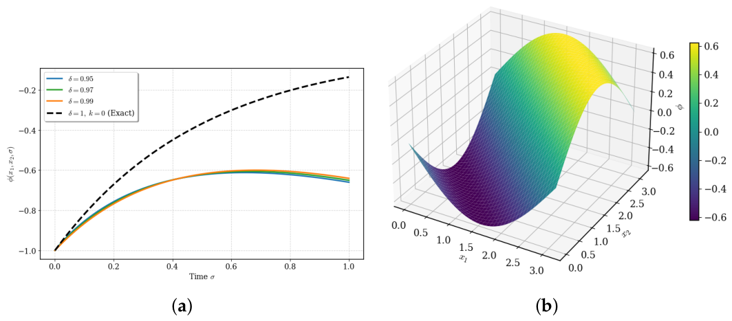
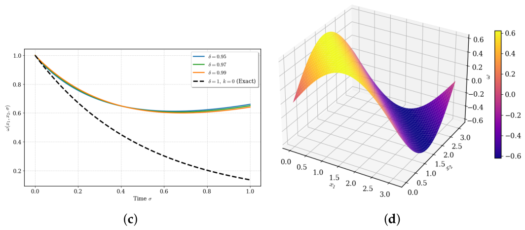
Figure 2a,b present a comparison between the exact solutions and the obtained numerical solutions of $\varphi (x_1,x_2,\sigma )=-sin(x_1+x_2)e^{-2\sigma }$ and $\omega (x_1,x_2,\sigma )=sin(x_1+x_2)e^{-2\sigma }$ at $\sigma =1$. By taking $\sigma =1$, we obtain the exact solutions, while for different values of $\sigma$, we get the approximate solutions.

Figure 2c,d show the three-dimensional plots of the functions $\varphi (x_1,x_2,\sigma )$ and $\omega (x_1,x_2,\sigma )$ at $\sigma =1$, illustrating the combined effects of the spatial variables $x_1$ and $x_2$ on the evolution of the solutions in three dimensions.

6. Conclusions

This article employs the NGLTDM and DNGLTDM techniques for the time-fractional Navier–Stokes system of partial differential equations. These techniques facilitate the resolution of Caputo fractional-order differential equations and yield accurate solutions via iterative processes. We use Theorem 1 to deal with the singularities, Theorem 2 to make sure there is only one solution, and Theorem 3 to look into how solutions converge. Consequently, NGLTDM and DNGLTDM are instrumental in deriving both exact and numerical solutions to fractional NSE.