The Mollification Regularization Method with Truncated Kernels for Solving the Inverse Time-Fractional Schrödinger Problem

Abstract

This paper studies an inverse problem associated with the time-fractional Schrödinger equation in a field-free potential. To address the severe ill-posedness of the problem, a mollification regularization method with truncated kernels is employed to obtain stable approximate solutions. Both a priori and a posteriori strategies for selecting the regularization parameter are developed, and corresponding error estimates for the regularized solutions are derived. The effectiveness of the proposed approach is demonstrated through numerical simulations.

1. Introduction

As a cornerstone of quantum mechanics, the Schrödinger equation provides a fundamental framework for describing the dynamical behavior of microscopic particles and the evolution of their wave functions. It has broad applications in fields such as quantum semiconductors [1], optical pulse propagation [2], and superconductivity [3]. However, when describing open quantum systems, the traditional Schrödinger equation relies on the Markovian approximation, which limits its ability to capture memory effects and spatiotemporal nonlocality in realistic physical systems. In contrast, fractional differential operators possess inherent memory and hereditary properties [4,5,6], offering a rigorous mathematical foundation for modeling such complex dynamics. This has led to steadily growing research interest in the fractional Schrödinger equation.

Numerous methods have been developed for the forward problems of the Schrödinger equation, such as the Krylov projection method [7], the Chebyshev wavelet method [8], the finite difference method [9], the Galerkin finite element method [10], and the collocation method [11,12]. Regarding the inverse problem, various effective numerical methods have also been introduced, including the mollification regularization method [13,14,15], the modified kernel method [16,17], the Landweber iteration method [17,18], the Fourier method [19], and the quasi-boundary regularization method [20]. Among these, the mollification regularization method constructs stable approximate solutions by smoothing perturbed data with appropriate kernel functions. This approach has been widely applied to other ill-posed problems, such as the backward heat conduction problem [21,22], the Cauchy problem for the Helmholtz equation [23], the inverse Laplace transform [24], and the inverse source problem [25,26].

In this paper, we investigate the mollification regularization method for solving the following inverse problem for a time-fractional Schrödinger equation with a potential-free field:

$$\left\{\begin{array}{cc}i{}_0{}^{C}D_t^{\alpha }u(x,t)+u_{xx}(x,t)=0,\hfill & 0\le x<1,t>0,\hfill \\ u(x,0)=0,\hfill & 0\le x<1,\hfill \\ u(1,t)=f(t),\hfill & t\ge 0,\hfill \\ {u(x,t)|}_{x\to \infty }\mathrm{bounded},\hfill & t>0.\hfill \end{array}\right.$$

(1)

Here, i denotes the imaginary unit $\sqrt{-1}$, and ${}_0{}^{C}D_t^{\alpha }u(x,t)$ represents the α-order Caputo time-fractional derivative, formally defined by

$${}_0{}^{C}D_t^{\alpha }u(x,t)={\displaystyle \frac{1}{\mathsf{\Gamma }(1-\alpha )}}{\int }_0^t{(t-\tau )}^{-\alpha }{u}_{\tau }(x,\tau )d\tau ,0<\alpha <1.$$

The objective of the inverse problem is to reconstruct $u(x,t)$ for 0 ≤ x < 1 from the boundary data $u(1,t)=f(t)$. To facilitate the application of Fourier transform techniques, we extend the domain of the variable t in both $f(t)$ and $u(x,t)$ to the real number field $\mathbb{R}$, under the assumption that $f(t)=0$ and $u(x,t)=0$ for all t ≤ 0.

For the integral-order Schrödinger problem, Reference [13] proposes a mollification regularization method employing the Dirichlet kernel, provides both a priori and a posteriori parameter selection strategies, and analyzes the error of corresponding regularized solution. Reference [14] introduces the mollification method with an exponential kernel for solving the same problem. For the time-fractional case, Reference [15] presents a similar Dirichlet kernel-based mollification method along with corresponding parameter selection strategies and error estimates. Since the Dirichlet kernel is a special case of truncated kernel functions, this study proposes a mollification method based on truncated kernel functions for solving the inverse time-fractional Schrödinger problem, thereby extending the framework of Reference [15]. We also establish both a priori and a posteriori parameter selection strategies and derive error estimates for the corresponding regularized solution. Compared with the method in [15], the proposed approach not only offers a generalization but also attains faster convergence rates for the regularized solutions when the Dirichlet kernel is employed.

The remainder of this paper is organized as follows. Section 2 analyzes the ill-posedness of the inverse time-fractional Schrödinger problem via the Fourier transform method. Section 3 introduces a mollification regularization method based on truncated kernels. In Section 4 and Section 5, we present the a priori and a posteriori parameter selection strategies, respectively, along with error estimates for the corresponding regularized solutions. Finally, Section 6 provides numerical simulations to validate the effectiveness of the proposed method.

2. Analysis of the Ill-Posedness

In this section, we analyze the ill-posedness of the inverse time-fractional Schrödinger Problem (1) using the Fourier transform method. For $f(t)\in L^2(\mathbb{R})$, the Fourier transform and its inverse transform are defined as

$$\begin{array}{c}\hfill \widehat{f}(\gamma )={\displaystyle \frac{1}{\sqrt{2\pi }}}{\int }_{-\infty }^{+\infty }f(t)e^{-it\gamma }dt,f(t)={\displaystyle \frac{1}{\sqrt{2\pi }}}{\int }_{-\infty }^{+\infty }\widehat{f}(\gamma )e^{it\gamma }d\gamma .\end{array}$$

Applying the Fourier transform with respect to t to Problem (1) yields

$$\left\{\begin{array}{cc}i{(i\gamma )}^{\alpha }\widehat{u}(x,\gamma )+{\widehat{u}}_{xx}(x,\gamma )=0,\hfill & 0\le x<1,\gamma \in \mathbb{R},\hfill \\ \widehat{u}(x,0)=0,\hfill & 0\le x<1,\hfill \\ \widehat{u}(1,\gamma )=\widehat{f}(\gamma ),\hfill & \gamma \in \mathbb{R}.\hfill \end{array}\right.$$

Its solution is

$$\widehat{u}(x,\gamma )=e^{(1-x)\sqrt{-i{(i\gamma )}^{\alpha }}}\widehat{f}(\gamma ),0\le x<1.$$

Let $\beta (\gamma )=\sqrt{-i{(i\gamma )}^{\alpha }}={\beta }_1(\gamma )+i{\beta }_2(\gamma )$, where

$$\begin{array}{cc}\hfill {\beta }_1(\gamma )& =\sqrt{{\displaystyle \frac{{|\gamma |}^{\alpha }}{2}}(1+sign(\gamma )sin({\displaystyle \frac{\alpha \pi }{2}}))},\hfill \\ \hfill {\beta }_2(\gamma )& =-\sqrt{{\displaystyle \frac{{|\gamma |}^{\alpha }}{2}}(1-sign(\gamma )sin({\displaystyle \frac{\alpha \pi }{2}}))},\hfill \end{array}$$

we obtain

$$\widehat{u}(x,\gamma )=e^{(1-x)\beta (\gamma )}\widehat{f}(\gamma ),0\le x<1,$$

(2)

Thus, the exact solution of Problem (1) is given by

$$\begin{array}{c}\hfill u(x,t)={\displaystyle \frac{1}{\sqrt{2\pi }}}{\int }_{-\infty }^{+\infty }\widehat{f}(\gamma )e^{(1-x)\beta (\gamma )}{e}^{i\gamma t}d\gamma ,0\le x<1.\end{array}$$

(3)

In practical applications, the exact function $f(t)$ is generally unavailable; only perturbed measurement data $f^{\delta }(t)$ can be obtained. We assume that

$$\parallel f^{\delta }(·)-f(·)\parallel \le \delta ,$$

(4)

where $\parallel ·\parallel$ denotes the L²-norm and δ > 0 represents the noise level. For a given data $f^{\delta }(t)$, we denote the corresponding regularized solution by $u^{\delta }(x,t)$. To illustrate the ill-posedness of the inverse time-fractional Schrödinger problem, we consider a specific example. Suppose the perturbed data are given by

$$f^{\delta }(t)=f(t)+\sqrt{{\displaystyle \frac{2}{\pi }}}·{\displaystyle \frac{sin(nt)}{nt}}.$$

For 0 ≤ x < 1 and 0 < α < 1, Parseval’s identity yields

$$\begin{array}{c}\hfill {∥f^{\delta }(·)-f(·)∥}^2={\displaystyle \frac{2}{\pi }}{\parallel {\displaystyle \frac{sin(nt)}{nt}}\parallel }^2={\int }_{-n}^n{\displaystyle \frac{1}{n^2}}d\gamma ={\displaystyle \frac{2}{n}}\to 0,n\to +\infty ,\end{array}$$

and

$$\begin{array}{cc}\hfill {∥u^{\delta }(x,·)-u(x,·)∥}^2& ={∥{\widehat{u}}^{\delta }(x,·)-\widehat{u}(x,·)∥}^2\hfill \\ \hfill & ={\displaystyle \frac{2}{\pi }}{∥\widehat{{\displaystyle \frac{sin(nt)}{nt}}}{e}^{(1-x)\beta (\gamma )}∥}^2\hfill \\ \hfill & ={\int }_{-n}^n{\displaystyle \frac{{\left|e^{(1-x)\beta (\gamma )}\right|}^2}{n^2}}d\gamma \hfill \\ \hfill & \ge {\displaystyle \frac{{\int }_{\frac{n}{2}}^n{e}^{2(1-x){\beta }_1(\gamma )}d\gamma }{n^2}}\hfill \\ \hfill & \ge {\displaystyle \frac{e^{(1-x)n^{\alpha /2}}}{n^2}}\to +\infty ,n\to +\infty .\hfill \end{array}$$

It is clear that the error in the perturbed data converges to zero, whereas the error in the solution diverges to infinity as n → ∞. This confirms the ill-posedness of the inverse time-fractional Schrödinger problem.

3. The Mollification Method with Truncated Kernel Functions

In this section, we introduce the definition of truncated kernel functions and the associated mollification regularization method.

First, recall the definition of convolution:

$$\begin{array}{c}\hfill (Q_{\mu }\ast f)(t)={\int }_{-\infty }^{+\infty }{Q}_{\mu }(s)f(t-s)ds={\int }_{-\infty }^{+\infty }{Q}_{\mu }(t-s)f(s)ds.\end{array}$$

By the convolution theorem, we have

$$\begin{array}{c}\hfill \widehat{(Q_{\mu }\ast f)}(\gamma )=\sqrt{2\pi }{\widehat{Q}}_{\mu }(\gamma )\widehat{f}(\gamma ).\end{array}$$

Convolving the perturbed data $f^{\delta }(t)$ with the kernel $Q_{\mu }(t)$ leads to the modified problem:

$$\left\{\begin{array}{cc}i{}_0{}^{C}D_t^{\alpha }{u}^{\mu ,\delta }(x,t)+u_{xx}^{\mu ,\delta }(x,t)=0,\hfill & 0\le x<1,t>0,\hfill \\ u^{\mu ,\delta }(x,0)=0,\hfill & 0\le x<1,\hfill \\ u^{\mu ,\delta }(1,t)=(Q_{\mu }\ast f^{\delta })(t),\hfill & t\ge 0,\hfill \\ u^{\mu ,\delta }{(x,t)|}_{x\to \infty }\mathrm{bounded},\hfill & t>0.\hfill \end{array}\right.$$

(5)

Solving (5) in the frequency domain gets

$$\begin{array}{c}\hfill {\widehat{u}}^{\mu ,\delta }(x,\gamma )=(\widehat{Q_{\mu }\ast f^{\delta }})(\gamma )e^{(1-x)\beta (\gamma )}={\widehat{P}}_{\mu }(\gamma )e^{(1-x)\beta (\gamma )}{\widehat{f}}^{\delta }(\gamma ),\end{array}$$

(6)

where ${\widehat{P}}_{\mu }(\gamma )=\sqrt{2\pi }{\widehat{Q}}_{\mu }(\gamma )$. Applying the inverse Fourier transform yields the regularized solution

$$\begin{array}{c}\hfill u^{\mu ,\delta }(x,t)={\displaystyle \frac{1}{\sqrt{2\pi }}}{\int }_{-\infty }^{+\infty }{\widehat{P}}_{\mu }(\gamma )e^{(1-x)\beta (\gamma )}{\widehat{f}}^{\delta }(\gamma )e^{i\gamma t}d\gamma .\end{array}$$

(7)

In the subsequent analysis, we assume $\parallel {\widehat{f}}^{\delta }\parallel \ne 0$ without loss of generality. If $\parallel {\widehat{f}}^{\delta }\parallel =0$, the regularization term vanishes identically, rendering the regularization ineffective.

Next, we define the truncated kernel function employed in the mollification regularization method for solving the inverse time-fractional Schrödinger problem (1).

Definition 1.

For $0\le x<1$, a kernel function ${\widehat{P}}_{\mu }(\gamma )(\gamma \in \mathbb{R})$ is called a truncated kernel function if it satisfies the following two conditions:

• $(1)\left|{\widehat{P}}_{\mu }(\gamma )e^{(1-x)\beta (\gamma )}\right|\le e^{{\displaystyle \frac{1-x}{\sqrt{{(\mu /c)}^{\alpha }}}}}$;
  $(2)\left|\left(1-{\widehat{P}}_{\mu }(\gamma )\right)e^{-x\beta (\gamma )}\right|\le e^{{\displaystyle \frac{-bx}{\sqrt{{\mu }^{\alpha }}}}}$,

where $c>0$ is a constant and $b=\sqrt{{\displaystyle \frac{1-sin(\alpha \pi /2)}{2}}}>0$.

Lemma 1.

Both the Dirichlet kernel

$${\widehat{P}}_{\mu }(\gamma )={\chi }_{\left[-{\displaystyle \frac{1}{\mu }},{\displaystyle \frac{1}{\mu }}\right]}(\gamma )$$

and the Poussin kernel

$${\widehat{P}}_{\mu }(\gamma )=\left\{\begin{array}{cc}1,\hfill & |\gamma |\le {\displaystyle \frac{1}{\mu }},\hfill \\ 2-\mu |\gamma |,\hfill & {\displaystyle \frac{1}{\mu }}\le |\gamma |<{\displaystyle \frac{2}{\mu }},\hfill \\ 0,\hfill & |\gamma |\ge {\displaystyle \frac{2}{\mu }}\hfill \end{array}\right.$$

are truncated kernel functions.

Proof. 

We first consider the Dirichlet kernel

$${\widehat{P}}_{\mu }(\gamma )={\chi }_{\left[-{\displaystyle \frac{1}{\mu }},{\displaystyle \frac{1}{\mu }}\right]}(\gamma ).$$

Case 1: $|\gamma |\le {\displaystyle \frac{1}{\mu }}$.

Here ${\widehat{P}}_{\mu }(\gamma )=1$; so

$$\left|{\widehat{P}}_{\mu }(\gamma )e^{(1-x)\beta (\gamma )}\right|=\left|e^{(1-x)({\beta }_1(\gamma )+i{\beta }_2(\gamma ))}\right|=e^{(1-x){\beta }_1(\gamma )}\le e^{{\displaystyle \frac{1-x}{\sqrt{{\mu }^{\alpha }}}}},$$

and

$$\left|\left(1-{\widehat{P}}_{\mu }(\gamma )\right)e^{-x\beta (\gamma )}\right|=0.$$

Case 2: $|\gamma |>{\displaystyle \frac{1}{\mu }}$.

Now ${\widehat{P}}_{\mu }(\gamma )=0$; hence

$$\left|{\widehat{P}}_{\mu }(\gamma )e^{(1-x)\beta (\gamma )}\right|=0,$$

and

$$\left|\left(1-{\widehat{P}}_{\mu }(\gamma )\right)e^{-x\beta (\gamma )}\right|=e^{-x{\beta }_1(\gamma )}\le e^{{\displaystyle \frac{-bx}{\sqrt{{\mu }^{\alpha }}}}}.$$

Thus, the Dirichlet kernel satisfies both conditions of Definition 1 with the constant c = 1; hence it is a truncated kernel function.

Next, we consider the Poussin kernel

$${\widehat{P}}_{\mu }(\gamma )=\sqrt{2\pi }{\widehat{Q}}_{\mu }(\gamma )=\left\{\begin{array}{cc}1,\hfill & |\gamma |\le {\displaystyle \frac{1}{\mu }},\hfill \\ 2-\mu |\gamma |,\hfill & {\displaystyle \frac{1}{\mu }}\le |\gamma |<{\displaystyle \frac{2}{\mu }},\hfill \\ 0,\hfill & |\gamma |\ge {\displaystyle \frac{2}{\mu }}.\hfill \end{array}\right.$$

Case 1: $|\gamma |\le {\displaystyle \frac{1}{\mu }}$.

Here ${\widehat{P}}_{\mu }(\gamma )=1$; thus

$$\left|{\widehat{P}}_{\mu }(\gamma )e^{(1-x)\beta (\gamma )}\right|=\left|e^{(1-x)({\beta }_1(\gamma )+i{\beta }_2(\gamma ))}\right|=e^{(1-x){\beta }_1(\gamma )}\le e^{{\displaystyle \frac{1-x}{\sqrt{{\mu }^{\alpha }}}}},$$

and

$$\left|\left(1-{\widehat{P}}_{\mu }(\gamma )\right)e^{-x\beta (\gamma )}\right|=0.$$

Case 2: ${\displaystyle \frac{1}{\mu }}\le |\gamma |<{\displaystyle \frac{2}{\mu }}$.

In this interval, $0<2-\mu |\gamma |\le 1$. Consequently,

$$\left|{\widehat{P}}_{\mu }(\gamma )e^{(1-x)\beta (\gamma )}\right|=\left|e^{(1-x)({\beta }_1(\gamma )+i{\beta }_2(\gamma ))}\right|=e^{(1-x){\beta }_1(\gamma )}\le e^{{\displaystyle \frac{1-x}{\sqrt{{(\mu /2)}^{\alpha }}}}},$$

and

$$\left|\left(1-{\widehat{P}}_{\mu }(\gamma )\right)e^{-x\beta (\gamma )}\right|=\left|(\mu |\gamma |-1)e^{-x({\beta }_1(\gamma )+i{\beta }_2(\gamma ))}\right|\le e^{-x{\beta }_1(\gamma )}\le e^{{\displaystyle \frac{-bx}{\sqrt{{\mu }^{\alpha }}}}}.$$

Case 3: $|\gamma |\ge {\displaystyle \frac{2}{\mu }}$.

Here ${\widehat{P}}_{\mu }(\gamma )=1$; hence

$$\left|{\widehat{P}}_{\mu }(\gamma )e^{(1-x)\beta (\gamma )}\right|=0,$$

and

$$\left|\left(1-{\widehat{P}}_{\mu }(\gamma )\right)e^{-x\beta (\gamma )}\right|=\left|e^{-x({\beta }_1(\gamma )+i{\beta }_2(\gamma ))}\right|=e^{-x{\beta }_1(\gamma )}\le e^{{\displaystyle \frac{-bx}{\sqrt{{\mu }^{\alpha }}}}}.$$

Thus, the Poussin kernel also satisfies both conditions of Definition 1 with the constant $c=2$; therefore it is a truncated kernel function. □

Indeed, the general form of a truncated kernel function can be expressed as

$${\widehat{P}}_{\mu }(\gamma )=\left\{\begin{array}{cc}1,\hfill & |\gamma |\le {\displaystyle \frac{1}{\mu }},\hfill \\ k(\mu ,\gamma ),\hfill & {\displaystyle \frac{1}{\mu }}\le |\gamma |<{\displaystyle \frac{2}{\mu }},\hfill \\ 0,\hfill & |\gamma |\ge {\displaystyle \frac{2}{\mu }},\hfill \end{array}\right.$$

where $0\le k(\mu ,\gamma )\le 1$. Following a proof analogous to that of the Poussin kernel in Lemma 1, the constant c in Definition 1 can be taken as c = 2. Different choices of the function $k(\mu ,\gamma )$ yield various truncated kernel functions. For example, the exponential truncated kernel can be defined by

$$k(\mu ,\gamma )={\displaystyle \frac{1}{1-e}}(1-e^{1-{(|\gamma |\mu -1)}^m}),m>0,$$

and the power truncated kernel is defined by

$$k(\mu ,\gamma )={\displaystyle \frac{2}{1+{(|\gamma |\mu -1)}^m}}-1,m>0,$$

where the parameter m controls the rate of change of $k(\mu ,\gamma )$.

To derive the error estimate for the regularized solution given in (7), certain a priori assumptions on the initial data $u(0,·)$ must be introduced. We assume that $u(0,·)$ satisfies

$$\begin{array}{c}\hfill {∥u(0,·)∥}_{S^p(\mathbb{R})}\le E_p,p\ge 0,\end{array}$$

(8)

where $E_p>0$ is a constant. The norm ${∥·∥}_{S^p(\mathbb{R})}$ is defined by

$$\begin{array}{c}\hfill {∥u(0,·)∥}_{S^p(\mathbb{R})}=({\int }_{-\infty }^{+\infty }{e}^{p{\beta }_1(\gamma )}|\widehat{u}(0,\gamma ){{|}^{2}d\gamma )}^{{\displaystyle \frac{1}{2}}}.\end{array}$$

It is readily seen that $S^0(\mathbb{R})=L^2(\mathbb{R})$ when $p=0$.

4. Error Estimate with a Priori Parameter Selection Strategy

In this section, we derive an error estimate for the regularized solution $u^{\mu ,\delta }(x,t)$ when the regularization parameter $\mu =\mu (\delta )$ is chosen by an a priori strategy. First, we consider the case 0 < x < 1.

Theorem 1.

Let ${\widehat{P}}_{\mu }(\gamma )(\gamma \in \mathbb{R})$ be a truncated kernel function. If the noise condition (4) holds and the a priori condition (8) is satisfied with $p=0$ when $0<x<1$, then

$$\begin{array}{c}\hfill ∥u^{\mu ,\delta }(x,·)-u(x,·)∥\le \delta e^{{({\displaystyle \frac{c}{\mu }})}^{{\displaystyle \frac{\alpha }{2}}}(1-x)}+E{e}^{{\displaystyle \frac{-bx}{{\mu }^{\alpha /2}}}}.\end{array}$$

In particular, if we choose

$$\begin{array}{c}\hfill \mu ={\left({\displaystyle \frac{1}{\sqrt{c^{\alpha }}(1-x)+bx}}ln({\displaystyle \frac{E_0}{\delta }})\right)}^{-{\displaystyle \frac{2}{\alpha }}},\end{array}$$

then

$$\begin{array}{c}\hfill ∥u^{\mu ,\delta }(x,·)-u(x,·)∥\le C_1{\delta }^{{\displaystyle \frac{bx}{\sqrt{c^{\alpha }}(1-x)+bx}}},\end{array}$$

where $C_1=2E_0^{{\displaystyle \frac{\sqrt{c^{\alpha }}(1-x)}{\sqrt{c^{\alpha }}(1-x)+bx}}}.$

Proof. 

Using Parseval’s identity and the triangle inequality, we have

$$\begin{array}{cc}\hfill ∥u^{\mu ,\delta }(x,·)-u(x,·)∥& =∥{\widehat{u}}^{\mu ,\delta }(x,·)-\widehat{u}(x,·)∥\hfill \\ \hfill & \le ∥{\widehat{u}}^{\mu ,\delta }(x,·)-{\widehat{u}}^{\mu ,0}(x,·)∥+∥{\widehat{u}}^{\mu ,0}(x,·)-\widehat{u}(x,·)∥\hfill \\ \hfill & =∥{\widehat{P}}_{\mu }(\gamma )e^{(1-x)\beta (\gamma )}\left({\widehat{f}}^{\delta }(\gamma )-\widehat{f}(\gamma )\right)∥\hfill \\ \hfill & +∥\left(1-{\widehat{P}}_{\mu }(\gamma )\right)e^{(1-x)\beta (\gamma )}\widehat{f}(\gamma )∥\hfill \\ \hfill & \le e^{{\displaystyle \frac{1-x}{\sqrt{{(\mu /c)}^{\alpha }}}}}\delta +∥\left(1-{\widehat{P}}_{\mu }(\gamma )\right)e^{-x\beta (\gamma )}{e}^{\beta (\gamma )}\widehat{f}(\gamma )∥\hfill \\ \hfill & \le e^{{\displaystyle \frac{1-x}{\sqrt{{(\mu /c)}^{\alpha }}}}}\delta +e^{{\displaystyle \frac{-bx}{\sqrt{{\mu }^{\alpha }}}}}\parallel \widehat{u}(0,·)\parallel \hfill \\ \hfill & \le e^{{\displaystyle \frac{1-x}{\sqrt{{(\mu /c)}^{\alpha }}}}}\delta +e^{{\displaystyle \frac{-bx}{\sqrt{{\mu }^{\alpha }}}}}{E}_0.\hfill \end{array}$$

Let $\mu ={\left({\displaystyle \frac{1}{\sqrt{c^{\alpha }}(1-x)+bx}}ln\left({\displaystyle \frac{E_0}{\delta }}\right)\right)}^{-{\displaystyle \frac{2}{\alpha }}}$; then we have

$$\begin{array}{c}\hfill ∥u^{\mu ,\delta }(x,·)-u(x,·)∥\le 2E_0^{{\displaystyle \frac{\sqrt{c^{\alpha }}(1-x)}{\sqrt{c^{\alpha }}(1-x)+bx}}}{\delta }^{{\displaystyle \frac{bx}{\sqrt{c^{\alpha }}(1-x)+bx}}}.\end{array}$$

□

Next, we consider the case x = 0. To obtain a convergence rate for the regularized solution $u^{\mu ,\delta }(0,·)$, a stronger a priori assumption on the initial data $u(0,·)$ is required.

Theorem 2.

Let ${\widehat{P}}_{\mu }(\gamma )(\gamma \in \mathbb{R})$ be a truncated kernel function. If the noise condition (4) holds and the a priori condition (8) is satisfied with some $p>0$, then

$$\begin{array}{c}\hfill ∥u^{\mu ,\delta }(0,·)-u(0,·)∥\le e^{{({\displaystyle \frac{c}{\mu }})}^{{\displaystyle \frac{\alpha }{2}}}}\delta +e^{{\displaystyle \frac{-pb}{2{\mu }^{\alpha /2}}}}{E}_p,\end{array}$$

In particular, if we choose

$$\begin{array}{c}\hfill \mu ={\left({\displaystyle \frac{2}{2\sqrt{c^{\alpha }}+pb}}ln({\displaystyle \frac{E_p}{\delta }})\right)}^{-{\displaystyle \frac{2}{\alpha }}},\end{array}$$

then

$$\begin{array}{c}\hfill ∥u^{\mu ,\delta }(0,·)-u(0,·)∥\le C_2{\delta }^{{\displaystyle \frac{pb}{2\sqrt{c^{\alpha }}+pb}}},\end{array}$$

where $C_2=2E_p^{{\displaystyle \frac{2\sqrt{c^{\alpha }}}{2\sqrt{c^{\alpha }}+pb}}}.$

Proof. 

Using Parseval’s identity and the triangle inequality, we have

$$\begin{array}{cc}\hfill ∥u^{\mu ,\delta }(0,·)-u(0,·)∥& =∥{\widehat{u}}^{\mu ,\delta }(0,\gamma )-\widehat{u}(0,\gamma )∥\hfill \\ \hfill & \le ∥{\widehat{u}}^{\mu ,\delta }(0,\gamma )-{\widehat{u}}^{\mu ,0}(0,\gamma )∥+∥{\widehat{u}}^{\mu ,0}(0,\gamma )-\widehat{u}(0,\gamma )∥\hfill \\ \hfill & =∥{\widehat{P}}_{\mu }(\gamma )e^{\beta (\gamma )}\left({\widehat{f}}^{\delta }(\gamma )-\widehat{f}(\gamma )\right)∥+∥\left(1-{\widehat{P}}_{\mu }(\gamma )\right)e^{\beta (\gamma )}\widehat{f}(\gamma )∥\hfill \\ \hfill & \le e^{{\displaystyle \frac{1}{\sqrt{{(\mu /c)}^{\alpha }}}}}\delta +∥\left(1-{\widehat{P}}_{\mu }(\gamma )\right)e^{-{\displaystyle \frac{p}{2}}\beta (\gamma )}{e}^{{\displaystyle \frac{p}{2}}\beta (\gamma )}\widehat{u}(0,\gamma )∥\hfill \\ \hfill & \le e^{{\displaystyle \frac{1}{\sqrt{{(\mu /c)}^{\alpha }}}}}\delta +e^{{\displaystyle \frac{-pb}{2\sqrt{{\mu }^{\alpha }}}}}{E}_p.\hfill \end{array}$$

Let $\mu ={\left({\displaystyle \frac{2}{2\sqrt{c^{\alpha }}+pb}}ln({\displaystyle \frac{E_p}{\delta }})\right)}^{-{\displaystyle \frac{2}{\alpha }}}$; then we have

$$\begin{array}{c}\hfill ∥u^{\mu ,\delta }(0,·)-u(0,·)∥\le 2E_p^{{\displaystyle \frac{2\sqrt{c^{\alpha }}}{2\sqrt{c^{\alpha }}+pb}}}{\delta }^{{\displaystyle \frac{pb}{2\sqrt{c^{\alpha }}+pb}}}.\end{array}$$

□

5. Error Estimate with a Posteriori Parameter Selection Strategy

The a priori parameter choice requires specific assumptions on the initial data $u(0,·)$, such as $E_0$ in Theorem 1 and $E_p$ in Theorem 2. To overcome this limitation, this section introduces an a posteriori selection strategy for the regularization parameter based on Morozov’s discrepancy principle. We first state the following lemma.

Lemma 2.

Define $h(\mu )=∥(1-{\widehat{P}}_{\mu }(\gamma )){\widehat{f}}^{\delta }(\gamma )∥$. Then the following properties hold:

$(1)$ The function $h(\mu )$ is continuous;

$(2)$ The function $h(\mu )$ is monotonically increasing;

$(3){lim}_{\mu \to 0^{+}}h(\mu )=0$;

$(4){lim}_{\mu \to +\infty }h(\mu )=∥{\widehat{f}}^{\delta }∥$;

The proof of Lemma 2 is straightforward and is omitted here. Let

$$\begin{array}{c}\hfill ∥(1-{\widehat{P}}_{\mu }(\gamma )){\widehat{f}}^{\delta }(\gamma )∥=\delta +\tau {\delta }^{{\displaystyle \frac{b}{\sqrt{c^{\alpha }}}}},\end{array}$$

(9)

where $\tau >0$ is chosen so that

$$0<\delta +\tau {\delta }^{{\displaystyle \frac{b}{\sqrt{c^{\alpha }}}}}<∥{\widehat{f}}^{\delta }∥.$$

(10)

By Lemma 2 and Condition (10), Equation (9) admits a unique solution $\mu =\mu (\delta )$. The a posteriori parameter selection strategy is then defined by taking this $\mu (\delta )$ as the regularization parameter.

Lemma 3.

When $0\le x<1$, assume that the noise condition (4) holds and the a priori condition (8) is satisfied for some $p\ge 0$. Then

$$\begin{array}{c}\hfill \delta e^{{\displaystyle \frac{p+2}{2\sqrt{{(\mu /c)}^{\alpha }}}}}\le {\left({\displaystyle \frac{E_p}{\tau }}\right)}^{{\displaystyle \frac{\sqrt{c^{\alpha }}}{b}}}.\end{array}$$

Proof. 

Using the triangle inequality, we obtain

$$\begin{array}{cc}\hfill \delta +\tau {\delta }^{{\displaystyle \frac{b}{\sqrt{c^{\alpha }}}}}& =∥\left(1-{\widehat{P}}_{\mu }(\gamma )\right){\widehat{f}}^{\delta }(\gamma )∥\hfill \\ \hfill & \le ∥\left(1-{\widehat{P}}_{\mu }(\gamma )\right)\left({\widehat{f}}^{\delta }(\gamma )-\widehat{f}(\gamma )\right)∥+∥\left(1-{\widehat{P}}_{\mu }(\gamma )\right)\widehat{f}(\gamma )∥\hfill \\ \hfill & \le \delta +∥\left(1-{\widehat{P}}_{\mu }(\gamma )\right)e^{-{\displaystyle \frac{p+2}{2}}\beta (\gamma )}{e}^{{\displaystyle \frac{p}{2}}\beta (\gamma )}{e}^{\beta (\gamma )}\widehat{f}(\gamma )∥\hfill \\ \hfill & \le \delta +∥\left(1-{\widehat{P}}_{\mu }(\gamma )\right)e^{-{\displaystyle \frac{p+2}{2}}\beta (\gamma )}{e}^{{\displaystyle \frac{p}{2}}\beta (\gamma )}\widehat{u}(0,\gamma )∥\hfill \\ \hfill & \le \delta +e^{-{\displaystyle \frac{(p+2)b}{2\sqrt{{\mu }^{\alpha }}}}}{E}_p.\hfill \end{array}$$

Hence

$$\begin{array}{cc}\hfill {\delta }^{{\displaystyle \frac{b}{\sqrt{c^{\alpha }}}}}{e}^{{\displaystyle \frac{(p+2)b}{2\sqrt{{\mu }^{\alpha }}}}}& \le {\displaystyle \frac{E_p}{\tau }},\hfill \end{array}$$

and then

$$\begin{array}{c}\hfill \delta e^{{\displaystyle \frac{p+2}{2\sqrt{{(\mu /c)}^{\alpha }}}}}\le {\left({\displaystyle \frac{E_p}{\tau }}\right)}^{{\displaystyle \frac{\sqrt{c^{\alpha }}}{b}}}.\end{array}$$

□

Theorem 3.

When $0<x<1$, assume that the noise condition (4) holds and the a priori condition (8) is satisfied with $p=0$. If the regularization parameter $\mu =\mu (\delta )$ is chosen as the unique solution of (9), then

$$\begin{array}{c}\hfill ∥u^{\mu ,\delta }(x,·)-u(x,·)∥\le C_3{\delta }^{{\displaystyle \frac{bx}{\sqrt{c^{\alpha }}}}},\end{array}$$

where $C_3={\left(\tau +o(1)\right)}^x{\left({({\displaystyle \frac{E_0}{\tau }})}^{{\displaystyle \frac{\sqrt{c^{\alpha }}}{b}}}+E_0\right)}^{1-x}.$

Proof. 

Using Parseval’s identity and Hölder’s inequality, we have

$$\begin{array}{cc}\hfill & ∥u^{\mu ,\delta }(x,·)-u(x,·)∥=∥{\widehat{u}}^{\mu ,\delta }(x,·)-\widehat{u}(x,·)∥\hfill \\ \hfill & =∥e^{(1-x)\beta (\gamma )}\left({\widehat{P}}_{\mu }(\gamma ){\widehat{f}}^{\delta }(\gamma )-\widehat{f}(\gamma )\right)∥\hfill \\ \hfill & \le {∥{\widehat{P}}_{\mu }(\gamma ){\widehat{f}}^{\delta }(\gamma )-\widehat{f}(\gamma )∥}^x{∥e^{\beta (\gamma )}\left({\widehat{P}}_{\mu }(\gamma ){\widehat{f}}^{\delta }(\gamma )-\widehat{f}(\gamma )\right)∥}^{1-x}\hfill \\ \hfill & \le {\left(∥{\widehat{P}}_{\mu }(\gamma ){\widehat{f}}^{\delta }(\gamma )-{\widehat{f}}^{\delta }(\gamma )∥+∥{\widehat{f}}^{\delta }(\gamma )-\widehat{f}(\gamma )∥\right)}^x\hfill \\ \hfill & ·{∥e^{\beta (\gamma )}\left({\widehat{P}}_{\mu }(\gamma ){\widehat{f}}^{\delta }(\gamma )-\widehat{f}(\gamma )\right)∥}^{1-x}\hfill \\ \hfill & \le {\left(\tau {\delta }^{{\displaystyle \frac{b}{\sqrt{c^{\alpha }}}}}+2\delta \right)}^x(∥e^{\beta (\gamma )}{\widehat{P}}_{\mu }(\gamma )\left({\widehat{f}}^{\delta }(\gamma )-\widehat{f}(\gamma )\right)∥\hfill \\ \hfill & +∥\left({\widehat{P}}_{\mu }(\gamma )-1\right)e^{\beta (\gamma )}\widehat{f}(\gamma )∥{)}^{1-x}\hfill \\ \hfill & \le {\left(\tau {\delta }^{{\displaystyle \frac{b}{\sqrt{c^{\alpha }}}}}+2\delta \right)}^x{\left(e^{{\displaystyle \frac{1}{\sqrt{{(\mu /c)}^{\alpha }}}}}\delta +E_0\right)}^{1-x}\hfill \\ \hfill & \le {\delta }^{{\displaystyle \frac{bx}{\sqrt{c^{\alpha }}}}}{\left(\tau +2{\delta }^{1-{\displaystyle \frac{b}{\sqrt{c^{\alpha }}}}}\right)}^x{\left({({\displaystyle \frac{E_0}{\tau }})}^{{\displaystyle \frac{\sqrt{c^{\alpha }}}{b}}}+E_0\right)}^{1-x}\hfill \\ \hfill & ={\delta }^{{\displaystyle \frac{bx}{\sqrt{c^{\alpha }}}}}{\left(\tau +o(1)\right)}^x{\left({({\displaystyle \frac{E_0}{\tau }})}^{{\displaystyle \frac{\sqrt{c^{\alpha }}}{b}}}+E_0\right)}^{1-x}.\hfill \end{array}$$

□

Remark 1.

The convergence rate of the regularized solution with a posteriori parameter selection in Theorem 3 is $O({\delta }^{{\displaystyle \frac{bx}{\sqrt{c^{\alpha }}}}})$, whereas the rate with a priori selection in Theorem 1 is $O({\delta }^{{\displaystyle \frac{bx}{\sqrt{c^{\alpha }}(1-x)+bx}}})$. Since

$$b=\sqrt{(1-sin(\alpha \pi /2))/2}\in (0,{\displaystyle \frac{1}{\sqrt{2}}})$$

and for the Dirichlet kernel we have $c=1$ while for other truncated kernels $c=2$, it follows that $\sqrt{c^{\alpha }}(1-x)+bx<\sqrt{c^{\alpha }}$, which means the a priori convergence rate is faster than the a posteriori rate. Furthermore, the a priori convergence rate for the Dirichlet kernel given in Reference [15] is $O({\delta }^{bx})$, which coincides with the a posteriori convergence rate in the present work but is slower than the a priori rate obtained here.

Theorem 4.

When $x=0$, assume that the noise condition (4) holds and the a priori condition (8) is satisfied with some $p>0$. If the regularization parameter $\mu =\mu (\delta )$ is chosen as the unique solution of (9), then

$$\begin{array}{c}\hfill ∥u^{\mu ,\delta }(0,·)-u(0,·)∥\le C_4{\delta }^{{\displaystyle \frac{pb}{(p+2)\sqrt{c^{\alpha }}}}},\end{array}$$

where $C_4={\left(\tau +o(1)\right)}^{{\displaystyle \frac{p}{p+2}}}{\left({({\displaystyle \frac{E_p}{\tau }})}^{{\displaystyle \frac{\sqrt{c^{\alpha }}}{b}}}+E_p\right)}^{{\displaystyle \frac{2}{p+2}}}.$

Proof. 

Using Parseval’s identity and Hölder’s inequality, we have

$$\begin{array}{cc}\hfill & ∥u^{\mu ,\delta }(0,·)-u(0,·)∥=∥{\widehat{u}}^{\mu ,\delta }(0,\gamma )-\widehat{u}(0,\gamma )∥\hfill \\ \hfill & =∥e^{\beta (\gamma )}\left({\widehat{P}}_{\mu }(\gamma ){\widehat{f}}^{\delta }(\gamma )-\widehat{f}(\gamma )\right)∥\hfill \\ \hfill & \le {∥{\widehat{P}}_{\mu }(\gamma ){\widehat{f}}^{\delta }(\gamma )-\widehat{f}(\gamma )∥}^{{\displaystyle \frac{p}{p+2}}}{∥e^{{\displaystyle \frac{(p+2)\beta (\gamma )}{2}}}\left({\widehat{P}}_{\mu }(\gamma ){\widehat{f}}^{\delta }(\gamma )-\widehat{f}(\gamma )\right)∥}^{{\displaystyle \frac{2}{p+2}}}\hfill \\ \hfill & \le {\left(∥{\widehat{P}}_{\mu }(\gamma ){\widehat{f}}^{\delta }(\gamma )-{\widehat{f}}^{\delta }(\gamma )∥+∥{\widehat{f}}^{\delta }(\gamma )-\widehat{f}(\gamma )∥\right)}^{{\displaystyle \frac{p}{p+2}}}\hfill \\ \hfill & ·{∥e^{{\displaystyle \frac{(p+2)\beta (\gamma )}{2}}}\left({\widehat{P}}_{\mu }(\gamma ){\widehat{f}}^{\delta }(\gamma )-\widehat{f}(\gamma )\right)∥}^{{\displaystyle \frac{2}{p+2}}}\hfill \\ \hfill & \le {\left(\tau {\delta }^{{\displaystyle \frac{b}{\sqrt{c^{\alpha }}}}}+2\delta \right)}^{{\displaystyle \frac{p}{p+2}}}(∥e^{{\displaystyle \frac{p+2}{2}}\beta (\gamma )}{\widehat{P}}_{\mu }(\gamma )\left({\widehat{f}}^{\delta }(\gamma )-\widehat{f}(\gamma )\right)∥\hfill \\ \hfill & +∥\left({\widehat{P}}_{\mu }(\gamma )-1\right)e^{{\displaystyle \frac{p+2}{2}}\beta (\gamma )}\widehat{f}(\gamma )∥{)}^{{\displaystyle \frac{2}{p+2}}}\hfill \\ \hfill & \le {\left(\tau {\delta }^{{\displaystyle \frac{b}{\sqrt{c^{\alpha }}}}}+2\delta \right)}^{{\displaystyle \frac{p}{p+2}}}{\left(e^{{\displaystyle \frac{p+2}{2\sqrt{{(\mu /c)}^{\alpha }}}}}\delta +∥\left({\widehat{P}}_{\mu }(\gamma )-1\right)e^{{\displaystyle \frac{p}{2}}\beta (\gamma )}\widehat{u}(0,\gamma )∥\right)}^{{\displaystyle \frac{2}{p+2}}}\hfill \\ \hfill & \le {\delta }^{{\displaystyle \frac{pb}{(p+2)\sqrt{c^{\alpha }}}}}{\left(\tau +2{\delta }^{1-{\displaystyle \frac{b}{\sqrt{c^{\alpha }}}}}\right)}^{{\displaystyle \frac{p}{p+2}}}{\left({({\displaystyle \frac{E_p}{\tau }})}^{{\displaystyle \frac{\sqrt{c^{\alpha }}}{b}}}+E_p\right)}^{{\displaystyle \frac{2}{p+2}}},\hfill \\ \hfill & ={\delta }^{{\displaystyle \frac{pb}{(p+2)\sqrt{c^{\alpha }}}}}{\left(\tau +o(1)\right)}^{{\displaystyle \frac{p}{p+2}}}{\left({({\displaystyle \frac{E_p}{\tau }})}^{{\displaystyle \frac{\sqrt{c^{\alpha }}}{b}}}+E_p\right)}^{{\displaystyle \frac{2}{p+2}}}.\hfill \end{array}$$

□

Remark 2.

The convergence rate in Theorem 4 is $O({\delta }^{{\displaystyle \frac{pb}{(p+2)\sqrt{c^{\alpha }}}}})$, while the rate in Theorem 2 is $O({\delta }^{{\displaystyle \frac{pb}{2\sqrt{c^{\alpha }}+pb}}})$. Because ${\displaystyle \frac{pb}{(p+2)\sqrt{c^{\alpha }}}}<{\displaystyle \frac{pb}{2\sqrt{c^{\alpha }}+pb}}$, the a priori convergence rate is again faster than the a posteriori rate. Moreover, the a priori convergence rate for the Dirichlet kernel reported in Reference [15] is $O({\delta }^{{\displaystyle \frac{pb}{p+2}}})$, which coincides with the a posteriori rate presented here but does not surpass the a priori rate obtained in this work.

6. Numerical Experiments

In this section, we conduct two numerical experiments to validate the effectiveness of the mollification regularization method based on truncated kernel functions.

The numerical experiments are carried out as follows. Given the initial value $w(t)=u(0,t)$, we assume that $w(t)$ vanishes outside the interval $[0,2]$. This interval is divided into M equal subintervals. We set M = 1024, which results in N = M + 1 discrete grid points. The grid points are defined as $t_j=(j-1)t_{ϵ}$, for $j=1,2,\dots ,N$, where the step size is $t_{ϵ}=2/M$. The value of the function at these points is denoted by $w_j=w(t_j)$. The choice M = 1024 ensures a fine enough resolution to capture the variations in the solution while maintaining computational efficiency.

Because $\widehat{u}(0,\gamma )=e^{\beta (\gamma )}\widehat{f}(\gamma )$, the exact data $f(t)$ can be constructed via

$$\begin{array}{c}\hfill f(t)=u(1,t)={\displaystyle \frac{1}{\sqrt{2\pi }}}{\int }_{-\infty }^{+\infty }{e}^{-\beta (\gamma )}\widehat{w}(\gamma )e^{it\gamma }d\gamma .\end{array}$$

The discrete perturbed data $f^{\delta }$ are then generated by adding normally distributed noise:

$$\begin{array}{c}\hfill f^{\delta }=f+ϵ·randn(size(f)),\end{array}$$

where $\mathrm{randn}(·)$ produces pseudorandom numbers from the standard normal distribution (mean zero, variance one). The noise level δ is computed as

$$\delta =∥f^{\delta }(t)-f(t)∥=\sqrt{{\displaystyle \frac{1}{N}}\sum _{j=1}^N{({\widehat{f}}_j^{\delta }-{\widehat{f}}_j)}^2}.$$

The relative error of the regularized solution is defined by

$$\begin{array}{c}\hfill e_r(u^{\mu ,\delta })={\displaystyle \frac{∥u^{\mu ,\delta }-u∥}{∥u∥}}.\end{array}$$

Numerical regularization scheme: The regularized solution $u^{\mu ,\delta }$ is obtained via numerical implementation of the truncated kernel mollification method in the frequency domain.

(i)

Forward Transform: Compute the FFT of the noisy data $f^{\delta }(t)$ to obtain ${\widehat{f}}^{\delta }(\gamma )$.

(ii)

Regularization: Compute the regularized solution in the frequency domain. For a given truncated kernel ${\widehat{P}}_{\mu }(\gamma )$ and a chosen regularization parameter μ, the FFT of the regularized solution, ${\widehat{u}}^{\mu ,\delta }(x,\gamma )$, is given by (6).

(iii)

Inverse Transform: Compute the inverse FFT of ${\widehat{u}}^{\mu ,\delta }(x,\gamma )$ to obtain the regularized solution $u^{\mu ,\delta }(x,t)$.

The entire numerical scheme is explicit in the sense that the solution is directly constructed via a sequence of forward and inverse Fourier transforms, without iteratively solving a linear system. In the following numerical experiments, we fix the parameter m = 2 in the exponential and power truncated kernels.

Example 1.

We take the initial-value function

$$w(t)=u(0,t)=t{e}^{-2\pi it}.$$

Table 1. Relative errors in the real part of the regularized solutions obtained with various truncated kernels for ϵ = 0.1.

		A Priori			A Posteriori
	x	0.2	0.5	0.8	0.2	0.5	0.8
	α = 0.2	0.2219	0.2951	0.3043	0.1059	0.0945	0.0819
Dirichlet	α = 0.5	0.1063	0.1038	0.1954	0.1087	0.0949	0.0835
	α = 0.8	0.2149	0.0883	0.0964	0.1606	0.1041	0.0912
	α = 0.2	0.2023	0.2705	0.2790	0.0952	0.0839	0.0695
Poussin	α = 0.5	0.1028	0.0862	0.1791	0.0996	0.0848	0.0721
	α = 0.8	0.2325	0.0827	0.0806	0.1386	0.0858	0.0775
	α = 0.2	0.2023	0.2705	0.2790	0.0961	0.0866	0.0723
Exponent	α = 0.5	0.0991	0.0989	0.2032	0.0988	0.0887	0.0805
	α = 0.8	0.2060	0.0820	0.0951	0.1468	0.0936	0.0857
	α = 0.2	0.2023	0.2705	0.2790	0.0959	0.0849	0.0703
Power	α = 0.5	0.1013	0.0899	0.1866	0.0998	0.0891	0.0773
	α = 0.8	0.2218	0.0826	0.0846	0.1476	0.0942	0.0808

,

Table 2. Relative errors in the imaginary part of the regularized solution obtained with various truncated kernels for ϵ = 0.1.

		A Priori			A Posteriori
	x	0.2	0.5	0.8	0.2	0.5	0.8
	α = 0.2	0.3742	0.2101	0.0718	0.0937	0.0696	0.0537
Dirichlet	α = 0.5	0.0992	0.1209	0.1052	0.0983	0.0797	0.0632
	α = 0.8	0.1536	0.0923	0.0777	0.1417	0.0936	0.0686
	α = 0.2	0.3469	0.1946	0.0663	0.0680	0.0594	0.0487
Poussin	α = 0.5	0.0794	0.1006	0.1012	0.0773	0.0692	0.0522
	α = 0.8	0.1585	0.0859	0.0632	0.1204	0.0807	0.0563
	α = 0.2	0.3469	0.1946	0.0663	0.0746	0.0655	0.0491
Exponent	α = 0.5	0.0883	0.1214	0.1216	0.0829	0.0742	0.0607
	α = 0.8	0.1358	0.0858	0.0813	0.1276	0.0831	0.0731
	α = 0.2	0.3469	0.1946	0.0663	0.0716	0.0622	0.0486
Power	α = 0.5	0.0807	0.1065	0.1073	0.0792	0.0707	0.0561
	α = 0.8	0.1488	0.0845	0.0682	0.1219	0.0820	0.0615

,

Table 3. Relative errors in the real part of the regularized solution obtained with various truncated kernels for ϵ = 0.01.

		A Priori			A Posteriori
	x	0.2	0.5	0.8	0.2	0.5	0.8
	α = 0.2	0.0202	0.0270	0.0279	0.0314	0.0257	0.0198
Dirichlet	α = 0.5	0.1779	0.0885	0.0330	0.0723	0.0478	0.0285
	α = 0.8	0.0865	0.0825	0.0540	0.0836	0.0761	0.0458
	α = 0.2	0.0202	0.0270	0.0279	0.0295	0.0242	0.0191
Poussin	α = 0.5	0.1107	0.0863	0.0330	0.0407	0.0290	0.0246
	α = 0.8	0.0652	0.0469	0.0446	0.0647	0.0358	0.0305
	α = 0.2	0.0202	0.0270	0.0279	0.0297	0.0247	0.0198
Exponent	α = 0.5	0.1481	0.0885	0.0330	0.0430	0.0310	0.0258
	α = 0.8	0.0674	0.0658	0.0608	0.0674	0.0433	0.0361
	α = 0.2	0.0202	0.0270	0.0279	0.0314	0.0251	0.0190
Power	α = 0.5	0.1206	0.0880	0.0330	0.0485	0.0331	0.0259
	α = 0.8	0.0651	0.0514	0.0487	0.0686	0.0459	0.0391

and

Table 4. Relative errors in the imaginary part of the regularized solution obtained with various truncated kernels for ϵ = 0.01.

		A Priori			A Posteriori
	x	0.2	0.5	0.8	0.2	0.5	0.8
	α = 0.2	0.0347	0.0195	0.0066	0.0211	0.0179	0.0154
Dirichlet	α = 0.5	0.1537	0.1102	0.0252	0.0688	0.0604	0.0207
	α = 0.8	0.0810	0.0778	0.0617	0.0781	0.0747	0.0608
	α = 0.2	0.0347	0.0195	0.0066	0.0187	0.0175	0.0134
Poussin	α = 0.5	0.1029	0.1081	0.0252	0.0341	0.0264	0.0144
	α = 0.8	0.0599	0.0478	0.0512	0.0597	0.0396	0.0158
	α = 0.2	0.0347	0.0195	0.0066	0.0209	0.0175	0.0154
Exponent	α = 0.5	0.1314	0.1102	0.0252	0.0413	0.0268	0.0170
	α = 0.8	0.0658	0.0664	0.0686	0.0621	0.0410	0.0246
	α = 0.2	0.0347	0.0195	0.0066	0.0201	0.0172	0.0152
Power	α = 0.5	0.1107	0.1097	0.0252	0.0457	0.0297	0.0179
	α = 0.8	0.0607	0.0517	0.0557	0.0655	0.0446	0.0275

display the relative errors of the regularized solutions for different noise levels, obtained with various truncated kernels. The following observations can be made from the tables:

(1) The regularized solutions $u^{\mu ,\delta }$ are stable under both the a priori and a posteriori parameter selection strategies.

(2) Three-segment truncated kernel functions—such as the Poussin, exponential, and power kernels—perform better than the Dirichlet kernel.

(3) The results obtained with the a posteriori selection strategy are superior to those obtained with the a priori strategy.

(4) The improvement achieved by the a posteriori regularized solution becomes increasingly evident as x increases, whereas larger values of α tend to degrade the solution quality.

A direct comparison between the a priori and a posteriori columns across Table 1, Table 2, Table 3 and Table 4 consistently demonstrates the superiority of the a posteriori parameter choice rule. For a noise level of ϵ = 0.1 (Table 1 and Table 2), the reduction in error is particularly significant. For instance, in Table 1 (Real part), using the Poussin kernel with α = 0.2 at x = 0.8, the relative error decreases from 0.2790 under the a priori strategy to 0.0695 under the a posteriori strategy—a reduction of approximately 75%. A similar trend is observed in the imaginary part (Table 2), where the same kernel and parameters yield a relative error of 0.0487 under the a posteriori rule, compared to 0.0663 under the a priori rule. This improvement persists at the lower noise level of ϵ = 0.01 (Table 3 and Table 4). For instance, in Table 3 (Poussin kernel, α = 0.5, x = 0.5), the a priori error is 0.0863, while the a posteriori error is only 0.0290. Mathematically, the a posteriori parameter choice, typically based on the discrepancy principle, is more effective at balancing the trade-off between the approximation error and the propagated data error. It adapts the regularization strength to the specific noise realization, rather than relying on a theoretical bound that may not be sharp. Physically, for the time-fractional Schrödinger equation, which describes quantum systems with memory effects and anomalous diffusion, the a posteriori strategy yields a more reliable reconstruction of the wave function. This is especially important for predicting physical observables such as probability densities or current densities.

The three-segment truncated kernel functions (Poussin, Exponent, and Power) consistently outperform the Dirichlet kernel across all test scenarios. For instance, at ϵ = 0.1 (Table 2, a posteriori, α = 0.5, x = 0.5), the Dirichlet kernel yields an error of 0.0797, while the Poussin, Exponent, and Power kernels achieve lower errors of 0.0692, 0.0742, and 0.0707, respectively. The Dirichlet kernel corresponds to a sharp cut-off in the frequency domain, which is known to induce Gibbs oscillations and is suboptimal for regularizing highly ill-posed problems. In contrast, the smoother roll-off of the three-segment kernels provides more effective regularization by gradually attenuating high-frequency components. This smoother filtering better preserves the essential features of the solution while suppressing noise amplification.

The advantage of the a posteriori strategy becomes more pronounced as the depth x increases and the fractional derivative order α decreases. This trend can be explained by the expression of the regularized solution in (6): as x increases, the factor $e^{(1-x){\beta }_1(\gamma )}$ diminishes, leading to an exponential damping of high-frequency components. Conversely, since ${\beta }_1(\gamma )={O(|\gamma |}^{\alpha /2})$, the regularization becomes more effective as α decreases. For instance, in Table 1 (Poussin kernel, α = 0.5), the a posteriori error gradually decreases from 0.0996 at x = 0.2 to 0.0721 at x = 0.8. In Table 2 (Poussin kernel, x = 0.5), the a posteriori error increases from 0.0594 at $\alpha =0.2$ to $0.0807$ at $\alpha =0.8$.

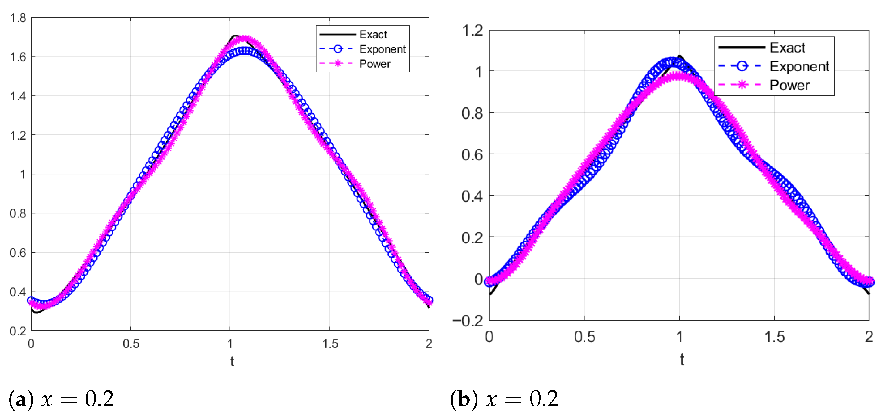
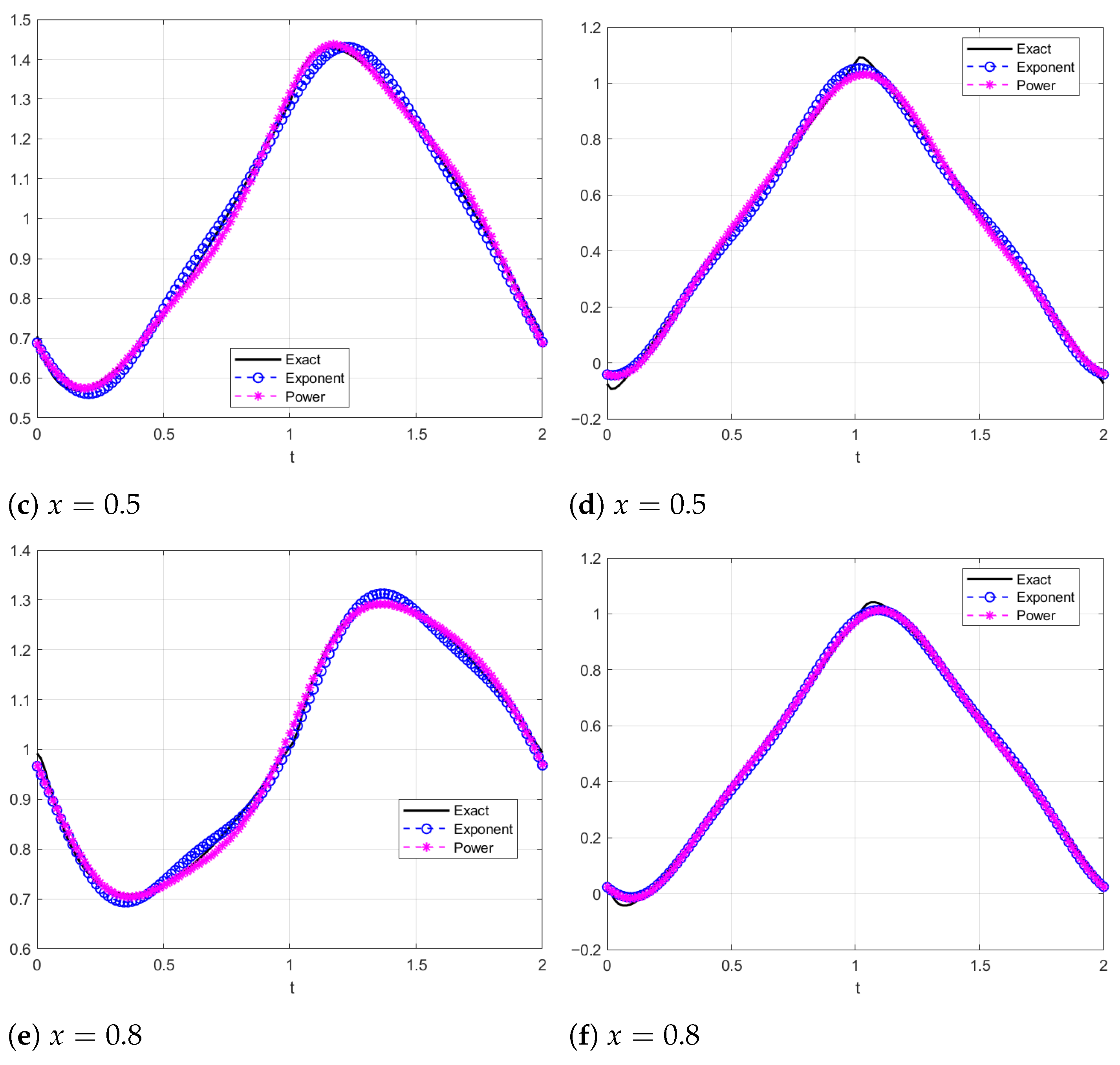
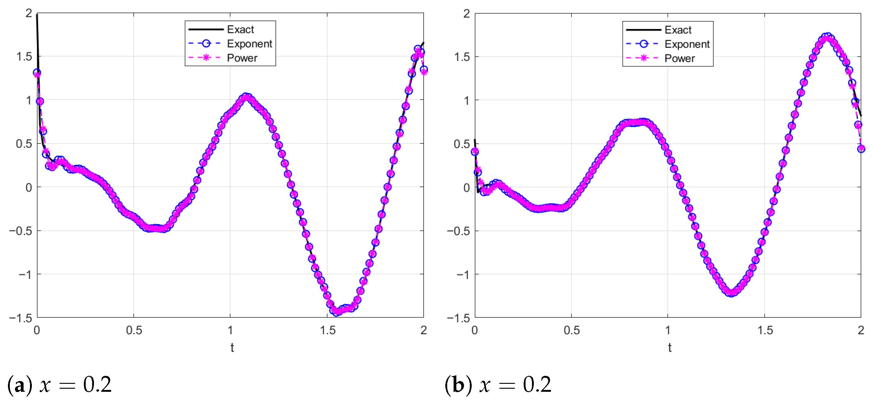
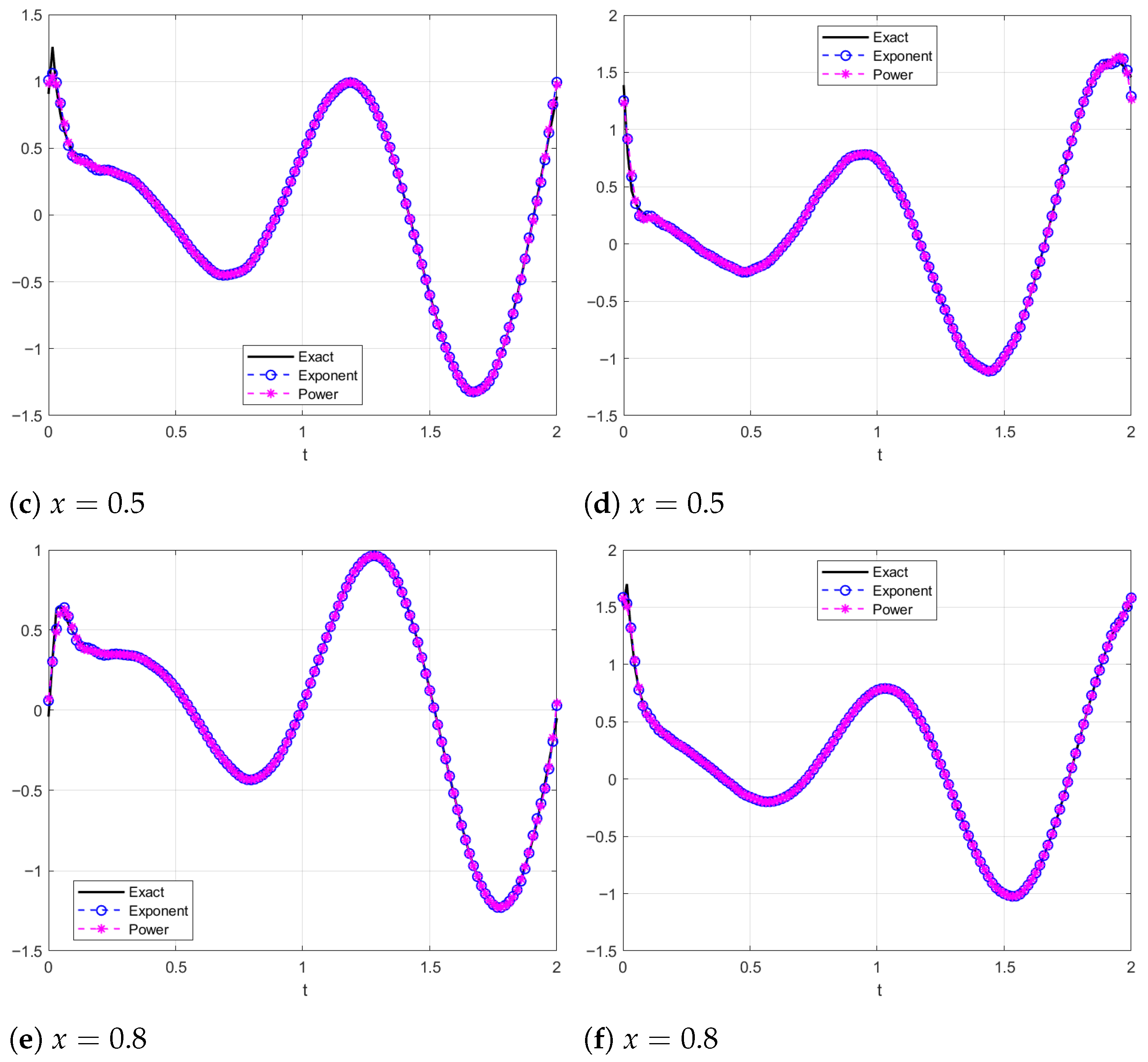
Table 1 and Table 2 show that for α = 0.2 and a priori choice of the regularization parameter, the relative errors of the regularized solutions obtained using the Dirichlet, Poussin, Exponent, and Power truncated kernels are identical. The reason is that, when α = 0.2, the a priori regularization parameter is sufficiently small such that the truncation threshold 1/μ exceeds the upper bound of the effective frequency range considered in our numerical experiments. Consequently, ${\widehat{P}}_{\mu }(\gamma )=1$ holds uniformly for all admissible frequencies, rendering the Dirichlet, Poussin, Exponential, and Power kernels numerically equivalent to the unit kernel. As a result, their corresponding regularized solutions—and hence the relative errors—coincide. Similar patterns are observed in Table 3 and Table 4. Consequently, all subsequent experiments adopt the a posteriori parameter selection strategy. For α = 0.8 and ϵ = 0.01, Figure 1 and Figure 2 display the exact solution and the regularized solutions obtained with different truncated kernels at several values of x. The figures show that these regularized solutions closely approximate the exact solution throughout the considered range of x.

Example 2.

We take the initial-value function.

$$w(t)=\left\{\begin{array}{cc}(1+i)t,\hfill & 0\le t\le 1,\hfill \\ (1+i)(2-t),\hfill & 1<t\le 2.\hfill \end{array}\right.$$

As in the first example, all results in

Table 5. Relative errors of the regularized solutions obtained with various truncated kernels for ϵ = 1.

		Real Part			Imaginary Part
	x	0.2	0.5	0.8	0.2	0.5	0.8
	α = 0.2	0.0777	0.0652	0.0525	0.1053	0.0781	0.0621
Dirichlet	α = 0.5	0.0794	0.0650	0.0528	0.1239	0.0828	0.0574
	α = 0.8	0.0872	0.0683	0.0560	0.1475	0.0907	0.0587
	α = 0.2	0.0543	0.0394	0.0290	0.0944	0.0834	0.0720
Poussin	α = 0.5	0.0572	0.0414	0.0322	0.0878	0.0705	0.0556
	α = 0.8	0.0720	0.0528	0.0434	0.1325	0.0838	0.0575
	α = 0.2	0.0654	0.0518	0.0397	0.0890	0.0726	0.0614
Exponent	α = 0.5	0.0684	0.0551	0.0453	0.0983	0.0821	0.0698
	α = 0.8	0.0736	0.0622	0.0542	0.0982	0.0753	0.0651
	α = 0.2	0.0525	0.0365	0.0238	0.0723	0.0676	0.0608
Power	α = 0.5	0.0567	0.0409	0.0306	0.0919	0.0689	0.0530
	α = 0.8	0.0775	0.0503	0.0351	0.1415	0.0694	0.0350

and

Table 6. Relative errors of the regularized solutions obtained with various truncated kernels for ϵ = 0.1.

		Real Part			Imaginary Part
	x	0.2	0.5	0.8	0.2	0.5	0.8
	α = 0.2	0.0220	0.0158	0.0110	0.0316	0.0276	0.0237
Dirichlet	α = 0.5	0.0209	0.0142	0.0109	0.0387	0.0281	0.0200
	α = 0.8	0.0254	0.0166	0.0137	0.0549	0.0371	0.0197
	α = 0.2	0.0170	0.0113	0.0107	0.0250	0.0227	0.0198
Poussin	α = 0.5	0.0190	0.0108	0.0104	0.0303	0.0260	0.0204
	α = 0.8	0.0210	0.0128	0.0106	0.0528	0.0261	0.0196
	α = 0.2	0.0196	0.0145	0.0104	0.0297	0.0250	0.0210
Exponent	α = 0.5	0.0254	0.0160	0.0105	0.0322	0.0274	0.0225
	α = 0.8	0.0267	0.0163	0.0126	0.0502	0.0304	0.0201
	α = 0.2	0.0184	0.0134	0.0094	0.0249	0.0219	0.0190
Power	α = 0.5	0.0181	0.0106	0.0104	0.0378	0.0300	0.0219
	α = 0.8	0.0203	0.0136	0.0122	0.0450	0.0285	0.0189

are obtained using the a posteriori parameter selection strategy, which has been shown to outperform the a priori strategy. The data consistently demonstrate that the a posteriori strategy yields stable and accurate reconstructions across various choices of ϵ, x, α, and truncated kernels.

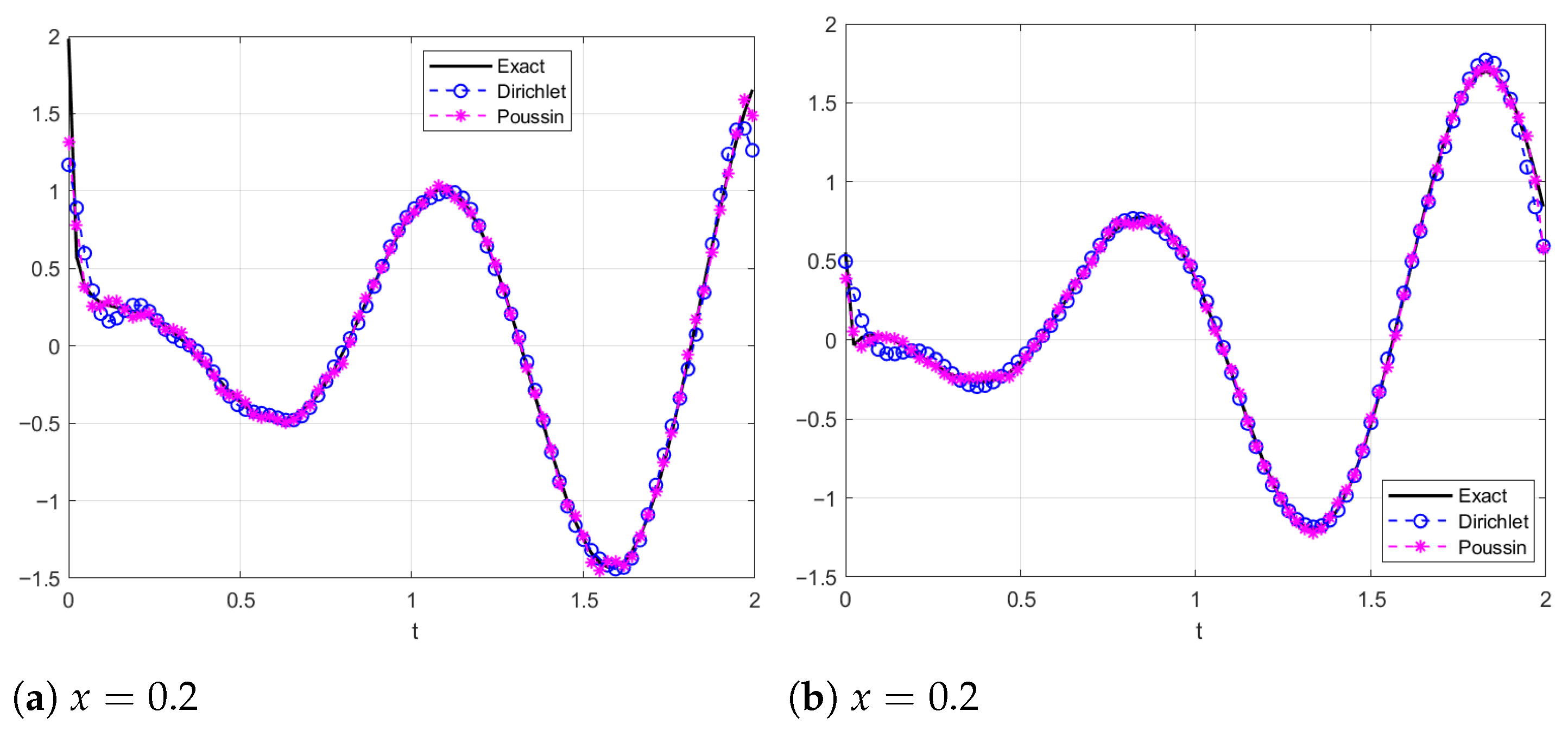
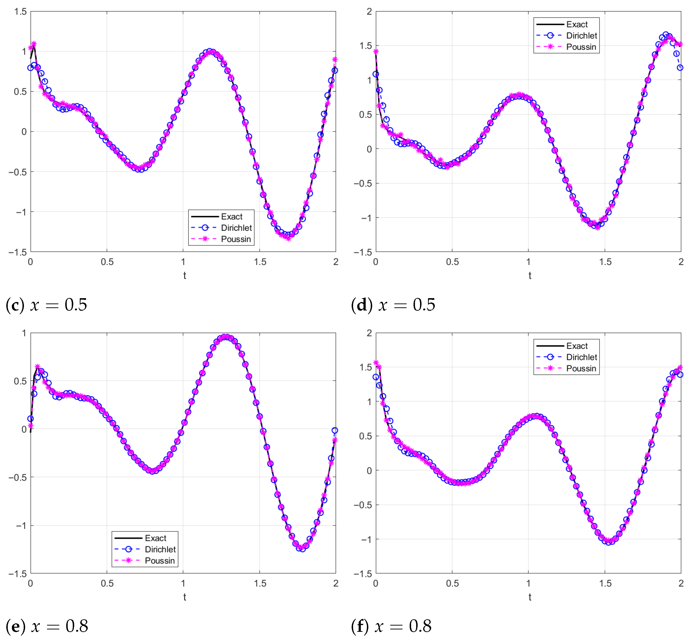
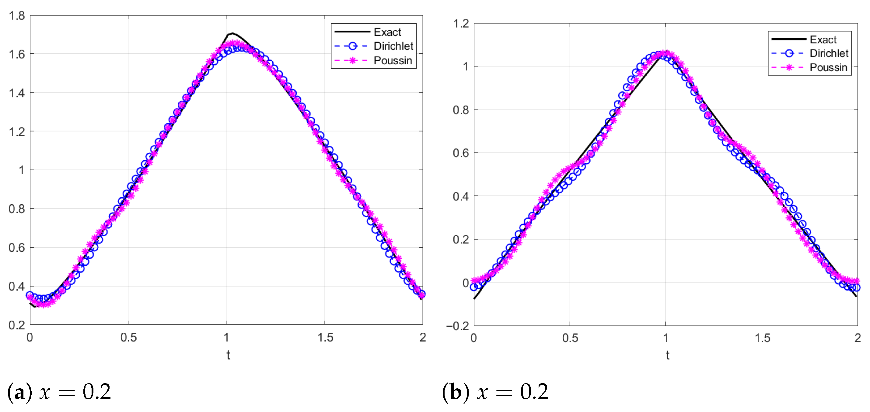
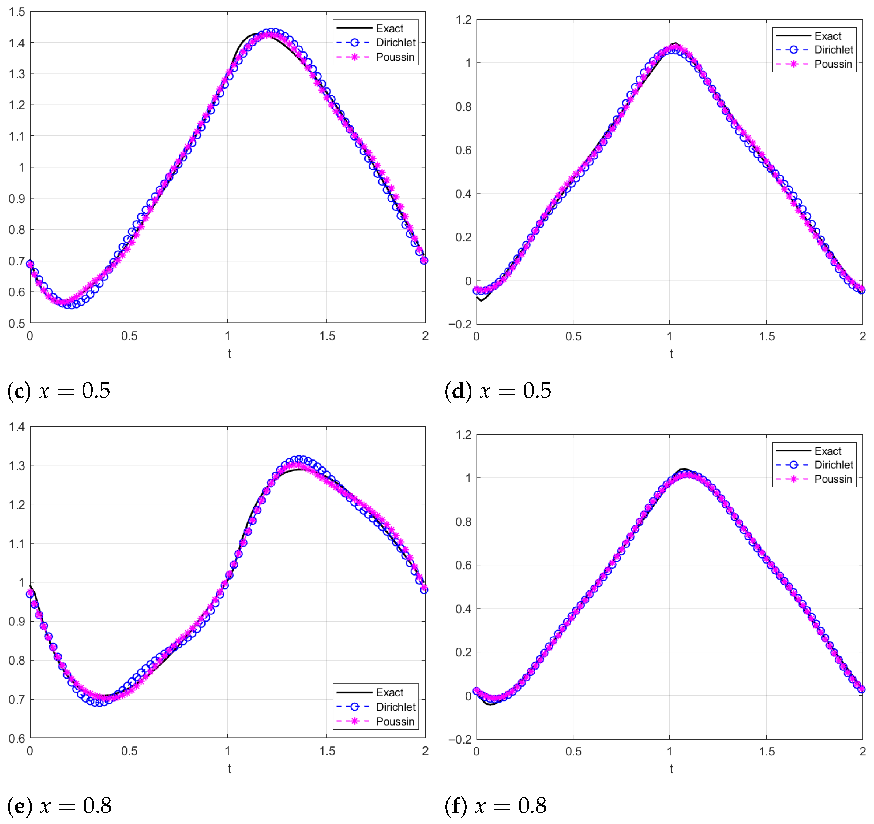
As shown in Table 5 and Table 6, the three-segment truncated kernel functions (Poussin, Exponential, and Power) consistently achieve superior results compared to the Dirichlet kernel. For instance, at x = 0.5, α = 0.5, in Table 5 (imaginary part), the Dirichlet kernel yields an error of 0.0828, while the Poussin, Exponent, and Power kernels achieve lower errors of 0.0705, 0.0821, and 0.0689, respectively. A comparison of Table 5 and Table 6 shows that reducing the noise level significantly decreases the relative errors for all methods. As the spatial depth x increases, the relative errors generally decrease for all kernels and noise levels. For instance, in Table 5 (Poussin, Real part, α = 0.5), the a posteriori error decreases gradually from 0.0572 at x = 0.2 to 0.0322 at x = 0.8. As the fractional derivative order α increases, the relative errors generally increase for most kernels and spatial depths x. For instance, in Table 6 (Poussin, Imaginary part, x = 0.5), the a posteriori error increases gradually from 0.0227 at α = 0.2 to 0.0261 at α = 0.8. These results are consistent with those observed in Example 1. For α = 0.8 and ϵ = 0.1, the exact solution together with the corresponding regularized solutions at various values of x are displayed in Figure 3 and Figure 4.

7. Discussion

Numerical experiments demonstrate that the regularized solutions obtained under both a priori and a posteriori parameter selection strategies are robust with respect to perturbed measurement data. A quantitative comparison of relative errors shows that the a posteriori strategy outperforms the a priori counterpart in terms of accuracy. Although theoretical error estimates show that the regularized solution achieves a higher convergence rate when the regularization parameter is chosen via the a priori strategy rather than the a posteriori one, this advantage relies heavily on a priori assumptions on the initial data. Such assumptions, however, are typically not accessible in practical computations, thereby rendering the theoretical convergence advantage unattainable in numerical experiments. Moreover, the three-segment truncated kernel yields superior regularization performance compared to the two-segment version. The experimental results also reveal a clear negative correlation between the degree of ill-posedness and the effectiveness of regularization: the weaker the ill-posedness, the higher the accuracy and robustness of the regularized solution.

8. Conclusions

This paper introduces a mollification regularization framework based on truncated kernels for solving the inverse time-fractional Schrödinger problem in a potential-free field. Both a priori and a posteriori strategies for selecting the regularization parameter are developed. Under suitable a priori assumptions on the initial data $u(0,·)$, error estimates for the regularized solutions are established for both parameter choice strategies. Theoretical analysis shows that the regularized solution achieves a faster convergence rate when the parameter is chosen via the a priori strategy rather than the a posteriori one, for both 0 < x < 1 and x = 0. Nevertheless, numerical experiments indicate that the a posteriori strategy yields more accurate regularized solutions in practice compared to the a priori approach. This occurs because the a priori strategy depends critically on the smoothness of the initial data—a condition rarely verifiable or achievable in practical computations.

References

1. Kenrow, J.A.; Gustafson, T.K. Schrödinger’s equation as a model approach to short time-scale quantum kinetics in a semiconductor. Phys. Rev. Lett. 1996, 77, 3605–3608. [Google Scholar] [CrossRef] [Scilit]
2. Sakhabutdinov, A.Z.; Anfinogentov, V.I.; Morozov, O.G.; Burdin, V.A.; Bourdine, A.V.; Gabdulkhakov, I.M.; Kuznetsov, A.A. Original solution of coupled nonlinear Schrödinger equations for simulation of ultrashort optical pulse propagation in a birefringent fiber. Fibers 2020, 8, 34. [Google Scholar] [CrossRef] [Scilit]
3. Ao, P.; Thouless, D.J.; Zhu, X.M. Nonlinear Schrödinger equation for superconductors. Mod. Phys. Lett. B 1995, 9, 755–761. [Google Scholar] [CrossRef] [Scilit]
4. Laskin, N. Fractional quantum mechanics. Phys. Rev. E 2000, 62, 3135–3145. [Google Scholar] [CrossRef] [Scilit] [PubMed]
5. Wang, S.W.; Xu, M.Y. Generalized fractional Schrödinger equation with space-time fractional derivatives. J. Math. Phys. 2007, 48, 043502. [Google Scholar] [CrossRef] [Scilit]
6. Zu, C.J.; Yu, X.Y. Memory effect in time fractional Schrödinger equation. Chin. Phys. B 2024, 33, 020501. [Google Scholar] [CrossRef] [Scilit]
7. Garrappa, R.; Moret, I.; Popolizio, M. Solving the time-fractional Schrödinger equation by Krylov projection methods. J. Comput. Phys. 2015, 293, 115–134. [Google Scholar] [CrossRef] [Scilit]
8. Köse, G.E.; Oruç, Ö.; Esen, A. An application of Chebyshev wavelet method for the nonlinear time fractional Schrödinger equation. Math. Methods Appl. Sci. 2022, 45, 6635–6649. [Google Scholar] [CrossRef] [Scilit]
9. Hicdurmaz, B. Finite difference schemes for time-fractional Schrödinger equations via fractional linear multistep method. Int. J. Comput. Math. 2021, 98, 1561–1573. [Google Scholar] [CrossRef] [Scilit]
10. Li, M.; Huang, C.M.; Wang, P.D. Galerkin finite element method for nonlinear fractional Schrödinger equations. Numer. Algorithms 2017, 74, 499–525. [Google Scholar] [CrossRef] [Scilit]
11. Kutluay, S.; Yamurlu, N.M.; Karaka, A.S. A robust quintic Hermite collocation method for one-dimensional heat conduction equation. J. Math. Sci. Model. 2024, 7, 82–89. [Google Scholar] [CrossRef] [Scilit]
12. Liu, N.; Jiang, W. A numerical method for solving the time fractional Schrödinger equation. Adv. Comput. Math. 2018, 44, 1235–1248. [Google Scholar] [CrossRef] [Scilit]
13. Yang, L.; Zhu, L.; He, S.Q. A mollification regularization method with Dirichlet kernel to solve potential-free field inverse Schrödinger Cauchy problem. Int. J. Comput. Math. 2024, 101, 942–960. [Google Scholar] [CrossRef] [Scilit]
14. Lv, X.L.; Feng, X.F.; He, S.Q. A kind regularization method with Poisson kernel to solve Cauchy problem of Schrödinger equation. Int. J. Comput. Math. 2025, 102, 203–223. [Google Scholar] [CrossRef] [Scilit]
15. Yang, L.; Zhu, L.; He, S.Q.; Zhao, B.X. Regularization of the time-fractional order Schrödinger problem by using the mollification regularization method. Math. Methods Appl. Sci. 2025, 48, 6799–6817. [Google Scholar] [CrossRef] [Scilit]
16. Yang, F.; Fu, J.L.; Li, X.X. A potential-free field inverse time-fractional Schrödinger problem: Optimal error bound analysis and regularization method. Math. Methods Appl. Sci. 2021, 44, 1219–1251. [Google Scholar] [CrossRef] [Scilit]
17. Yang, F.; Fu, J.L.; Li, X.X. A potential-free field inverse Schrödinger problem: Optimal error bound analysis and regularization method. Inverse Probl. Sci. Eng. 2020, 28, 1209–1252. [Google Scholar] [CrossRef] [Scilit]
18. Gao, Y.X.; Li, D.G.; Yang, F.; Li, X.X. Fractional Landweber iterative regularization method for solving the inverse problem of time-fractional Schrödinger equation. Symmetry 2022, 14, 2010. [Google Scholar] [CrossRef] [Scilit]
19. Ashurov, R.; Shakarova, M. Time-dependent source identification problem for a fractional Schrödinger equation with the Riemann–Liouville derivative. Ukr. Math. J. 2023, 75, 997–1015. [Google Scholar] [CrossRef] [Scilit]
20. Lv, X.L.; Feng, X.F. A kind regularization method for solving Cauchy problem of the Schrödinger equation. J. Comput. Appl. Math. 2025, 457, 116206. [Google Scholar] [CrossRef] [Scilit]
21. Lee, W. A variational technique of mollification applied to backward heat conduction problems. Appl. Math. Comput. 2023, 449, 127917. [Google Scholar] [CrossRef] [Scilit]
22. Qiao, Y.; Xiong, X.T. A mollifier approach to the simultaneous identification of the unknown source and initial distribution in a space-fractional diffusion equation. Appl. Math. Comput. 2025, 489, 129175. [Google Scholar] [CrossRef] [Scilit]
23. Lv, X.L.; Feng, X.F. Numerical method for a Cauchy problem for multi-dimensional Helmholtz equation. Appl. Math. Sci. Eng. 2024, 32, 2321450. [Google Scholar] [CrossRef] [Scilit]
24. Maréchal, P.; Triki, F.; Lee, W. Regularization of the inverse Laplace transform by mollification. Inverse Probl. 2024, 40, 025010. [Google Scholar] [CrossRef] [Scilit]
25. Yang, L.; Zhu, L.; He, S.Q.; Feng, X.F.; Zhao, B.X. Solving two kinds of inverse source problems for the heat equations by a mollification regularization method with Dirichlet kernel. Math. Methods Appl. Sci. 2024, 47, 14024–14036. [Google Scholar] [CrossRef] [Scilit]
26. Qiao, Y.; Xiong, X.T.; Han, J.J. A variational approach to recover the unknown source and initial condition for a time-space fractional diffusion equation. J. Appl. Math. Comput. 2025, 71, 3445–3476. [Google Scholar] [CrossRef] [Scilit]
Figure 1. Real part (left) and imaginary part (right) of the exact solution and the regularized solutions obtained with the Dirichlet and Poussin truncated kernels for Example 1 at different x, with α = 0.8 and ϵ = 0.01.
Fractalfract 10 00191 g001aFractalfract 10 00191 g001b
Figure 2. Real part (left) and imaginary part (right) of the exact solution and the regularized solutions obtained with the Exponent and Power truncated kernels for Example 1 at different x, with α = 0.8 and ϵ = 0.01.
Fractalfract 10 00191 g002aFractalfract 10 00191 g002b
Figure 3. Real part (left) and imaginary part (right) of the exact solution and the regularized solutions obtained with the Dirichlet and Poussin truncated kernels for Example 2 at different x, with α = 0.8 and ϵ = 0.1.
Fractalfract 10 00191 g003aFractalfract 10 00191 g003b
Figure 4. Real part (left) and imaginary part (right) of the exact solution and the regularized solutions obtained with the Exponent and Power truncated kernels for Example 2 at different x, with α = 0.8 and ϵ = 0.1.
Fractalfract 10 00191 g004aFractalfract 10 00191 g004b