1. Introduction
Tunis exhibits a Mediterranean climate (Csa, Köppen–Geiger classification) with distinct seasonal patterns: dry conditions from June to August and precipitation concentrated during the cool season [
1,
2,
3]. The rainfall regime displays significant seasonal and interannual variability. Annual rainfall at Tunis-Manoubia (monitored since 1873) averages around 444 mm but is highly concentrated during the cold season (October to April), with virtually no rainfall in summer. This pronounced seasonal pattern is compounded by extreme interannual fluctuations, ranging from 210 mm (2001–2002) to 808 mm (1958–1959)—representing 400% variation—resulting in alternating severe droughts and devastating floods [
4]. Since 1900, Tunisia has experienced 20 droughts and 14 floods [
4], equating to approximately one extreme event every three years.
This extreme variability results from the interaction of atmospheric mechanisms across multiple scales. Synoptic-scale circulation is driven by Mediterranean depressions, meso-scale rainfall is influenced by orographic effects from the Tell Atlas, and intense short-duration storms are produced by local convective processes [
5,
6]. The December 2003 event exemplifies this complexity: 186 mm fell in 24 h, causing catastrophic urban flooding and significant socioeconomic damage. At finer temporal scales, rainfall is highly intermittent, with 98–99% of 5 min intervals recording zero precipitation, yet when rain occurs, intensities vary dramatically across scales.
This multiscale and highly intermittent rainfall regime presents major challenges for hydrological analysis and flood risk management. It therefore requires analytical frameworks capable of characterizing scale-dependent variability and extreme intermittency [
7].
Energy spectrum analysis reveals scale-invariant regimes in rainfall processes. Each regime is represented by a power-law segment of the spectrum. Spectral analysis, a standard technique for analyzing stochastic signals with nonlinear variability [
8], serves as a preliminary step in multifractal analysis by assessing scale invariance and identifying scaling regimes [
9,
10]. Multiple scaling regimes in rainfall were initially identified using power spectral analysis, which relies on second-order statistics.
Fraedrich and Larnder [
8] analyzed European continental rainfall at daily and 5 min intervals, identifying several scaling regimes: a climate variability regime over three years with a spectral exponent β ≈ 0.7; a “spectral plateau” between one month and three years with β ≈ 0 reflecting large-scale circulation variability; a transitional regime from three days to one month mixing the spectral plateau and frontal systems; and a sub-three-day regime dominated by frontal dynamics with β ≈ 0.5. The spectrum below 2.4 h is governed by convective systems. Olsson et al. [
11] attributed spectral breaks, particularly those around 40 to 50 min, to changes in temporal rainfall structure corresponding to the average rainfall event duration. Later, Olsson [
12,
13] observed a spectral break around 2.4 h, which was initially unexplained but suspected to be artificial due to instrumental limitations in detecting weak signals. Fabry [
14] studying even shorter scales in Florida and Colorado using acoustic (sonic gauge) measurements, found a power spectrum similar to that of Fraedrich and Larnder’s [
8].
However, spectral analysis, based solely on second-order statistics, overlooks higher-order statistical properties essential for understanding extreme rainfall events—a critical limitation for Tunis where extreme events (floods and droughts) represent a major socioeconomic concern. To address this, research over the past two decades has focused on the multifractal nature of rainfall, characterized by an infinite spectrum of fractal dimensions arising from stochastic multiplicative cascade processes [
8,
12,
15,
16,
17,
18,
19,
20,
21,
22,
23,
24,
25]. These multifractal models are particularly effective for capturing the complexity of rare events in rainfall data and provide the theoretical foundation for this study’s investigation of Tunis rainfall across multiple temporal scales.
Recent advances in cascade-based rainfall modeling have focused on improving temporal autocorrelation structure in disaggregation schemes, with micro-canonical cascade models showing promising results for preserving realistic rainfall intermittency patterns across scales [
26]. However, these approaches still face challenges when applied to highly intermittent semi-arid rainfall, where parameter estimation bias due to extreme zero-value prevalence (>99%) remains inadequately addressed.
Rainfall shows intermittent behavior with alternating rain and dry periods, influencing both multifractal [
20,
27] and monoscaling analyses [
8]. Traditional fractal dimension measures based solely on spatial or temporal occurrence cannot fully capture rainfall’s variable intensity. Instead, multifractal models better represent its hierarchical complexity and scaling behavior.
Fractal dimension estimates depend on the rainfall threshold defining rain occurrence [
28,
29]. Higher thresholds reduce both the rainfall support and its fractal dimension [
11,
29,
30]. Consequently, rainfall is best described as a multifractal field characterized by a spectrum of fractal dimensions rather than a single value [
31]. This multifractal nature replaces threshold concepts with scale-invariant singularities, whose statistical properties follow scaling laws reflecting rainfall’s complex variability.
This behavior aligns with cascade models that replicate mass and energy conservation and symmetries inherent in the nonlinear Navier–Stokes equations [
32,
33]. Building on this foundation, the Universal Multifractal (UM) model introduced by Schertzer and Lovejoy [
34] captures these complex scaling behaviors through three key parameters. This model serves as a universal attractor for multifractal cascades under broad conditions. The cascade component is defined by two of these parameters (C
1 and α detailed later), while the third parameter extends the model to accommodate non-conservative processes (H). This minimal parameter set efficiently characterizes the essential scaling and intermittency properties of multifractal fields and has become a standard framework in multifractal analysis.
- -
C1 is the mean intermittency co-dimension (C1 ≥ 0), which measures the clustering of the (average) intensity at smaller and smaller scales. C1 = 0 for a homogeneous field.
- -
α is the multifractality index (0 ≤ α ≤ 2), which measures the clustering variability with regards to the intensity level.
- -
H is the degree of non-conservation, which quantifies the deviation of a process from conservative behavior. It measures the scale dependency of the average field (H = 0 for a conservative field).
A conservative process is characterized by a scale-invariant mean intensity. In this case, ⟨ε
λ⟩ remains constant across resolutions λ [
34]. This key property of multiplicative cascade theory ensures that statistical moments follow power-law scaling without a systematic bias in the mean: K(1) = 0 in the moment scaling function (Equation (3)). In contrast, non-conservative processes (H ≠ 0) exhibit a scale-dependent mean ⟨ε
λ⟩ ∝ λ
H, necessitating fractional integration (via the FIF model) to recover the underlying conservative cascade [
19,
34]. In hydrological applications, conservative scaling implies preservation of total rainfall volume upon aggregation, whereas non-conservative scaling (typically H > 0) reflects an apparent increase in mean intensity at finer resolutions, often due to measurement integration effects or intermittency.
Recent reviews by Monjo and Meseguer-Ruiz Vahab and Sankaran [
35,
36] illustrate that the UM framework remains the standard for rainfall analysis. However, these syntheses still rely on foundational methods that fail to fully resolve the numerical instability caused by extreme intermittency. This gap was first highlighted by De Montera et al. [
37], who showed that numerous zero values biases parameter estimation. While subsequent efforts [
16,
25,
38] attempted to bypass this by using non-zero values or fractal dimensions of support, a unified empirical correction capable of recovering the true physical signal in semi-arid conditions—as proposed in this study—is still missing from the current literature.
Two modeling approaches [
39] are recognized: one views rainfall support (time or space where rainfall occurs) as a fractal set [
40,
41]; the other attributes zero rainfall values to a physical and instrumental thresholding mechanism [
37,
38] due to difficulty in measuring low precipitation rates, which causes several artificial scaling regimes in low-rainfall regions [
38,
39,
42,
43]. Existing approaches to handle intermittency bias face critical limitations for semi-arid climates: event-by-event analysis [
37] requires continuous rainfall sequences that are extremely rare in Tunis (only 5 events > 2 h 40 min over 2.5 years); semi-empirical corrections [
16] were validated for moderate intermittency (60–80% zeros) and exhibit numerical instability when applied to extreme intermittency (>98% zeros, yielding
≈ 0); and threshold-based methods [
42] either exclude >99% of data or provide no bias reduction. These limitations necessitate a novel approach that can utilize partially rainy sequences while maintaining statistical robustness under extreme intermittency conditions. Lovejoy et al. [
43] studied the effect of high thresholds in space, noting that they induce scale breaks and bias parameter estimates. Distinguishing between real dry periods and artificial intermittency due to detection thresholds is a fundamental challenge. Furthermore, uncertainties related to rainfall measurements by rain gauges persist [
44,
45].
Insights from the literature provide a critical foundation for evaluating the applicability of the UM model in rainfall studies, revealing both its strengths and limitations. Most authors (
Table 1) begin multifractal analysis by examining the power spectral density, which provides key information on the conservation properties of the rainfall process through the spectral slope β. It is well established that β is strongly linked to data resolution and the analyzed scale range. Specifically, when β < 1, the rainfall process is conservative, meaning variance does not diminish significantly with scale, typical of medium to low frequencies (scales above one hour) as reported by several authors [
8,
11,
12,
13,
17,
21,
46]. Conversely, β > 1 indicates a non-conservative process, where variance reduces at larger scales, characteristic of high-frequency or heavy rainfall events observed by Verrier et al. [
16] and De Montera et al. [
37]. These spectral slopes are valid within scale ranges often bounded by scaling breaks. A consistent scale break near two weeks (3 days [
13], 11 days [
12,
21], 16 days [
17,
19], 21 days [
46], and 1month [
8]) marks the “synoptic maximum” [
47], representing the boundary between meteorological and atmospheric variability and corresponding to planetary-scale atmospheric dynamics [
43,
46]. Larger atmospheric structures evolve more slowly and display longer lifetimes, and the position of this break varies with regional climate [
19]. Once the scale invariance nature is established, authors apply the UM model. For daily data [
12,
15,
16,
18,
19,
24], α ranges from 0.45 to 0.7 and C
1 from 0.3 to 0.7, consistent with a universal class of rainfall processes described as bounded log-Lévy with finite singularities [
48,
49]. However, higher resolution data or intense rainfall, measured by instruments such as Dual-Beam Spectropluviometer (DBS) with fine temporal granularity, yield α > 1 and lower C
1 (~0.1) reflecting unbounded singularities and a complex intermittent structure characterized by variable-length continuous rainfall sequences [
16,
37]. Radar analyses of intense weather systems [
25,
38] yield parameter estimates in similar ranges: Gires et al. [
25] obtained α = 0.82−1.16 and C
1 = 0.26–0.35 for Mediterranean convective systems using 15 min radar data, while Verrier et al. [
38] reported α ≈ 1.1 and C
1 ≈ 0.17 for African monsoon rainfall from high-resolution radar observations. These radar-derived α values span the transition between bounded (α < 1) and unbounded (α > 1) multifractal regimes, with the higher end (α > 1) indicating complex intermittent structure with strong singularities characteristic of intense convective events. The relatively low C
1 values (<0.35) across both radar studies are consistent with the reduced intermittency observed at fine temporal resolutions (<1 h) for intense rainfall, supporting the instrument-independent nature of multifractal scaling at sub-hourly scales.
Parameter variability mainly arises from measurement resolution, rainfall intensity, and the intrinsic codimension of the rainfall support. For instance, a coarser temporal resolution typically leads to an overestimation of C
1 due to the averaging of extreme peaks, while higher rainfall intensities in convective events naturally result in higher C
1 values compared to stratiform events. Bias correction procedures [
20] can significantly adjust α and C
1 values—for example, correcting values from 0.75 and 0.45 to 1.55 and 0.05—indicating more complex, unbounded multifractal processes. Verrier et al. [
16] similarly showed that correcting biases shifts α and C
1 to 1.22 and 0.16, respectively, and delays the scaling break from three days to one week, confirming the necessity of bias treatment for accurate multifractal characterization. This synthesis elucidates the interplay between scale, instrumentation, and regional climatic context in determining multifractal properties of rainfall.
This study addresses two primary research questions for Tunis rainfall. First, what are the scaling properties of rainfall in a semi-arid Mediterranean climate? Specifically, we aim to identify distinct scaling regimes across temporal scales from 5 min to 2.5 years, determine the scale breaks separating these regimes, characterize each regime’s conservation properties through the H parameter, and estimate Universal Multifractal (UM) parameters (C
1, α) for each regime. This addresses a knowledge gap, as most existing studies focus on temperate or tropical regions (
Table 1), while semi-arid Mediterranean climates remain poorly characterized at high temporal resolution. Second, how can UM parameters bereliably estimated under extreme intermittency conditions? With more than 98% zero values in our dataset—compared to 60–80% in temperate regions [
16]—standard estimation methods yield significant bias, overestimating C
1 and underestimating α [
37]. Event-by-event analysis is impractical: only five continuous events longer than 2 h 40 min were observed over 2.5 years. We therefore develop an empirical bias correction method that explicitly relates the percentage of zero values to biased UM parameters, enabling parameter estimation from sequences with as few as 50% rainy observations (versus 100% required traditionally). This research provides (1) the first high-resolution (5 min) multifractal characterization of semi-arid Mediterranean rainfall; (2) practical bias correction methods applicable to data-scarce regions; and (3) a test of UM parameter universality across climatic zones. These advances improve our understanding of scale-dependent rainfall mechanisms. They also support hydrological modeling and flood risk assessment in semi-arid environments.
The structure of this paper is organized as follows:
Section 2 details the theoretical framework, focusing on the UM model and the associated multifractal and spectral analysis methodologies.
Section 3 describes the rainfall datasets and instrumental configuration.
Section 4 presents the results: it identifies scaling regimes, estimates fractional integration parameters (H) from spectral analysis, conducts structure function analyses, and derives UM model parameters α and C
1 for micro- and meso-scale regimes.
Section 4 also introduces an empirical bias correction method to address extreme intermittency, detailing its principles and applications at different temporal scales. Finally,
Section 5 summarizes our conclusions and future research perspectives.
2. Methodology
The rainfall field at temporal resolution λ (=T/t) is denoted ε
λ. It is defined as the ratio between the outer scaleTand the observation scalet. Numerically, the field ε
λ at various resolutions λ is obtained by successively degrading the initial measured field ε
Λ (Λ initial resolution), each step halving the resolution. Resolution degradation involves averaging finer-scale values to obtain coarser-scale ones, including in one-dimensional temporal fields. This aggregation process has two important statistical consequences for rainfall data: (1) Variance reduction: According to the Central Limit Theorem, averaging N independent values reduces variance by a factor of N, but for multifractal fields with scale-dependent correlations, variance follows a power-law decay
λ ∝ λ
K(2) (Equation (1) with q = 2), where K(2) characterizes the intermittency structure [
34]. (2) Intermittency evolution: The percentage of zero values decreases systematically with coarser resolution—for Tunis data, zeros represent 98.9% at 5 min resolution but only ~75% at daily resolution—as averaging increasingly combines rainy and non-rainy periods. The moment scaling function K(q) precisely characterizes these scale-dependent statistical transformations. (3) Statistical dependence: While fine-scale rainfall exhibits strong temporal correlations within events, aggregation to coarser scales progressively mixes independent rainfall systems, reducing dependence. These scale-dependent statistical transformations are precisely what multifractal analysis characterizes through the moment scaling function K(q), enabling reconstruction of fine-scale statistics from coarse-scale observations, and vice versa [
15]. The statistical characterization of ε
λ at different λ is commonly performed using its q-order statistical moments. For a multifractal field, these moments obey scaling laws:
The function K(q), representing the scaling behavior of the moments, exhibits convexity. As demonstrated by Schertzer and Lovejoy [
34], there exists an equivalent relationship linking the exceedance probabilities derived from an arbitrary singularity γ, expressed by the following equation:
The function c(γ), which defines the co-dimension, is an increasing and convex function. When c(γ) < d (d is the dimension of the field under study, which in this study is d = 1.), it can be interpreted as the fractal co-dimension of the support where the divergence, as λ→∞, of the field’s amplitude grows faster than λ
γ. The functions K(q) and c(γ) are related through the Legendre transform [
51]. These functions describe the variability of the studied field across scales and, in the most general case, depend on an infinite set of parameters.
The analytical expression of K(q) in this framework is given by the following equation:
For a conservative field: , i.e., K(1) = 0.
Take note that α = 0 for a process monofractal (β model). The case in which α = 2 corresponds to the maximum multifractality for a log-normal model.
These equations produce more mathematical definition for UM parameters (for more details, see Verrier et al. [
16]):
where K′ and K′′ are the first and second derivatives of K(q), respectively. For estimating the parameters of the UM model, more precise techniques exist, such as the Double Trace Moment (DTM) method introduced by Lavallée et al. [
52] and its modified version by Veneziano and Furcolo [
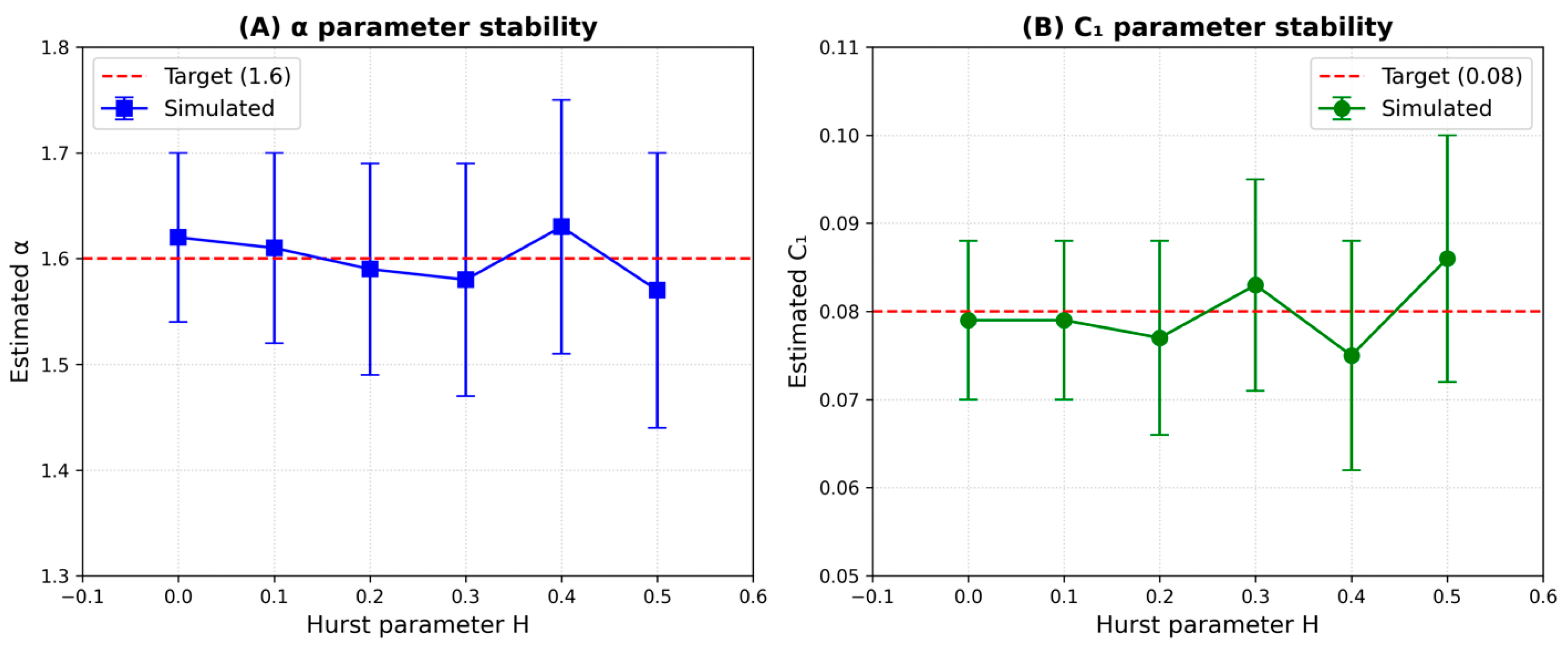
53]. To validate this approach for non-conservative processes (H > 0), we performed simulation tests (
Figure 1,
Table 2). We generated 300 synthetic Fractionally Integrated Flux (FIF) series with known parameters (α_true = 1.6, C
1_true = 0.08) across six levels of non-conservativity (H = 0, 0.1, 0.2, 0.3, 0.4, 0.5). For each series, we applied Equations (4) and (5) to estimate α and C
1 from the moment scaling function K(q). Results demonstrate robust parameter retrieval: mean errors remain below 2% for α and 4% for C
1 acrossall H values, including strongly non-conservative regimes (H = 0.5). Estimated parameters fall within ±10% tolerance for α and ±15% for C
1 (
Figure 1), confirming that direct application of Equations (4) and (5) correctly retrieves multifractal parameters even when H > 0. This validates our methodological choice for Tunis micro-scale rainfall (H = 0.14), where non-conservativity necessitates FIF modeling but does not invalidate moment-based parameter estimation.
Lastly, it is important to emphasize that the standard framework denoted
(i.e., where
) indicates a non-conservative field. Then,
can be written as (with equality in a probability distribution):
where ε
λ is a conservative field (
) of moment scaling function
.
depends only on UM parameters C and α. H characterizes the scale dependence of the average field:
H is equal to zero for a conservative field. The moment scaling function K(q) of
is given by:
where
is the moment scaling function of the non-conservative.
A field characterized by scale invariance fits an energy spectrum E(f), which is a representation of the characteristics of order 2 of the series in the frequency space, and follows a power law over a wide range of wave numbers f, where β is the spectral exponent, which is the negative slope of S(f) in a log–log graph [
8,
15,
54,
55]:
For multifractal fields, ref. [
56] shows that Equation (8) can be deduced from Equation (6) in the case of q = 2. According to the Wiener–Khintchine theorem, the slope of the power spectrum equal to β is related to the multifractal parameters through the following equation:
Spectral analysis estimates the parameter H, which quantifies non-conservative behavior in multifractal fields. For geophysical processes with spectral slopes β > 1, the Equation (10) links the spectral exponent to H and the intermittency parameter K(2). Fractional integration of order−H transforms the non-conservative field into a conservative one by removing the systematic scale-dependent trend in mean intensity.
As λ = T/Δt, considering q = 1 (first-order moment corresponding to mean flux), Equation (6) becomes:
f(Δt) is the first order structure function, when plotting it in log–log coordinates, the slope directly yields H.
When a strictly positive value of H is estimated, the rainfall time series must be differentiated and the corresponding conservative Fractionally Integrated Flux (FIF) process Φλ of order H can be reconstructed at lower resolutions by successively averaging pairs of contiguous values.
Empirical rainfall intensities often exhibit non-conservative behavior, where the mean intensity varies with scale as Rλ ∝ λH with H ≠ 0. Unlike ideal multiplicative cascades where statistical moments remain scale-invariant, non-conservative processes show systematic growth (H > 0) or decay (H < 0) of moments with scale, preventing direct multifractal analysis.
The Fractionally Integrated Flux (FIF) framework addresses this issue by treating the rainfall rate Rλ as the fractional integral of order H of a strictly conservative flux Φλ. This underlying flux satisfies Φλ = constant across all scales and can be recovered through fractional differentiation of the observed rainfall field. Once extracted, Φλ can be analyzed using the standard Universal Multifractal (UM) framework to estimate the intrinsic cascade parameters α and C1.
For discrete time series at resolution Δt, when H > 0 is detected, the fractional differentiation is applied to recover the conservative flux. The coarse-grained process at resolution λ × Δt is then reconstructed by successively averaging pairs of contiguous values, preserving the multifractal cascade structure while the H parameter accounts for the scale-dependent mean behavior.
3. Data Sets
The data used in this study were provided by the General Directorate of Water Resources (DGRE), Ministry of Agriculture of Tunisia. The study focuses on the Grand Tunis metropolitan region, comprising four governorates (Tunis, Ariana, Ben Arous, and Manouba). Three strategically positioned SYCOTRAC network stations provide representative spatial coverage: Tunis-Manoubia (Tunis Governorate) serves as the central urban reference, Sidi Thabet (Ariana Governorate) monitors the northwestern part, and Mornag (Ben Arous Governorate) provides data for the southeastern plains (
Table 3).
The SYCOTRAC system is a real-time hydrological measurement and flood warning network implemented after major floods in 2002–2003 damaged the Medjerda hydrometric infrastructure. All stations are equipped with automatic tipping-bucket rain gauges with 0.1 mm resolution per tip, recording at 5 min intervals. The analyzed dataset spans January 2008 to summer 2010 (2.5 years). This high-resolution dataset, while offering excellent temporal detail, is subject to specific measurement limitations that must be addressed in multifractal analysis:
Quantization effects: The discrete 0.1 mm resolution introduces specific challenges for multifractal analysis of differentiated series (required for non-conservative processes with H > 0, as discussed in
Section 4.1). At 5 min temporal resolution, a single tip corresponds to a constant intensity of 1.2 mm/h. When consecutive 5 min periods record identical low amounts (e.g., 0.1 mm, 0.1 mm), differentiation yields spurious zeros (0.1 − 0.1 = 0) despite continuous rainfall, artificially inflating the already high natural intermittency (98–99%) and introducing bias in Universal Multifractal parameter estimation. At rainfall rates below 2–3 mm/h, the 0.1 mm resolution cannot resolve intensity fluctuations smaller than 1.2 mm/h steps, effectively discretizing a continuous field and potentially affecting estimation of the multifractality index α at the finest scales. Quantization effects may create spurious spectral features or artificial scaling breaks reflecting measurement limitations rather than physical regime transitions. We address these effects through three complementary approaches: (1) when analyzing differentiated series, we exclude the finest 5 min scale and begin at 10 min where quantization represents a smaller fraction of the signal; (2) the bias correction procedure (
Section 4.4) applies a minimum intensity threshold (H
max> 1 mm/5 min = 12 mm/h), selecting only sequences where quantization effects are negligible relative to signal magnitude; (3) we validate corrected parameters against rare continuous high-intensity events where quantization represents <5% of measured values. These mitigation strategies, combined with the observation that most significant rainfall events in Tunis exceed 5 mm/h, confirm that 0.1 mm resolution adequately characterizes the dominant multifractal properties of the regional rainfall regime.
Tipping-bucket measurement uncertainties: Several systematic uncertainties affect tipping-bucket measurements in intensity-dependent ways. Wetting loss—water adhering to funnel and bucket walls—causes systematic underestimation of 0.1–0.3 mm per event and approximately 0.1 mm per tip [
45,
57], contributing 1–5% relative error for light rainfall (<2 mm/5 min) but becoming negligible (<1%) for moderate to heavy events (>5 mm/5 min). Mechanical undercatch at high intensities occurs because finite tipping time (~0.45–0.53 s) creates collection gaps; laboratory calibrations show 5–10% underestimation at intensities >50 mm/h, increasing to 13–20% at extreme rates (>200 mm/h) [
57,
58]. Conversely, slight overestimation (~2–5%) occurs at low intensities (<25 mm/h) due to incomplete drainage between tips. Wind-induced undercatch increases by approximately 1–2% per mph of wind speed for unshielded gauges [
59,
60], though this is partially mitigated for the relatively sheltered SYCOTRAC locations. Evaporation losses typically contribute <1–2% error for sub-daily measurements in Mediterranean climates. Complete or partial gauge blockage, while potentially causing measurement errors approaching 100% [
45], is rare in well-maintained operational networks (estimated frequency <0.1% for SYCOTRAC stations). Critically, such sporadic failures have limited impact on multifractal scaling analysis because Universal Multifractal parameters (C
1, α, H) are estimated from ensemble statistics—the scaling behavior of q-order moments <ε
qλ> averaged over thousands of data points at each resolution λ—making them robust to isolated errors representing <1% of data. For dominant Tunis rainfall patterns (5–50 mm/h), total measurement uncertainty is estimated at 5–15%, increasing to 15–25% for extreme events (>100 mm/h). These error ranges are acceptable for multifractal analysis, which characterizes statistical scaling properties through moment ratios and exponents rather than absolute rainfall amounts. Our analysis incorporates three quality control safeguards: visual inspection identifies suspicious periods with anomalously long zero sequences inconsistent with meteorological conditions; the bias correction procedure (
Section 4.4) naturally excludes low-quality periods likely affected by partial blockage through intensity thresholding; and multiscale validation comparing parameters estimated at different temporal resolutions (5 min differentiated series vs. 2 h 40 min aggregated series) and across methods (spectral vs. moment scaling) confirms consistency, indicating that instrumental limitations do not fundamentally compromise characterization of rainfall’s multifractal properties in the Tunis region.
Data transmission is performed using a data acquisition system that transmits tipping-bucket impulses via GSM modem to the receiving station located at DGRE. In case of failure, the network SYCOTRAC can be managed remotely.
There is a detailed statistical analysis of these data in ref. [
7]. This analysis shows that rainfall extends over nine months between September and May in a limited number of days, and they are practically null during the summer months (June, July, August). There is a pronounced maximum rainfall in December and no rainfall in July. According to that study, which aims to analyze the fractal dimension of rainfall support
Dfs (which characterizes the sparseness of the rain occurrences within the time series) using box-counting method [
28], three scaling regimes were identified: micro-scales [5 min–2 days], meso-scales [2 days–1 week], and synoptic scales [one week–8 months] with fractal dimensions
Dfs, respectively, around 0.44, 0.5,and 0.9. The study of rain support with intensity greater than 0.3 mm/5 min shows an extra break at 1 h 20 min. The additional break reflects a sub-regime of highly heterogeneous convective structures between 5 min and 1 h 20 min. This study highlights the extended duration of the saturation regime, confirming the relative homogeneity of rainfall support throughout the year. Unlike less variable climates, precipitation here is not consistently observed over one- or two-week periods; instead, rain occurs at least once every 113 days or more.
4. Results and Discussion
4.1. Determination of Scaling Regimes, and Non-Conservation Factor
Before presenting our analyses, we articulate four testable hypotheses that guide this study:
- -
H1: Tunis rainfall exhibits at least three distinct scaling regimes (micro-, meso-, synoptic) with different physical mechanisms, similar to temperate climates [
8].
- -
H2: High-frequency rainfall (<3 h) exhibits non-conservative behavior (β > 1, H > 0) driven by convective processes, consistent with findings in temperate regions [
16,
37].
- -
H3: Standard UM parameter estimation significantly underestimates α and overestimates C1 when applied to data with >95% zeros, requiring correction methods that account for rainfall support fractal dimension.
- -
H4: After bias correction, UM parameters for Tunis align with the universal class of rainfall processes (bounded log-Lévy: 0.5 < α < 0.7, 0.3 < C1< 0.7 for daily data; α > 1, C1 ≈ 0.1 for high-resolution continuous events), despite climatic differences.
The following subsections test these hypotheses systematically.
4.1.1. Identification of Scaling Regime Through Convergent Criteria
Robust regime identification requires convergence of multiple independent criteria to avoid arbitrary break placement and associated parameter bias. We employed three complementary criteria:
- -
Criterion A (Spectral analysis) reveals distinct linear segments in log E(ω) vs. log ω with R2 > 0.85. Clear scale breaks are observed at 2 h 30 min (where β shifts from 1.14 to 0.42) and at 7 days (β dropping to 0.09).
- -
Criterion B (Structure function analysis) independently confirms the micro-to meso-scale transition. This analysis shows a sharp transition in the Hurst parameter, moving from H = 0.14 for scales δt < 2 h 30 min to a near-zero value (H ≈ 0) beyond this threshold.
- -
Criterion C (Moment scaling validation) ensures scale invariance within each identified regime, maintaining R2 > 0.85 for log⟨ελq⟩ vs. log λ across all q ∈ [0, 2].
4.1.2. Application of Spectral Analysis
Spectral analysis of complete datasets from three stations spanning 2.5 years at 5 min time steps serves as a preliminary stage intended to identify different regimes of scale invariance and assess their conservative (or non-conservative) nature.Given the influence of zeros on the analysis results, we employ two complementary approaches: analysis of complete 2.5-year datasets and analysis restricted to wet periods beginning September 1st (excluding dry summer months). For the wet-period approach, series of approximately eight months (216 × 5 min) were selected when available, as the rainy season in Tunis begins in September with virtually no rainfall during summer.
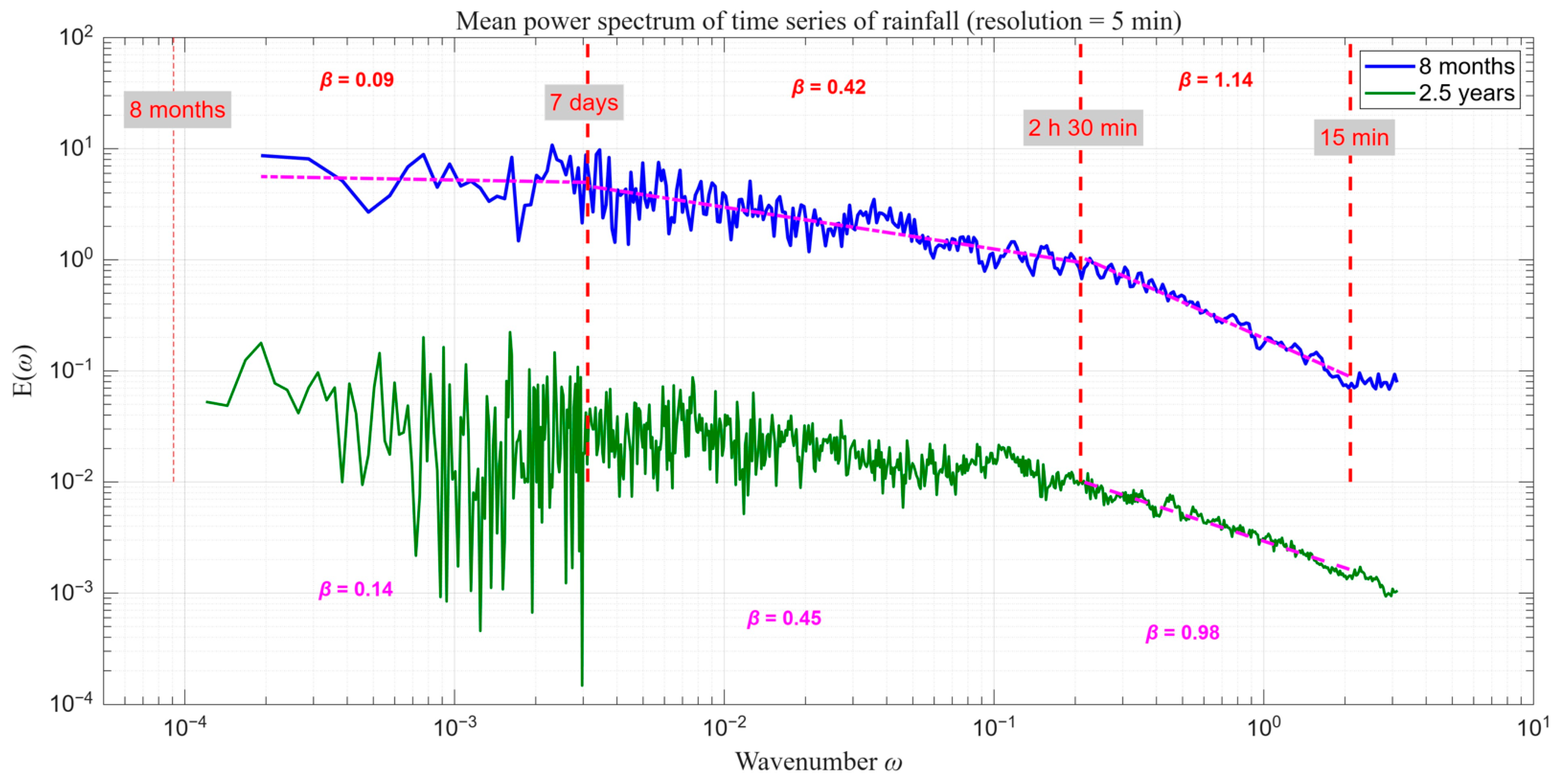
Even during wet periods, zero values remain highly prevalent (98.6% vs. 99.1% for complete series), explaining the similarity of results between both approaches. Average spectra were computed for both the 2.5-year and 8-month series (
Figure 2). The
spectral exponent (of the spectrum), β (Equation (9)), was estimated for each scale range exhibiting scale invariance.
Table 4 summarizes the spectral analysis results.
Figure 2 reveals two scale breaks. The first break is located around 2.5 h and the second break at one week. These two breaks distinguish three regimes of scaling: micro-scale [5 min–2 h 30 min], the meso-scale [2 h 30 min–1 week], and synoptic scale [1 week–L_series]. The flattening behavior observed at the high-frequency end of the spectrum (time scales shorter than 15 min) is likely caused by quantization noise. This effect stems from the instrumental limits of the tipping-bucket rain gauge and the discrete nature of the measurements, which tend to mask the scaling at very fine scales.
The spectral slope β in the first regime for the 5 min resolution rainfall series is equal to or greater than 1, indicating a non-conservative process at high frequencies (micro-scale). However, rainfall becomes a conservative process at meso-scales with a spectral slope β less than 1 (range 0.4 to 0.7). Results for synoptic scales (7 days–2.5 years/8 months) are uncertain due to insufficient dataset length but values remain close to zero. The break atone week is also consistent with previous analyses using daily data (
Table 4, last line).
By comparing the spectra from the series length of 2.5 years and those of 8 months (
Figure 2), we notice that the values of the spectral slope β significantly increase for regime 1 corresponding to the high frequencies [(15 min)
−1–(2 h 30 min)
−1]. Station-specific analysis shows notable differences in micro-scale behavior. While Mornag and Sidi Thabet exhibit non-conservative processes (β > 1), Tunis-Manoubia displays conservative scaling (β
1 = 0.67). This heterogeneity explains the lower combined average (β
1 = 0.98) for the 2.5-year datasets compared to the 8-month series (β
1 = 1.14).
The break observed around 2 h 30 min (from 1 h to 3.5 h) is consistent with Fraedrich and Larnder [
8], which identified a break at 2.4 h. This scale could represent the boundary between convective and frontal systems, characterized by β > 1 as an indicator of non-conservative behavior. The positions of the first break as well as the value of the slope of the first regime differ significantly according to the analysis strategy employed. For series of eight months, which exclude the summer, the percentage of zeros is only slightly lower, but we observe that the first break seems to appear earlier (between 1 and 2.5 h) with a slope greater than 1 on average, whereas for the complete dataset the break is observed between 2 h 20 min and 3 h 30 min. The mean slope is 0.98.
The position and characteristics of the first break around 2 h 30 min warrant careful interpretation given the extreme intermittency (98–99% zeros) in our dataset. Three diagnostic tests support the hypothesis advanced by de Montera et al. [
30] that this break may reflect artificial effects from null values rather than purely physical regime transitions.
First, the break position is analysis-strategy dependent: for eight-month series excluding summer (98.6% zeros), the break appears earlier (1–2.5 h) with mean spectral slope β1 = 1.14, whereas for complete 2.5-year series (99.1% zeros), the break shifts to 2 h 20 min–3 h 30 min with β1 = 0.98. This sensitivity to zero-value percentage, where a marginal 0.5% increase in zeros produces a ~30–60 min shift in break position and 14% reduction in β1, suggests intermittency-related artifacts rather than a fixed physical scale.
Second, comparison with continuous rainfall events provides direct evidence: analysis of the five identified continuous events (>2 h 40 min duration, zero intermittency) yields no detectable spectral break in the 10 min–2 h 40 min range; instead, these events exhibit consistent power-law scaling with β = 1.55–1.77 across this entire range, characteristic of convective systems [
16]. The emergence of a break only when zeros are present—and its position correlating with zero percentage—directly implicates intermittency rather than atmospheric physics.
Third, the spectral slope below the break is unusually low for the intermittent series: β
1 = 0.98–1.14 in our analysis contrasts with β = 1.55–1.77 for continuous events and β > 1.5 reported in temperate climates [
16,
37]. This suppression of β
1 is consistent with theoretical predictions showing that intermittency biases spectral estimates toward lower values [
37]. It provides quantitative evidence that the observed break and associated slope do not purely reflect a physical transition from convective to frontal systems.
However, we emphasize that complete attribution to artifacts would be oversimplified: the 2–3 h timescale does align with typical convective cell lifetimes and the transition scale observed in other climates [
8], suggesting the observed break likely represents a combination of physical regime transition and intermittency-induced artifacts. Our bias correction methodology (
Section 4.4) addresses this ambiguity by analyzing sequences with reduced intermittency (50–90% zeros rather than >98%) and validating against continuous events, enabling reliable parameter estimation despite uncertainty in break interpretation. The corrected spectral slope (β = 1.13 from corrected UM parameters) closely matches the observed spectrum for wet periods (β = 1.14), supporting the effectiveness of our approach.
The second break, located at one week, is also consistent with previous studies, mainly using daily data, which found breaks close to our results despite the different resolutions (namely Olsson [
12], de Lima et Grasman [
21], Verrier et al. [
16] reporting breaks at =[11, 8, 7 days]).
For the third scaling regime, which is governed by large-scale atmospheric circulation, there is a spectral plateau with β roughly close to 0. This regime is mentioned in refs. [
8,
13], though with fairly different scale breaks.
4.2. Structure Function Calculation
Since the micro-scale regime shows a spectral slope β very close to 1, the upper limit indicative of a non-conservative process, and given that the limits of scaling regimes are subjective and depend on visual assessment, a study of the first-order structure function is necessary to infer more precisely the parameter H. This parameter quantifies the degree of non-conservation of the process. The structure function also enables more precise determination of when the phenomenon becomes conservative.
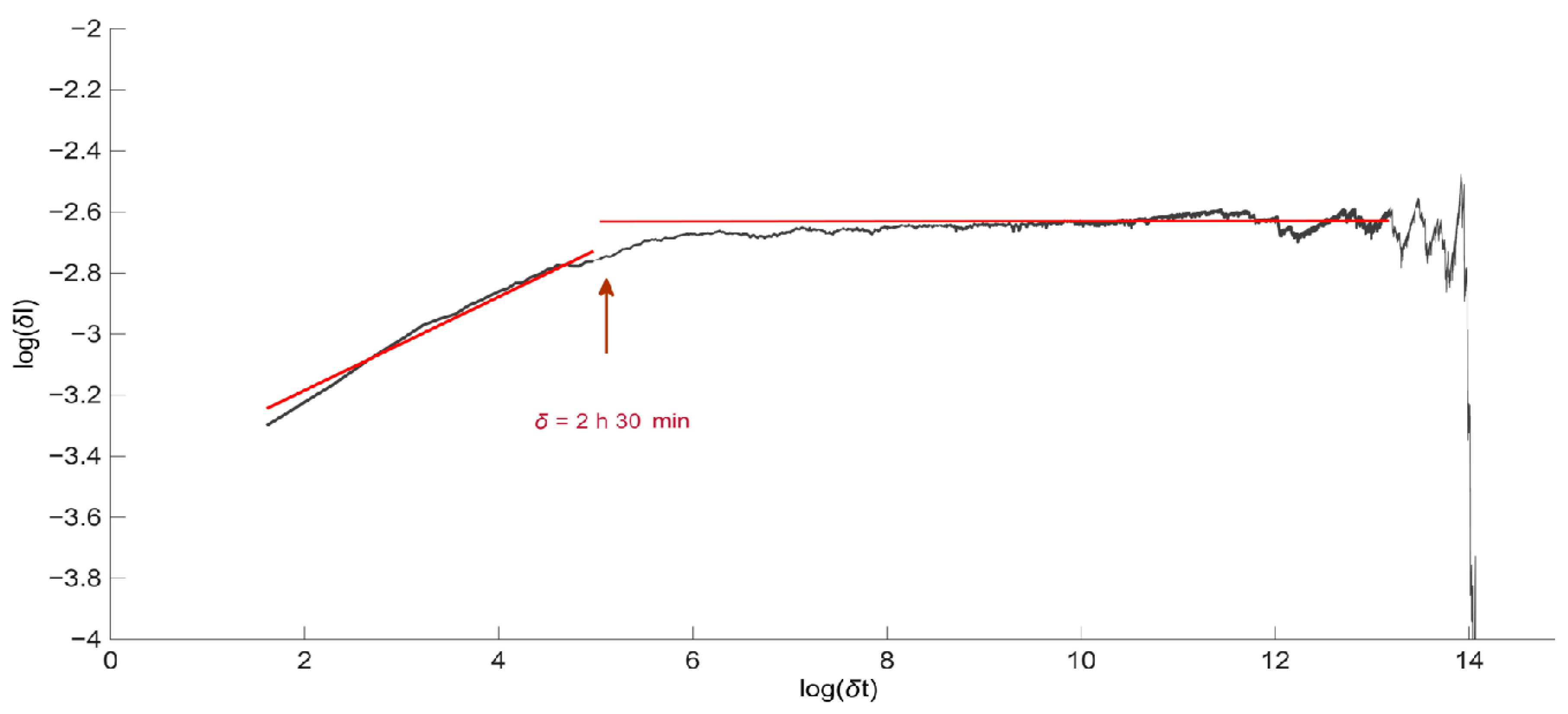
Results for the parameter H, which quantifies the process deviation from a conservative process, are illustrated in
Figure 3 in logarithmic coordinates. The slope of the curve corresponds to the exponent H (Equation (11)).
Figure 3 for Tunis-Manoubia shows the slope of log
versus log (δt) (H) rising until δt = 2 h 30 min, and then stabilizing near zero, indicating two regimes around this breakpoint. The high-frequency regime (δt < 2 h 30 min) is non-conservative with H > 0, implying the rain rate is not a pure multiplicative cascade but requires fractional integration to reconstruct it. The second regime (δt ≥ 2 h 30 min) is conservative (H ≈ 0). All three stations exhibit similar behavior (
Table 4, column 3), consistent with spectral rainfall analysis.
Spectral analysis reveals breaks at approximately 2 h 30 and one week. For multifractal analysis, the observed 2 h 30 min break was approximated by 2 h 40 min (corresponding to 25 × 5 min = 32 time steps), as the Universal Multifractal framework requires dyadic scale decomposition (powers of 2) for accurate parameter estimation. This 10 min adjustment (4% difference) ensures methodological rigor while remaining within the observed break’s uncertainty range (2 h–3 h).
These findings confirm micro-scale non-conservative behavior, as indicated by spectral slopes exceeding 1 and positive H values, consistent with previous studies [
8,
16,
37].
The rainfall process transitions to conservative behavior at meso-scales (2 h 40 min to 7 days) (
Table 5) are characterized by spectral slope β < 1 (range 0.4–0.7) and H ≈ 0. This transition reflects a fundamental change in dominant atmospheric mechanisms specific to the Tunis Mediterranean climate. This transition corresponds to the shift from convective-dominated to frontal-system-dominated precipitation generation.
At micro-scales (<3 h), rainfall in Tunis is primarily driven by localized convective cells—intense, short-lived storms with rapid vertical development and strong updrafts that generate highly variable rainfall intensities over small spatial and temporal scales. These convective systems exhibit non-conservative behavior (β > 1, H > 0) because mean rainfall intensity systematically increases with finer temporal resolution: as observation intervals shorten from hours to minutes, the measured intensity spikes during convective burst cores become increasingly prominent relative to the quiescent periods between cells, causing ⟨ελ⟩ ∝ λ−H with H > 0. This scale-dependent mean reflects the intermittent, “bursty” nature of convection where energy input (latent heat release) occurs in localized regions and times rather than being uniformly distributed.
In contrast, at meso-scales (hours to days), Tunis rainfall is increasingly influenced by synoptic-scale frontal systems—organized bands of precipitation associated with Mediterranean depressions that produce more spatially and temporally homogeneous rainfall distributions. Frontal precipitation results from large-scale atmospheric lifting along density boundaries, generating stratiform rain with relatively steady intensities over extended periods (6–24 h). For these systems, energy input (from large-scale baroclinic instability) is distributed more uniformly across the precipitation field, resulting in conservative flux behavior where mean intensity remains approximately constant across temporal scales (⟨ελ⟩ ≈ constant, H ≈ 0) and variance scales classically with resolution (β < 1). The observed spectral slopes (β = 0.4–0.7) align with values reported for frontal systems in other Mediterranean and temperate climates [
8,
21], confirming that meso-scale Tunis rainfall shares the conservative scaling properties characteristic of large-scale organized precipitation systems. The one-week upper boundary of this regime corresponds to the synoptic maximum—the typical lifetime of Mediterranean depression systems affecting Tunisia—beyond which inter-storm variability and seasonal climate fluctuations dominate.
This physical interpretation is consistent with the seasonal rainfall pattern in Tunis, where winter months (October–April) are characterized by successive frontal systems producing the majority of annual precipitation, while summer convection contributes minimal rainfall but with extreme intensity variability when present. The conservative meso-scale regime thus reflects the prevalence of organized frontal precipitation in the region’s dominant rainfall climatology.
These meso-scale spectral slopes are consistent with values reported across diverse climatic regions for frontal-dominated precipitation (0.2, 0.37, 0.4, 0.5, 0.41, and 0.66) for various Mediterranean and temperate locations [
8,
12,
16,
17,
19,
21], with the notable exception of Tokyo, where Pathirana et al. [
22] observed β > 1, likely reflecting stronger convective influence in East Asian monsoon systems. The identification of three distinct scaling regimes (micro-, meso-, synoptic) with breaks at approximately 2 h 30 min and one week is further supported by complementary analysis of rainfall occurrence using box-counting methods [
7], which independently identified the same three-regime structure with fractal dimensions of 0.44, 0.5, and 0.9, respectively, and a scale break at one week corresponding to the synoptic maximum. This multiple method consistency strengthens confidence that the observed regime transitions reflect genuine physical scale breaks in Tunis rainfall generation mechanisms. This remains true despite the complications introduced by the extreme intermittency discussed above.
4.3. Parameter Estimation for the U M Model
Since the rainfall process is non-conservative at fine scales, we employed two approaches to obtain K(q):
(i) The first approach applies the standard FIF model to the 5 min time step series. We follow the methodology described in ref. [
52], which consists of modeling the differentiated series:
. As a first step, we verify the validity of the two scaling regimes obtained by spectral analysis by assessing the linearity of the relationship between
and log λ for different values of q. Then, we estimate the parameters of the function K(q) by determining the different slopes of the linear relationship. The coefficients of determination for linear regressions are calculated and a test ensures that they exceed 0.85.
(ii) The second approach involves averaging the data set to a time step equal to 2 h 40 min: . According to the previous analysis, the resulting series corresponds to a conservative process and can be modeled using the UM framework. In this case we assess the linearity of the relationship between and log λ.
Given the extreme sensitivity of UM parameter estimates to intermittency levels, we employ two complementary analysis strategies. The first analyzes complete 2.5-year datasets (99.1% zeros, n = 218 × 5 min points per station), while the second restricts the analysis to eight-month wet seasons (September–April, 98.6% zeros, n = 216 × 5 min). This dual approach addresses potential sampling biases from seasonal heterogeneity. Summer months (June–August) contribute <1% of annual rainfall but represent ~25% of the temporal coverage, creating extended zero sequences that introduce three specific biases: (1) spurious zero inflation from climatological drought confounding intermittency-parameter relationships; (2) systematic suppression of micro-scale spectral slopes (β1 ≈ 0.98 for complete series versus 1.14 for wet-season series); and (3) amplification of meso-scale slopes (β2 ≈ 0.62 versus 0.42, +48% difference). Critically, while absolute slope values differ between approaches, the positions of spectral regime transitions remain consistent, and both strategies identify the same three distinct scaling regimes. This validates that our primary conclusions regarding scaling transitions are robust to seasonal sampling decisions rather than methodological artifacts.
UM parameters α and C1 are estimated from K(q) derivatives using Equations (4) and (5) (K′(1) = C1, K″(1) = α·C1), validated against least-squares fitting. The multifractality index α quantifies intensity variability (α > 1: unbounded fluctuations), C1 measures spatial–temporal clustering, and H characterizes scale-dependent mean evolution (H > 0: non-conservative).
Micro-scale UM parameter estimation, after bias correction described in
Section 4.4, yields α ≈ 1.6, C
1 ≈ 0.1, and H ≈ 0.14. The multifractality index α > 1 reflects unbounded intensity singularities characteristic of highly intermittent Mediterranean convective processes, where localized storm cells generate intense bursts separated by quiescent periods. The relatively low intermittency codimension (C
1 ≈ 0.15) compared to temperate climate values (0.3–0.7) [
16,
37] indicates that despite extreme occurrence intermittency (98% zeros), active rainfall events exhibit relatively uniform intensity distributions—a signature of Mediterranean convection where individual cells produce homogeneous precipitation within their spatial extent. The positive non-conservativity parameter (H ≈ 0.14) confirms “bursty” structure where short-duration intensity peaks dominate the statistical moments.
At meso-scales, parameters shift to α ≈ 0.6, C1 ≈ 0.2, and H ≈ 0, reflecting transition to conservative scaling dominated by organized frontal systems with bounded intensity structures typical of synoptic Mediterranean depressions. These multiscale parameter variations quantitatively characterize the physical rainfall generation mechanisms operating in Tunis’ semi-arid Mediterranean climate, enabling comparison with other climatic regions and validation of theoretical multifractal cascade models.
As in the previous section and given the sensitivity of the estimate to the presence of null values, the study is performed firstly by using datasets spanning two and a half years and secondly using the 8 months series excluding the dry period.
Once the experimental moment scaling function K(q) is obtained, the parameters α and
C1 are estimated using two methods: The first method, called the (i) optimization method, directly adjusts the theoretical form of the pairs (
q,
K(
q)) using a least-squares minimization approach. The properties of the moment scaling function permit a direct estimation of the parameters using the first and second derivatives of
K(
q). The latter was called the (ii) derivation method:
For simplicity reasons, the results obtained with both methods are presented only when they are significantly different.
As the results obtained with these different approaches (differentiated 5 min times series or averaged data up to the first break; 8 month rainfall series or full time rainfall series; optimization or derivation estimation method) are quite similar, for simplicityreasons, only parameters estimated with the differentiated full times series and optimization estimation method are presented in
Table 4.
4.3.1. Micro-Scale Analysis (5 min–2 h 40 min)
We obtain
C1 equal to 0.48 and α practically zero for micro-scales. The value of C
1 is close to previous studies, especially those for which the effect of intermittency was not considered. Concerning α, many authors [
20,
21,
37,
38,
49] have already pointed out the existence of a bias in the estimation of parameters for intermittent rainfall. However, the obtained zero value, characteristic of a monofractal process, is not obtained in previous work (
Table 1).
This anomalously low α value (≈0, characteristic of monofractal processes) contradicts physical expectations for convective rainfall and empirical observations from continuous events (
Section 4.3.1), indicating systematic bias in parameter estimation. Statistical analysis quantifies two contributing factors.
First, the extreme intermittency inherent to Tunis’ semi-arid Mediterranean climate produces 98.6–99.1% zero values in our 5 min resolution datasets (
Table 3), substantially higher than the 60–80% typical of temperate regions where UM parameter estimation methods were developed and validated [
16,
37]. Simulation studies by de Montera et al. [
37] demonstrate that α estimation systematically converges toward zero as intermittency exceeds 95%, precisely the regime encountered in Tunis data.
Second, data quantization from 0.1 mm tipping-bucket resolution artificially inflates zero counts in differentiated series used for micro-scale analysis. When consecutive 5 min periods record identical low rainfall amounts (e.g., 0.1 mm, 0.1 mm), differentiation yields artificial zeros (0.1 − 0.1 = 0 mm) despite continuous precipitation. To quantify this effect, we compared zero percentages between (a) original rainfall series: 98.9% zeros; (b) differentiated series for micro-scale analysis: 99.4% zeros—a 0.5 percentage point increase attributable to quantization. While this increment appears modest, it occurs precisely in the critical range (>98%) where UM parameter estimation is most sensitive to intermittency artifacts [
37]. Furthermore, analysis of intensity distributions shows that 45% of non-zero 5 min observations fall below 0.3 mm (corresponding to <3.6 mm/h), the range where quantization effects are most pronounced and differentiation most likely to introduce spurious zeros. The combined effect of climatological intermittency (98.9%) and quantization-induced zeros (+0.5%) produces the extreme intermittency (99.4%) that biases α toward zero. Validation through continuous-event analysis (
Section 4.3.1) confirms this interpretation: the five identified continuous rainfall sequences (zero intermittency by definition) yield physically realistic α values (1.3–1.4), demonstrating that bias arises from intermittency and quantization rather than fundamental rainfall physics in the Tunis region.
To overcome the errors introduced by the problems described above, a new analysis of the micro-scale regime was performed by selecting shorter series with no zeros. Given the necessary differentiation of the series for the study of this regime, the impact of data quantization is very important for low intensity events because it creates artificial zeros, which are added to existing zeros (no rain), thereby intensifying the problem of bias in parameter estimation.
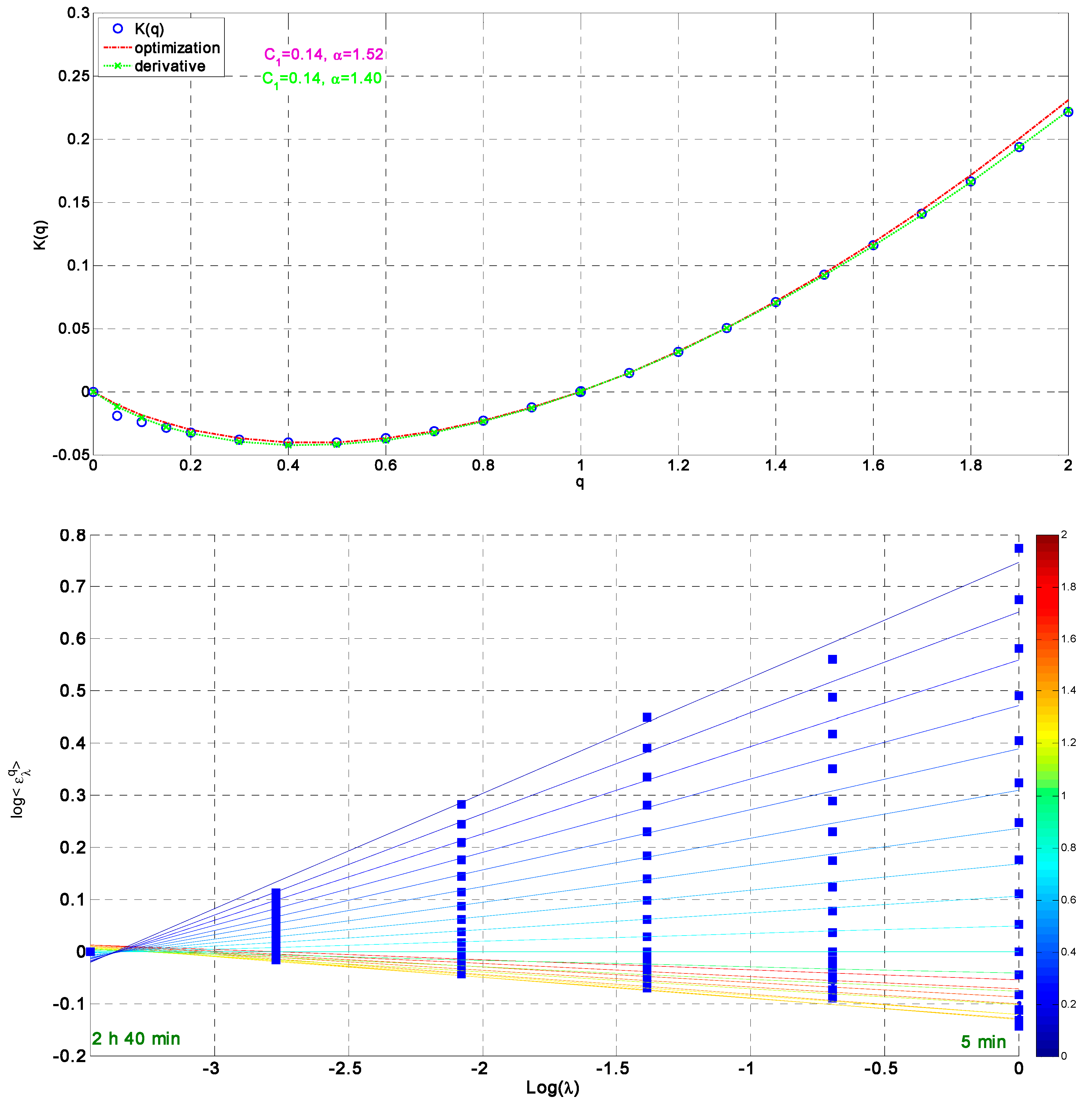
Since the micro-scale regime can be considered as that which governs the rainfall variability within events, five sequences of continuous rain, sufficiently long and relatively intense, were selected.
Figure 4 illustrates the analysis performed for an event lasting 2 h 40 min, at the Mornag station on 23 May 2010. This plot confirms the multifractality of the process at scales between 5 min and 2 h 40 min and therefore the error in estimating α, which yielded a null value in the previous analysis.
The parameters α and C
1, summarized in
Table 4 (7th line),show an increase inα to 1.3 and a decrease in C
1 to 0.15 instead of 0.02 and 0.48, respectively, obtained by analyzing the sequences containing more than 98% of the null values. These results are consistent with those of Pathirana et al. [
22], Verrier et al. [
16], and de Montera et al. [
37] following the use of sequences of continuous rain. From a multitude of events studied, it appears that C
1 and α are correlated with the maximum rainfall amounts: as maximum rainfall increases, both α and
C1 increase. This could explain the behavior of α: when rainfall amounts are sufficiently high to overcome quantization effects, the rainfall field increasingly exhibits multifractal properties.
However, event-by-event analysis is difficult to implement in practice, because of the scarcity of long events, resulting in a limited scale range available for continuous events. In addition, they are insufficiently intense to overcome the discretization problem. Finally, we use very few events, despite the availability of 2.5 years of data, hence the need to propose an alternative (see
Section 4.4).
4.3.2. Meso-Scale and Synoptic Scales Analysis
For the meso-scale regime [2 h 40 min–7 days], uncorrected parameters show slight increases: C
1 from ≈0.48 (micro-scale) to ≈0.58 (meso-scale), and α from ≈0.02 to ≈0.05. However, these values are strongly biased by extreme intermittency (>98% zeros), leading to overestimated C
1 and severely underestimated α. This explains the unusually low α values and discrepancies with literature expectations (
Section 3,
Table 1). After applying empirical bias correction or analyzing continuous rain events, α significantly increases (to ≈0.76–1.4) while C
1 decreases, revealing the expected transition toward more conservative processes at meso-scales.
A slight difference appears between analytical approaches: for differentiated 5 min series (
Table 4, columns 8–9), C
1 ≈ 0.21, whereas for averaged data (2 h 40 min resolution), C
1 ≈ 0.33. At synoptic scales (>7 days), uncorrected parameters are C
1 ≈ 0.21 and α ≈ 0.56. Due to the limited 2.5-year dataset length, these estimates remain tentative and could not be corrected using the proposed empirical method, which requires wider scaling ranges. Nevertheless, preliminary validation with long-term daily records from Tunis-Manoubia (1900–1989) yields consistent values (α ≈ 0.62–0.65, C
1 ≈ 0.27–0.28;
Supplementary Materials), supporting their physical relevance.
Few studies address rainfall characteristics in the semi-arid Mediterranean (
Table 1). Schmitt et al. [
21] analyzed precipitation in Vale Formoso, Portugal, a semi-arid Mediterranean region with climatic conditions similar to our study area. Annual rainfall is comparable (500 mm in Vale Formoso, 444 mm in Tunis) as is potential evapotranspiration (1600 mm vs. 1369 mm). Consequently, similar UM model coefficients are expected. The UM parameters for meso-scale and synoptic regimes are generally consistent: C
1 is about 0.5 for meso-scale and 0.3 for synoptic scales, with a coefficient near 0.6 for synoptic ranges in both studies. Differences include an underestimation of α for meso-scale in Tunis and the absence of a clear 2 h 30 min break in de Lima and Grasman [
21]’s work.
Intermittency leads to errors in estimating multifractal model parameters because rainfall is distributed on a fractal support. When the fractal dimension of this support is less than 1 (instead of 1 for continuous rain), bias arises. Schmitt et al. [
20] accounted for the fractal dimension of the support in calculating the moment scaling function and estimating UM model parameters. Gires [
61] introduced a modified multifractal analysis technique that weights empirical moments by emphasizing non-zero values. Verrier et al. [
16], analyzing intermittency effects on UM parameters using high-resolution data, proposed a semi-empirical formulation based on the difference between tracemoments and simple moments, building on Shmitt et al. [
20]’s approach:
The corrections in Equations (13) and (14) correspond to adding a “beta component” to the UM model as a ‘local’ variant, where
and
are, respectively, the biased fractal codimension and multifractality index and
cf the codimension of the support of rainfall. C
1 and α represent the corrected fractal codimension and multifractality indexes. These formulas explain the overestimation of parameter C
1 and underestimation of the parameter α when analyzing series containing high percentages of zeros. Similarly, the slope of the energy spectrum must be corrected [
16]:
where
is the biased spectral slope and β the true slope.
As noted previously [
16], these equations cannot be applied to obtain the unbiased parameters at micro-scales. In our case, since the
parameter is practically zero, these equations cannot be applied to either micro- or meso-scales. For synoptic scales (>7 days), the fractal codimensions used to adjust the parameters α and
C1 are calculated directly from the fractal dimensions of support calculated by the box-counting method (
cf = 0.9), yielding α greater than 1 (α = 1.2) and C
1 around 0.10. We thus obtained a decrease in the parameter C
1, characterizing the homogeneity of the process, and an increase in α, which measures the degree of multifractality. The interesting aspect here is that if we compare these results with those obtained from the continuous events at the micro-scale (
Table 4, 7th line) we find the parameters at the same order of magnitude.
4.4. Empirical Bias Correction Method
4.4.1. Principles
The approach estimates unbiased micro-scale regime parameters by selecting continuous precipitation sequences, but due to the low resolution of the 5 min data, only a few exceptionally long events are available. To maximize the number and variety of events analyzed, all fixed-length (τ) sequences containing at least one non-zero value were included. Corrections from Equations (13) and (14) were applied conditionally (e.g., cf) to each sequence.
The full two-and-a-half-year dataset was used. Sequences were selected automatically based on the percentage of zero values and shifted in 5 min steps to reduce zeros while preserving a representative sample size, N
0. Biased parameters (
,
) for micro-scale intervals (5 min to 2 h 40 min) were then estimated per sequence, accounting for the zero percentage
as described in Equation (3):
where K is a constant.
As each considered sequence contains at least one non-zero value
, we obtain K = 0. The codimension c
f of the support of each sequence is thus related to the percentage of zeros p
λ with the relationship by:
By substituting into the semi-empirical Equations (13) and (14), the biased parameters can be expressed as functions of the unbiased values and the codimension parameter:
The rainfall series used in this study, characterized by a 5 min resolution and a sequence length of 160 min (25 × 5 min), corresponds to a theoretical normalization constant a = 0.29.
The unbiased parameters are obtained by nonlinear least-squares minimization of the residual sum of squares between observed biased parameters and theoretical predictions from Equation (18), implemented using the fminsearch function (Nelder–Mead simplex algorithm) in MATLAB R2014a. Two optimization strategies are employed: fixing parameter a at its theoretical value while optimizing C1 and α, or allowing all three parameters to vary freely. Initial parameter values are selected based on typical ranges for high-resolution rainfall processes.
Although fminsearch is formally unconstrained, the mathematical structure of Equation (18) implicitly enforces physical constraints ensuring positive parameters consistent with Universal Multifractal theory. Optimization convergence is determined by MATLAB’s default tolerances on both function value and parameter changes. To verify robustness, the optimization is repeated from multiple randomly perturbed initial conditions to confirm convergence to a consistent solution independent of starting values.
No explicit regularization is applied given the substantial overdetermination of the problem, where the number of analyzed sequences greatly exceeds the number of fitted parameters. The validity of fixing parameter a at its theoretical value is assessed by comparing results from constrained and unconstrained optimization approaches.
4.4.2. Application to Micro-Scales Regime
The complete micro-scale analysis workflow is illustrated in
Figure 5 (Panel A). Sequences of 2 h 40 min (λ = 2
5 = 32 time steps at 5 min resolution) were analyzed, as established multifractal methodology requires a minimum scale range spanning 2
4–2
5 points (16–32 samples) for stable estimation of the moment scaling function K(q) across moment orders q = 0 to 2 [
12,
19,
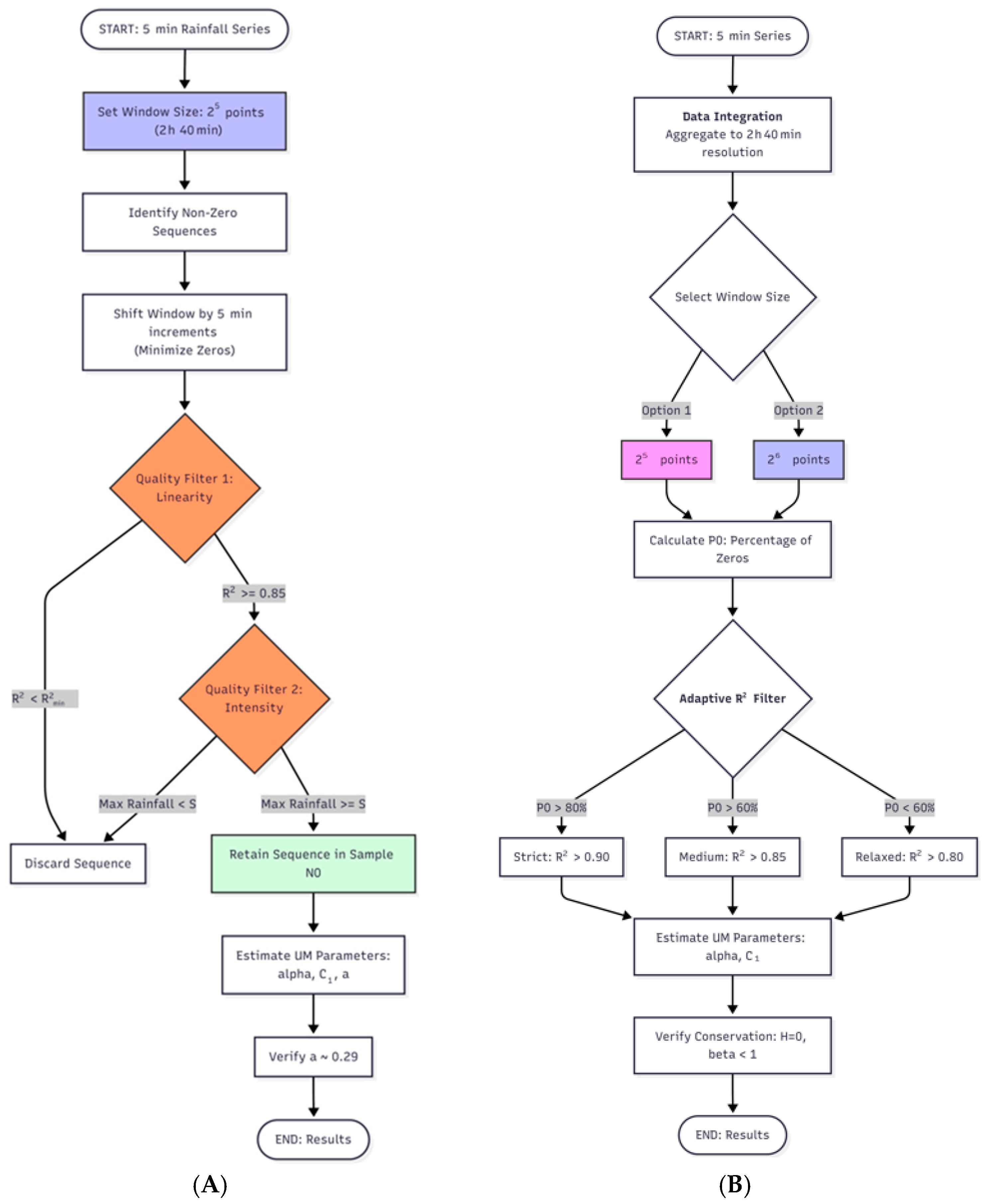
54]. To reduce data quantization effects, parameters are estimated over the 10 min to 2 h 40 min range. Sequences with poor linearity between
and
(R
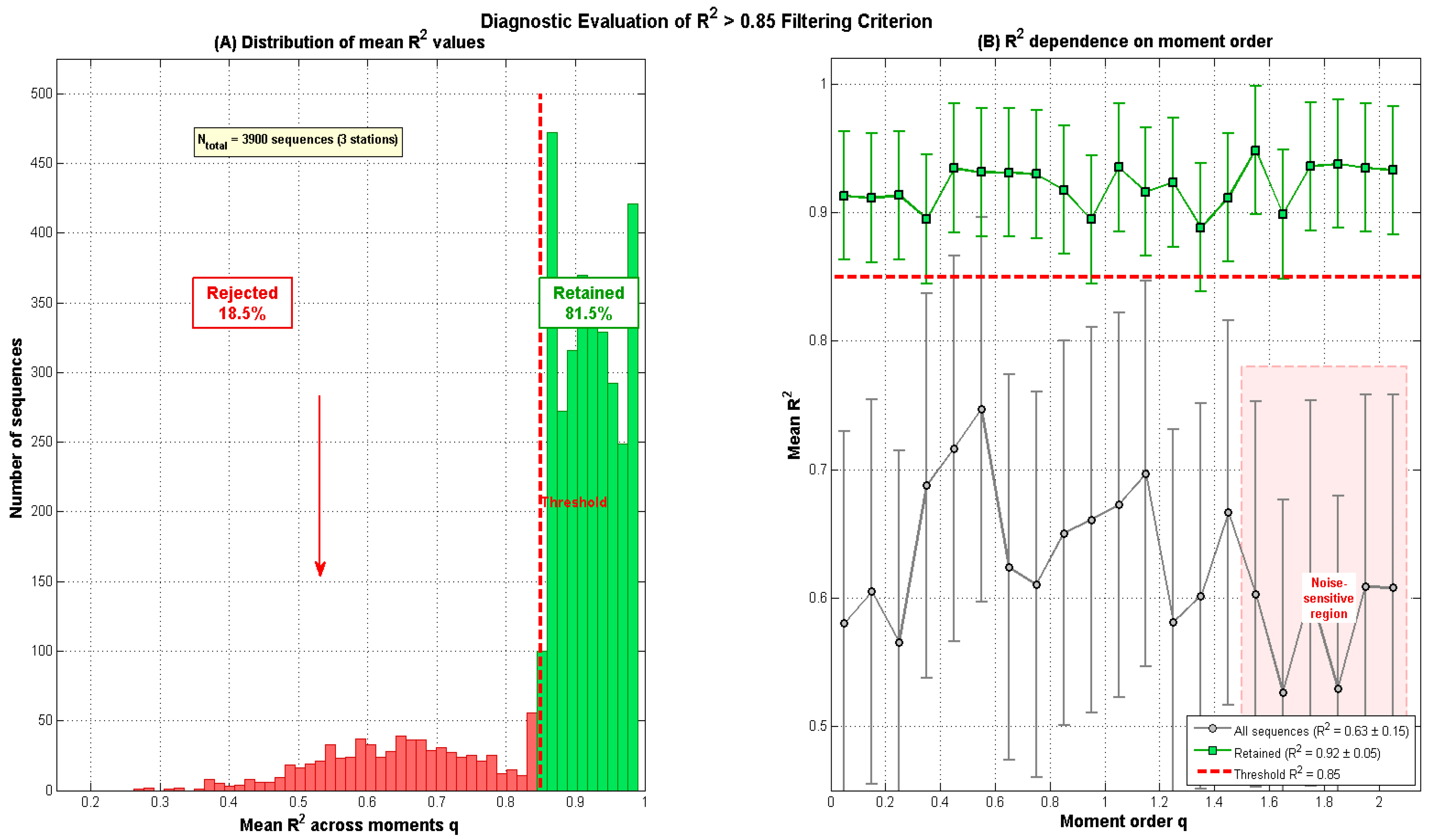
2 ≤ 0.85) are excluded, leaving 1093, 1299, and 787 sequences for the Tunis-Manoubia, Sidi Thabet, and Mornag stations, respectively. The statistical distribution of these values (
Figure 6, Panel A) shows clear bimodal behavior, effectively separating the scaling-compliant sequences from the noise-dominated ones. Sequences with maximum 5 min rainfall intensity below a threshold of 12 mm/h are systematically eliminated. As demonstrated in
Figure 6 (Panel B), this rigorous selection process ensures that the scaling quality remains stable even in the noise-sensitive region (q > 1.5), providing a robust foundation for the estimation of α and C
1. This filtering protocol was optimized to satisfy two critical requirements:
(1) Statistical and Instrumental Robustness: The 12 mm/h threshold corresponds to 10 times the measurement quantum (0.1 mm resolution), providing a necessary margin above the instrumental quantization artifacts that introduce artificial zeros in micro-scale differentiation. Iterative testing (ranging from 6 to 18 mm/h) identified this value as the optimal compromise, maintaining a sample size (N = 248) sufficient for stable parameter estimation (α = 1.63, C1 = 0.07) while ensuring high fit quality (mean R2 > 0.85).
(2) Hydrological Significance and Local Validation: This empirical selection is independently validated by local climatological studies at the Tunis-Manoubia station. Benzarti [
2] demonstrates that events with amounts < 2 mm represent 80–85% of recorded occurrences but are ”insignificant from the rainfall contribution perspective”. Sensitivity analysis confirms that parameter estimates remain stable around this 12 mm/h pivot, whereas lower thresholds lead to unstable α and C
1 values due to the numerical dominance of trace rainfall events.
The codimension
cf obtained by Equation (17) for all the sequences
ranges between 0 and 1 with an average of 0.44.
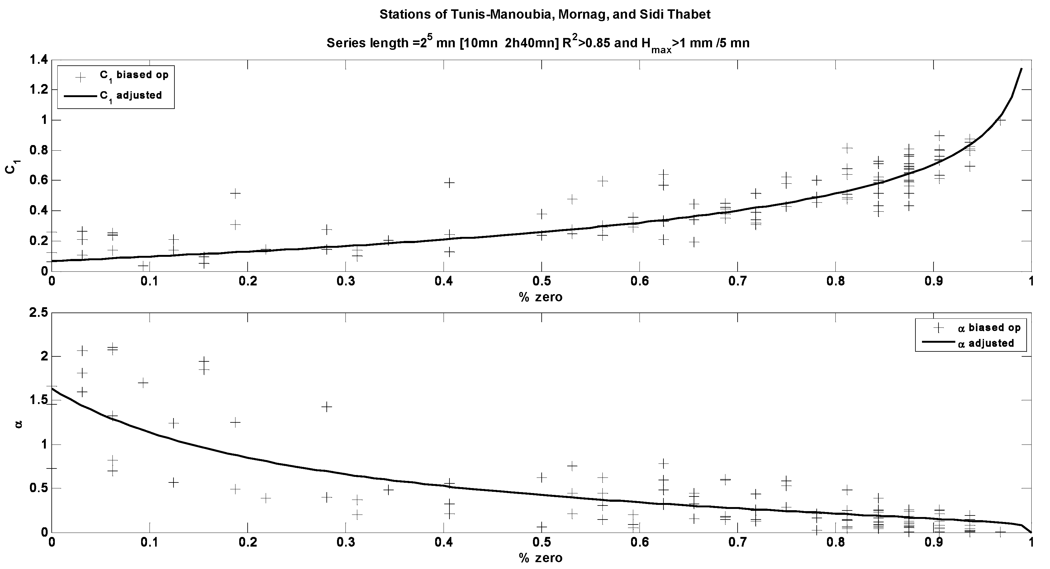
Figure 7 shows the biased parameters
and
as functions of the corresponding
for the 248 selected sequences. The series used here, with
equal to 5 min and a length
τ equal to 2
5 × 5 min, has a theoretical value of the constant a equal to 0.29. In fitting Equation (18) (
Figure 7), we found {α, C
1, a} = {1.6, 0.1, 0.28}. Setting the constant a to its theoretical valuegives similar results (
Table 4, last line). The obtained parameters align well with those derived from the five continuous events discussed in
Section 4.3.1 and closely match the results reported by Verrier et al. [
16], who analyzed data from a similar regime in a temperate region near Paris.
The estimation of β (Equation (10)) using the corrected parameters (α = 1.63, C
1= 0.07) gives a β of 1.13 for the micro-scale regime, a value very close to that estimated from the average spectrum for the wet period outside of summer, which is equal to 1.14 (see
Table 3).
These corrected micro-scale parameters (α = 1.63, C
1 = 0.07;
Table 4, last line, from empirical bias correction applied to 248 sequences) demonstrate strong internal consistency with continuous-event analysis performed on the same dataset (α = 1.40, C
1 = 0.15;
Table 4, line 7, from fiveuninterrupted rain sequences). The corrected α value is 16% higher and C
1 is 53% lower than continuous-event estimates—differences within expected variability given that the correction utilizes 248 sequences spanning varied intensities and intermittency levels (0–100% zeros) versus only fivecontinuous events (0% zeros by definition). Critically, both approaches converge on α > 1, characteristic of unbounded log-Lévy multifractal processes, contrasting sharply with the unrealistic α ≈ 0.02 obtained from the uncorrected analysis of highly intermittent full time series (
Table 4, lines 2–4, >98% zeros). This transformation from monofractal-like (α ≈ 0) to strongly multifractal (α > 1.6) behavior after bias correction validates the effectiveness of our empirical method (
Section 4.4).
The corrected parameters align qualitatively with studies applying different bias correction approaches to intermittent rainfall, despite methodological and contextual differences that preclude direct quantitative comparison. Schmitt et al. [
20] obtained α = 1.55 and C
1 = 0.05 for 10 min Uccle (Belgium) rainfall using a fractal dimension support correction over [10 min–1 day], spanning both our micro-scale convective regime (β > 1) and meso-scale frontal regime (>2 h 30 min, β ≈ 0.5). Verrier et al. [
16] reported α = 1.22 and C
1 = 0.16 using weighted trace moments for Paris DBS data over [32 min–1 week], beginning near our identified regime break. While scale-range differences, distinct correction methodologies (fractal dimension vs. weighted moments vs. our zero-percentage empirical approach), and contrasting climates (temperate oceanic vs. semi-arid Mediterranean with <80% vs. 99% zeros) prevent direct parameter-by-parameter comparison, all three studies consistently demonstrate α > 1 when intermittency bias is addressed—regardless of the correction technique. This convergence across diverse methods and regions provides qualitative validation that our empirical correction successfully removes intermittency artifacts and retrieves physically meaningful rainfall scaling properties for the Tunis semi-arid context. The practical advantage of our approach is its ability to analyze the complete 2.5-year dataset rather than relying on scarce continuous events, improving statistical robustness while achieving comparable parameter recovery.
Table 6 demonstrates that rigorous dual filtering is essential for unbiased multifractal parameter estimation in highly intermittent rainfall data. Quality filtering alone (R
2 ≥0.85) retains sequences affected by quantization artifacts, yielding overestimated α values (1.81), while intensity filtering without quality control includes poorlyscaled sequences. Low intensity thresholds (3.6–6 mm/h) introduce severe systematic bias, underestimating α by up to 17% due to artificial zeros created by the 0.1 mm tipping-bucket resolution, which affects 45% of the observations below 0.3 mm during differentiation. The optimal threshold of 12 mm/h effectively eliminates quantization effects while maintaining adequate statistical power (n = 248 from 3900 initial sequences, representing 6.4% retention of highest-quality events). Spatial consistency analysis across the three independent stations yields α ranging from 1.35 to 1.90 (±17% variability), confirming that observed parameter variations reflect genuine regional heterogeneity rather than methodological artifacts. Cross-validation between constrained optimization (a = 0.29 fixed at theoretical value) and unconstrained optimization (a = 0.28 freely estimated) shows excellent agreement, with only 3.6% difference, thereby validating both the theoretical framework and the empirical correction methodology for handling extreme intermittency in semi-arid Mediterranean rainfall regimes.
4.4.3. Application to Meso-Scale Regime
The meso-scale analysis protocol (
Figure 5, Panel B) operates at coarser temporal resolution. After combining datasets from the Tunis-Manoubia, Sidi Thabet, and Mornag stations to produce 2 h 40 min resolution series, the bias correction method was applied using sequences of 1 week (2
6 points).Unbiased parameters were estimated via the least-squares extrapolation method. The sample selection method (
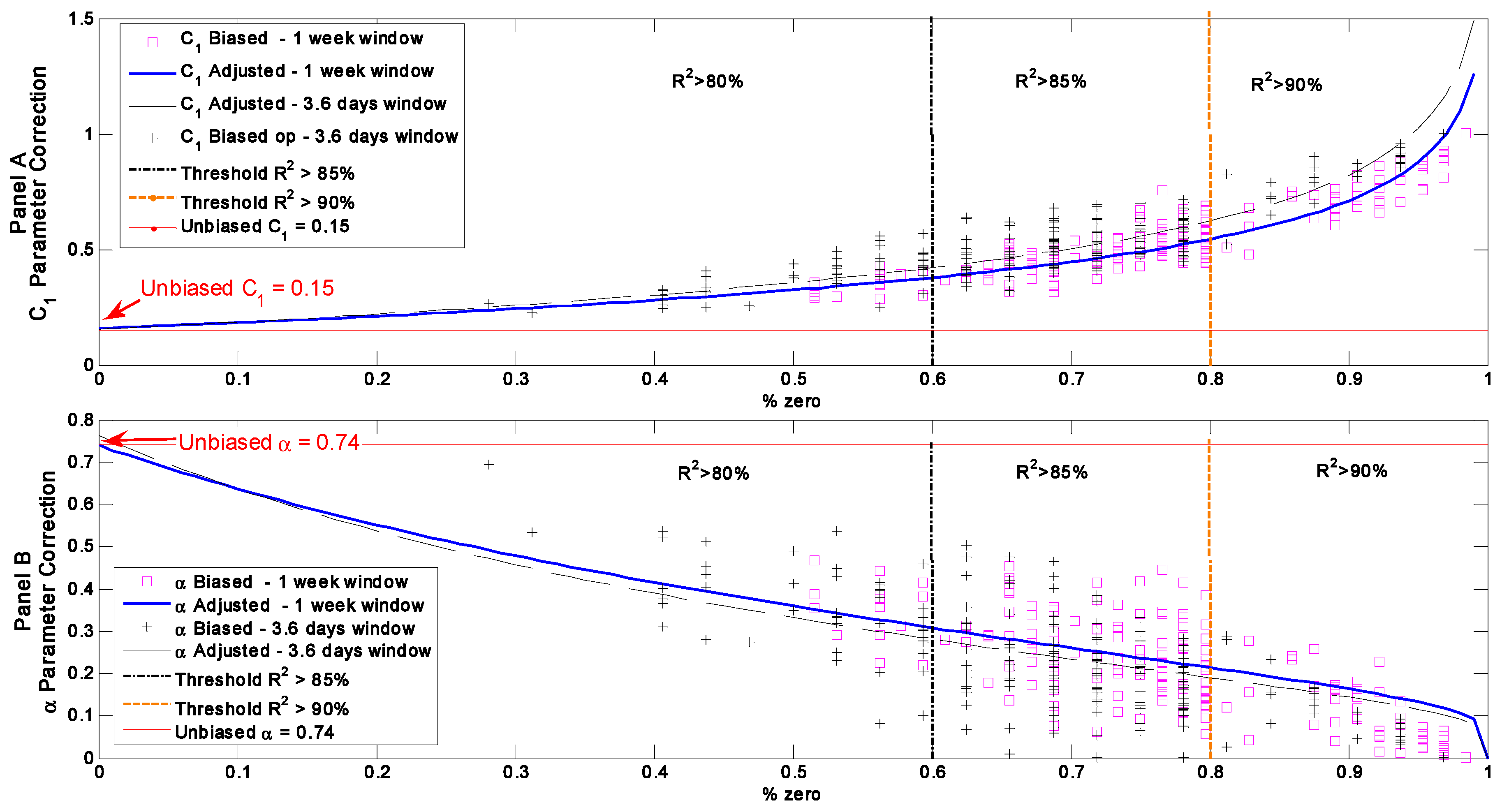
Section 4.4.1) yielded 518 samples. However, as shown in
Figure 8, the high minimum zero-value percentage (approximately 50%) negatively impacts the fit quality. To address the scarcity of samples with low zero percentages, the initial linearity condition (R
2 > 0.85) was adaptively relaxed. Stricter R
2 thresholds were then applied according to the intermittency level: R
2 > 90% for sequences with >80% zeros, >85% for >60%, and >80% for <60% zeros.
The series analyzed have a length of 26 × 2 h 40 min and a theoretical constant a = 0.24. Unbiased parameters α = 0.74 and C1 = 0.15 were estimated. The meso-scale regime yielded a β of 0.79, slightly above the previous maximum of 0.7 but still less than 1. The empirical estimates for the first two regimes reliably capture multifractal parameters and reproduce the non-conservation parameter β.
Figure 8 illustrates the relationship between the percentage of zero values and the biased multifractal estimates (
1 and
1). All individual data points (squares and crosses) represent biased estimates. The unbiased parameters are determined by the y-axis intercept, where the intermittency effect is null (0% zeros).
The results for the 1-week window (α = 0.74, C1 = 0.16) and the 3.6-day window (α = 0.76, C1 = 0.15) show remarkable consistency. Consequently, imposing additional constraints on the H parameter did not significantly improve estimation quality but restricted the sample distribution. Therefore, the robust extrapolation toward the 0% zero-value intercept remains the most reliable method for identifying the true universal multifractal parameters.
4.4.4. Method Advantages and Limitations
The proposed empirical bias correction method offers several key advantages over traditional multifractal analysis approaches when applied to highly intermittent rainfall data. First, it enables utilization of the complete dataset rather than restricting analysis to rare continuous events, increasing usable sample size by two orders of magnitude (from 5 to 248 sequences in this study, representing 0.1% to 6.4% of available data). This substantial sample expansion provides sufficient statistical power for robust parameter estimation and spatial validation across multiple stations. Second, the method explicitly quantifies for the physical relationship between zero-value percentage and parameter bias through Equation (18), offering a theoretically-grounded correction rather than ad hoc adjustments. Third, dual filtering criteria (R2 ≥ 0.85, Hmax > 12 mm/h) systematically separate genuine multifractal scaling from measurement artifacts, addressing both scaling quality and quantization bias. Fourth, the approach demonstrates practical applicability even for sequences with 50% zeros, extending multifractal analysis to moderately intermittent regimes where traditional methods remain applicable but biased. Finally, validation through multiple independent lines of evidence—convergence of fitted parameter a toward theoretical value (0.28 vs. 0.29), consistency with continuous-event estimates (α = 1.63 vs. 1.40), and inter-station robustness (α = 1.35–1.90)—provides confidence in recovered parameters.
However, several limitations constrain the method’s applicability. First, it requires a diverse sample size of sequences spanning a wide range of zero percentages (ideally 0–100%) for stable parameter estimation via least-squares optimization; consequently, application to very short datasets (<1 year) may yield unreliable results due to insufficient variability in intermittency levels. Second, the Hmax threshold necessary to eliminate quantization artifacts introduces a selection bias by excluding light precipitation events, potentially underrepresenting stratiform rainfall characteristics and limiting applicability to meso-scale parameter estimation. Third, the method addresses temporal intermittency but does not account for spatial intermittency, which may introduce additional bias in spatially-distributed multifractal analysis. Fourth, parameter correction relies on the assumption that Equation (18) adequately captures the bias structure across all scales; preliminary results suggest this assumption holds for micro- and meso-scales but remains unvalidated for synoptic scales due to dataset length limitations. Fifth, the correction is specific to the Universal Multifractal framework and may not directly transfer to alternative multifractal formalisms (e.g., canonical cascades, wavelet-based methods). Finally, while the method successfully recovers unbiased α and C1 parameters, it does not address potential biases in higher-order multifractal statistics (e.g., extreme value distributions, probability density functions), which warrant future investigation. Despite these limitations, the method represents a practical advance for multifractal characterization in semi-arid and other highly intermittent rainfall regimes where data scarcity has historically precluded reliable parameter estimation.