Consensus Control of Robot Fractional-Order MAS Based on FOILC with Time Delay

Abstract

In this paper, we investigate the finite-time consensus problem of a fractional-order multi-agent system with repetitive motion. The system under consideration consists of robotic agents with a leader and a fixed communication topology. A distributed open-closed-loop PDα fractional-order iterative learning control (FOILC) algorithm is proposed. The finite-time uniform convergence of the proposed algorithm is analyzed, and sufficient convergence conditions are derived. The theoretical analysis demonstrates that, as the number of iterations increases, each agent can achieve complete tracking within a finite time by appropriately selecting the gain matrices. Simulation results are presented to verify the effectiveness of the proposed method.

1. Introduction

The multi-agent systems (MASs) composed of multiple robots can accomplish large-scale and complex tasks through communication, coordination, and cooperation. Their operational efficiency and overall performance are significantly superior to those of a single-agent system. Consequently, MASs have been widely applied in various fields, such as mobile robot transportation, 3D printing, welding, and other industrial applications [1,2]. The consensus problem, which is a representative topic in the cooperative control of MASs, refers to the design of appropriate control algorithms that enable the states or outputs of all agents to converge to a common value within a finite time. Therefore, coordination and consensus problems in multi-agent systems have attracted extensive attention from researchers, resulting in a high volume of significant research [3,4,5,6].

However, most of the existing literature on multi-agent consensus is based on integer-order system descriptions, in which the dynamics of robots are modeled using integer-order differential equations [7,8]. In complex natural environments, such as material mechanics, motor systems, robotic systems, and, in particular, robot dynamics, fractional calculus provides a more accurate description than traditional integer-order calculus [9,10]. Regarding the research on fractional-order systems, Tusset et al. develops a fractional-order bioreactor temperature model that accounts for asymmetric heat transfer via Riemann–Liouville operators, and designs a reduced-order LQR controller acting on jacket flow, which is shown to robustly and efficiently maintain reactor temperature while remaining practical for real applications [11]. The work in [12] addresses the lack of a unified theoretical framework for the robustness of fractional-order systems against parameter perturbations and time-delay variations. A robustness analysis framework was constructed, providing both theoretical foundations and computational tools for robustness analysis of fractional-order systems. In [13], fractional-order control strategies for multi-agent systems with time delays were studied. Fractional-order P controllers were designed based on the generalized Nyquist criterion, and a traversal method was proposed to determine feasible controller parameter ranges for multi-robot and distributed cooperative systems. Bappa et al. investigated controller design and stability analysis for fractional-order nonlinear time-delay systems, proposing two delay-independent stability criteria. Nonlinear terms were compensated through feedback controllers, and the system stability was verified using Lyapunov functions [14]. The above studies primarily focused on the “mathematical analysis” and “model formulation” of fractional-order systems. Strictly speaking, integer-order systems can be regarded as special cases of fractional-order systems. Therefore, with the increasing interest in multi-agent systems, many researchers have gradually shifted their focus from integer-order models to fractional-order models [11,12,13,14].

In the field of fractional-order control systems, Yu et al. were among the first to investigate the consensus control problem of fractional-order multi-agent systems (FOMASs), and established fundamental convergence criteria for leader–follower fractional-order multi-agent systems [11,12]. Subsequently, Bai et al. [13] studied the consensus problem of fractional-order multi-agent systems under both fixed reference states and time-varying reference states. Similarly, the work in [14] introduced and analyzed the concept of consensus in fractional-order dynamics, and proposed a consensus control algorithm based on relative output measurements. Furthermore, Yu et al. employed graph theory and Lyapunov-based methods to investigate the consensus problem of nonlinear FOMASs with a leader, and derived consensus criteria for nonlinear fractional-order multi-agent systems. On this basis, further studies on nonlinear FOMASs were conducted, and stability theories for fractional differential systems were developed using matrix inequalities and Lyapunov stability analysis [15,16]. In addition, the work in [17] presented necessary and sufficient conditions for the consensus control of FOMASs with leaders, and designed an observer-based approach to solve the consensus problem. Moreover, adaptive control and sliding mode control methods were proposed in [18,19], respectively, to address the consensus control problem of fractional-order multi-agent systems.

However, most of the aforementioned studies focused on asymptotic consensus convergence, whereas fractional-order multi-agent systems with repetitive operation characteristics, such as coordinated multi-manipulator operations on production lines, typically require complete consensus within a finite time interval. Obviously, the existing results are insufficient to meet such practical requirements. Among the existing control strategies, iterative learning control (ILC) is capable of achieving complete tracking within a finite time interval for systems performing repetitive tasks. For integer-order multi-agent systems (IOMASs), a substantial number of studies have applied ILC to various system models and achieved satisfactory results [20,21,22]. In contrast, research on fractional-order iterative learning control (FOILC) for fractional-order multi-agent systems remains very limited. Moreover, in practical engineering systems, owing to the characteristics of digital signal processors (DSPs), communication networks, and other processing units, state delays are often inevitable. Therefore, investigating the consensus problem of FOMASs with state delays is of significant practical and engineering relevance.

In this paper, considering the existence of time delays, three PDα-type fractional-order iterative learning control (FOILC) schemes, namely, open-closed-loop FOILC, closed-loop FOILC, and open-loop FOILC, are proposed to address the consensus problem of robot-based fractional-order multi-agent systems (FOMASs). The proposed PDα-type FOILC law integrates an open-loop component, which utilizes the control input from the previous iteration, and a closed-loop component, which exploits the real-time tracking error in the current iteration. This combined structure effectively incorporates historical learning information while responding to current disturbances, thereby accelerating convergence and enhancing system robustness. Based on graph theory, norm theory, and fundamental results from fractional calculus, the finite-time consensus convergence of the proposed algorithms for FOMASs with time delays have been rigorously analyzed and theoretically established. Finally, numerical simulations were conducted to verify the effectiveness of the proposed control strategies, and comparative analyses were performed to illustrate their respective performance characteristics.

2. Basic Knowledge and Problem Description

2.1. Graph Theory

We consider a system consisting of n fractional multi-agents. The communication connections between different individuals constitute a network topology $\mathit{G}$. And $\mathit{G}=\{\mathit{V},\mathit{E},\mathit{M}\}$ represents the directed network weighted graph, where $\mathit{V}=\{v_1,\cdots ,v_n\}$ is the set of nodes and $\mathit{E}\in \mathit{V}\times \mathit{V}$ is the set of edges in the network topology, $I=\{1,2,\cdots ,n\}$ representing the index set of the node. The adjacency matrix of the network topology is represented by $\mathit{M}={(a_{ik})}_{n\times n}$, where $a_{ik}$ represents the connection weight from node i to node k. If node i transmits information to node k, then $a_{ik}>0$, otherwise $a_{ik}=0$. We also assume that each node in the network has no self-connection phenomenon, that is $a_{ii}=0$ for $i\in \mathit{I}$.

We define the set of neighbor nodes of network node i as ${\mathit{N}}_i=\{k:a_{ik}>0\}$. We define $\mathit{D}=diag\{d_i,i=1,\cdots ,N\}$, where $d_i={\displaystyle {\sum }_{k=1}^N{a}_{ik}}$ is the sum of the elements in the i-th row of the network adjacency matrix M. As such, the Laplacian matrix of graph G is $\mathit{L}=\mathit{D}-\mathit{M}$. For the two nodes i and k, if there is a set of subscripts $\{k_1,\cdots ,k_l\}$ that satisfy $a_{i{k}_1}>0$, $a_{i{k}_2}>0$, $\cdots$, and $a_{i{k}_l}>0$, then there is an information transmission channel between node i and node k, and it also means that node k can receive the information of node i. If a path can be found to reach any node in the graph for node i, it means that node i becomes globally reachable.

Lemma 1. 

Assumes a fractional-order multi-agent system comprising n autonomous individuals, where its connection topology is a directed weighted network and there is at least one globally reachable node in the network. Consequently, the rank of the Laplacian matrix L of the connection topology graph is  $N-1$, and there is a 0 eigenvalue. The corresponding feature vector is  ${\xi }_0=c{[1,\cdots ,1]}^T.$

2.2. Fractional Calculus and Norm Theories

The fractional calculus used in this paper is defined as follows [23]:

Definition 1. 

In the interval  $[t_0,t]$, the left-sided and the right-sided Riemann-Liouville’s fractional integral of order  $\alpha >0$  for a function  $\mathit{f}$  are defined as

$${}_{t_0}D_t^{-\alpha }f(t)={\displaystyle \frac{1}{\Gamma (\alpha )}}{\displaystyle {\int }_{t_0}^t{(t-\tau )}^{\alpha -1}f(\tau )}d\tau ,(t>t_0)$$

(1)

$${}_{t}D_T^{-\alpha }\mathit{f}(t)={\displaystyle \frac{1}{\Gamma (\alpha )}}{\displaystyle {\int }_t^T{(\tau -t)}^{\alpha -1}f(\tau )}d\tau ,(t<T)$$

(2)

where  $\Gamma (\cdot )$  is Gamma function.

The left-sided and the right-sided Caputo derivative are given by

$${}_{t_0}{}^{C}D_t^{\alpha }f(t)={}_{t_0}D_t^{-\left(\right[\alpha ]-\alpha +1)}\left[{\displaystyle \frac{d^{[\alpha ]+1}}{d{t}^{[\alpha ]+1}}}f(t)\right],(t>t_0),$$

(3)

$${}_t{}^{C}D_T^{\alpha }f(t)={}_{t}D_T^{-\left(\right[\alpha ]-\alpha +1)}\left[{\displaystyle \frac{d^{[\alpha ]+1}}{d{t}^{[\alpha ]+1}}}f(t)\right],(t<T)$$

(4)

where $\alpha \in {\mathbf{R}}^{+}$, $[\alpha ]$ is the integral part of $\alpha$.

Lemma 2. 

For the continuous function  $\mathit{f}(\mathit{x}(t),t)$, as shown in (4),

$$\left\{\begin{array}{c}{}_{t_0}{}^{C}D_t^{\alpha }\mathit{x}(t)=\mathit{f}(\mathit{x}(t),t)\\ \mathit{x}(t_0)=\mathit{x}(0)\hfill \end{array},0<\alpha <1\right.$$

(5)

Then, the equivalent Volterra type nonlinear integral equation for the initial value problem is

$$\mathit{x}(t)=\mathit{x}(0)+{\displaystyle \frac{1}{\mathit{\Gamma }(\alpha )}}{\displaystyle {\int }_{t_0}^t{(t-\tau )}^{\alpha -1}\mathit{f}(\mathit{x}(\tau ),\tau )}\mathrm{d}\tau$$

(6)

We use $ℝ$ and $ℂ$ to denote any set of real numbers and complex numbers, and use $\mathbb{N}$ to denote the set of natural numbers. For a vector $\mathit{x}={[x_1,x_2,\cdots ,x_n]}^{\mathrm{T}}\in {ℝ}^n$, $\left|\mathit{x}\right|$ represents the $l_p$ norm of the vector $\mathit{x}$, where $1\le p\le \infty$. In fact, when p takes 1, 2 and ∞, we have $|\mathit{x}{|}_1={\displaystyle {\sum }_{k=1}^n\left|x_k\right|}$, ${\left|\mathit{x}\right|}_2=\sqrt{{\mathit{x}}^T\mathit{x}}$, and $|\mathit{x}{|}_{\infty }=\underset{k=1,\cdots ,n}{\max }|x_k|$. For the matrix $\mathit{A}\in {ℝ}^{n\times n}$, $‖\mathit{A}‖$ represents the matrix norm and $\rho (\mathit{A})$ is the spectral radius of the matrix $\mathit{A}$ . In this paper, $\otimes$ means the Kronecker product, ${\mathit{I}}_m$ represents the $m\times m$ identity matrix.

2.3. Fractional Multi-Agent Model with State Delay

We assume that the fractional multi-agent with leader includes N multi-agents, defined as 1, 2, 3,…, N. The model of each fractional multi-agent is described as:

$$\left\{\begin{array}{l}{D}^{\alpha }{\mathit{x}}_{i,j}(t)=\mathit{A}{\mathit{x}}_{i,j}(t-\tau )+\mathit{B}{\mathit{u}}_{i,j}(t)\\ {\mathit{y}}_{i,j}(t)=\mathit{C}{\mathit{x}}_{i,j}(t)\end{array}\right.$$

(7)

where ${\mathit{x}}_{i,j}(t)\in {ℝ}^m$, ${\mathit{u}}_{i,j}(t)\in {ℝ}^{m1}$, and ${\mathit{y}}_{i,j}(t)\in {ℝ}^{m2}$ are the state, input, and output vectors of the j-th agent at the i-th iteration, respectively, $D^{\alpha }{\mathit{x}}_{i,j}(t)$ means the $\alpha$-order derivative of ${\mathit{x}}_{i,j}(t)$, i is the number of iterations, and j means the j-th agent. The matrices $\mathit{A}\in {ℝ}^{m\times m}$, $\mathit{B}\in {ℝ}^{m\times m1}$, and $\mathit{C}\in {ℝ}^{m2\times m}$ are constant, while $t\in [0,T]$ and the initial condition function ${\mathit{x}}_{i,j}(t)=\mathit{\psi }(t)$ for $t\in [0,\tau ]$ and $\alpha \in (0,1)$.

Formula (7) can be written in the multi-agent vector form as

$$\left\{\begin{array}{l}{D}^{\alpha }{\mathit{x}}_i\left(t\right)=\left(I_N\otimes A\right){\mathit{x}}_i\left(t-\tau \right)+\left(I_N\otimes B\right){\mathit{u}}_i\left(t\right)\\ {\mathit{y}}_i\left(t\right)=\left(I_N\otimes C\right){\mathit{x}}_i\left(t\right)\end{array}\right.$$

(8)

where ${\mathit{x}}_i(t)={[{\mathit{x}}_{i,1}{(t)}^T,{\mathit{x}}_{i,2}{(t)}^T,\cdots ,{\mathit{x}}_{i,N}{(t)}^T]}^T$, ${\mathit{u}}_i\left(t\right)={\left[{\mathit{u}}_{i,1}^T\left(t\right),{\mathit{u}}_{i,2}^T\left(t\right),\cdots ,{\mathit{u}}_{i,N}^T\left(t\right)\right]}^T$, ${\mathit{y}}_i\left(t\right)={\left[{\mathit{y}}_{i,1}^T\left(t\right),{\mathit{y}}_{i,2}^T\left(t\right),\cdots ,{\mathit{y}}_{i,N}^T\left(t\right)\right]}^T$, and ${\xi }_i(t)={[{\xi }_{i,1}{(t)}^T,{\xi }_{i,2}{(t)}^T,\cdots ,{\xi }_{i,N}{(t)}^T]}^T$, with $\otimes$ representing the Kronecker product. In this paper, the expected trajectory ${\mathit{y}}_d(t)$ is generated by the leader as expressed in Formula (6) in the time interval $[0,T]$, and the leader is defined as

$$\left\{\begin{array}{l}{D}^{\alpha }{\mathit{x}}_d(t)=\mathit{A}{\mathit{x}}_d(t-\tau )+\mathit{B}{\mathit{u}}_d(t)\\ {\mathit{y}}_d(t)=\mathit{C}{\mathit{x}}_d(t)\end{array}\right.$$

(9)

where ${\mathit{u}}_d(t)$ is the desired input.

Due to the limitations with either communication or sensors, the leader can only communicate with some multi-agents. The communication network can be defined as $\mathit{G}\{\mathit{V},\mathit{E}\}$ and the leader’s number as 0, and the complete graph containing the leader can be expressed as $\overline{\mathit{G}}=\{0\cup \mathit{V},\overline{\mathit{E}}\}$, where $\overline{\mathit{E}}$ represents the corresponding edge in the new graph. The main task of this paper is to design a suitable fractional-order iterative learning controller to ensure that each multi-agent converges to the desired trajectory in the sense of the new graph $\overline{\mathit{G}}$.

Our definition for ${\xi }_{i,j}(t)$ as distributed error is as follows:

$${\xi }_{i,j}(t)={\displaystyle {\sum }_{k\in N_j}{a}_{j,k}({\mathit{y}}_{i,k}(t)-{\mathit{y}}_{i,j}(t))}+d_k({\mathit{y}}_d(t)-{\mathit{y}}_{i,j}(t))$$

(10)

where $a_{j,k}$ is the weight of the $(j,k)$-th neighborhood of the adjacent-order matrix $\mathit{M}$, ${\mathit{N}}_j$ is the domain set of the j-th multi-agent, and $d_k$ is the sum of the elements in the i-th row of the network adjacency matrix. If $d_j=1$, then the j-th multi-agent can receive information from the leader, that is $(0,j)\in \overline{\mathit{E}}$, otherwise $d_j=0$. The error is defined as ${\mathit{e}}_{i,j}(t)={\mathit{y}}_d(t)-{\mathit{y}}_{i,j}(t)$.

Then, the open-closed $P{D}^{\alpha }$ type FOILC is designed as:

$${\mathit{u}}_{i+1,j}(t)={\mathit{u}}_{i,j}(t)+{\mathit{\Gamma }}_{P1}{\xi }_{i,j}(t)+{\mathit{\Gamma }}_{D1}{{\xi }_{i,j}}^{\left(\alpha \right)}(t)+{\mathit{\Gamma }}_{P2}{\xi }_{i+1,j}(t)+{\mathit{\Gamma }}_{D2}{{\xi }_{i+1,j}}^{\left(\alpha \right)}(t)$$

(11)

where $\alpha$ denotes the α-th order derivative of ${\xi }_{i,j}(t)$, and according to Equation (10) and the error expression we have:

$${\xi }_{i,j}(t)={\displaystyle {\sum }_{k\in {\mathit{N}}_j}{a}_{j,k}({\mathit{e}}_{i,j}(t)-{\mathit{e}}_{i,k}(t))}+d_k{\mathit{e}}_{i,j}(t)$$

(12)

The column vector is defined as ${\mathit{x}}_i(t)={[{\mathit{x}}_{i,1}{(t)}^T,{\mathit{x}}_{i,2}{(t)}^T,\cdots ,{\mathit{x}}_{i,N}{(t)}^T]}^T$, ${\mathit{e}}_i(t)={[{\mathit{e}}_{i,1}{(t)}^T,{\mathit{e}}_{i,2}{(t)}^T,\cdots ,{\mathit{e}}_{i,N}{(t)}^T]}^T$, and ${\xi }_i(t)={[{\xi }_{i,1}{(t)}^T,{\xi }_{i,2}{(t)}^T,\cdots ,{\xi }_{i,N}{(t)}^T]}^T$. Therefore, Equation (12) can be rewritten as

$${\xi }_i(t)=((\mathit{L}+\mathit{D})\otimes {\mathit{I}}_m){\mathit{e}}_i(t)$$

(13)

where L is the Laplacian matrix of graph $\overline{\mathit{G}}$ and $\mathit{D}=diag\{d_i,i=1,\cdots ,N\}$, and m is the dimension of state ${\mathit{x}}_{i,j}(t)$.

According to (13), the controller in Equation (10) is written as a matrix vector as follows:

$$\begin{array}{l}{\mathit{u}}_{i+1}(t)={\mathit{u}}_i(t)+((\mathit{L}+\mathit{D})\otimes {\mathit{\Gamma }}_{P1}){\mathit{e}}_i(t)+((\mathit{L}+\mathit{D})\otimes {\mathit{\Gamma }}_{D1}){{\mathit{e}}_i}^{\left(\alpha \right)}(t)+\\ ((\mathit{L}+\mathit{D})\otimes {\mathit{\Gamma }}_{P2}){\mathit{e}}_{i+1}(t)+((\mathit{L}+\mathit{D})\otimes {\mathit{\Gamma }}_{D2}){{\mathit{e}}_{i+1}}^{\left(\alpha \right)}(t)\end{array}$$

(14)

In order to facilitate analysis, we define ${\lambda }_j$ and $j=1,2,\cdots ,N$ as the eigenvalues of the matrix $\mathit{L}+\mathit{D}$.

Remark 1. 

The proposed PDα-type FOILC law combines an open-loop component (utilizing the control input from the previous iteration) and a closed-loop component (utilizing the real-time tracking error from the current iteration). This structure leverages past experience while reacting to current disturbances, aiming to accelerate convergence and improve robustness.

3. Convergence Analysis

In order to facilitate the convergence analysis of the proposed algorithm, the following assumptions were established:

Assumption 1. 

The initial state of each subsystem (6) when it repeatedly runs on the interval  $[0,T]$ is equal to the expected initial state, that is, for all  $k$, ${\mathit{x}}_{i,k}(0)={\mathit{x}}_d(0)$  is held.

Remark 2. 

In order to ensure more perfect tracking results, the initial value conditions in Assumption 2 need to be established in the ILC design. However, if the assumption does not hold, Optimal tracking can never be realized without an optimal initial condition. The initial state learning control is discussed in [24].

Assumption 2. 

The augmented communication graph $\overline{\mathit{G}}$ contains a directed spanning tree with the leader (node 0) as the root.

Remark 3. 

This Assumption 2 is a pre-requisite for the FOMASs consensus tracking problem which states that all followers have access to the leader. Otherwise, due to the absence of data to make their control inputs accurate, the isolated agents cannot track the leader’s trajectory.

Theorem 1. 

Consider the fractional-order multi-agent system (8) under the conditions of graph  $\overline{\mathit{G}}$, assumptions 1–2. If the communication graph satisfies Assumption 2, and the distributed open-closed-loop PD^α-type ILC law (13) is applied with learning gain matrices  ${\mathit{\Gamma }}_{P1}$,  ${\mathit{\Gamma }}_{P2}$,  ${\mathit{\Gamma }}_{D1}$,  ${\mathit{\Gamma }}_{D2}$  satisfying the following conditions:

(1) 

$\mathit{\Gamma }(\alpha )-\left|\right|{(t)}^{\alpha -1}({\mathit{I}}_n\otimes \mathit{A})|{|}_1>0$

(2) 

$0<{\rho }_1<1,0<{\rho }_2<1,{\displaystyle \frac{{\rho }_1}{{\rho }_2}}<1$,

where

$${\rho }_1=|\mathit{I}-((\mathit{L}+\mathit{D})\otimes {\mathit{\Gamma }}_{D1})({\mathit{I}}_n\otimes \mathit{C})({\mathit{I}}_n\otimes \mathit{B})||+{\beta }_1,$$

$${\rho }_2=\left|\right|\mathit{I}+((\mathit{L}+\mathit{D})\otimes {\mathit{\Gamma }}_{D2})({\mathit{I}}_n\otimes \mathit{C})({\mathit{I}}_n\otimes \mathit{B})\left|\right|-{\beta }_2,$$

$${\beta }_g={\displaystyle \frac{\left|\right|((\mathit{L}+\mathit{D})\otimes {\mathit{\Gamma }}_{Pi})({\mathit{I}}_n\otimes \mathit{C})\left|\right|+\left|\right|((\mathit{L}+\mathit{D})\otimes {\mathit{\Gamma }}_{Di})({\mathit{I}}_n\otimes \mathit{C})({\mathit{I}}_n\otimes \mathit{A}))||}{\mathit{\Gamma }(\alpha )-\left|\right|{(t)}^{\alpha -1}({\mathit{I}}_n\otimes \mathit{A})|{|}_1}}||{(t)}^{\alpha -1}({\mathit{I}}_n\otimes \mathit{B})|{|}_1,g=1,2$$

then, as the iteration number increases i→∞, the tracking error  ${\mathit{e}}_{i,j}(t)$  converges uniformly to zero on [0, T], i.e.,  $\underset{i\to \infty }{\lim }{y}_{i,j}\left(t\right)=y_d\left(t\right)$,  $\underset{i\to \infty }{\lim }{u}_{i,j}\left(t\right)=u_d\left(t\right)$  for all j.

Where $\mathit{I}$ is the unit matrix, and $\rho$ is a constant, $\mathit{H}=\mathit{L}+\mathit{D}$, $\mathit{L}$ is the Laplacian matrix, $\mathit{D}=diag\{d_i,i=1,\cdots ,N\}$.

Proof. 

We define

$$\left\{\begin{array}{l}\delta {\mathit{x}}_{i,j}(t)={\mathit{x}}_d(t)-{\mathit{x}}_{i,j}(t)\\ \delta {\mathit{u}}_{i,j}(t)={\mathit{u}}_d(t)-{\mathit{u}}_{i,j}(t)\end{array}\right.$$

(15)

where $\delta {\mathit{x}}_i(t)$ and $\delta {\mathit{u}}_i(t)$ are the vector forms of $\delta {\mathit{x}}_{i,j}(t)$ and $\delta {\mathit{u}}_{i,j}(t)$, and when $t\in [-h,0](h>0)$, we have

$$\delta {\mathit{x}}_i(t)=0$$

(16)

Hence

$$\begin{array}{l}||\delta {\mathit{x}}_i(t-\tau )|{|}_p={[{\displaystyle {\int }_0^t{(\underset{1\le j\le n}{\max }|\delta x_{i,j}(s-\tau )|)}^p\mathrm{d}s}]}^{1/p}\\ \hfill \hspace{1em}\hspace{1em} ={[{\displaystyle {\int }_{-\tau }^{t-\tau }{(\underset{1\le j\le n}{\max }|\delta x_{i,j}(s)|)}^p\mathrm{d}s}]}^{1/p}\hfill \\ \hfill \hspace{1em}\hspace{1em} ={[{\displaystyle {\int }_0^{t-\tau }{(\underset{1\le j\le n}{\max }|\delta x_{i,j}(s)|)}^p\mathrm{d}s}]}^{1/p}\hfill \\ \hfill \hspace{1em}\hspace{1em} \le {[{\displaystyle {\int }_0^t{(\underset{1\le j\le n}{\max }|\delta x_{i,j}(s)|)}^p\mathrm{d}s}]}^{1/p}\hfill \\ \hspace{1em}\hspace{1em} \hspace{1em} =||\delta {\mathit{x}}_i(t)|{|}_p\end{array}$$

(17)

According to the definition of error and Assumption 1, we have

$$\begin{array}{l}{\mathit{e}}_i^{(\alpha )}(t)={\mathit{y}}_d^{(\alpha )}(t)-{\mathit{y}}_i^{(\alpha )}(t)\\ \hspace{1em} =({\mathit{I}}_n\otimes \mathit{C})({\mathit{x}}_d^{(\alpha )}(t)-{\mathit{x}}_i^{(\alpha )}(t))\hfill \\ \hspace{1em} =({\mathit{I}}_n\otimes \mathit{C})\delta {\mathit{x}}_i^{(\alpha )}(t)\\ \hspace{1em} =({\mathit{I}}_n\otimes \mathit{C})({\mathit{I}}_n\otimes \mathit{A})\delta {\mathit{x}}_i(t-\tau )+({\mathit{I}}_n\otimes \mathit{C})({\mathit{I}}_n\otimes \mathit{B})\delta {\mathit{u}}_i(t)\end{array}$$

(18)

Based on Lemma 2 we have

$$\begin{array}{c}{\mathit{x}}_i(t)={\mathit{x}}_i(0)+{\displaystyle \frac{1}{\mathit{\Gamma }(\alpha )}}{\displaystyle {\int }_0^t{(t-s)}^{\alpha -1}(({\mathit{I}}_n\otimes \mathit{A}){\mathit{x}}_i(s-\tau )+({\mathit{I}}_n\otimes \mathit{B}){\mathit{u}}_i(s))\mathrm{d}s}\\ ={\mathit{x}}_i(0)+{\displaystyle \frac{1}{\mathit{\Gamma }(\alpha )}}{\displaystyle {\int }_0^t{(t-s)}^{\alpha -1}({\mathit{I}}_n\otimes \mathit{A}){\mathit{x}}_i(s-\tau )\mathrm{d}s}\hfill \\ +{\displaystyle \frac{1}{\mathit{\Gamma }(\alpha )}}{\displaystyle {\int }_0^t{(t-s)}^{\alpha -1}({\mathit{I}}_n\otimes \mathit{B}){\mathit{u}}_i(s)\mathrm{d}s}\hfill \end{array}$$

(19)

Thus we can obtain

$$\begin{array}{c}\delta {\mathit{x}}_i(t)={\mathit{x}}_d(t)-{\mathit{x}}_i(t)\hfill \\ \hspace{1em} ={\displaystyle \frac{1}{\mathit{\Gamma }(\alpha )}}{\displaystyle {\int }_0^t{(t-s)}^{\alpha -1}(({\mathit{I}}_n\otimes \mathit{A})\delta {\mathit{x}}_i(s-\tau )+({\mathit{I}}_n\otimes \mathit{B})\delta {\mathit{u}}_i(s))\mathrm{d}s}\hfill \\ \hspace{1em} ={\displaystyle \frac{1}{\mathit{\Gamma }(\alpha )}}{\displaystyle {\int }_0^t{(t-s)}^{\alpha -1}({\mathit{I}}_n\otimes \mathit{A})\delta {\mathit{x}}_i(s-\tau )\mathrm{d}s}\hfill \\ \hspace{1em} +{\displaystyle \frac{1}{\mathit{\Gamma }(\alpha )}}{\displaystyle {\int }_0^t{(t-s)}^{\alpha -1}({\mathit{I}}_n\otimes \mathit{B})\delta {\mathit{u}}_i(s)\mathrm{d}s}\hfill \end{array}$$

(20)

By taking the norm on both sides of Equation (20) at the same time, and according to Definition 1, we have

$$||\delta {\mathit{x}}_i(t)|{|}_p\le {\displaystyle \frac{\left|\right|{(t)}^{\alpha -1}({\mathit{I}}_n\otimes \mathit{A})\left|{|}_1\right||\delta {\mathit{x}}_i(t)|{|}_p+\left|\right|{(t)}^{\alpha -1}({\mathit{I}}_n\otimes \mathit{B})\left|{|}_1\right||\delta {\mathit{u}}_i(t)|{|}_p}{\mathit{\Gamma }(\alpha )}}$$

(21)

When $\mathit{\Gamma }(\alpha )-\left|\right|{(t)}^{\alpha -1}({\mathit{I}}_n\otimes \mathit{A})|{|}_1>0$ is held, we can obtain

$$||\delta {\mathit{x}}_i(t)|{|}_p\le {\displaystyle \frac{\left|\right|{(t)}^{\alpha -1}({\mathit{I}}_n\otimes \mathit{B})|{|}_1}{\mathit{\Gamma }(\alpha )-\left|\right|{(t)}^{\alpha -1}({\mathit{I}}_n\otimes \mathit{A})|{|}_1}}||\delta {\mathit{u}}_i(t)|{|}_p$$

(22)

Then, based on Equations (8) and (15), we have

$$\begin{array}{l}\delta {\mathit{u}}_{i+1}(t)=\delta {\mathit{u}}_i(t)-((\mathit{L}+\mathit{D})\otimes {\mathit{\Gamma }}_{P1}){\mathit{e}}_i(t)-((\mathit{L}+\mathit{D})\otimes {\mathit{\Gamma }}_{D1}){{\mathit{e}}_i}^{\left(\alpha \right)}(t)-\\ ((\mathit{L}+\mathit{D})\otimes {\mathit{\Gamma }}_{P2}){\mathit{e}}_{i+1}(t)-((\mathit{L}+\mathit{D})\otimes {\mathit{\Gamma }}_{D2}){{\mathit{e}}_{i+1}}^{\left(\alpha \right)}(t)\end{array}$$

(23)

By taking (18) and (19) into (23), we have

$$\begin{array}{c}\delta {\mathit{u}}_{i+1}(t)=\delta {\mathit{u}}_i(t)-((\mathit{L}+\mathit{D})\otimes {\mathit{\Gamma }}_{P1})({\mathit{I}}_n\otimes \mathit{C})\delta {\mathit{x}}_i(t)\hfill \\ \hspace{1em} \hspace{1em}-((\mathit{L}+\mathit{D})\otimes {\mathit{\Gamma }}_{D1})({\mathit{I}}_n\otimes \mathit{C})({\mathit{I}}_n\otimes \mathit{A})\delta {\mathit{x}}_i(t-\tau )\hfill \\ \hspace{1em} \hspace{1em}-((\mathit{L}+\mathit{D})\otimes {\mathit{\Gamma }}_{D1})({\mathit{I}}_n\otimes \mathit{C})({\mathit{I}}_n\otimes \mathit{B})\delta {\mathit{u}}_i(t)\hfill \\ \hspace{1em} \hspace{1em}-((\mathit{L}+\mathit{D})\otimes {\mathit{\Gamma }}_{P2})({\mathit{I}}_n\otimes \mathit{C})\delta {\mathit{x}}_{i+1}(t)\hfill \\ \hspace{1em} \hspace{1em}-((\mathit{L}+\mathit{D})\otimes {\mathit{\Gamma }}_{D2})({\mathit{I}}_n\otimes \mathit{C})({\mathit{I}}_n\otimes \mathit{A})\delta {\mathit{x}}_{i+1}(t-\tau )\hfill \\ \hspace{1em} \hspace{1em}-((\mathit{L}+\mathit{D})\otimes {\mathit{\Gamma }}_{D2})({\mathit{I}}_n\otimes \mathit{C})({\mathit{I}}_n\otimes \mathit{B})\delta {\mathit{u}}_{i+1}(t)\hfill \end{array}$$

(24)

Sorting (24), we can obtain

$$\begin{array}{c}\hspace{1em} \left(\mathit{I}+((\mathit{L}+\mathit{D})\otimes {\mathit{\Gamma }}_{\mathit{D}2})({\mathit{I}}_n\otimes \mathit{C})({\mathit{I}}_n\otimes \mathit{B})\right)\delta {\mathit{u}}_{i+1}(t)\hfill \\ \hspace{1em}=\left(\mathit{I}-((\mathit{L}+\mathit{D})\otimes {\mathit{\Gamma }}_{D1})({\mathit{I}}_n\otimes \mathit{C})({\mathit{I}}_n\otimes \mathit{B})\right)\delta {\mathit{u}}_i(t)-((\mathit{L}+\mathit{D})\otimes {\mathit{\Gamma }}_{P1})({\mathit{I}}_n\otimes \mathit{C})\delta {\mathit{x}}_i(t)\hfill \\ \hspace{1em}\hspace{1em}-((\mathit{L}+\mathit{D})\otimes {\mathit{\Gamma }}_{D1})({\mathit{I}}_n\otimes \mathit{C})({\mathit{I}}_n\otimes \mathit{A})\delta {\mathit{x}}_i(t-\tau )-((\mathit{L}+\mathit{D})\otimes {\mathit{\Gamma }}_{P2})({\mathit{I}}_n\otimes \mathit{C})\delta {\mathit{x}}_{i+1}(t)\hfill \\ \hspace{1em}\hspace{1em}\hspace{1em} -((\mathit{L}+\mathit{D})\otimes {\mathit{\Gamma }}_{D2})({\mathit{I}}_n\otimes \mathit{C})({\mathit{I}}_n\otimes \mathit{A})\delta {\mathit{x}}_{i+1}(t-\tau )\hfill \end{array}$$

(25)

By taking the norm on both sides of Equation (24) at the same time, we have

$$\begin{array}{l}\left|\right|\mathit{I}+((\mathit{L}+\mathit{D})\otimes {\mathit{\Gamma }}_{D2})({\mathit{I}}_n\otimes \mathit{C})({\mathit{I}}_n\otimes \mathit{B}))\left|\right|{\left|\right|\delta {\mathit{u}}_{i+1}(t)\left|\right|}_p\\ \le \left(\left|\right|\mathit{I}-((\mathit{L}+\mathit{D})\otimes {\mathit{\Gamma }}_{D1})({\mathit{I}}_n\otimes \mathit{C})({\mathit{I}}_n\otimes \mathit{B})\left|\right|+{\beta }_1\right){\left|\right|\delta {\mathit{u}}_i(t)\left|\right|}_p+{\beta }_2{\left|\right|\delta {\mathit{u}}_{i+1}(t)\left|\right|}_p\end{array}$$

(26)

where

$${\beta }_1={\displaystyle \frac{\left|\right|((\mathit{L}+\mathit{D})\otimes {\mathit{\Gamma }}_{P1})({\mathit{I}}_n\otimes \mathit{C})\left|\right|+\left|\right|((\mathit{L}+\mathit{D})\otimes {\mathit{\Gamma }}_{D1})({\mathit{I}}_n\otimes \mathit{C})({\mathit{I}}_n\otimes \mathit{A}))||}{\mathit{\Gamma }(\alpha )-\left|\right|{(t)}^{\alpha -1}({\mathit{I}}_n\otimes \mathit{A})|{|}_1}}||{(t)}^{\alpha -1}({\mathit{I}}_n\otimes \mathit{B})|{|}_1$$

$${\beta }_2={\displaystyle \frac{\left|\right|((\mathit{L}+\mathit{D})\otimes {\mathit{\Gamma }}_{P2})({\mathit{I}}_n\otimes \mathit{C})\left|\right|+\left|\right|((\mathit{L}+\mathit{D})\otimes {\mathit{\Gamma }}_{D2})({\mathit{I}}_n\otimes \mathit{C})({\mathit{I}}_n\otimes \mathit{A}))||}{\mathit{\Gamma }(\alpha )-||{(t)}^{\alpha -1}({\mathit{I}}_n\otimes \mathit{A})|{|}_1}}||{(t)}^{\alpha -1}({\mathit{I}}_n\otimes \mathit{B})|{|}_1$$

Thus, according to Equation (25), we can obtain

$$||\delta {\mathit{u}}_{i+1}(t){\left|\right|}_p\le {\displaystyle \frac{\left|\right|\mathit{I}-((\mathit{L}+\mathit{D})\otimes {\mathit{\Gamma }}_{D1})({\mathit{I}}_n\otimes \mathit{C})({\mathit{I}}_n\otimes \mathit{B})\left|\right|+{\beta }_1}{\left|\right|\mathit{I}+((\mathit{L}+\mathit{D})\otimes {\mathit{\Gamma }}_{D2})({\mathit{I}}_n\otimes \mathit{C})({\mathit{I}}_n\otimes \mathit{B})||-{\beta }_2}}||\delta {\mathit{u}}_i(t)|{|}_p={\displaystyle \frac{{\rho }_1}{{\rho }_2}}||\delta {\mathit{u}}_i(t)|{|}_p$$

(27)

According to our theory, when ${\displaystyle \frac{{\rho }_1}{{\rho }_2}}=\tilde{\rho }<1$ is held and based on (26), we have

$$||\delta {\mathit{u}}_{i+1}(t){||}_p\le \tilde{\rho }||\delta {\mathit{u}}_i(t)|{|}_p\le {\tilde{\rho }}^k||\delta {\mathit{u}}_1(t){||}_p$$

(28)

It can be seen that as the number of iterations increases, when $i\to \infty$, we have

$$\underset{i\to \infty }{\lim }||\delta {\mathit{u}}_{i+1}(t){||}_p=0$$

(29)

According to (21) and (29), we can obtain

$$\underset{i\to \infty }{\lim }||\delta {\mathit{x}}_{i+1}(t){||}_p=0$$

(30)

That is

$$||{\mathit{e}}_{i+1}(t)|{|}_p\le ||{\mathit{I}}_n\otimes \mathit{C}||||\delta {\mathit{x}}_{i+1}(t){||}_p$$

(31)

Hence, we can obtain

$$\underset{i\to \infty }{\lim }||{\mathit{e}}_{i+1}(t)|{|}_p=0$$

(32)

Equation (32) shows that the error of the FOMASs converges to 0. The proof is complete. □

For the controller shown in Equation (14), the open-closed-loop PD^α-type will degenerate into the open-loop PD^α-type fractional-order algorithm when ${\mathit{\Gamma }}_{P2}=0$ and ${\mathit{\Gamma }}_{D2}=0$, which has the following form

$${\mathit{u}}_{i+1}(t)={\mathit{u}}_i(t)+((\mathit{L}+\mathit{D})\otimes {\mathit{\Gamma }}_{P1}){\mathit{e}}_i(t)+((\mathit{L}+\mathit{D})\otimes {\mathit{\Gamma }}_{D1}){{\mathit{e}}_i}^{\left(\alpha \right)}(t)$$

(33)

Corollary 1. 

Consider the fractional-order multi-agent system (8) under the conditions of graph  $\overline{\mathit{G}}$ , Assumptions 1 and 2. If the communication graph satisfies Assumption 2, and the distributed open-closed-loop PD^α-type ILC law (33) is applied with learning gain matrices  ${\mathit{\Gamma }}_{P1}$,  ${\mathit{\Gamma }}_{P2}$  satisfying the following conditions:

$$\rho =||\mathit{I}-((\mathit{L}+\mathit{S})\otimes {\mathit{\Gamma }}_{D1}\mathit{C}\mathit{B})||+\beta <1$$

(34)

where $\beta ={\displaystyle \frac{||\mathit{L}+\mathit{S}||(||{\mathit{\Gamma }}_{P1}\mathit{C}||+||{\mathit{\Gamma }}_{D1}\mathit{C}\mathit{A}||)}{\Gamma (\alpha )-||{(t)}^{\alpha -1}({\mathit{I}}_N\otimes \mathit{A})|{|}_1}}||{(t)}^{\alpha -1}({\mathit{I}}_N\otimes \mathit{B})|{|}_1$. Then $\underset{i\to \infty }{\lim }||{\mathit{e}}_{i+1}(t)|{|}_p=0$. Namely, the output ${\mathit{y}}_i(t)$ converges uniformly to the desired trajectory ${\mathit{y}}_d(t)$ as $i\to \infty$.

Similarly, for the controller shown in Equation (14), the open-closed-loop PD^α-type will degenerate into the closed-loop PD^α-type fractional-order algorithm when ${\mathit{\Gamma }}_{P1}=0$ and ${\mathit{\Gamma }}_{D1}=0$, which has the following form

$${\mathit{u}}_{i+1}(t)={\mathit{u}}_i(t)+((\mathit{L}+\mathit{D})\otimes {\mathit{\Gamma }}_{P2}){\mathit{e}}_{i+1}(t)+((\mathit{L}+\mathit{D})\otimes {\mathit{\Gamma }}_{D2}){{\mathit{e}}_{i+1}}^{\left(\alpha \right)}(t)$$

(35)

Corollary 2. 

Consider the fractional-order multi-agent system (8) under the conditions of graph  $\overline{\mathit{G}}$, Assumptions 1 and 2. If the communication graph satisfies Assumption 2, and the distributed open-closed-loop PD^α-type ILC law (35) is applied with learning gain matrices  ${\mathit{\Gamma }}_{P2}$, ${\mathit{\Gamma }}_{D2}$  satisfying the following conditions:

$$\rho ={\displaystyle \frac{1}{||\mathit{I}+((\mathit{L}+\mathit{D})\otimes {\mathit{\Gamma }}_{D2}\mathit{C}\mathit{B})||-{\beta }_2}}<1$$

(36)

where ${\beta }_2={\displaystyle \frac{||\mathit{L}+\mathit{D}||(||{\mathit{\Gamma }}_{P2}\mathit{C}||+||{\mathit{\Gamma }}_{D2}\mathit{C}\mathit{A}||)}{\Gamma (\alpha )-||{(t)}^{\alpha -1}({\mathit{I}}_N\otimes \mathit{A})|{|}_1}}||{(t)}^{\alpha -1}({\mathit{I}}_N\otimes \mathit{B})|{|}_1$. Then $\underset{i\to \infty }{\lim }||{\mathit{e}}_{i+1}(t)|{|}_p=0$. Namely, the output ${\mathit{y}}_i(t)$ converges uniformly to the desired trajectory ${\mathit{y}}_d(t)$ as $i\to \infty$.

Remark 4. 

According to the conditions of the Theorem 1, Corollary 1 and 2, the convergence condition of the control law in the sense of Lebesgue-p norm is determined by the learning gain and the system’s own properties.

Remark 5. 

In this paper, because the directed graph  $\overline{G}$ is a connected graph, the matrix  $\mathit{L}+\mathit{S}$  is a positive definite matrix. Thus, we can obtain that the matrix  $-(\mathit{L}+\mathit{S})$  is the Hurwitz stable matrix, so the gain matrix  ${\mathit{\Gamma }}_{P1},{\mathit{\Gamma }}_{D1},{\mathit{\Gamma }}_{P2},{\mathit{\Gamma }}_{D2}$  can be found to satisfy the conditions in Theorem 1 and (33) or (35).

4. Simulation Results

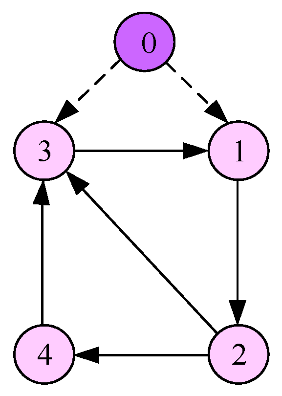
In order to verify the effectiveness of the proposed method, we considered a network containing delayed fractional-order multi-agents as shown in Figure 1, where the virtual leader and followers are numbered 0, 1, 2, 3, and 4, and the leader and followers are represented by dotted lines.

From Figure 1, the adjacency matrix $\mathit{M}$ and ${\mathit{D}}_{in}$ were

$$\mathit{M}=\left[\begin{array}{cccc}0& 0& 1& 0\\ 1& 0& 0& 0\\ 0& 1& 0& 1\\ 0& 1& 0& 0\end{array}\right],\mathit{D}=diag[\begin{array}{cccc}1& 1& 2& 1\end{array}]$$

Then the Laplacian matrix can be obtained as

$$\mathit{L}=\mathit{D}-\mathit{M}=\left[\begin{array}{cccc}1& 0& -1& 0\\ -1& 1& 0& 0\\ 0& -1& 2& -1\\ 0& -1& 0& 1\end{array}\right],\mathit{S}=diag[1,0,1,0]$$

In this paper, the fractional-order multi-agent with state delay can be described as follows

$$\left\{\begin{array}{l}{D}^{\alpha }{\mathit{x}}_j(t)=\left[\begin{array}{cc}0.4& 2\\ 5& -6\end{array}\right]{\mathit{x}}_j(t-h)+\left[\begin{array}{c}0\\ 1\end{array}\right]{\mathit{u}}_j(t),\\ {\mathit{y}}_j(t)=\left[0 1.2\right]{\mathit{x}}_j(t),\end{array}\right.$$

(37)

The expected trajectory of the multi-agent was $y_d(\mathrm{t})=2t^2+3t^3+\sin (2\pi t),t\in [0,1]$. In the simulation example, we set the fractional derivative α = 0.85, and the initial state and initial input of each iteration are 0 for all agents. That is ${\mathit{u}}_{0,j}(t)=0$, ${\mathit{x}}_{i,j}(0)=0$, and $j=1,2,3,4$.

• Case 1: Open-closed-loop PD^α-type

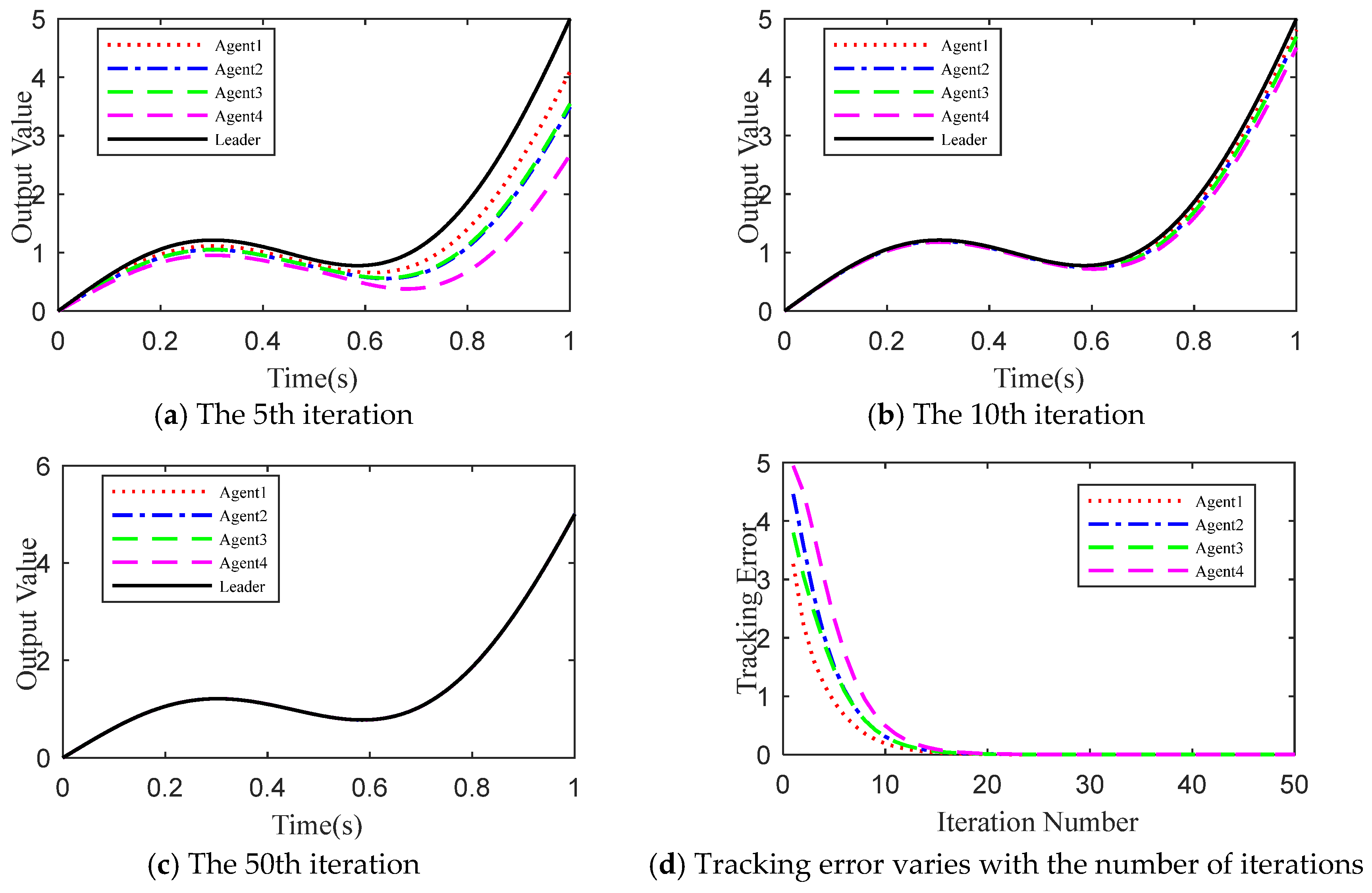
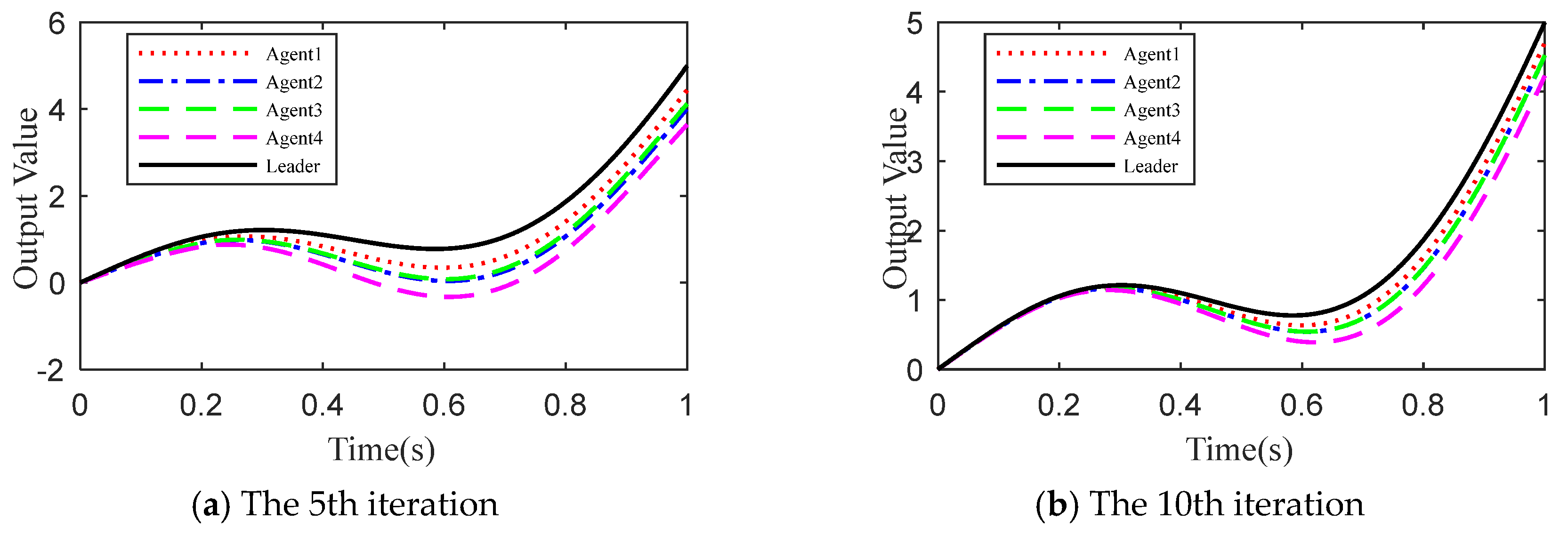
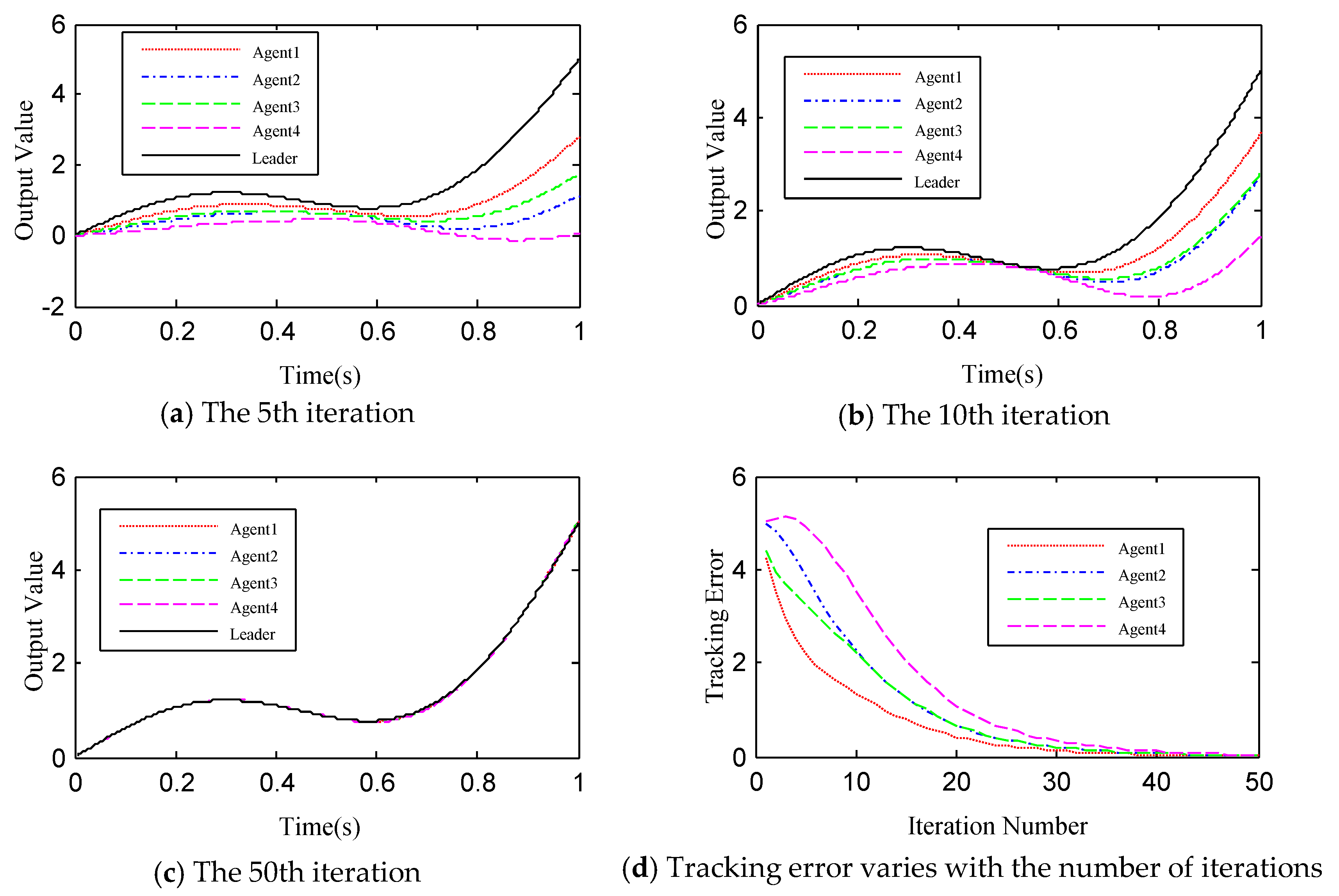
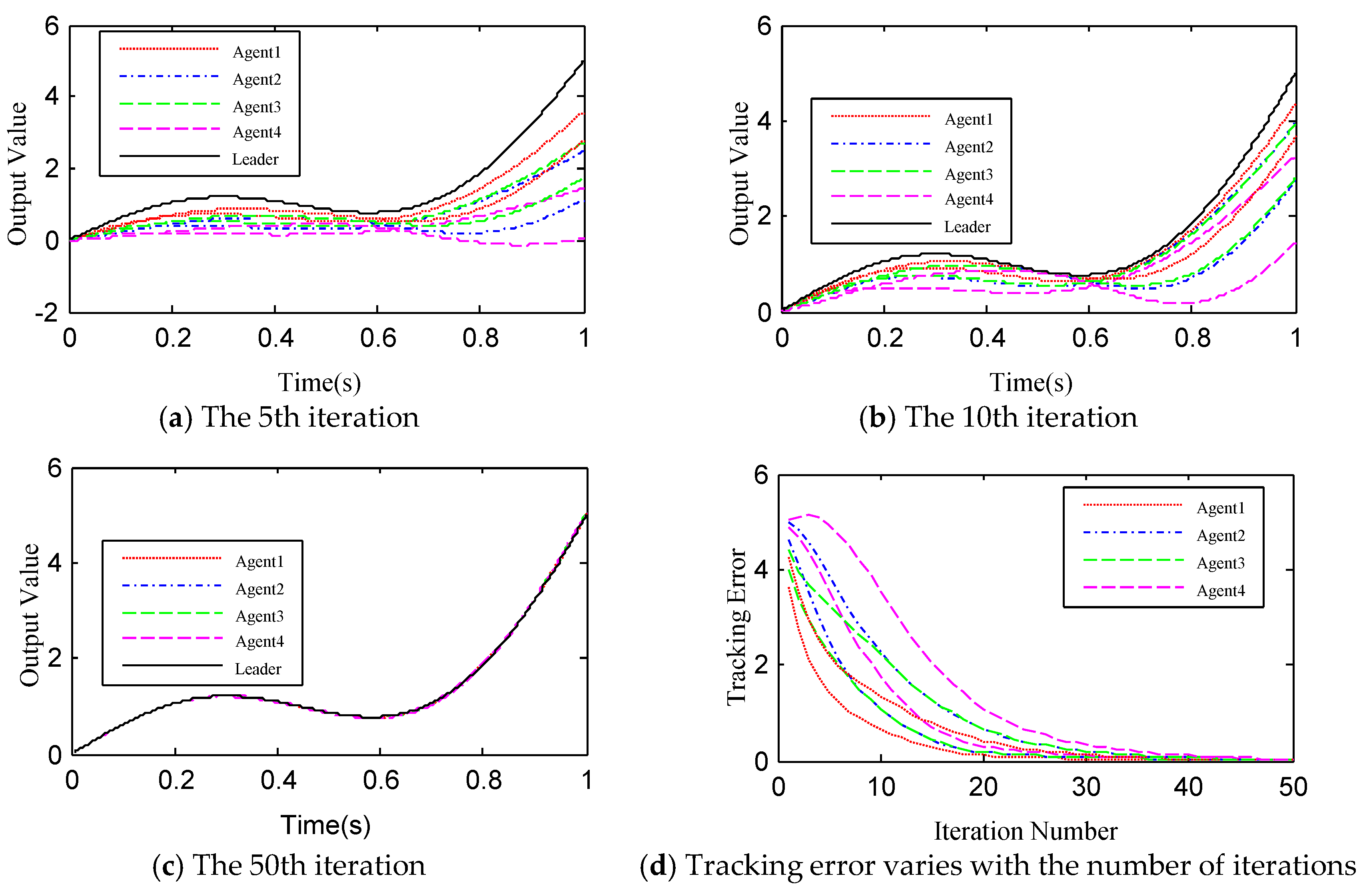
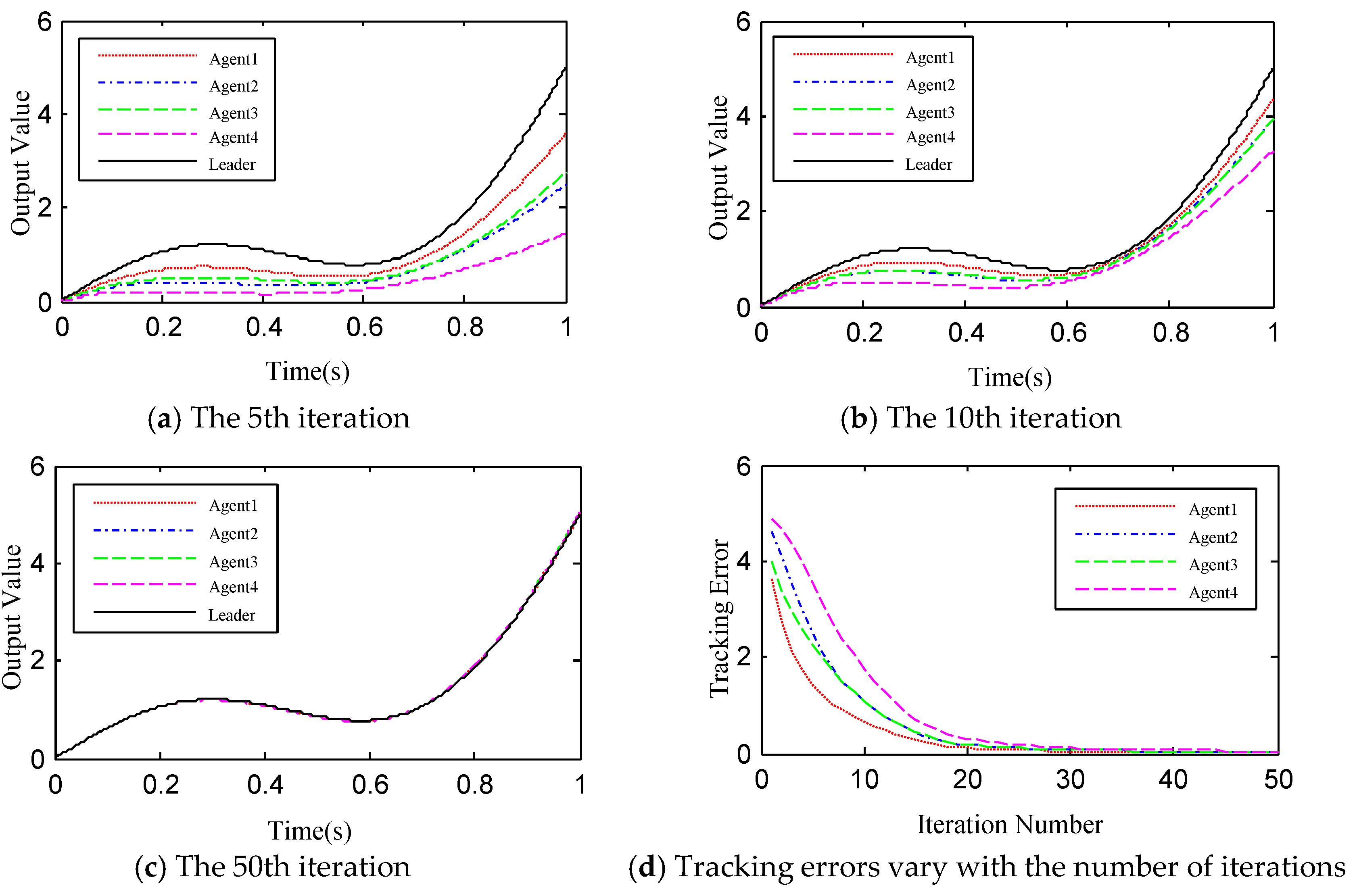
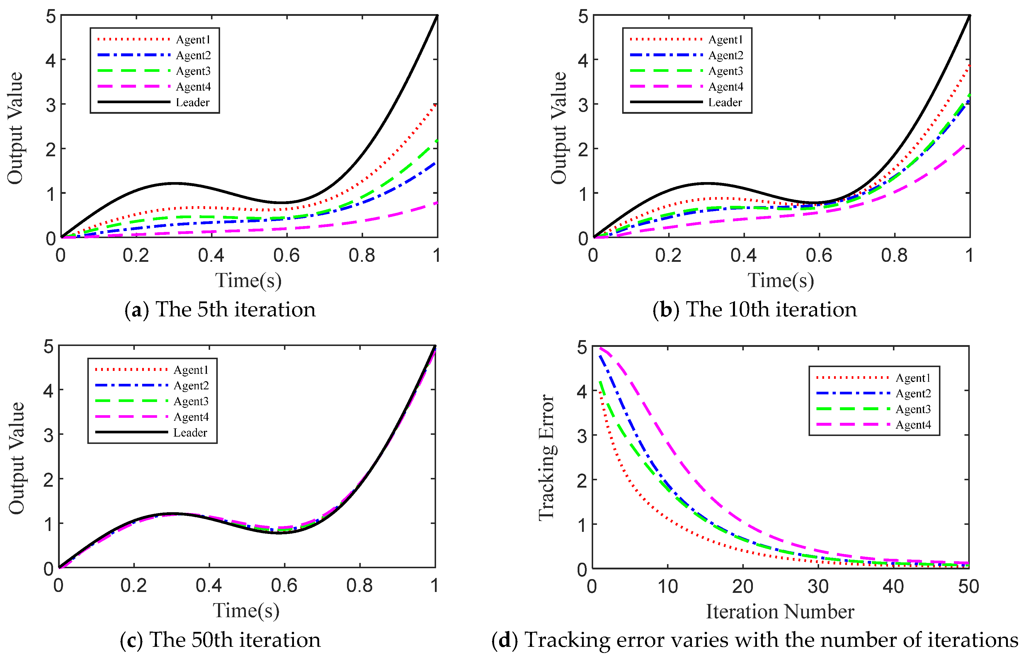
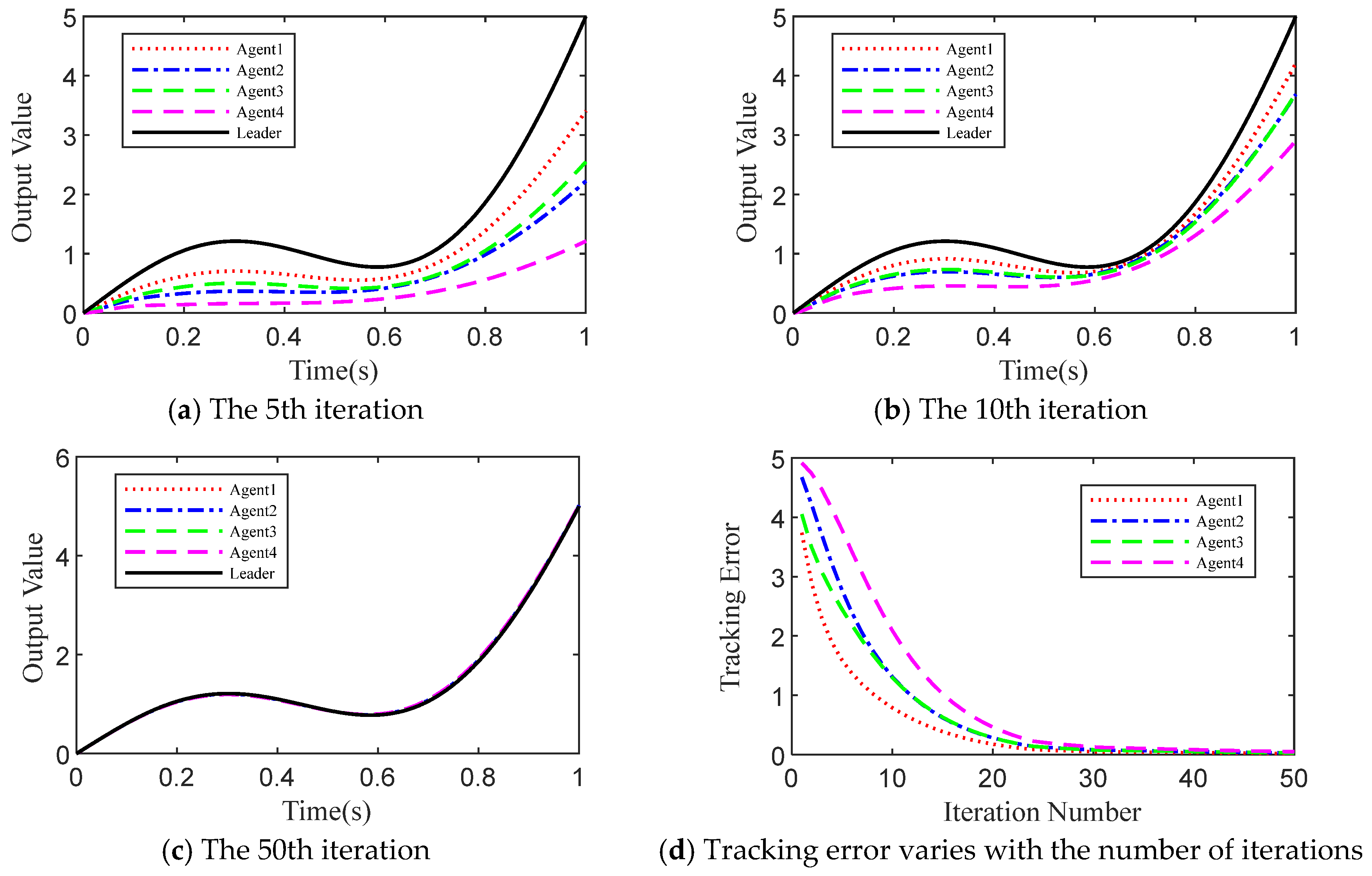
According to Theorem 1, we set the gain matrix to be ${\mathit{\Gamma }}_{P1}=1.2$, ${\mathit{\Gamma }}_{D1}=0.25$, ${\mathit{\Gamma }}_{P2}=1.6$, and ${\mathit{\Gamma }}_{D2}=1.1$. Thus, we obtained ${\rho }_1=0.876$ ${\rho }_2=0.963$, which satisfied the conditions in Theorem 1. In order to verify the effectiveness of the proposed method and the robustness to the delay time, the delay time was set to 0.1 and 0.5, or h = 0.1 and h = 0.5. The simulation results are shown in Figure 2 and Figure 3, which show the simulation results with the delay time of h = 0.1 and h = 0.5, respectively. Figure 2a, Figure 2b, and Figure 2c represent the tracking results of the 5th, 10th, and 50th iterations, respectively. Figure 2d shows the absolute value of the maximum errors in each iteration as the number of iterations changes. It can be seen from these results that as the number of iterations increased, each fractional-order multi-agent gradually tracked the desired trajectory. When h = 0.5, the maximum errors of the four followers were 0.0009, 0.0012, 0.0011, and 0.0015 at the fiftieth iteration, respectively. When compared with Figure 2, Figure 3 shows the tracking results where it can be seen that its convergence speed slowed down when h = 0.1 and the delay increased.

In addition, from the point of view of the convergence speed of each multi-agent, multi-agents 1 and 3 converged the fastest, while 2 and 4 converged slower. This is because multi-agents 1 and 3 could directly obtain information from the virtual leader.

• Case 2: Open-loop PD^α-type

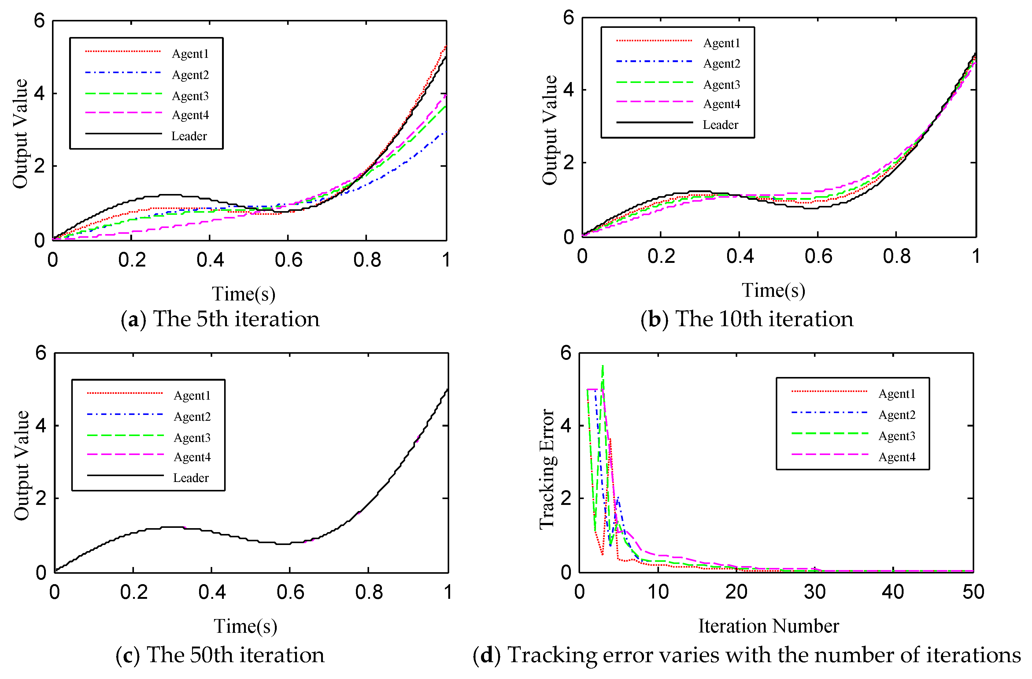
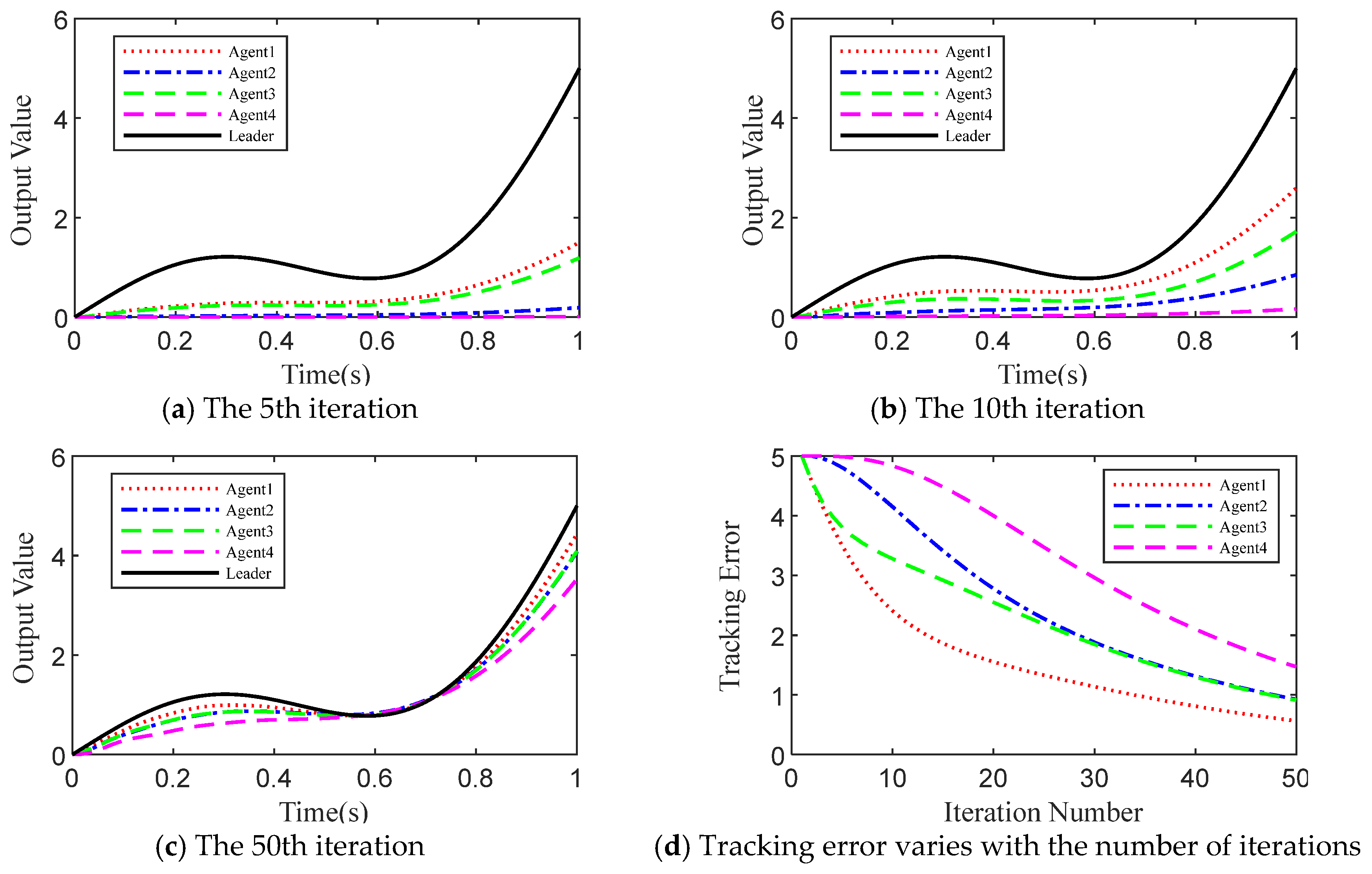
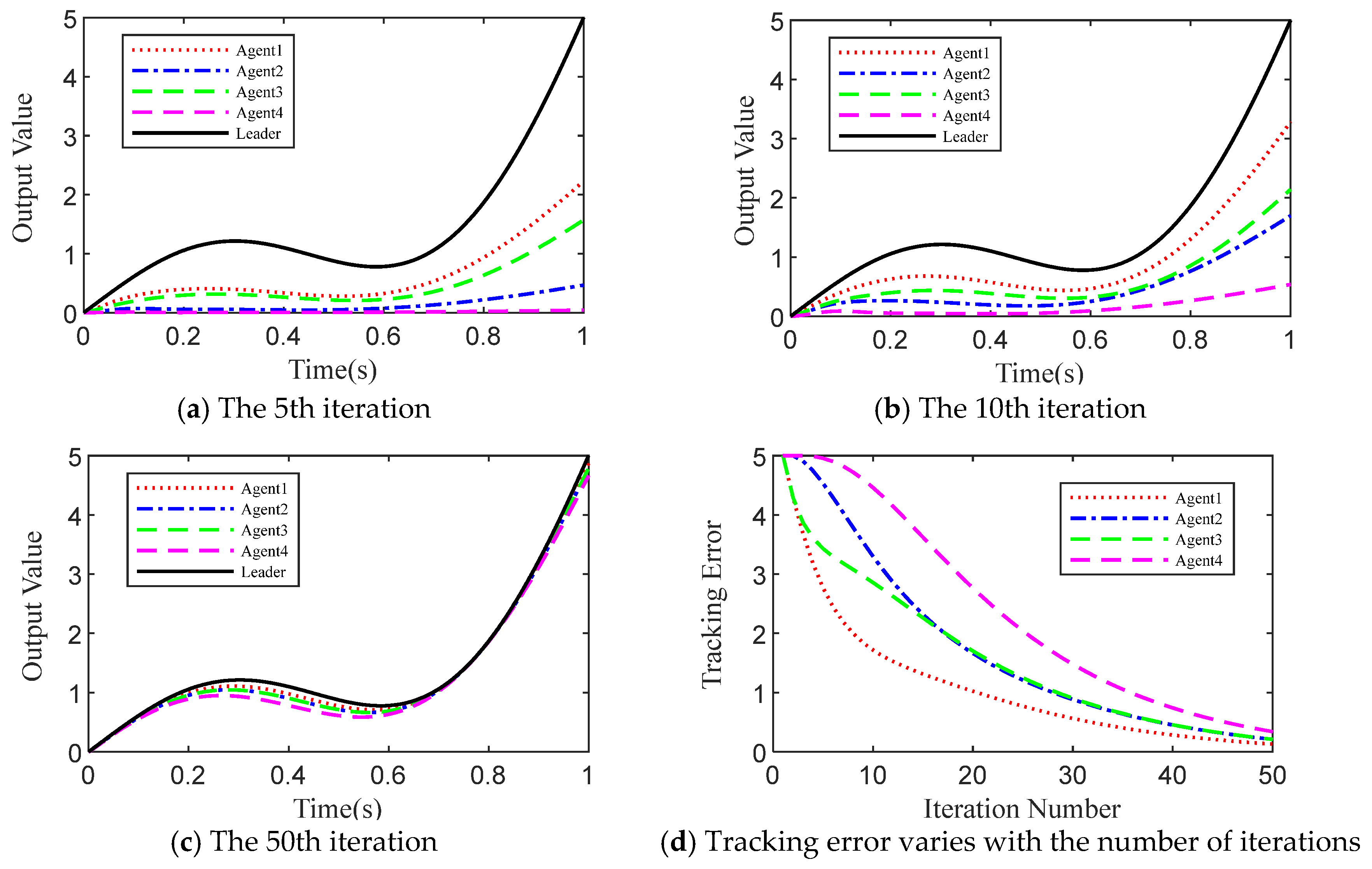
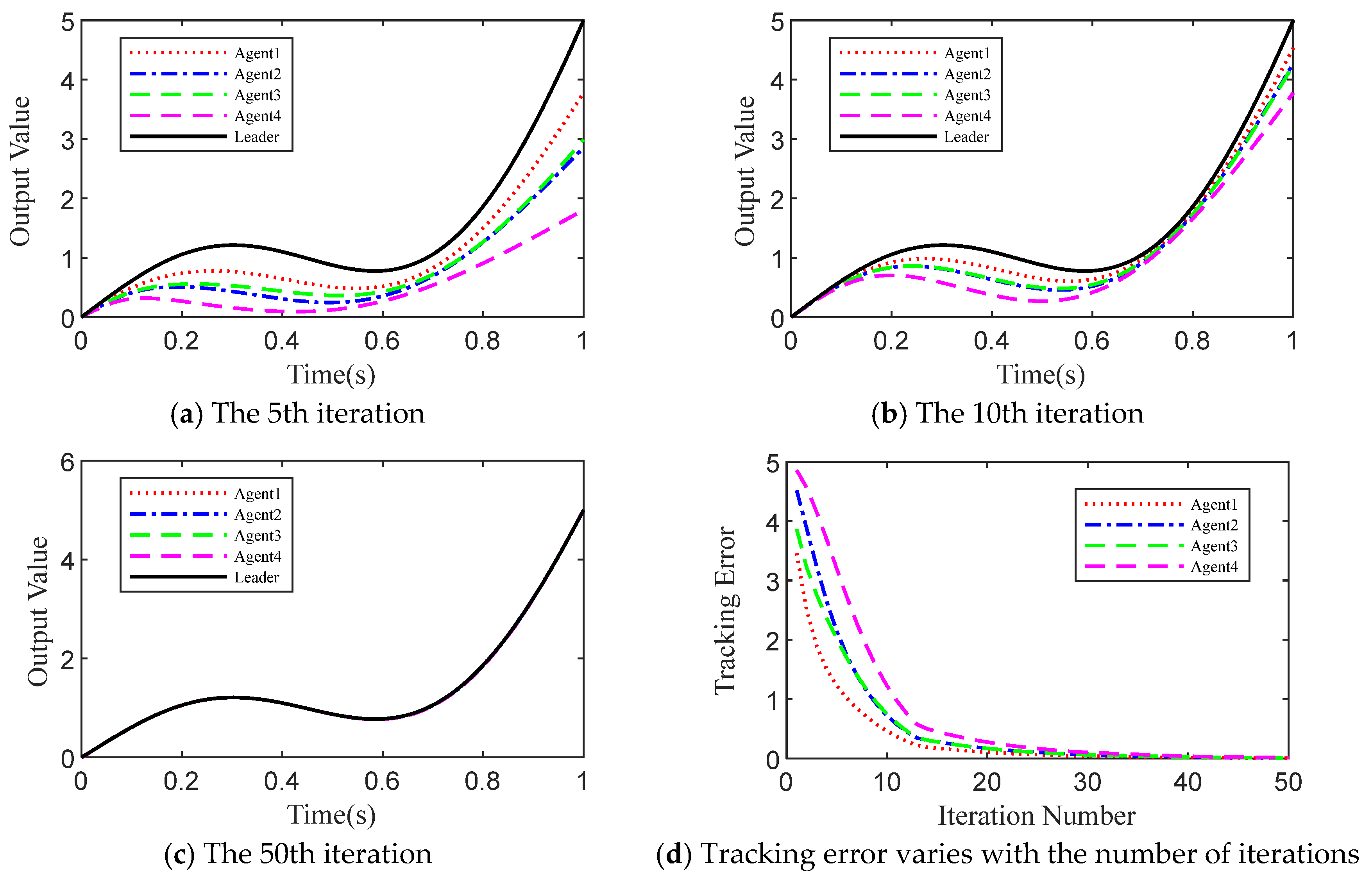
According to Corollary 1 and the controller in Equation (32), we set the gain matrix to be ${\mathit{\Gamma }}_{P1}=1.2$ and ${\mathit{\Gamma }}_{D1}=0.25$. Similarly to Case 1, the delay time is set to 0.1 and 0.5, or h = 0.1 and h = 0.5. The simulation results are shown in Figure 4 and Figure 5. Figure 4a and Figure 5a, Figure 4b and Figure 5b, and Figure 4c and Figure 5c represent the tracking results of the 5th, 10th, and 50th iterations, respectively. Figure 4d and Figure 5d show the absolute value of the maximum errors of each iteration as the number of iterations changes. As the number of iterations increased, the multi-agents gradually tracked the desired trajectory. When compared with the open-closed-loop PD^α-type FOILC under the same number of iterations, the control effect of the open-closed-loop PD^α-type FOILC was better than that of the open-loop PD^α-type FOILC. Thus, the introduction of closed-loop control in the open-closed-loop PDα-type FOILC improved the control performance and increased the convergence speed. In addition, it can be seen that the convergence speed slowed down when the delay increased.

• Case 3: Close-loop PD^α-type

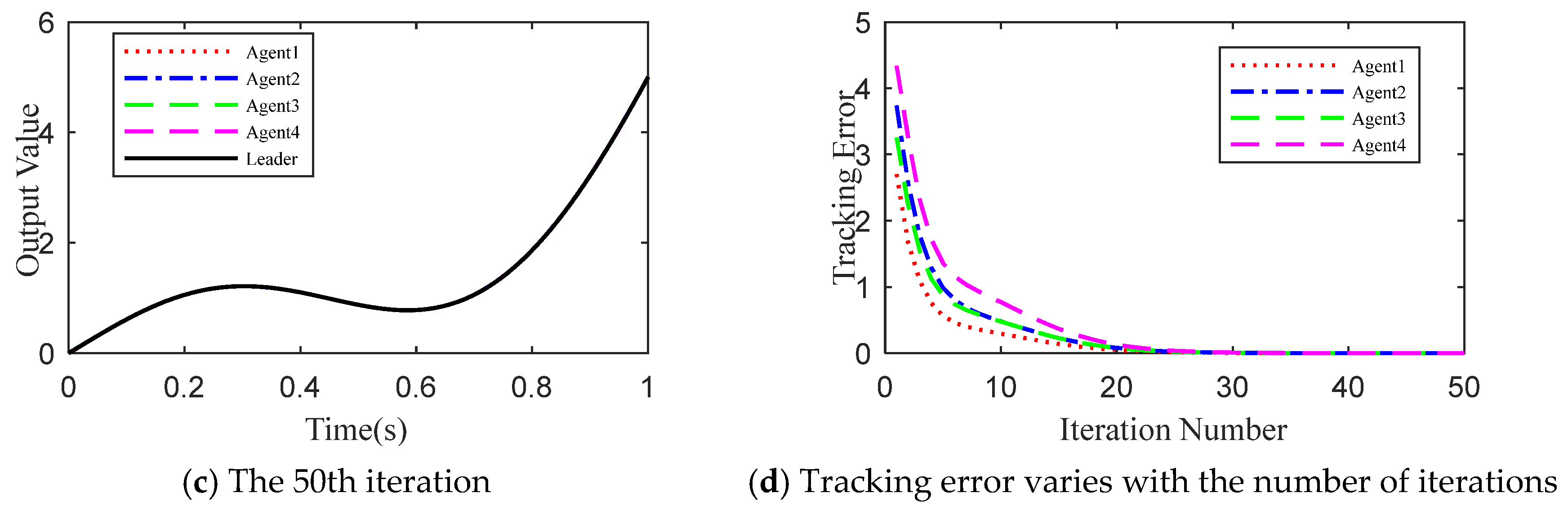
According to Corollary 2 and the controller in Equation (34), we set the gain matrix to be ${\mathit{\Gamma }}_{P2}=1.6$ and ${\mathit{\Gamma }}_{D2}=1.1$. Similar to the initial conditions in Case 1 and Case 2, the delay time was set to h = 0.1 and h = 0.5. When compared with the open-closed-loop PD^α-type FOILC and closed-loop PD^α-type FOILC, as shown in Figure 6 and Figure 7, we found that the close-loop PD^α-type FOILC has the slowest convergence speed.

• Case 4: Validation under mismatched orders between the controller and the plant model.

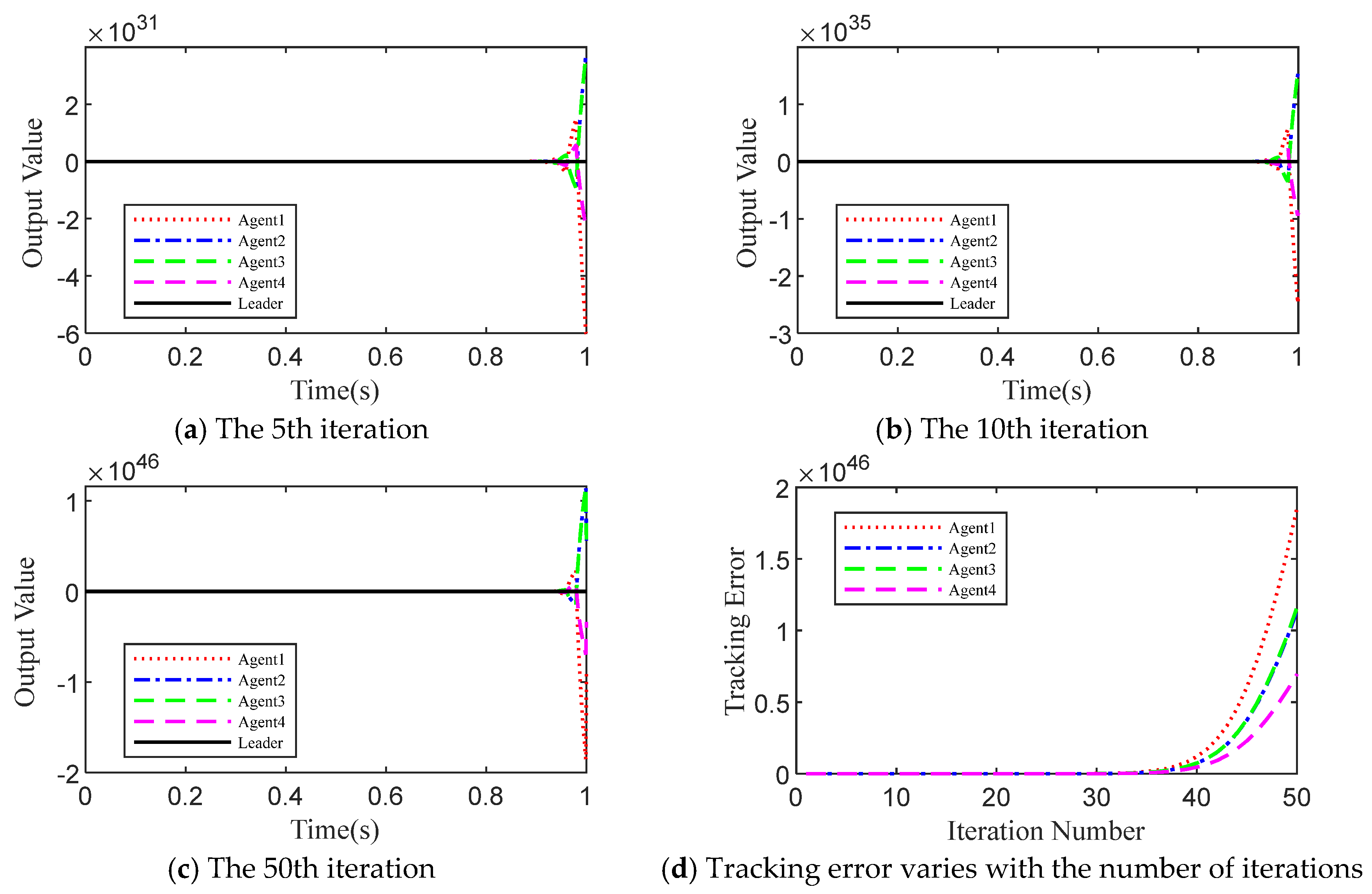
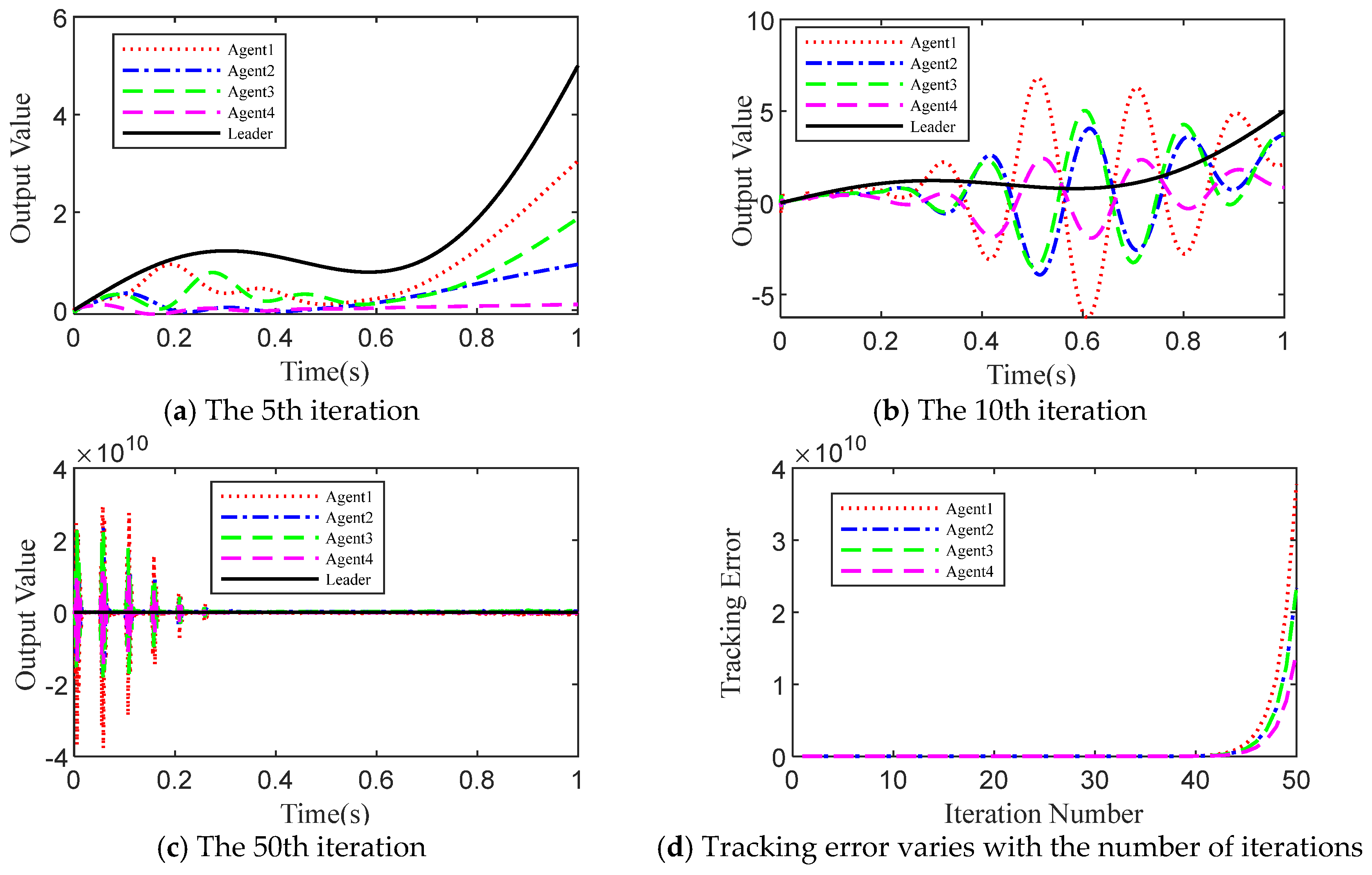
According to Corollary 1 and Corollary 2 in the paper, we conducted simulation verification on the convergence of the fractional-order open-loop iterative learning control and the closed-loop iterative learning control, respectively. In the simulations, the delay time was set to 0.1 s, i.e., h = 0.1. The control parameters for both open-loop and closed-loop schemes were kept consistent with those in the paper, i.e., ${\mathit{\Gamma }}_{P1}=1.2$ ${\mathit{\Gamma }}_{D1}=0.25$ ${\mathit{\Gamma }}_{P2}=1.6$ ${\mathit{\Gamma }}_{D2}=1.1$. By taking α as 0.2, 0.6, 0.95, and 1, respectively, we verified the convergence of the fractional-order multi-agent system under the fractional-order open-loop iterative learning control and the fractional-order closed-loop iterative learning control. The simulation results are shown in Figure 8, Figure 9, Figure 10, Figure 11, Figure 12, Figure 13, Figure 14 and Figure 15.

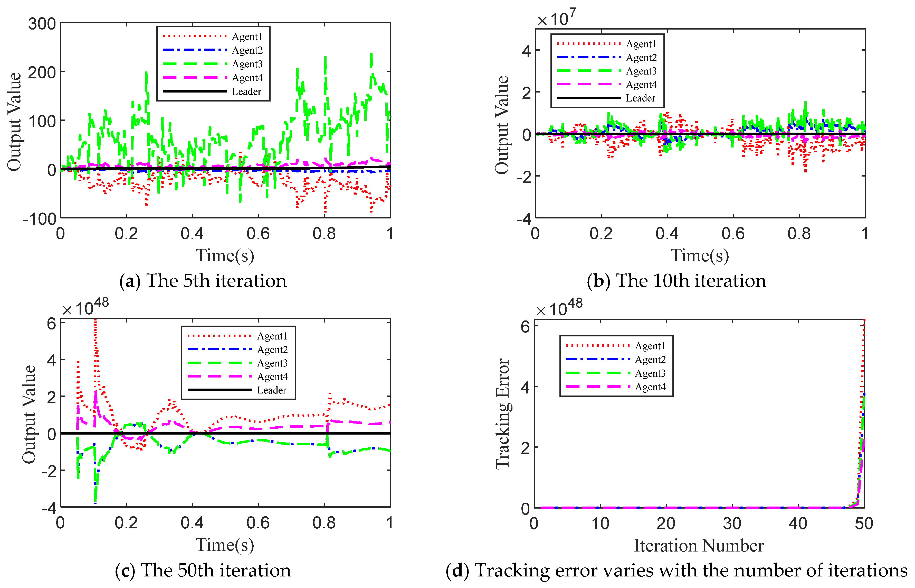
From the results of the fractional-order open-loop iterative learning control, it can be observed that when α = 0.2 and 0.95, the system failed to converge under the fractional-order open-loop iterative learning control strategy. For α = 0.4 and 0.6, although the fractional-order multi-agent system gradually converged, its convergence speed was noticeably slower compared with the control results for α = 0.85 under the same model and the same control law as discussed in the paper.

Regarding the simulation results under the fractional-order closed-loop iterative learning control, it can be seen that for different values of α, the fractional-order multi-agent system remained convergent in all cases. However, the convergence rate increased as α approached the system order of 0.85. Notably, when α = 1, the system failed to converge.

In nature, many actual physical systems have fractional-order dynamic characteristics, but the integer-order calculus theory that has been used is only a special case of the fractional-order calculus theory, which can only approximate the actual fractional-order system. However, the theory of fractional calculus can describe and reflect the nature of the object more truthfully and accurately, and through the fractional-order controller, the system can achieve better performance. Therefore, it is of great significance to the research results of this article.

5. Conclusions

This paper proposed a PDα open-closed-loop fractional-order iterative learning controller for fractional-order multi-agent systems with state delays. Based on norm theory, graph theory, and fractional calculus, the convergence properties of the proposed algorithm were rigorously analyzed, and sufficient convergence conditions were derived. Theoretical results demonstrate that, as the number of iterations increased, the tracking error of the fractional-order multi-agent system with state delays converged to zero. Finally, numerical simulations were conducted to verify the effectiveness of the proposed control method.