On a Friction Oscillator of Integer and Fractional Order; Stick–Slip Attractors

Abstract

This paper investigates a friction oscillator model in both its Integer-Order and Fractional-Order formulations. The lack of classical solutions for the governing differential equations with discontinuous right-hand sides is addressed by adopting a Differential Inclusion framework. Using Filippov regularization, the discontinuity is replaced by a set-valued map satisfying appropriate regularity conditions. Selection theory is then applied to construct a Lipschitz-continuous, single-valued function that approximates the set-valued map. This procedure reformulates the discontinuous initial value problem as a continuous, single-valued one, thereby providing a rigorous justification for the proposed approximation method. Numerical simulations are performed to study stick–slip attractors in both the Integer-Order and Fractional-Order cases. The results demonstrate that, in contrast to the Integer-Order system, periodic attractors cannot occur in the Fractional-Order regime.

1. Introduction

The phenomenon of stick–slip arises from the dynamic interaction between two contacting surfaces, which alternately adhere to each other and then slide relative to one another, resulting in fluctuations in the frictional force. In general, the force required to initiate motion (static friction) is greater than the force required to sustain motion (kinetic friction). Once the applied force exceeds the static friction threshold, the friction force drops to a lower kinetic value, leading to a sudden increase in sliding velocity. This behavior originates from the difference between static and kinetic friction coefficients and can produce complex and sometimes unpredictable dynamics in a wide range of systems [1,2,3,4].

Mechanical systems in contact with rough surfaces are inevitably influenced by frictional forces. Unlike viscous damping, which is continuous and proportional to velocity, dry friction is intrinsically nonlinear and discontinuous. This fundamental distinction gives rise to a variety of complex dynamical phenomena, including sliding modes, multiple equilibria, non-unique solutions at zero velocity, and, most notably, stick–slip motion. The repeated cycle of gradual energy accumulation followed by sudden release characteristic of stick–slip dynamics leads to non-smooth oscillations that are both practically significant and mathematically challenging [5,6].

From a theoretical standpoint, stick–slip dynamics belong to the class of non-smooth dynamical systems [7,8]. The governing equations are typically defined in a piecewise manner, with discontinuities in the vector field across specific manifolds, such as the zero-velocity surface. As a result, classical smooth dynamical systems theory is no longer directly applicable. Various analytical approaches have been proposed to address this difficulty, ranging from Filippov’s theory of differential inclusions, which rigorously treats genuine discontinuities [9], to regularized friction laws that smooth the transition between sticking and slipping regimes [10,11]. Both approaches aim to capture the essential feature of frictional systems: abrupt switching of forces when critical thresholds are reached.

Many physical systems encountered in engineering and applied mathematics exhibit discontinuous right-hand sides in their dynamical descriptions. Such discontinuities naturally arise in systems involving friction, impacts, switching control laws, relays, and phase transitions [7]. Filippov regularization [9] provides a powerful and mathematically consistent framework for analyzing these systems. By reformulating discontinuous differential equations as differential inclusions with well-defined set-valued maps, it enables the application of advanced tools from non-smooth analysis to problems that are ubiquitous in engineering and the natural sciences. This framework has been successfully applied in numerous fields, including mechanical systems with friction [10], electrical circuits [12], control theory [13], biological systems [14], and power systems [15].

Fractional Differential Equations (FDEs) constitute a significant generalization of classical ordinary differential equations by extending the concept of differentiation to non-integer orders. Over the past decades, this mathematical framework has attracted considerable attention due to its ability to model complex physical processes exhibiting memory effects, hereditary properties, and long-range temporal dependencies [16,17]. Unlike integer-order derivatives, which describe purely local behavior, fractional derivatives incorporate the entire history of the system, making them especially suitable for modeling anomalous diffusion, viscoelastic materials, and biological systems characterized by power-law memory kernels.

Among the various definitions of fractional derivatives, the Caputo derivative adopted in this paper is particularly advantageous for initial value problems (IVPs) in applied mathematics and engineering. In this formulation, initial conditions are specified in terms of standard integer-order derivatives, which aligns naturally with physical interpretations and experimental measurements. Caputo fractional differential equations have found widespread applications across diverse scientific domains, including viscoelasticity [18], anomalous diffusion [19], control systems [20], and biological systems [21].

In engineering applications—such as aircraft control systems, power grids, and digital circuits—the presence of hidden attractors can lead to unexpected and potentially catastrophic bifurcations. A system may appear stable under standard operating conditions, yet a sufficiently large external perturbation can drive it into the basin of attraction of a hidden, undesirable attractor, such as a large-amplitude oscillation, resulting in system failure. The study of hidden attractors is particularly relevant for fractional-order systems, where the non-local, memory-dependent nature of fractional derivatives can significantly alter the system dynamics [22].

While self-excited attractors can be revealed by selecting initial conditions in the vicinity of unstable equilibria (e.g., saddle points), hidden attractors cannot be detected using this approach. Their basins of attraction are not connected to any equilibrium point, which makes them notoriously difficult to locate numerically. Identifying hidden attractors typically requires carefully chosen initial conditions, often obtained through specialized analytical or numerical techniques, located far from known equilibria. Hidden attractors may occur in systems with no equilibria, systems possessing only stable equilibria, systems whose basins are disconnected from equilibria even when unstable equilibria exist, or systems with a continuum (line) of equilibria [22].

The remainder of this paper is organized as follows. Section 2 introduces the friction oscillator model. Section 3 addresses the existence, uniqueness, and numerical integration of solutions to the underlying initial value problem. In Section 4, the stick–slip phenomenon is analyzed both theoretically and numerically. Section 5 is devoted to the fractional-order friction oscillator. Finally, the paper concludes with the Conclusion.

2. Friction Oscillator

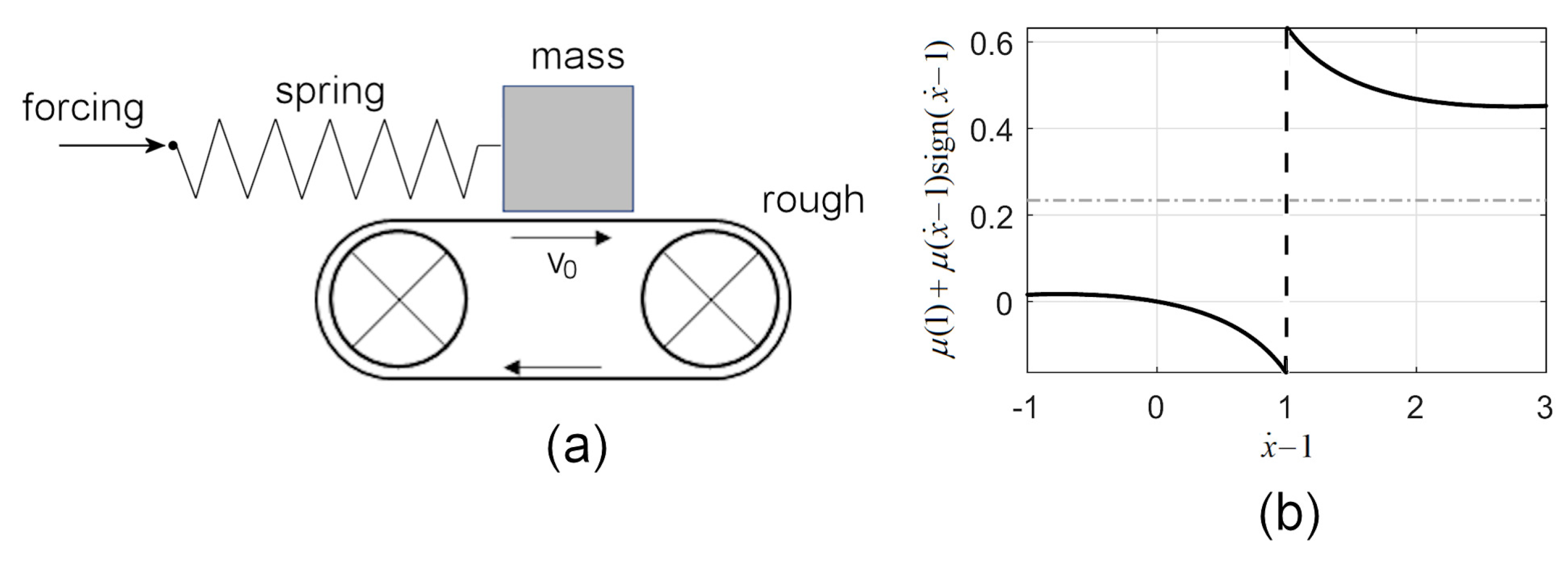
The friction oscillator considered in this work [4,23] consists of a mass attached to a linear spring resting on a moving rough belt and subjected to an external periodic excitation. The motion of the belt generates a friction force that opposes the relative velocity between the block and the belt (see Figure 1a).

The dynamics of the system are governed by

$$\ddot{x}+x+a\left[\mu \left(1\right)+\mu (\dot{x}-1),sign(\dot{x}-1)\right]=\gamma cos\left(\eta t\right).$$

(1)

The nonlinearity and discontinuity of the model arise from the term $\mu (\dot{x}-1)sign(\dot{x}-1)$, while the forcing term $\gamma cos\left(\eta t\right)$ renders the system non-autonomous.

The nonlinear friction characteristic $\mu :\mathbb{R}\to \mathbb{R}$ is an even function defined by

$$\mu \left(v\right)={\displaystyle \frac{{\mu }_0-{\mu }_1}{1+{\lambda }_0\left|v\right|}}+{\mu }_1+{\lambda }_1{\left|v\right|}^2,$$

(2)

for $v\in \mathbb{R}$, where $v=\dot{x}-v_0$ denotes the relative velocity and $v_0=1$ is the normalized belt speed.

The set of the parameters considered are nonnegative

$$\mathcal{P}:{\mu }_0=0.4, {\mu }_1=0.1, {\lambda }_0=1.42, {\lambda }_1=0.01.$$

(3)

$\eta$ is considered the bifurcation parameters and, unless specified, $a=10$ and $\gamma =1.15$. For the parameters $\mathcal{P}$, ${\mu }_1\ne \mu \left(1\right)\approx 0.234$, while $\mu \left(0\right)={\mu }_0=0.4$ (as considered in [4]).

The components of the model represent:

-

$\ddot{x}$: The inertial term (mass × acceleration);

-

x: The displacement. Note that $-x$ represents the restoring force from a linear spring, with its coefficient of 1 (stiffness 1) representing implicitly the spring constant. This force pulls the mass back toward its resting position. It stores and releases energy.

-

$\gamma cos\left(\eta t\right)$: The external excitation force;

-

$a[\mu \left(1\right)+\mu (\dot{x}-1)sign(\dot{x}-1)]$: The nonlinear asymmetric friction force about the origin (see Figure 1b for parameters $\mathcal{P}$, given by (3)), where:

-

$(\dot{x}\left(t\right)-1)$: The relative velocity between the block and the moving belt;

-

$\mu \left(v\right)$: The velocity-dependent friction coefficient. It typically has high static friction (${\mu }_0$) and lower kinetic friction (${\mu }_1$);

-

$\mu \left(1\right)$: A constant offset. It creates different static friction thresholds for positive and negative slip, making the friction force asymmetric.

The analytical model (1) can be expressed in the following autonomous form:

$$\begin{array}{c}{\dot{x}}_1=x_2,\hfill \\ {\dot{x}}_2=-x_1-a(\mu \left(1\right)+\mu (x_2-1)sign(x_2-1))+\gamma cos\left(\varphi \right),\hfill \\ \dot{\varphi }=\eta \hfill \end{array}$$

with $\varphi =\eta ·t$. With the substitution

$$v=x_2-1,$$

(4)

adapted to a belt speed of 1, the shift $x_2-1$ is “absorbed” into the new state v

$$\begin{array}{c}{\dot{x}}_1=v+1,\hfill \\ \dot{v}=-x_1-a(\mu \left(1\right)+\mu \left(v\right)sign\left(v\right))+\gamma cos\left(\varphi \right), x\left(0\right)=x_0,\hfill \\ \dot{\varphi }=\eta \hfill \end{array}$$

(5)

that represents the IVP modeling of the system in the space $(x_1,v,\varphi )$, with $x_0=(x_{10},v_0,{\varphi }_0)$.

The form (5) is useful both for the analytical approach (existence and uniqueness of solutions) and also for the numerical approach.

Remark 1. 

The velocity variable is shifted according to (4), namely $v=x_2-1$, where $x_2$ denotes the physical velocity of the system. This shift explains the appearance of the term $v+1$ on the right-hand side (RHS) of system (5). Consequently, all numerical simulations (time histories and phase portraits) are presented in terms of the shifted velocity variable v, while the physical velocity is recovered as $x_2=v+1$ (see also the horizontal axis labeled $\dot{x}-1$ in Figure 1b).

Although this transformation modifies the direct correspondence with the physical velocity, it allows the system to be expressed in a form that is more amenable to rigorous mathematical analysis. In particular, it facilitates the study of existence and uniqueness of solutions and provides a convenient framework for approximating and regularizing the system discontinuity. This formulation represents a compromise between preserving physical interpretability and achieving analytical and numerical tractability. Importantly, all stability properties and qualitative behaviors investigated in this paper are preserved under this coordinate transformation.

3. Solutions of the System (5)

3.1. Existence of the Solutions

Discontinuous autonomous problems, like the considered friction oscillator, can be modeled by IVPs for an autonomous ODE where the RHS function is piecewise continuous, discontinuous with the state variable, and continuous in the independent variable, t

$$\dot{x}=f\left(x\right), x\left(0\right)=x_0, t\in I=[0,\infty ).$$

(6)

$f:{\mathbb{R}}^n\to {\mathbb{R}}^n$ is a continuous function on ${\mathbb{R}}^n\setminus \mathcal{M}$, $\mathcal{M}$ being the discontinuity set of f of zero measure [24].

As is known, for these problems, the standard existence and uniqueness theorems cannot apply because they require f to be at least continuous in x. Therefore, a solution in the classical sense (a differentiable function $x\left(t\right)$) satisfying the ODE everywhere) might not exist. Moreover, if a solution exists, it might not be unique.

Consider the following example [25]:

$$\dot{x}=2-3sign\left(x\right), x\left(0\right)=x_0,$$

(7)

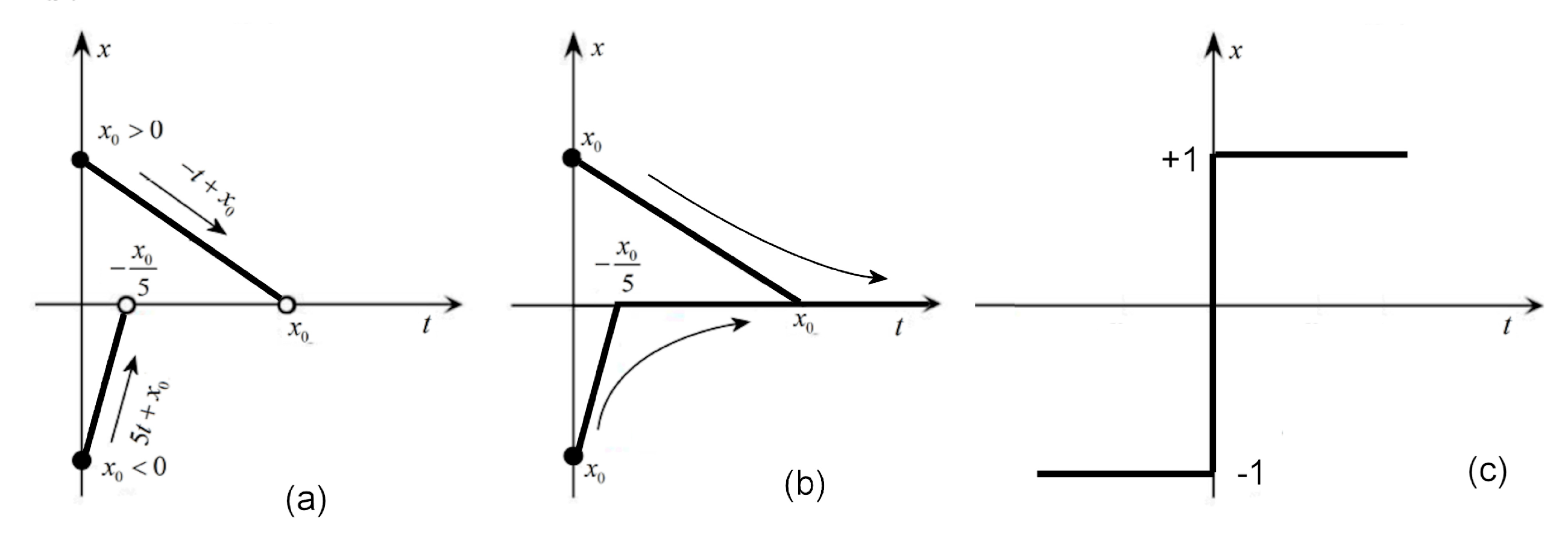
where $f:\mathbb{R}\to \mathbb{R}$ is continuous for $x\in (-\infty ,0)\bigcup (0,\infty )$ and discontinuous at $x=0$ ($\mathcal{M}=\left\{0\right\}$). If $x_0>0$, the solution $x\left(t\right)=x_0-t$ decreases linearly to the axis $x=0$ for $t<t_{\ast }=x_0$. If $x_0<0$, the solution $x\left(t\right)=x_0+5t$ also tends to $x=0$ for $t<t_{\ast }=-x_0/5$. Therefore, every solution with $x_0\ne 0$ tends to $x=0$ but for finite time and cannot be prolonged along this axis. The reason is that for $x_0=0$, the equation has no sense since by replacing $x=0$ in the equation, one obtains $\dot{0}=2-sign\left(0\right)$; therefore, the definition of the standard solution is not verified (Figure 2a).

A possible approach to overcome this obstacle is to regularize the problem by restarting it as a Differential Inclusion (DI).

$$\dot{x}\in F\left(x\right), x\left(0\right)=x_0, \mathrm{for} \mathrm{a}.\mathrm{e}. t\in I,$$

(8)

where $F:{\mathbb{R}}^n\rightrightarrows \mathcal{P}\left({\mathbb{R}}^n\right)$ is a set-valued function into the family of all nonempty subsets of ${\mathbb{R}}^n,\mathcal{P}\left({\mathbb{R}}^n\right)$. The common way to define F is defined by the so-called Filippov regularization [9].

$$F\left(x\right)=\bigcap _{\epsilon >0}\overline{conv\left(f\left(\{z\in {\mathbb{R}}^n:\parallel z-x\parallel \le \epsilon \}\setminus \mathcal{M}\right)\right)}.$$

(9)

An important property of the set-valued function F defined by (9) is that the set $F\left(x\right)$ represents the closure of the convex hull of f, with $\epsilon$ representing the radius of the ball centered at x. At x, where f is continuous, $F\left(x\right)$ is a point $F\left(x\right)=\left\{f\right(x\left)\right\}$, while at the points of discontinuity, $F\left(x\right)$ is the set given by (9).

F defined by Filippov regularization is Upper Semicontinuous (USC) [26,27].

The Filippov regularization of the discontinuous function curve $sign\left(x\right)$, S-shaped, and denoted $Sign\left(x\right)$, also called sometimes “sigmoid” function is (Figure 2c).

$$Sign\left(x\right)=\left\{\begin{array}{cc}\{+1\}\hfill & x>0,\hfill \\ [-1,1]& x=0,\hfill \\ \{-1\}\hfill & x<0,\hfill \end{array}\right.$$

i.e., a set-valued function which is identical to the function $sign\left(x\right)$, for $x\ne 0$, but at $x=0$ replaces the zero value, with the set $[-1,1]$.

In this way, the discontinuous initial value problem (IVP) (6) is reformulated as the set-valued IVP (8), which, due to the regularization (9), admits solutions known as Filippov (generalized) solutions.

Applying Filippov regularization, the IVP (5) is transformed into the following set-valued IVP:

$$\begin{array}{c}{\dot{x}}_1=v+1,\hfill \\ \dot{v}\in -x_1-a(\mu \left(1\right)+\mu \left(v\right)Sign\left(v\right))+\gamma cos\left(\varphi \right), x\left(0\right)=x_0, \mathrm{for} \mathrm{a}.\mathrm{e}. t\in I,\hfill \\ \dot{\varphi }=\eta .\hfill \end{array}$$

(10)

In (10), at the discontinuity $v=0$, the set-valued map of the term $\mu \left(v\right)Sign\left(v\right)$ is the convex hull of the one-sided limits of

$$\mathrm{conv}\{\underset{v\to 0_{-}}{lim}\mu \left(v\right)sign\left(v\right),\underset{v\to 0_{+}}{lim}\mu \left(v\right)sign\left(v\right)\}=[-\mu \left(0\right),+\mu \left(0\right)].$$

Definition 1. 

A generalized (Filippov) solution to the set-valued IVP (8) is an absolutely continuous vector-valued function $x:I\to R^n$ satisfying (8) for a.e. $t\in I$.

Remark 2. 

(i)    Set-valued functions admit a natural interpretation in terms of their graphs; consequently, a set-valued function is said to satisfy a given property if and only if its graph satisfies the corresponding property [26]. For instance, a set-valued function is closed if and only if its graph is closed. In practical applications, it is often more convenient to consider the closure of the graph of F rather than the closedness of its values.

(ii)     

By embedding the discontinuous vector field f into a suitably regular set-valued map F, any classical solution of the underlying discontinuous IVP (6) is also a solution of the set-valued IVP (8). It is therefore justified to regard any solution of the discontinuous problem (6) as a solution of the IVP (8).

Theorem 1 (Existence). 

Let there be a discontinuous IVP (6) with f locally bounded. Then, the corresponding IVP (8), with F defined by the Filippov regularization (9), admits at least one generalized solution.

Proof. 

If f is locally bounded, F is a Péano function, i.e., it is an USC function, non-empty, closed, and convex (Remark 2i)) [25].    □

Note that ODEs with discontinuous RHS with discontinuity due to sign-like functions are locally bounded and, therefore, the following result holds.

Proposition 1. 

The IVP (5) admits at least a generalized solution.

By using the regularization to Example (7), one obtains the following problem:

$$\dot{x}\in 2-3Sign\left(x\right)=\left\{\begin{array}{cc}\{-1\}\hfill & x>0,\hfill \\ [-1,5]\hfill & x=0, x\left(0\right)=x_0.\hfill \\ \{+5\}\hfill & x<0.\hfill \end{array}\right.$$

From Theorem 1, the problem admits a positive generalized solution $x\left(t\right)=-t+x_0$ for $t<x_0$ and $x\left(t\right)=0$ for $t\ge x_0$ so that the solution can now be continuously prolonged after it crosses the axis $x=0$. Similarly, there is a negative solution for $x_0<0,x\left(t\right)=5t+x_0$ for $t<x_0$ and $x\left(t\right)=0$ for $t\ge x_0$. Now, at $x_0=0$, the set-valued Sign function generates the set $[-1,5]$, within which one can choose any value (Figure 2b).

3.2. Numerical Integration

The set-valued formulation of the underlying discontinuous problem provides only a characterization of generalized solutions and does not, by itself, furnish a practical procedure for their numerical computation.

In general, numerical methods for differential inclusions (DIs) differ substantially from those used for ordinary differential equations (ODEs) (see, e.g., [28,29]). For instance, the system may be integrated using standard ODE solvers as long as the state satisfies $x\notin \mathcal{M}$. When the trajectory enters a sufficiently small neighborhood of the discontinuity surface $\mathcal{M}$, one may, for example, select a value for the derivative from the set $F\left(x\right)$, possibly at random. The solution segments obtained before and after crossing the discontinuity manifold can then be “glued” together.

However, one of the simplest and most effective approaches to handling the set-valued problem (8)—and the one adopted in this work, in line with known approximation results—is to transform the set-valued initial value problem into a continuous, single-valued one. This reformulation allows the system to be treated numerically as a continuous ODE, which can then be integrated using standard numerical techniques.

Definition 2. 

The single-valued function $f:{\mathbb{R}}^n\to {\mathbb{R}}^n$ is called a selection (approximation) of the set-valued function F if satisfies $f\left(x\right)\in F\left(x\right)$ for $x\in {\mathbb{R}}^n$.

One of the possibilities to approximate the set-valued IVP (8) with a single-valued continuous IVP is the Cellina Theorem, which ensures the existence of the approximate continuous selection.

Theorem 2 

([26]). For the set-valued function F defined with the Filippov regularization, and every $\epsilon >0$, there exists a locally Lipschitz selection $f_{\epsilon }:{\mathbb{R}}^n\to {\mathbb{R}}^n$ such that

$$Graph\left(f_{\epsilon }\right)\subset Graph\left(F\right)+\epsilon B,$$

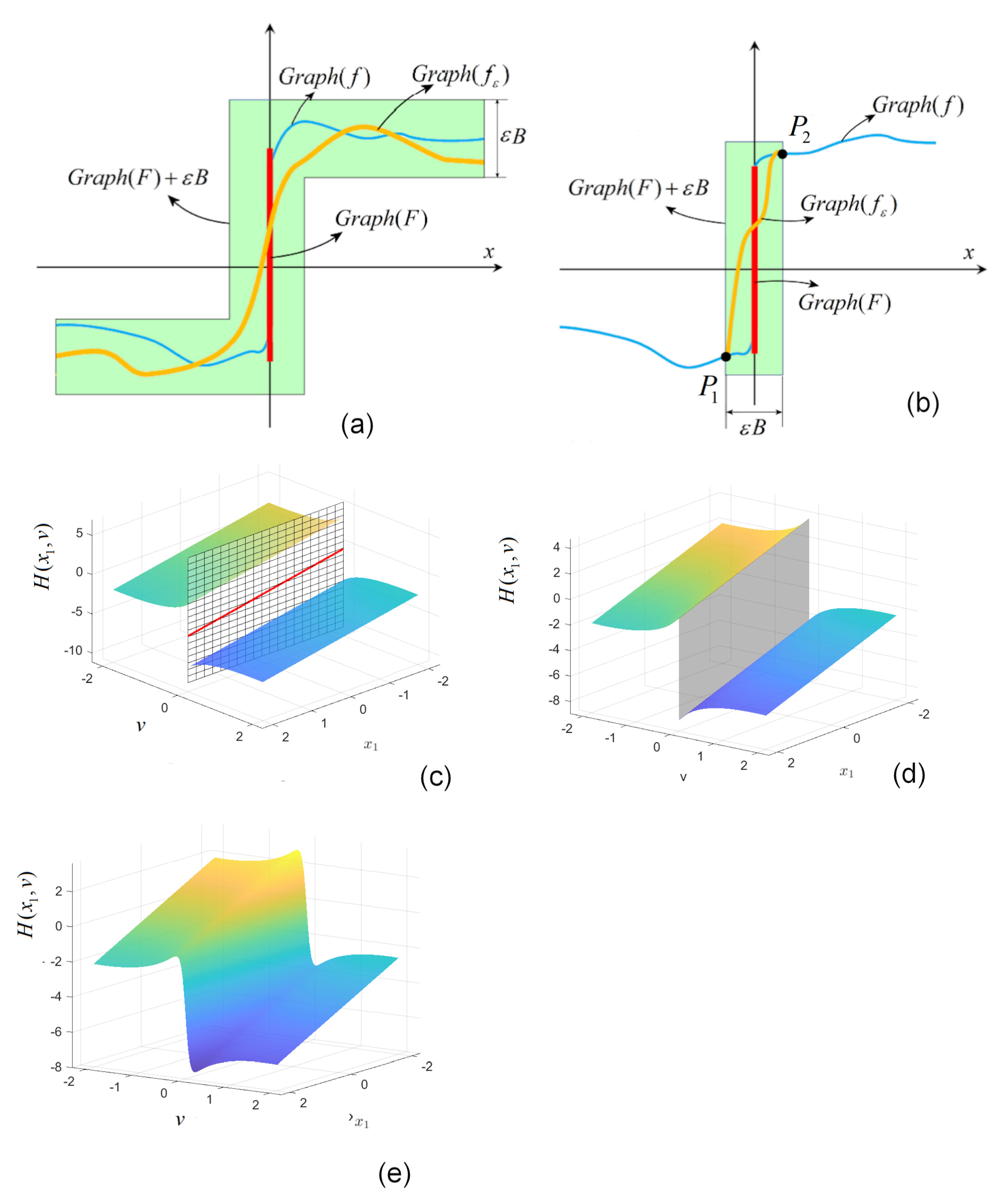
where B is the unit ball in ${\mathbb{R}}^n$ centered in a point of $Graph\left(F\right)$ (Figure 3a).

There are several Lipschitz continuous single-valued approximations of the one-dimensional set-valued functions $Sign\left(x\right)$ considered in this paper and denoted as ${sign}_{\epsilon }\left(x\right)$, such as

$${\displaystyle \frac{2}{\pi }}arctan{\displaystyle \frac{x}{\delta }}, {\displaystyle \frac{x}{x^2+\delta }}, {\displaystyle \frac{2}{1+e^{\frac{x}{\delta }}}}.$$

(11)

Note that in Approximations (11), the subscript $\epsilon$ indicates the neighborhood within the approximation is done, with $\delta$ being the parameter giving the slope of the approximation. $\delta$ and $\epsilon$ are parameters that are interdependent. Usually, $\epsilon$ is determined by the choice of $\delta$.

The set-valued function $Sign\left(x\right)$ is approximated by

$${sign}_{\epsilon }\left(x\right)=tanh{\displaystyle \frac{x}{\delta }},$$

(12)

with $\delta =1/900$. Although this value represents a relative aggressive smoothing parameter, it approaches better the discontinuity.

Remark 3. 

All approximations presented above are global so that they approximate the RHS of the underlying problem along the entire domain (see the sketch in Figure 3a). On the other side, local approximations, which apply only locally on small neighborhoods of the discontinuity $x=0$ (curve $P_1{P}_2$ in the neighborhood $\epsilon B$ in Figure 3b) are better approximations than the global approximations, but at the expense of computation time (see [25]).

The main result of this section is as follows.

Theorem 3. 

The numerical solutions to the discontinuous IVP (5) can be obtained by solving the following continuous IVP:

$$\dot{x}=f_{\epsilon }\left(x\right), x\left(0\right)=x_0,$$

(13)

where

$$f_{\epsilon }\left(x\right):=f_{\epsilon }(x_1,v,\varphi )=\left(\begin{array}{c}v+1\\ -x_1-a[\mu \left(1\right)+\mu \left(v\right){sign}_{\epsilon }\left(v\right)]+\gamma cos\left(\varphi \right)\\ \eta \end{array}\right).$$

Let $\gamma =0$. Then, the second component of System (13)

$$H(x_1,v)=-x_1-a[\mu \left(1\right)+\mu \left(v\right)sign\left(v\right)]$$

(14)

can be visualized before and after regularization and approximation (with $\delta =100$ for a clear visualization) in Figure 3c–e, respectively.

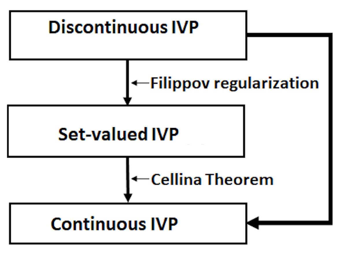
The algorithm of transforming the discontinuous IVP (5) into a continuous one is presented in Figure 4, and it can also be used to regularize general discontinuous problems of form (6).

Hereafter, unless specified, the solutions of the IVP (5) are considered the solutions of the IVP (13).

The existence and uniqueness of solutions to the IVP (13) are given in the following results.

Theorem 4 (Uniqueness). 

The IVP (13) admits a unique solution.

Proof. 

The first and third components of $f_{\epsilon }$ are global Lipschitz continuous with Lipschitz constant 1 and 0, respectively.

In the second component:

-

$x_1\mapsto -x_1$ is linear, so globally Lipschitz continuous with constant 1;

-

$\varphi \mapsto \gamma cos\left(\varphi \right)$ is smooth with derivative ${|(\gamma cos\left(\varphi \right))}^{\prime }| \le \gamma$, so it is globally Lipschitz continuous with constant γ;

-

$-a\mu \left(1\right)$ is constant, so Lipschitz continuous with constant 0

-

The derivative of $\mu \left(v\right)$ is

$${\mu }^{\prime }\left(v\right)=\left\{\begin{array}{cc}{\displaystyle -\frac{({\mu }_0-{\mu }_1){\lambda }_0}{{(1+{\lambda }_{0}v)}^2}+2{\lambda }_{1}v}\hfill & v>0,\hfill \\ {\displaystyle \frac{({\mu }_0-{\mu }_1){\lambda }_0}{{(1-{\lambda }_{0}v)}^2}+2{\lambda }_{1}v}\hfill & v<0,\hfill \end{array}\right.$$

and ${\mu }_{-}^{\prime }\left(0\right)=({\mu }_0-{\mu }_1){\lambda }_0\ne -({\mu }_0-{\mu }_1){\lambda }_0={\mu }_{+}^{\prime }\left(0\right)$, so ${\mu }^{\prime }\left(0\right)$ does not exist unless ${\mu }_0={\mu }_1$. For $v\ne 0$, $|{\mu }^{\prime }\left(v\right)|\le |{\mu }_0-{\mu }_1|{\lambda }_0+2{\lambda }_1\left|v\right|$, which means that ${\mu }^{\prime }\left(v\right)|$ can grows as $\left|v\right|\to \infty$. Therefore, $\left|\mu \right(v\left)\right|$ is unbounded and its growth cannot be canceled by ${sign}_{\epsilon }$. Therefore, if ${\lambda }_1\ne 0$, $\mu \left(v\right)$ is only locally Lipschitz continuous. If ${\lambda }_1=0$, then $|{\mu }^{\prime }\left(v\right)|\le |{\mu }_0-{\mu }_1|{\lambda }_1$, and $\mu \left(v\right)$ is globally Lipschitz continuous. In conclusion, the locally Lipschitz continuity (${\lambda }_1\ne 0)$ or globally Lipschitz continuity (${\lambda }_1=0$) ensure the existence and uniqueness of solutions.

□

Since $f_{\epsilon }$ is a continuous approximation of f, for every solution of the discontinuous system (5), there exists a family of solutions $x_{\epsilon }(·)$ of the regularized system (13), with $x_{\epsilon }\left(0\right)\to x_0$, that converges uniformly on compact intervals to $x(·)$. Therefore, the following result holds:

Proposition 2. 

The IVP (13) preserves the qualitative dynamics of the oscillator so that the physical results obtained from the approximated system remain consistent with those of the original discontinuous model.

Proposition 2 guarantees that the continuous approximation faithfully reproduces the essential dynamics of the discontinuous oscillator. Consequently, in the remainder of this work, we may analyze the regularized system without loss of physical relevance with respect to System (13). In particular, this result provides a rigorous mathematical justification for investigating the stick–slip phenomenon and other qualitative features of the motion through numerical simulations of the approximated model.

The numerical solutions are computed using the MATLAB (R2025b) solver ode45. A representative trajectory is shown in Figure 5, where the stick–slip transition occurring on the discontinuity surface $v=0$ is clearly visible. The initial condition is chosen as ${\varphi }_0=0$ at $t=0$, after which the phase variable evolves according to $\varphi =\eta t+{\varphi }_0$.

Remark 4. (i)   

The external forcing ($\eta \ne 0$) is essential for breaking the constraints of the Poincaré-Bendixson theorem and allowing chaotic dynamics to emerge. If $\eta =0$, the 2D continuous-time autonomous system cannot exhibit chaos;

(ii)     

If one considers the system in the plane projection $(x_1,v)$, the system is non-autonomous, the second equation having the form with the usual value ${\varphi }_0=0$,

$$\begin{array}{c}{\dot{x}}_1=v+1,\hfill \\ \dot{v}=-x_1-a[\mu \left(1\right)+\mu \left(v\right)sin\left(v\right)]+\gamma cos\left(\eta t\right),\hfill \end{array}$$

the RHS depending on time, and the system is driven by the periodic forcing $\gamma cos\left(\eta t\right)$, a property typical of oscillatory or chaotic regimes.

4. Stick–Slip Phases

4.1. Theoretical Approach

For $\eta \ne 0$ considered in this paper, there are no equilibria because the equilibrium condition $\dot{\varphi }=0$ contradicts the last equation in (5), from which $\varphi =\eta t+{\varphi }_0$, which grows linearly, contradicting the equilibrium condition: $\dot{x}=0, \dot{v}=0$, and $\dot{\varphi }=0$.

The system can exhibit stick–slip oscillations, in which the block alternates between sticking to the moving belt and slipping relative to it. Owing to the combined effects of external forcing and the non-smooth friction law, the oscillator may display periodic, quasi-periodic, or chaotic behavior. The spring provides a restoring force, while the belt introduces nonlinear friction modeled by the function $\mu \left(v\right)$ in (2). The external excitation drives the oscillations and can give rise to complex stick–slip dynamics.

The forces acting on the system and governing the stick–slip phenomenon are as follows:

(1)

The net force, $F_{\mathrm{net}}$

$$F_{\mathrm{net}}=-x_1+\gamma cos\left(\varphi \right),$$

which includes the force exerted by the spring on the mass ($-x_1$) and $\gamma cos\left(\varphi \right)$, the external excitation force, which oscillates between $+\gamma$ and $-\gamma$.

(2)

The fundamental ingredient for stick–slip is the friction force $F_f$ based on two different components: static friction force $F_f^{\mathrm{static}}$ and kinetic friction force $F_f^{\mathrm{kinetic}}$.

(2.1)

The static friction force $F_f^{\mathrm{static}}$ is the value of $\mu \left(v\right)$ at the instant of transition, when the surfaces are not sliding relative to each other, i.e., stick phase $v=0$ and $\dot{v}=0$. Its defining characteristic is that it is a reactive force and is determined by the constraint of zero motion. Thus, in the stick phase, $F_f^{\mathrm{static}}$ must compensate the $F_{\mathrm{net}}$: $F_f^{\mathrm{static}}=-F_{\mathrm{net}}$, i.e., $F_f^{\mathrm{static}}=x_1-\gamma cos\left(\varphi \right)$.

Once the slip has begun, the static friction force is no longer present. $F_f^{\mathrm{static}}$ depends entirely on the current state of the system—specifically, whether it is sticking or slipping.

(2.2)

The kinetic friction force $F_f^{\mathrm{kinetic}}$ is explicitly defined by the friction law of the relative velocity:

$$F_f^{\mathrm{kinetic}}=a[\mu \left(1\right)+\mu \left(v\right)\mathrm{sign}\left(v\right)].$$

(15)

In the stick condition, $F_f^{\mathrm{kinetic}}$ not exists ($v=0$), but only $F_f^{\mathrm{static}}$, and $F_f=F_f^{\mathrm{static}}$. Note that at $v=0$, from (15), one can deduce that $F_f^{\mathrm{kinetic}}$ is mathematically not 0 (see Filippov regularization)

$$F_f^{\mathrm{kinetic}}(v=0)=a[\mu \left(1\right)+\mu \left(0\right)·undefined],$$

but physically, for the stick condition, we need to consider only the static friction force $F_f^{\mathrm{static}}$, which is the force required to prevent motion.

The term $a\mu \left(1\right)$ acts like a constant pre-load in the friction force. Even when the velocity-dependent part $\mu \left(v\right)sign\left(v\right)$ goes to zero at stick, but is not defined at $v=0$, the total friction force does not vanish because it maintains at least the pre-load value $a\mu \left(1\right)$.

The stick state is physically possible if $v=0$ and the static friction force remains within the system’s limits

$$F_s^{-}\le F_f^{\mathrm{static}}\le F_s^{+},$$

where

$$\begin{array}{cc}\hfill F_s^{+}& =\underset{z\to 0_{+}}{lim}a\left[\mu \left(1\right)+\mu \left(v\right)\mathrm{sign}\left(v\right)\right]=-a[\mu \left(1\right)+{\mu }_0],(\mathrm{for} \mathrm{initiating} \mathrm{positive} \mathrm{slip}),\hfill \\ \hfill F_s^{-}& =\underset{z\to 0_{-}}{lim}a\left[\mu \left(1\right)+\mu \left(v\right)\mathrm{sign}\left(v\right)\right]=-a[\mu \left(1\right)-{\mu }_0],(\mathrm{for} \mathrm{initiating} \mathrm{negative} \mathrm{slip}),\hfill \end{array}$$

which means that the stick condition occurs when the net external force (excluding friction) is between $F_s^{-}$ and $F_s^{+}$ (forces not symmetric due to $\mu \left(1\right)$). $F_s^{\pm }$ are the maximum possible magnitude in each direction before the system transitions from stick to slip.

In slip condition ($v\ne 0$ and $\dot{v}\ne 0$), $F_f^{\mathrm{static}}$ no longer exists and only $F_f^{\mathrm{kinetic}}$ is active and $F_f=F_f^{\mathrm{kinetic}}$. Now, the net force $F_{\mathrm{net}}$ is unbalanced, and the difference between it and the kinetic friction force determines the acceleration: $\dot{v}=F_{\mathrm{net}}-F_f^{\mathrm{kinetic}}$.

To note that not every point on the line $v=0$ is a valid sticking point. Thus, even the system arrives at a point where $v=0$, $F_{\mathrm{net}}$ could be outside the interval $[F_s^{-},F_s^{+}]$, and $F_f^{\mathrm{static}}$ cannot provide enough force to maintain stick. Thus, if $F_{\mathrm{net}}>F_s^{+}$, the pulling force is too strong, and the system will immediately start sliding in the positive direction, while if $F_{\mathrm{net}}<F_s^{-}$, the force is too strong in the negative direction, and immediate negative sliding occurs (see Remark 1). In these, case trajectories can continue through $v=0$ without sticking (point P in Figure 6).

Since the condition for sticking depends on the phase $\varphi$ of the external excitation, the critical boundary is not a fixed line but a moving segment on the $v=0$ axis.

Stick–slip oscillation appears when there exists periodic cycling between these two states.

If $v\ne 0$, the system is in sliding mode. While the slip phase is the transition from static to kinetic friction, in sliding mode, the system is in the state of continuous relative motion. Also, the friction force in sliding mode is governed by $F_f^{\mathrm{kinetic}}$, while in the slip mode, it is governed by $F_f^{\mathrm{static}}$. The slip phase refers to the transition moments from stick to slide, while the slip appears when $F_f^{\mathrm{static}}$ is overcome, and the motion begins.

4.2. Simulations of Stick–Slip Attractors

For a given set of parameters, the main steps of the pseudocode to generate the stick–slip attractors of the system (13) are:

• The constants $F_s^{\pm }$ are calculated before the simulation runs;
• The system is integrated and the state $(x_1,v,\varphi )$ is determined;
• $F_{net}=x_1-\gamma cos\left(\varphi \right)$ is calculated every step;
• if $v=0$ and $F_s^{-}\le F_{net}\le F_s^{+}$ then stick phase begins;

As can be seen in the simulations, in the stick phase of stick–slip motion, the displacement is not zero because an object has moved from its starting point to a new position, despite the fact that the speed is zero because the object has temporarily stopped moving under the influence of static friction or other forces.

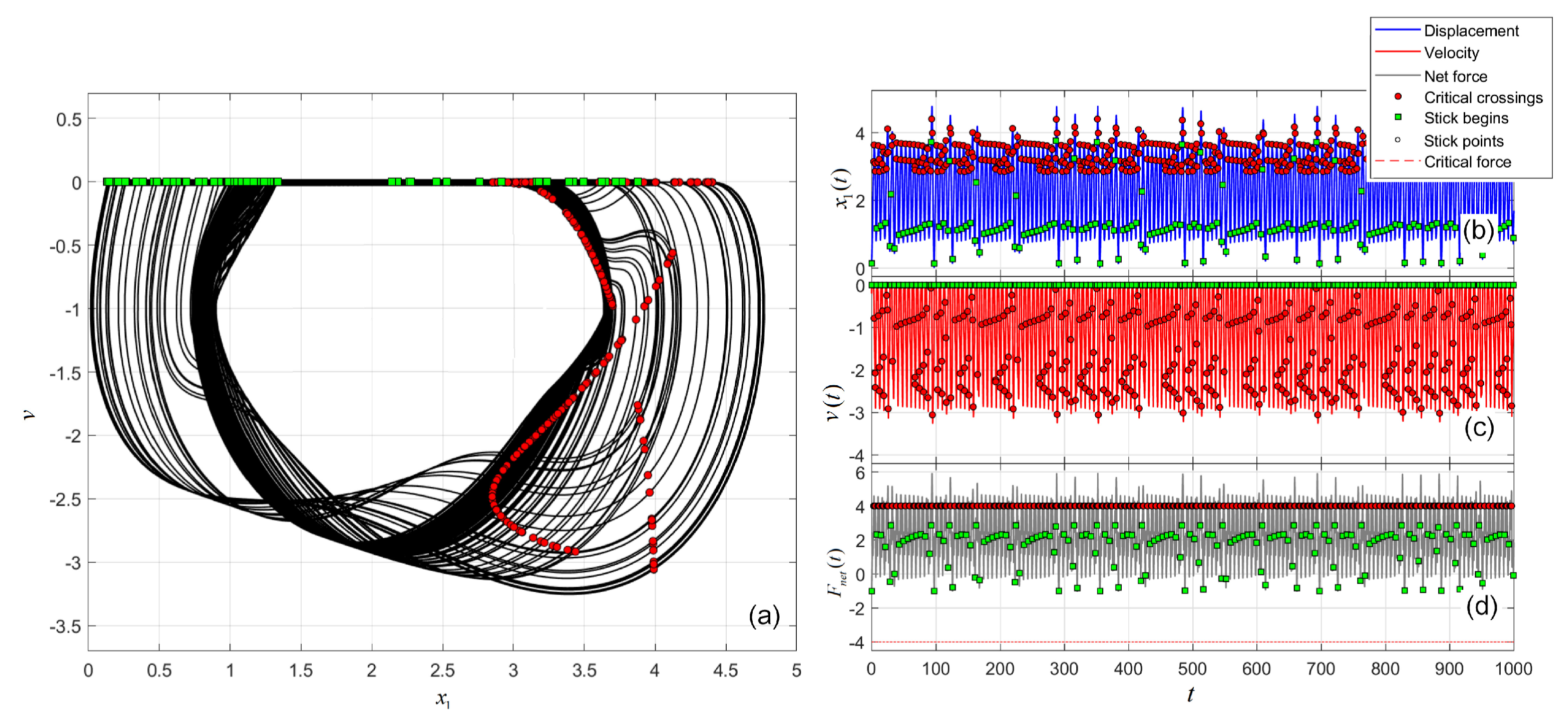
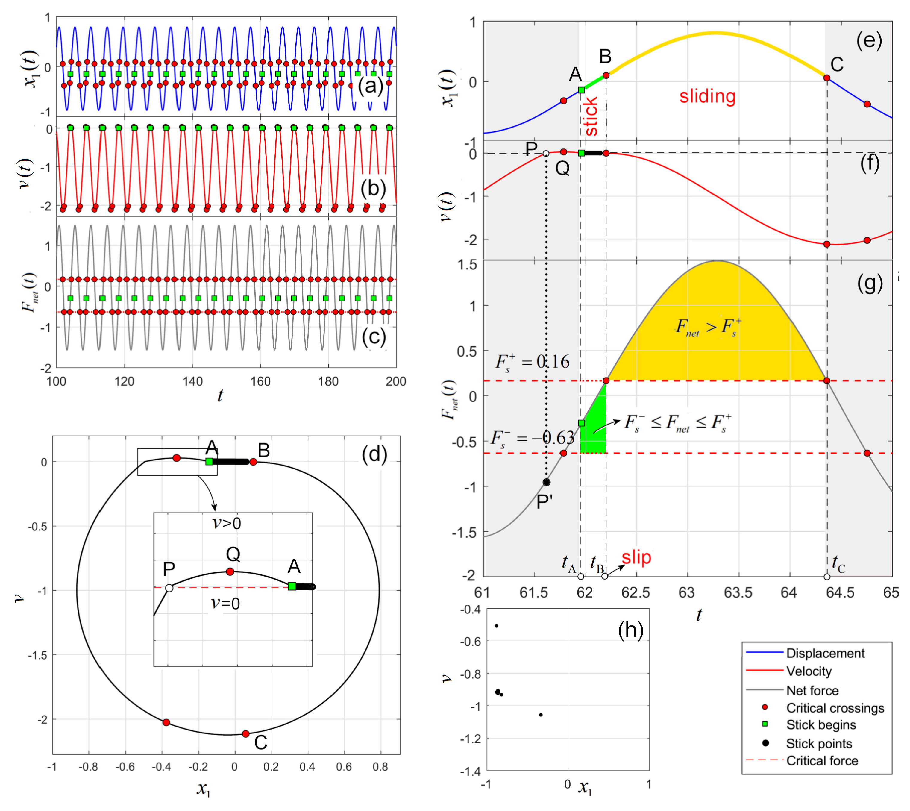
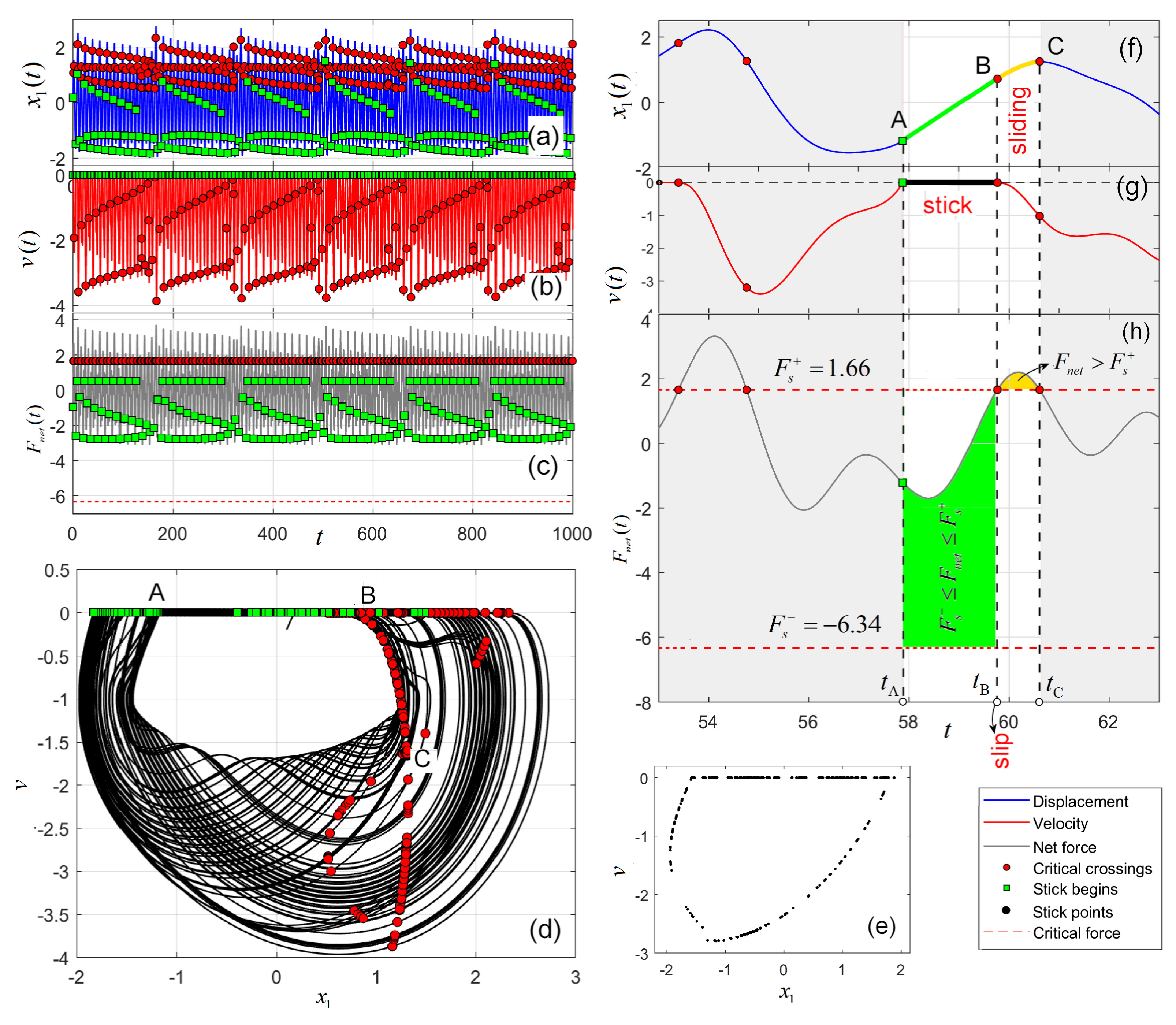
Quasiperiodic Stick–Slip Attractor. Let parameters be $\mathcal{P}$, and $\eta =2.145$, $\gamma =1.15$. The attractor is quasiperiodic stick–slip motion on a 2D Torus in the 3D space $(x_1,v,\varphi )$, a fact revealed by the projections of this torus in the plane $(x_1,v)$ (Figure 7a–d) and the Largest Lyapunov Exponent (LLE), $LLE\approx 0$. The quasiperiodic character is underlined also in the phase plot $(x_1,v)$ in the Poincaré section $\varphi =0 (\mathrm{mod} 2\pi )$ (Figure 7e), where one can see the curve tends to be closed). The two frequencies (one due to stick–slip of the friction dynamics and one due to driving frequency $\eta =2.145$) are irrationally related, causing the trajectory to never exactly repeat but densely cover the torus surface. The critical forces are $F_s^{-}=6.34$ and $F_s^{+}=1.66$ (Figure 7h).

In the zoomed images in Figure 7f–h, the time interval $[t_A,t_C]$ captures the stick–slip phenomenon which starts at $t_A$ (Point A, green rectangle on displacement curve $x_1$). This happens when $F_{\mathrm{net}}$ is within the admissible interval $[F_s^{-},F_s^{+}]$ (green area in the Graph($F_{\mathrm{net}}$)) and v crosses the axis $v=0$. The green arc $\stackrel{⌢}{AB}$ represents the stick displacement. This preslides occurs because real-world contacts are not perfectly rigid but compliant. The moment when the trajectory exits the axis $v=0$ and the stick ends (point B, red circle), due to $F_{\mathrm{net}}$, which overcomes the superior limit $F_s^{+}$ (yellow area in the Graph($F_{\mathrm{net}}$)), represents the slip moment ($t_B$). After $t_B$, for $t\in (t_B,t_C]$, the system is sliding along the yellow arc $\stackrel{⌢}{BC}$, after which the phenomena repeat along the attractor.

Chaotic stick–slip attractor. Let the parameters $\mathcal{P}$ and $\eta =2.848$, $\gamma =1.15$. As Figure 8a–d show, the obtained stick–slip attractor is chaotic.

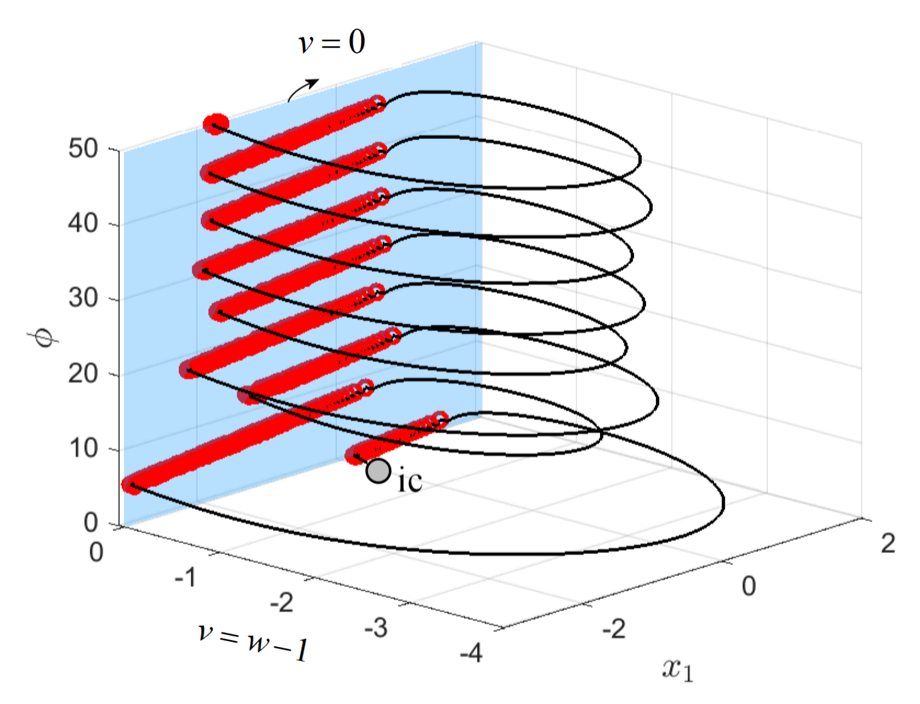
Stable Stick–Slip Cycle Attractor. For parameters $\mathcal{P}$ and $\gamma =0.7,\eta =1.34,a=1$, one obtains the attractor in Figure 6. In this case LLE = −0.002, and the time series in Figure 6a,b together with the Poincare section $\varphi =0 ($mod $2\pi )$ (Figure 6d), show a stable cycle. The stick phase begins at $t_A$, continues for $t\in [t_A,t_B)$ along the arc $\stackrel{⌢}{AB}$, where the system is stick; it slips at $t=t_B$ and is sliding along the attractor on the arc $\stackrel{⌢}{BC}$.

Compared to the other cases, in this case, one can see that v crosses the axis $v=0$ at point P, but the stick does not begin because the condition $F_{\mathrm{net}}\in [F_s^{-},F_s^{+}]$ is not verified and $F_{\mathrm{net}}<F_s^{-}$ (point P’ in Figure 6g). Once $F_{\mathrm{net}}$ hits the critical line, $F_s^{-}$ (critical point Q), v is forced to approach again the line $v=0$, where the stick begins (now $F_{\mathrm{net}}\in [F_s^{-},F_s^{+}]$).

Remark 5. (i)   

If both conditions $v=0$ and $F_{\mathrm{net}}\in [F_s^{-},F_s^{+}]$ are not verified, the stick phase does not appear (red critical points, and in Figure 6, the points P and P’, beside red points).

(ii)     

In all considered cases, the system is perpetually oscillating between the stick and slip states. Although stuck is a fundamental possible state for this system, for the considered parameters, no stuck phase has been found.

5. Fractional Stick–Slip Attractors of the Friction System

To account for the underlying memory effects in the dynamics of the considered friction oscillator, consider a fractional-order formulation based on the Caputo derivative.

Let $q\in (0,1]$, and consider first the IVP of fractional order

$$\left\{\begin{array}{cc}{}^{C}D_{\ast }^{q}x\left(t\right)=f\left(x\left(t\right)\right),\hfill & t\ge 0,\hfill \\ x\left(0\right)=x_0,\hfill \end{array}\right.$$

(16)

where ${}^{C}D_{\ast }^q$ denotes the Caputo derivative of order q with respect the initial moment $t=0$, and f is smooth enough. Caputo’s fractional derivative is defined as follows:

$${}^{C}D_{\ast }^{q}f\left(t\right)={\displaystyle \frac{1}{\mathrm{\Gamma }(1-q)}}{\int }_0^t{\displaystyle \frac{f^{\prime }\left(\tau \right)}{{(t-\tau )}^q}}d\tau ,$$

where $\mathrm{\Gamma }(·)$ is the Gamma function. Unlike the Riemann–Liouville derivative, Caputo’s definition permits the use of conventional (integer-order) initial conditions, which makes it particularly convenient in applied problems and physical modeling. Incorporating this operator into the governing equations of the friction oscillator introduces hereditary effects, reflecting the system’s dependence not only on its instantaneous state but also on its past history.

Consider Caputo’s fractional form of the friction oscillator (5):

$$\begin{array}{cc}\hfill {}^{C}D_{\ast }^{q}x=& v+1,\hfill \\ \hfill {}^{C}D_{\ast }^{q}v=& -x_1-a(\mu \left(1\right)+\mu \left(v\right)sign\left(v\right))+\gamma cos\left(\varphi \right), x\left(0\right)=(x_{10},v_0,{\varphi }_0)\hfill \\ \hfill {}^{C}D_{\ast }^q\varphi =& \eta .\hfill \end{array}$$

(17)

Using the approach in Section 3.1, the IVP (17) can be restarted as the following fractional differential inclusion (FDI):

$$\begin{array}{cc}\hfill {}^{C}D_{\ast }^{q}x=& v+1,\hfill \\ \hfill {}^{C}D_{\ast }^{q}v\in & -x_1-a(\mu \left(1\right)+\mu \left(v\right)Sign\left(v\right))+\gamma cos\left(\varphi \right), x\left(0\right)=x_0, \mathrm{for} \mathrm{a}.\mathrm{e}. t\in I,\hfill \\ \hfill {}^{C}D_{\ast }^q\varphi =& \eta .\hfill \end{array}$$

(18)

Despite FDIs generalizing FDEs to the set-valued case, allowing modeling of non-smooth or uncertain dynamics, they require more advanced tools from set-valued and fractional analysis. Therefore, as for the IO case, the set-valued problem (18) will be transformed into a single-valued problem (see Section 3.2):

$$\begin{array}{cc}\hfill {}^{C}D_{\ast }^{q}x=& v+1,\hfill \\ \hfill {}^{C}D_{\ast }^{q}v=& -x_1-a(\mu \left(1\right)+\mu \left(v\right){sign}_{\epsilon }\left(v\right))+\gamma cos\left(\varphi \right), x\left(0\right)=x_0,\hfill \\ \hfill {}^{C}D_{\ast }^q\varphi =& \eta .\hfill \end{array}$$

(19)

The existence and uniqueness of solutions to the general IVP (16) are ensured similarly to Theorem 4 (see also [30])

Theorem 5. 

The fractional IVP (19) admits a unique solution.

Proof. 

As known FDEs admit unique solutions if the RHS is locally or globally Lipschitz continuous, Theorem 4 applies (see also [31]). □

The system has memory, and now, due to the fractional derivative, the phase $\varphi$ itself evolves with a temporal history dependency. Because for low fractional order q, the present behavior is significantly influenced by very old state values, and the computational time is higher, q is chosen as $q=0.9$ when only relatively recent history matters.

The numerical implementation requires storing the entire history and using efficient memory management techniques such as the Adams–Bashforth–Moulton numerical scheme for FDEs, utilized here [30], with the integration step size $h=0.001$. To simulate the fractional stick–slip attractors, the algorithm used to obtain the integer order system is used, but with the MATLAB solver ode45 replaced with the ABM predictor–corrector numerical scheme.

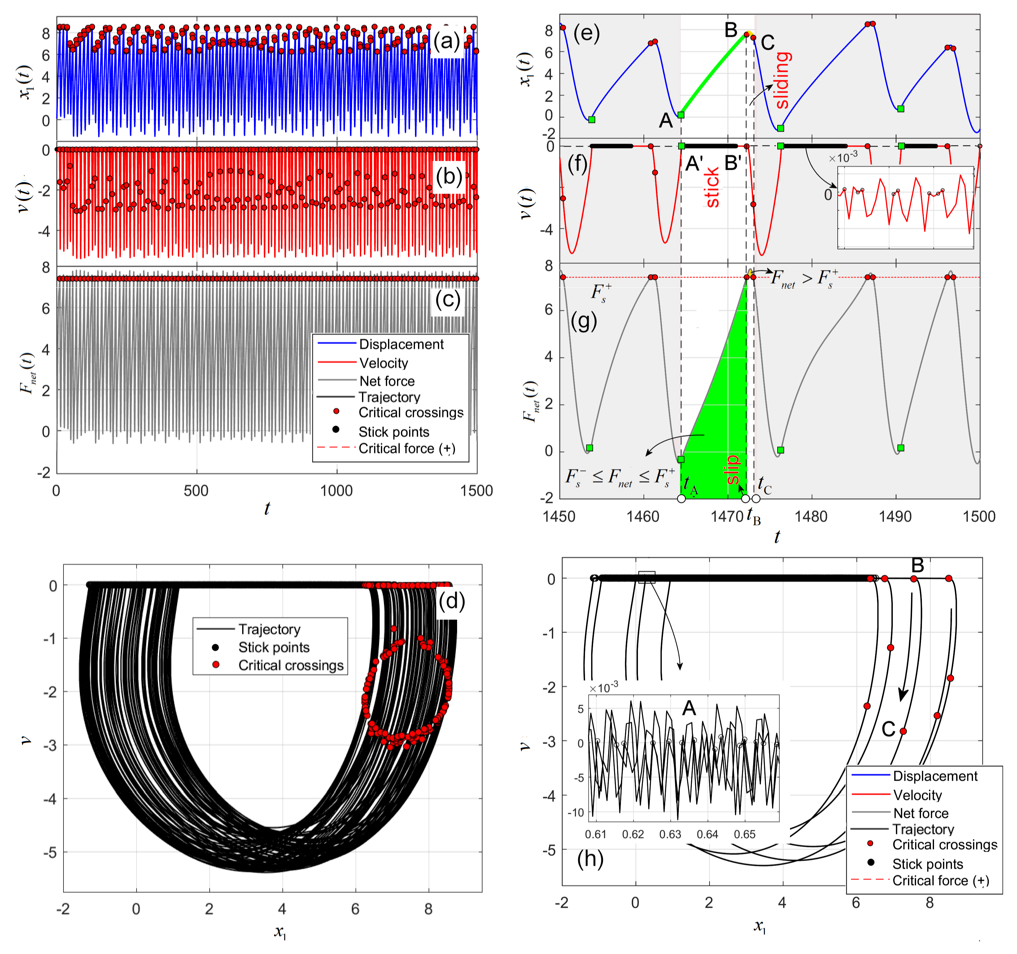
Fractional chaotic stick–slip attractor. Consider the parameters ${\mu }_0=2,{\mu }_1=0.1,{\lambda }_0=1.42, {\lambda }_1=0.02, \gamma =1.15, \eta = 1.45, a =2.15$. The attractor is chaotic with LLE = 18.89, obtained with the MATLAB code presented in [32] (see also [33]). The results are presented in Figure 9. The time series and the phase plot indicate the chaotic stick–slip motion.

As known, compared to the schemes for ODEs (like the used ode45 solver), where the adaptive step size is straightforward, the integration of FDEs choosing the step size is difficult, not to mentioning the computational cost ($O\left(N\right)$ for ode45 vs $O\left(N^2\right)$ (N steps $\times N$ history) for ABM, or local truncation error $O\left(h^5\right)$ and global error $O\left(h^4\right)$ for ode45 vs the accuracy $O\left(h^p\right)$ where $p=min\{2,1+q\}$). Therefore, finding the fractional stick–slip phenomenon represented a challenge (see, for example, the zoom in Figure 9b and the phase plot in Figure 9h, where the first transients have been discarded).

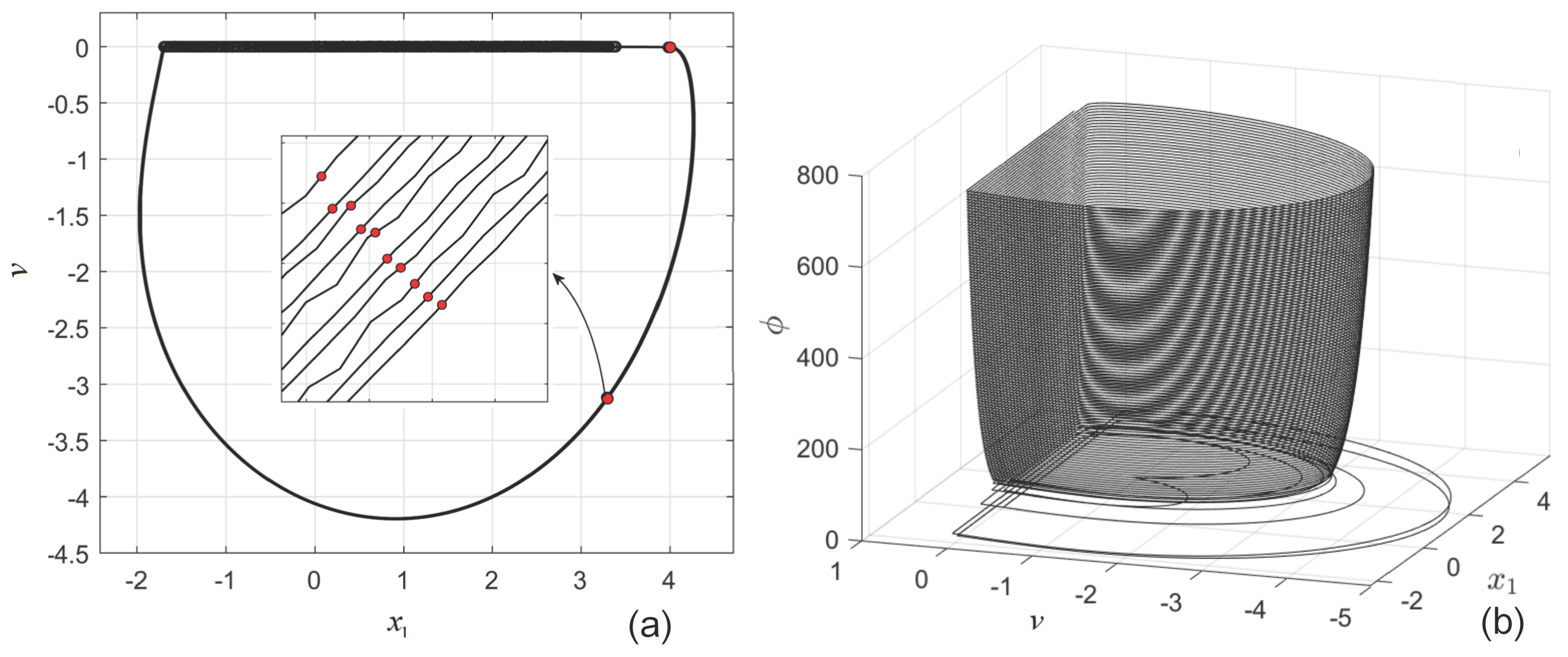
Fractional “apparent periodic” stick–slip attractor. The most interesting and striking behavior is observed for the parameter set ${\mu }_0=2$, ${\mu }_1=0.1$, ${\lambda }_0=1.42$, ${\lambda }_1=0.02$, $\gamma =1.15$, $\eta =0.7$, and $a=10$, as shown in Figure 10. Although the phase plot (Figure 10a) and the trajectory in the space $(x_1,v,\varphi )$ appear to suggest a stable, periodic stick–slip motion, the actual behavior is fundamentally different. It is well known that fractional differential equations (FDEs) formulated with Caputo derivatives (as well as with Riemann–Liouville or Gr“unwald–Letnikov derivatives) cannot possess non-constant periodic solutions [34], a property stemming from their nonlocal nature and the long-range dependence on the entire history of the system.

Therefore, even when trajectories appear periodic, the system—like all autonomous fractional systems defined with these derivatives—cannot exhibit true periodic behavior. A zoomed-in view in Figure 10a reveals that the trajectory is not precisely closed, even within reasonably small numerical errors. This deviation is not solely due to numerical inaccuracies but also reflects the intrinsic non-periodicity of FDEs. In conclusion, the system evolves according to stick–slip dynamics, but now in an “apparently periodic” manner.

6. Hidden Chaotic Attractors

Definition 3. 

An attractor is called hidden if its basin of attraction does not intersect with any small neighborhood of an equilibrium point of the system. Conversely, an attractor is called self-excited if its basin of attraction is associated with an unstable equilibrium.

Proposition 3. 

All attractors of the IO or FO systems (5), or (17), respectively, are hidden attractors.

Proof. 

The systems do not have equilibria, and Definition 3 applies. □

The risk associated with a hidden attractor depends heavily on the system’s equilibria. Thus, for example, in systems with stable equilibria, a hidden attractor represents a critical “trapdoor”: the system appears locally stable, giving a “false sense of security”, but a disturbance (less or more large) can push it irreversibly into a dangerous, oscillatory state, compared to systems without equilibria, where all (hidden) attractors can be easily found and where that risk theoretically does not exist.

7. Conclusions

This paper investigates stick–slip attractors in a friction oscillator of IO and FO order. Due to the non-existence of the solutions of the underlying IVP, it is proved analytically how the discontinuous IVP can be approximated with a continuous problem. For this purpose, Filippov’s regularization is used, and the discontinuous problem is restarted as a DI. Next, using Cellina’s selection theorem, the set-valued problem transforms into a single-valued continuous one, which can be numerically approached by using standard schemes for DEs or FDEs. The simulations show that the system admits quasiperiodic stick–slip attractors, chaotic stick–slip attractors, and stable stick–slip cycle attractors. The special cases of the FO stick–slip attractors are carefully analyzed, and the non-existence of periodic oscillations is analyzed numerically.

References

1. Heslot, F.; Baumberger, T.; Perrin, B.; Caroli, B.; Caroli, C. Creep, stick-slip, and dry-friction dynamics: Experiments and a heuristic model. Phys. Rev. E 1994, 49, 12184–12189. [Google Scholar] [CrossRef] [PubMed]
2. Rabinowicz, E. Friction and Wear of Materials, 2nd ed.; Wiley: Hoboken, NJ, USA, 1995. [Google Scholar]
3. Popov, V.L. Contact Mechanics and Friction; Springer: Berlin, Germany, 2010. [Google Scholar]
4. Wiercigroch, M.; de Kraker, B. Applied Nonlinear Dynamics and Chaos of Mechanical Systems with Discontinuities; World Scientific Series on Nonlinear Science, Series A (Vol. 28); World Scientific: Singapore, 2000. [Google Scholar]
5. Baumberger, T.; Caroli, C. Solid friction from stickñslip down to pinning and aging. Adv. Phys. 2006, 55, 279–348. [Google Scholar] [CrossRef]
6. Persson, B.N.J. Sliding Friction: Physical Principles and Applications; Springer: Berlin, Germany, 2000. [Google Scholar]
7. di Bernardo, M.; Budd, C.J.; Champneys, A.R.; Kowalczyk, P. Piecewise-Smooth Dynamical Systems: Theory and Applications; Springer: Berlin, Germany, 2008. [Google Scholar]
8. Brogliato, B. Nonsmooth Mechanics: Models, Dynamics, and Control, 3rd ed.; Springer: Berlin, Germany, 2016. [Google Scholar]
9. Filippov, A.F. Differential Equations with Discontinuous Righthand Sides; Kluwer Academic Publishers: Alphen aan den Rijn, The Netherlands, 1988. [Google Scholar]
10. Leine, R.I.; Nijmeijer, H. Dynamics and Bifurcations of Non-Smooth Mechanical Systems; Springer: Berlin, Germany, 2004. [Google Scholar]
11. Popp, K.; Hinrichs, N.; Oestreich, M. Dynamical behaviour of friction oscillators with stickñslip motion. Philos. Trans. R. Soc. 1999, 357, 3119–3136. [Google Scholar]
12. Liberzon, D. Switching in Systems and Control; Birkhauser: Basel, Switzerland, 2012. [Google Scholar]
13. Utkin, V.I. Sliding Modes in Control and Optimization; Springer: Berlin, Germany, 1992. [Google Scholar]
14. Jeffrey, M.R. Non-Smooth Dynamics; Springer: Berlin, Germany, 2018. [Google Scholar]
15. di Bernardo, M.; Vasca, F. Discontinuities in interconnected systems: A survey. Annu. Rev. Control 2010, 34, 1–17. [Google Scholar]
16. Podlubny, I. Fractional Differential Equations; Academic Press: Cambridge, MA, USA, 1999. [Google Scholar]
17. Kilbas, A.A.; Srivastava, H.M.; Trujillo, J.J. Theory and Applications of Fractional Differential Equations; Elsevier: Amsterdam, The Netherlands, 2006. [Google Scholar]
18. Mainardi, F. Fractional Calculus and Waves in Linear Viscoelasticity; Imperial College Press: London, UK, 2010. [Google Scholar]
19. Metzler, R.; Klafter, J. The random walk’s guide to anomalous diffusion: A fractional dynamics approach. Phys. Rep. 2000, 339, 1–77. [Google Scholar] [CrossRef]
20. Petráš, I. Fractional-Order Nonlinear Systems: Modeling, Analysis and Simulation; Springer: Berlin, Germany, 2011. [Google Scholar]
21. Magin, R.L. Fractional Calculus in Bioengineering; Begell House: Danbury, CT, USA, 2006. [Google Scholar]
22. Dudkowski, J.; Jafari, S.; Capitaine, T.; Kuznetsov, N.V.; Leonov, G.A.; Prasad, A. Hidden attractors in dynamical systems. Phys. Rep. 2016, 637, 1–50. [Google Scholar] [CrossRef]
23. Kunze, M.; Küpper, T. Qualitative bifurcation analysis of a non-smooth friction-oscillator model. Z. Angew Math. Phys. 1997, 48, 87–101. [Google Scholar] [CrossRef]
24. Danca, M.-F. Solutions of a Class of Switch Dynamical Systems. Entropy 2025, 27, 158. [Google Scholar] [CrossRef] [PubMed]
25. Danca, M.-F.; Fečkan, M. On Numerical Integration of Discontinuous Dynamical Systems. Int. J. Bifurc. Chaos 2017, 27, 1750218. [Google Scholar] [CrossRef]
26. Aubin, J.-P.; Cellina, A. Differential Inclusions: Set-Valued Maps and Viability Theory; Springer: Heidelberg, Germany, 1984. [Google Scholar]
27. Aubin, J.-P.; Frankowska, H. Set-Valued Analysis; Birkhauser: Basel, Switzerland, 1990. [Google Scholar]
28. Kastner-Maresch, A.; Lempio, F. Difference methods with selection strategies for differential inclusions. Numer. Funct. Anal. Optim. 1993, 14, 555–572. [Google Scholar] [CrossRef]
29. Taubert, K. Converging Multistep Methods for Initial Values Problems Involving Multivalued Maps. Computing 1981, 27, 123–136. [Google Scholar] [CrossRef]
30. Diethelm, K.; Ford, N.J. Analysis of fractional differential equations. J. Math. Anal. Appl. 2002, 265, 229–248. [Google Scholar] [CrossRef]
31. Diethelm, K. The Analysis of Fractional Differential Equations; Springer: Berlin, Germany, 2010. [Google Scholar]
32. Danca, M.-F.; Kuznetsov, N. Matlab code for Lyapunov exponents of fractional order systems. Int. J. Bifurc. Chaos 2018, 28, 1850067. [Google Scholar] [CrossRef]
33. Danca, M.-F.; Feckan, M. Memory Principle of the MATLAB Code for Lyapunov Exponents of Fractional-Order. Int. J. Bifurc. Chaos 2024, 2450156. [Google Scholar] [CrossRef]
34. Tavazoei, M.S.; Haeri, M. A proof for non existence of periodic solutions in time invariant fractional order systems. Automatica 2009, 45, 1886–1890. [Google Scholar] [CrossRef]
Figure 1. (a) The friction oscillator; (b) The nonlinear friction force a [ μ ( 1 ) + μ ( x ˙ 1 ) sign ( x ˙ 1 ) ] .
Fractalfract 10 00038 g001
Figure 2. (a) Solutions of the problem (7), with x 0 0 , cannot continue on the axis x = 0 ; (b) After regularization, the solutions of the problem (7) can be defined along the axis x = 0 ; (c) The graph of the set-valued Sign function [25].
Fractalfract 10 00038 g002
Figure 3. (a) Sketch of the Approximation Theorem 2; (b) Sketch for local approximations within a small neighborhood of discontinuity; (c) Graph of the discontinuous function H (14); (d) Graph of the regularized function H; (e) Graph of the approximated function (for a relative larger δ in (12)).
Fractalfract 10 00038 g003
Figure 4. Chart of the continuous approximation of the IVP (5).
Fractalfract 10 00038 g004
Figure 5. A solution to the IVP (5).
Fractalfract 10 00038 g005
Figure 6. Stable stick–slip cycle attractor for parameters P and γ = 0.7 , η = 1.34 and a = 1 ; (ac) Time series for x 1 , v, and F net , respectively; (d) Phase plot; (eg) Zoomed details showing the stick–slip states; (h) Poincaré section ϕ = 0   ( mod 2 π ) . The critical point P does not start the stick phenomenon (see point P’).
Fractalfract 10 00038 g006
Figure 7. Quasiperiodic stick–slip attractor corresponding to parameters P and γ = 1.15 , η = 2.145 , and a = 10 ; (ac) Time series for x 1 , v and F net , respectively; (d) Phase plot; (e) Poincaré section ϕ = 0 ( mod   2 π ). Points A, B and C (d,f) and t a , t B , and t C indicate the stick–slip and sliding states; (fh) Zoomed time series indicating the stick phase, slip moment, and sliding phase.
Fractalfract 10 00038 g007
Figure 8. Chaotic stick–slip attractor for parameters P and γ = 1.15 , η = 2.848 and a = 10 ; (a) Phase plot; (bd) Time series of x 1 , v, and F net , respectively.
Fractalfract 10 00038 g008
Figure 9. Chaotic fractional stick–slip attractor for parameters μ 0 = 2 , μ 1 = 0.1 , λ 0 = 1.42 , λ 1 = 0.02 , γ = 1.15 , e t a = 1.45 , and a = 2.15 ; (ac) Time series of x 1 , v and F net , respectively; (d) Phase plot; (eg) Zoomed time series indicating the stick–slip phases; (h) Phase plot obtained for short time integration interval to unveil the attractor dynamics: Zoomed details in Figure 9f,h show the errors inherent to numerical integration of FDEs. Also, the stick moments (like the segment A’B’) cannot be exactly determined for the same reasons.
Fractalfract 10 00038 g009
Figure 10. “Apparent-Periodic” fractional stick–slip attractor for parameters μ 0 = 2 , μ 1 = 0.1 , λ 0 = 1.42 , λ 1 = 0.02 , γ = 1.15 , η = 1.45 , a = 2.15 ; (a) Phase plot; (b) 3D representation of the attractor. Although the 3D phase plot would indicate a “periodic” motion, the zoomed detail in Figure 10a, together with the result of non-existence of periodicity in FO systems underline the fact that this attractor is not periodic.
Fractalfract 10 00038 g010
Disclaimer/Publisher’s Note: The statements, opinions and data contained in all publications are solely those of the individual author(s) and contributor(s) and not of MDPI and/or the editor(s). MDPI and/or the editor(s) disclaim responsibility for any injury to people or property resulting from any ideas, methods, instructions or products referred to in the content.