Article

Online Asynchronous Learning over Streaming Nominal Data

1
Jinan University & University of Birmingham Joint Institution, Jinan University, Guangzhou 510632, China
2
College of Cyber Security, Jinan University, Guangzhou 510632, China
3
School of Intelligent Science and Technology, Beijing University of Civil Engineering and Architecture, Beijing 100044, China
*
Author to whom correspondence should be addressed.
Big Data Cogn. Comput. 2025, 9(7), 177; https://doi.org/10.3390/bdcc9070177
Submission received: 2 June 2025 / Revised: 29 June 2025 / Accepted: 30 June 2025 / Published: 2 July 2025

Abstract

Online learning has become increasingly prevalent in real-world applications, where data streams often comprise heterogeneous feature types—both nominal and numerical—and labels may not arrive synchronously with features. However, most existing online learning methods assume homogeneous data types and synchronous arrival of features and labels. In practice, data streams are typically heterogeneous and exhibit asynchronous label feedback, making these methods insufficient. To address these challenges, we propose a novel algorithm, termed Online Asynchronous Learning over Streaming Nominal Data (OALN), which maps heterogeneous data into a continuous latent space and leverages a model pool alongside a hint mechanism to effectively manage asynchronous labels. Specifically, OALN is grounded in three core principles: (1) It utilizes a Gaussian mixture copula in the latent space to preserve class structure and numerical relationships, thereby addressing the encoding and relational learning challenges posed by mixed feature types. (2) It performs adaptive imputation through conditional covariance matrices to seamlessly handle random missing values and feature drift, while incrementally updating copula parameters to accommodate dynamic changes in the feature space. (3) It incorporates a model pool and hint mechanism to efficiently process asynchronous label feedback. We evaluate OALN on twelve real-world datasets; the average cumulative error rates are 23.31% and 28.28% under the missing rates of 10% and 50%, respectively, and the average AUC scores are 0.7895 and 0.7433, which are the best results among the compared algorithms. And both theoretical analyses and extensive empirical studies confirm the effectiveness of the proposed method.

1. Introduction

Online learning [1,2,3,4,5] has achieved significant success in recent years across a wide range of domains, particularly in scenarios involving continuously arriving data streams. Unlike traditional batch learning methods, which require access to the entire dataset upfront, online learning incrementally updates models in real time as new data become available [6]. This characteristic substantially reduces computational and storage overheads, while providing notable adaptability to complex real-world applications, such as natural disaster monitoring in ecological systems [7], real-time credit card fraud detection [8], and skin disease diagnosis [9,10]. As a result, online learning has emerged as a pivotal technique for data stream analytics in the era of big data.
Existing online learning techniques are generally categorized into two paradigms: online static learning [11] and online dynamic learning [12]. Online static methods, having been developed earlier, have accumulated a substantial body of research and are valued for their simplicity, computational efficiency, and ease of deployment. By leveraging incremental gradient updates and regularization, these approaches effectively handle stable data distributions, particularly in resource-constrained environments [11]. In contrast, online dynamic learning emphasizes adaptability to non-stationary data distributions and evolving feature spaces [13]. Through feature mapping and embedding strategies, these methods dynamically adjust model parameters, thereby maintaining high predictive performance even as feature dimensions or data sources grow increasingly complex [14]. Furthermore, real-world data streams often contain mixed-type variables [15,16], introducing additional challenges to the learning process.
Nevertheless, despite their individual strengths, existing methods face significant limitations in complex real-world environments, particularly in addressing two key challenges. First, the dynamic evolution of mixed feature spaces—comprising both numerical and nominal attributes—often leads to changes in feature dimensionality [17,18], making it difficult for traditional methods to maintain predictive performance. Second, the asynchronous nature of data streams, in which features and labels arrive at irregular intervals and from diverse sources, frequently results in incomplete or delayed information that adversely affects model training [19,20,21]. Accordingly, the development of an effective online learning algorithm capable of simultaneously managing mixed-type data, evolving feature spaces, and asynchronous arrivals of features and labels has become a critical and urgent research challenge—one that motivates the primary objective of this study.
Our proposed method, Online Asynchronous Learning over Streaming Nominal Data (OALN), presents a unified framework designed to address missing data and asynchronous supervision in dynamic data streams through the integration of three key components. First, it incorporates a real-time imputation module that combines a Gaussian Copula model with an online expectation-maximization algorithm to jointly estimate feature distributions and impute missing values for both nominal and numerical attributes, thereby ensuring statistical consistency and completeness across heterogeneous feature spaces. Second, to maintain predictive robustness under evolving data characteristics, OALN trains multiple classifiers on the imputed feature space and integrates their predictions using adaptively updated ensemble weights. Third, it introduces a simulated delay mechanism to model the asynchronous arrival of features and labels, substantially enhancing the model’s resilience in real-world scenarios characterized by irregular and non-synchronized inputs. An overview of the proposed framework is presented in Figure 1.
To achieve the aforementioned advantages, this paper makes the following key contributions:
(1)
We formally identify and unify the challenges of evolving feature spaces, heterogeneous data types, and asynchronous label arrivals within a coherent online learning framework.
(2)
We propose a novel algorithm, termed OALN, which integrates real-time estimation of mixed-type feature distributions via an Extended Gaussian Copula model, coupled with an adaptive and incremental learning strategy tailored to dynamic and asynchronous data streams.
(3)
We design a comprehensive evaluation framework that jointly simulates evolving feature dimensions, mixed-type data, and asynchronous label availability, thereby enabling a rigorous assessment of OALN ’s robustness and practical applicability.
The remainder of this paper is organized as follows: Section 2 reviews the related work. Section 4 introduces the construction of the latent feature space and the handling of asynchronous labels to capture feature preferences. Section 5 presents the experimental results and discussions. Finally, Section 6 concludes the paper and outlines directions for future research.

2. Related Work

This work is related to online static learning [11], online dynamic learning [12], and asynchronous learning methods [19,22,23]. As shown in Table 1, although extensive research has been conducted in the field of online learning [24,25,26,27], few studies have addressed scenarios involving incomplete feature spaces and the asynchronous arrival of mixed-type data streams. In real-world applications, data streams often arrive asynchronously with varying delays [21,28], leading to incomplete and dynamically evolving feature spaces, where conventional online learning methods demonstrate limited effectiveness. To tackle these challenges, this study introduces a novel online learning framework, termed OALN, which integrates the incremental updating capability of online static learning, the adaptability of online dynamic learning for continuously evolving feature spaces, and the robustness of asynchronous learning methods for handling irregularly arriving data. The subsequent sections will provide a comprehensive review of existing studies on online static learning, online learning in dynamic feature spaces, and asynchronous learning methods, highlighting their limitations in practical scenarios.

2.1. Online Static Learning

Online static learning is one of the earliest and most extensively studied paradigms in the field of online learning [11]. It assumes that data arrive sequentially over time while the underlying distribution remains relatively stable. Based on this assumption, existing methods employ incremental gradient updates and regularization techniques, allowing efficient updates to model parameters upon receiving each new data instance, with minimal computational overhead. For example, in scenarios such as embedded systems or real-time analytics platforms, online static learning algorithms are well-suited for delivering low-latency predictions and high throughput due to their inherently incremental nature.
Nonetheless, these methods assume that the data distribution remains unchanged and that the feature space is fixed and complete—conditions that are often violated in real-world settings [24,32]. In practice, data may arrive with irregular delays [28,33,34], exhibit random feature omissions, or involve dynamically evolving feature spaces with mixed data types [35]. Under such circumstances, traditional online static learning models struggle to adapt, leading to significant declines in predictive performance. Consequently, these limitations hinder their ability to meet the stringent requirements for stability and accuracy in complex real-world scenarios. However, our OALN algorithm integrates mixed-feature modeling and real-time imputation with incremental updates, thereby ensuring stable predictive accuracy even in incomplete or evolving feature spaces.

2.2. Online Learning in Dynamic Feature Space

Online learning in dynamic feature spaces focuses on adapting models to feature sets that expand or contract as new data arrive [36]. Such methods typically employ mapping or embedding strategies to reconcile discrepancies between old and new feature dimensions, allowing the learned parameters to be shared or transferred [37]. Some approaches use linear transformations to align features, while others adopt nonlinear or kernel-based strategies to handle complex mappings more effectively [12,14]. By dynamically adjusting model parameters as the feature space evolves [15], these methods aim to maintain strong predictive accuracy despite shifting or expanding feature sets.
Although current approaches to dynamic feature space learning better accommodate the variability in incoming data, they often focus primarily on numerical features or assume a relatively stable marginal distribution [38]. When applied to more heterogeneous contexts (e.g., nominal features or missing data), these methods may fail to preserve critical structural information that cannot be captured by linear or simplified mappings [20,28]. Moreover, balancing model complexity with adaptation frequency remains a challenge: overly frequent model updates can incur high computational costs, while infrequent updates may result in degraded accuracy as the feature space evolves. Nevertheless, our OALN algorithm leverages real-time estimation of mixed-feature distributions and adaptive incremental updates, enabling efficient and accurate learning even under frequent changes in feature dimensionality.

2.3. Asynchronous Learning Methods

Asynchronous learning methods are designed to handle data streams that arrive at irregular intervals or with unpredictable delays, allowing the model to update independently of a fixed scheduling mechanism [22,39]. These methods often adopt decentralized or distributed architectures, in which partial updates are accumulated and subsequently integrated into a global model once the data becomes available [40,41]. By decoupling training from a synchronized data arrival schedule, asynchronous approaches offer robustness against real-world contingencies such as network latencies, sensor malfunctions, or uneven data rates [19,42].
Despite their robustness to timing irregularities, many asynchronous learning methods still assume a relatively complete and stable feature set and expect labels to be available in tandem with the data [43,44]. In practice, delayed or missing labels, along with mixed data types such as nominal and numerical features, can significantly degrade the performance of these methods [31,39,45]. Moreover, coordination overhead may become a bottleneck in large-scale scenarios, where numerous asynchronous model updates must be merged without losing critical information or introducing inconsistencies [40]. In contrast, our OALN algorithm integrates asynchronous updates with mixed-feature adaptive modeling, allowing the model to learn from partial data without requiring full synchronization, while maintaining predictive robustness under unpredictable conditions.

3. Problem Statement

The main emphasis of our OALN algorithm lies in binary classification, with the option of straightforward expansion to multiclass scenarios employing One-vs-Rest [46] or One-vs-One [47] strategies. Define an input sequence ( x t , y t ) | t = 1 , 2 , , T as instances arriving in real time, where x t = x 1 , x 2 , , x d t T denotes a vector of dimension d t recorded in instance x t , accompanied by a corresponding label y t { 1 , + 1 } . Moreover, due to practical constraints in data collection and feedback, the label y t corresponding to x t may not be revealed until time t + k , where k 0 . For mixed-type streaming data types, we define x t as ( x nom , x num ) , where x nom and x num represent nominal and numerical variables, respectively. At each round t, the combination of the online learner g ( · , · ) and the current weights β of the model makes a prediction based on the currently available features. Once the label arrives at time t + k , the loss σ ( y t + k , g ( ω i , x t ) ) is computed, and the model is updated accordingly. Our objective is to identify a sequence of functions { g } t = 1 T that can effectively handle both the evolving feature space and the asynchronous arrival of labels. Formally, we define our empirical risk minimization (ERM) objective as:
min R ( T ) = 1 T t = 1 T σ ( y t + k , g ( ω i , x t ) ) , s . t . x t = ( x nom , x num ) ,
where σ ( · , · ) denotes the loss function, measuring the discrepancy between the predicted output and the ground-truth label. y t + k is the true label corresponding to x t , which is collected at time step t + k , and x t is the corresponding input feature vector. By continually updating the online learner, this framework aims to accommodate the dynamic feature space and asynchronous feedback in data streams, ultimately improving predictive performance on evolving data sequences.

4. The Proposed Approach

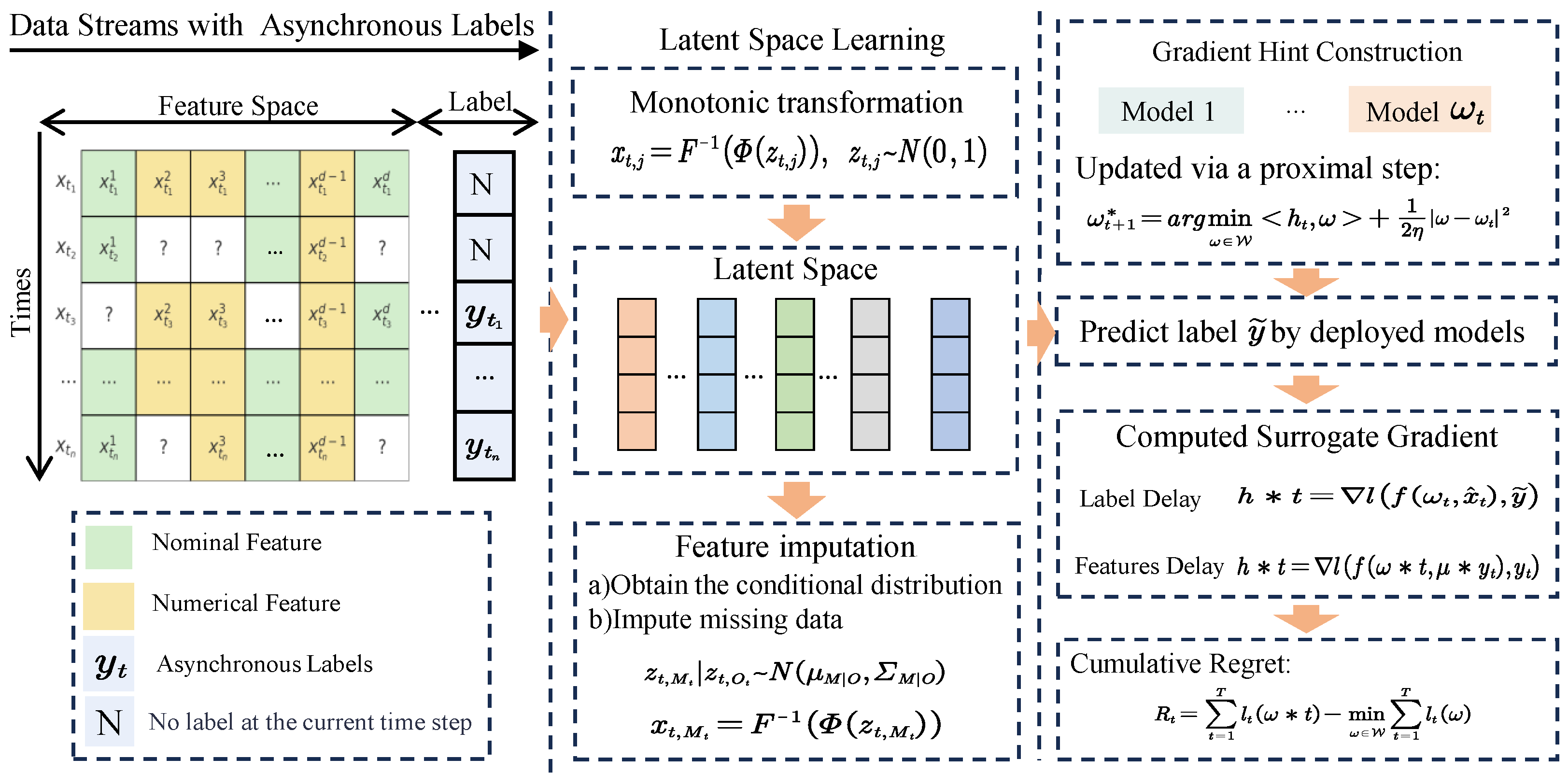
To effectively address the challenges posed by mixed-type, incomplete input features and delayed label feedback in online learning, our approach is composed of two key modules. First, we propose a latent feature encoding and imputation mechanism (Section 4.1) based on the Extended Gaussian Copula, which transforms partially observed, heterogeneous inputs into complete and statistically consistent representations. Second, we design an online learning algorithm (Section 4.2) tailored for asynchronous labels, which utilizes hint-based updates to adaptively learn even when full supervision is not immediately available. Together, these components ensure robustness under both input uncertainty and delayed feedback.

4.1. Latent Feature Encoding and Imputation

In real-time machine learning systems, data often arrives through streaming and in an incomplete manner. Such data typically contains mixed-type features, encompassing nominal (categorical), ordinal, and continuous variables [17,30]. Compounding this challenge is the fact that data collection in practice is imperfect, frequently leading to missing entries due to latency, hardware failure, user interruption, or privacy-preserving protocols. These missing values can occur in both structured input x t R d and the associated labels y t .
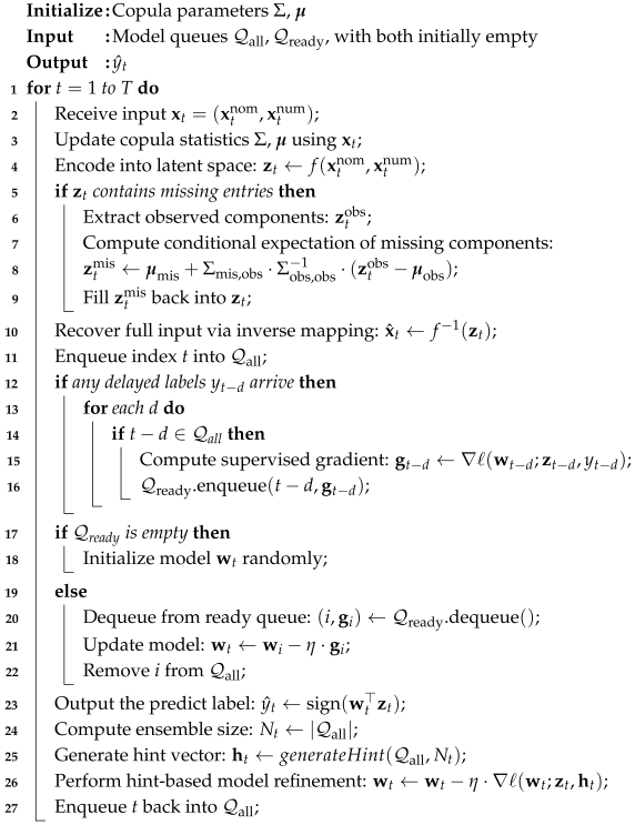
Our learning objective for OALN is to train an online model that maps a sequence of input instances x t = ( x nom , t , x num , t ) to predictions, even when such instances are incomplete or partially observed. To support accurate and robust model training, we must therefore construct a feature representation module that can handle heterogeneous feature types; missing values in arbitrary dimensions; and statistical dependencies across features.
To address this need, we propose a probabilistic latent encoding framework based on the Extended Gaussian Copula (EGC) model, which serves as a front-end encoder for the online learner. We select the Extended Gaussian Copula owing to its formal separation of marginal distributions from the underlying dependence structure, its closed-form and bijective CDF transformations that guarantee statistically coherent and semantically consistent imputations, and its robust covariance estimation amenable to low-rank or diagonal approximations—substantially reducing storage and computational overhead in high-dimensional settings. These attributes collectively provide a theoretically sound and practically efficient encoding mechanism for online learning. This module takes partially observed mixed-type feature vectors as input and outputs fully specified, semantically consistent, and distribution-aware representations x ^ t , which can be safely used in any downstream predictive task.
  • Latent Mapping of Mixed-Type Features. To enable unified modeling of heterogeneous input data x t = ( x t , 1 , x t , 2 , , x t , d ) , which may consist of categorical, ordinal, and continuous variables, we adopt a latent variable framework wherein each observed feature is represented as a transformation of a latent Gaussian variable. The core assumption is that there exists a latent vector z t N ( 0 , Σ ) , from which the observed values are generated via a decoding function f i specific to the type of each variable.
For categorical features x t , i { 1 , , K i } , we define a latent sub-vector z t , i R K i and apply the Gaussian-max transformation:
x t , i = arg max k ( z t , i ( k ) + μ i ( k ) ) , z t , i N ( 0 , I ) ,
where μ i R K i is a learnable shift vector. This operation retains the unordered nature of nominal variables without imposing an artificial structure, while also allowing the modeling of arbitrary categorical distributions through the learned biases μ i .
For ordinal or continuous features x t , j , we adopt a monotonic transformation based on the Gaussian Copula [48]:
x t , j = F j 1 ( Φ ( z t , j ) ) , z t , j N ( 0 , 1 ) ,
where F j is the empirical cumulative distribution function of the observed data and Φ is the standard normal CDF [49]. In an offline setting, F j can be obtained by sorting the full dataset and directly accumulating quantiles; however, in an online streaming environment where it is infeasible to retain all historical samples, one typically discretizes the variable’s domain into bins and maintains the count per bin along with the total sample count. Upon arrival of each new sample, only the corresponding bin count and the overall count are incrementally updated, and the empirical CDF at any value is estimated by dividing the cumulative bin counts below that value by the current total. This scheme supports constant- or logarithmic-time updates, satisfying the real-time requirements of high-throughput data streams while approximately preserving the original marginal distribution. The transformation thus embeds data into a latent Gaussian space without altering its marginal properties.
By applying these transformations across all variables, we obtain a full latent representation z t R D , where D is the sum of the dimensions required for each variable’s encoding. This provides a consistent and information-rich representation of the instance, regardless of missing values.
  • Joint Latent Modeling and Dependency Structure. After constructing the latent representation for all input variables, we assume the complete latent vector follows a multivariate Gaussian distribution:
    z t N ( 0 , Σ ) ,
    where Σ R D × D captures all pairwise dependencies among the latent sub-components. This joint distribution enables the model to learn global correlations between variables of different types, including cross-type dependencies such as correlations between categorical and continuous variables.
Unlike heuristic encoding methods that treat features independently or separately model each type, the EGC framework leverages the joint covariance structure Σ to support statistical coupling between all dimensions. This is particularly important in the presence of missing data, as the unobserved variables can be inferred based on their conditional relationship to the observed ones. Furthermore, the use of empirical marginals in the decoding process ensures that the generated values maintain fidelity to the original data distribution, even when imputed.
This formulation bridges the gap between traditional multivariate Gaussian models (which are not suitable for categorical data) and purely non-parametric imputation methods (which lack a principled latent structure). The result is a model that is both expressive and grounded in probabilistic inference, making it especially well-suited for online learning tasks with noisy, sparse, or mixed-type inputs.
  • Probabilistic Inference and Feature Imputation. Given an instance x t with observed entries indexed by O t { 1 , , d } and missing entries indexed by M t = { 1 , , d } O t , the goal is to infer the missing values x t , M t using the posterior distribution of the corresponding latent variables z t , M t , conditioned on the observed latent components z t , O t .
The first step is to map the observed variables into the latent space. For ordinal and continuous features, this is achieved by applying the inverse transformation z t , j = Φ 1 ( F j ( x t , j ) ) . For categorical variables, the observed value corresponds to an inequality constraint region in R K i , defined by
z t , i ( x t , i ) + μ i ( x t , i ) > z t , i ( k ) + μ i ( k ) , k x t , i ,
This results in a partially observed latent vector z t , O t , from which we compute the posterior of the missing latent dimensions using standard Gaussian conditioning:
z t , M t z t , O t N ( μ M | O , Σ M | O ) ,
where μ M | O = Σ M , O Σ O , O 1 z t , O , Σ M | O = Σ M , M Σ M , O Σ O , O 1 Σ O , M .
After obtaining the conditional distribution, we perform imputation by drawing samples (in the case of multiple imputation) or using the conditional mean (for single imputation), and mapping the latent variables back to the data space. For continuous and ordinal features, this is achieved via x t , j = F j 1 ( Φ ( z t , j ) ) ; for categorical variables, the imputed class is determined by the argmax operation.
The EGC model thus supports two practical modes: (1) Single imputation, which is efficient and appropriate for real-time prediction tasks where one consistent input is required. (2) Multiple imputation, which is valuable when capturing uncertainty is important, such as in Bayesian learning or ensemble settings.
By combining expressive latent modeling with exact Gaussian inference, our approach provides a principled and effective mechanism for handling missing features in online learning scenarios. This imputed feature vector x ^ t will serve as the input to the label-delayed learning module described in the next section.

4.2. Handling Asynchronous Labels

The central challenge in asynchronous online learning lies in the absence of immediate supervision [31]. Instead of deferring updates until true labels arrive, we propose a paradigm shift: enable timely model updates by constructing informative surrogate gradients using whatever partial information is currently available. This simple but powerful idea—learning through approximate signals—forms the foundation of our OALN and enables provably effective learning even under severely delayed or missing labels.
  • Hint-Driven Online Learning under Delayed Supervision. In many practical online learning scenarios, full instance–label pairs are not observed synchronously. Specifically, at time step t, the learner receives a (possibly imputed) feature vector x ^ t R d , while the corresponding ground-truth label y t { 1 , + 1 } may only arrive after an unknown delay δ t Z 0 , or may be missing entirely due to supervision dropout. This asynchronous label setting violates the standard assumption of immediate feedback, rendering conventional update rules such as
    ω t + 1 = ω t η ( f ( ω t , x ^ t ) , y t ) ,
    inapplicable when y t is unavailable [50]. Here, ω t R m denotes the model parameter at time t, η > 0 is the learning rate, f ( ω t , x ^ t ) R is the prediction function, and ( · , · ) is a convex loss function, such as logistic or hinge loss.
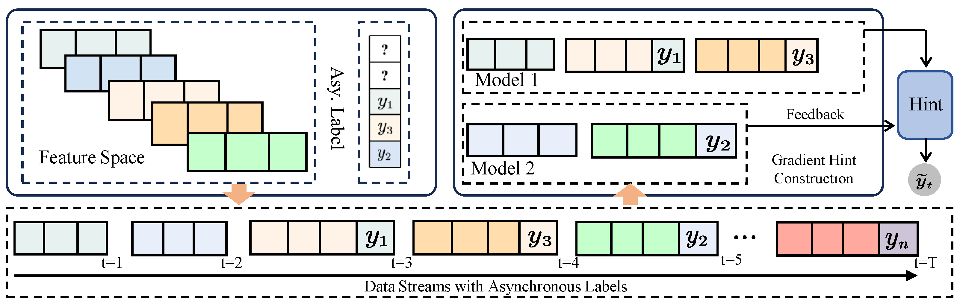
To overcome this limitation, we propose a general-purpose solution based on gradient hint construction, the general principle of which is shown in Figure 2. At each time t, the learner forms a surrogate gradient vector h t R m , which approximates the true gradient t ( ω t ) = ω ( f ( ω t , x ^ t ) , y t ) using partially observed information. The model is then updated via a proximal step:
ω t + 1 * = arg min ω W h t , ω + 1 2 η | ω ω t | 2 ,
where W R m is a compact convex feasible set, and · , · denotes the standard inner product.
This update can be interpreted as an implicit Euler step over a linearized surrogate loss, balancing descent direction h t with proximity to the current model ω t . When the actual label y t becomes available, the learner can retroactively refine h t , or use it to update future hints. This mechanism naturally interpolates between different feedback regimes: when h t = t ( ω t ) , it recovers full-information gradient descent; when h t = 0 , it performs no update. Such flexibility enables learning under irregular, delayed, and partial supervision, which are common in streaming and edge intelligence settings.
  • Construction and Regret Analysis of Hint Gradients. The construction of the hint vector h t R m is the core mechanism that enables learning under delayed supervision in the OALN algorithm. At each time step t, the learner must determine how to approximate the true loss gradient t ( ω t ) , despite potentially missing parts of the instance–label pair ( x ^ t , y t ) . The strategy for computing h t depends on which elements are currently available.
When the feature vector x ^ t is observed but the label y t has not yet arrived, we estimate a soft pseudo-label y ˜ t [ 1 , + 1 ] using an ensemble of previously deployed models { ω s } s < t , such as via confidence-weighted majority voting or exponential decay averaging [51]. Concretely, each model ω s is assigned a confidence weight:
w s , t exp γ L s ( t ) ,
where L s ( t ) denotes the cumulative loss of model s over a sliding window up to time t, and γ > 0 is a decay parameter. These weights are then normalized, and updated online after each labeled feedback via exponential smoothing:
w s , t α w s , t 1 + ( 1 α ) exp γ ( f ( ω s , x ^ t ) , y t ) , α ( 0 , 1 )
where α is a smoothing coefficient that governs the trade-off between the prior confidence w s , t 1 and the newly observed loss-based weight. This scheme ensures that higher-performing models contribute more strongly to y ˜ t , while poor performers are gradually down-weighted.
The surrogate gradient is then computed using
h t = * ( f ( ω t , x ^ t ) , y ˜ t ) ,
where f ( ω , x ^ ) R is the prediction function, and : R × { 1 , + 1 } R + is a convex loss.
Alternatively, when only the label y t is received and the corresponding features x ^ t are missing, we approximate the input using a class-wise prototype:
μ y t = 1 | H y t | s H y t x ^ s ,
where H y = { s < t y s = y } denotes the historical index set for label y. The hint gradient is computed as
h t = ( f ( ω t , μ y t ) , y t ) .
In the case where both x ^ t and y t are unavailable at time t, the learner defers the update entirely, or adopts a temporal smoothing strategy such as reusing the previous update direction h t = h t 1 . This ensures continuity in learning while awaiting supervision.
To formally analyze the performance impact of hint-based updates, we consider the cumulative regret after T steps:
R t = t = 1 T t ( ω t ) min ω W t = 1 T t ( ω ) ,
where t ( ω ) = ( f ( ω , x ^ t ) , y t ) if the label is eventually received, and W R m is a convex, bounded parameter space.
We assume that (i) the loss t is convex and L-Lipschitz in ω ; (ii) each hint satisfies h t t ( ω t ) ε t ; and (iii) the hypothesis space has the following diameter:
D = max ω , ω | ω ω | .
Then, the expected regret is bounded by
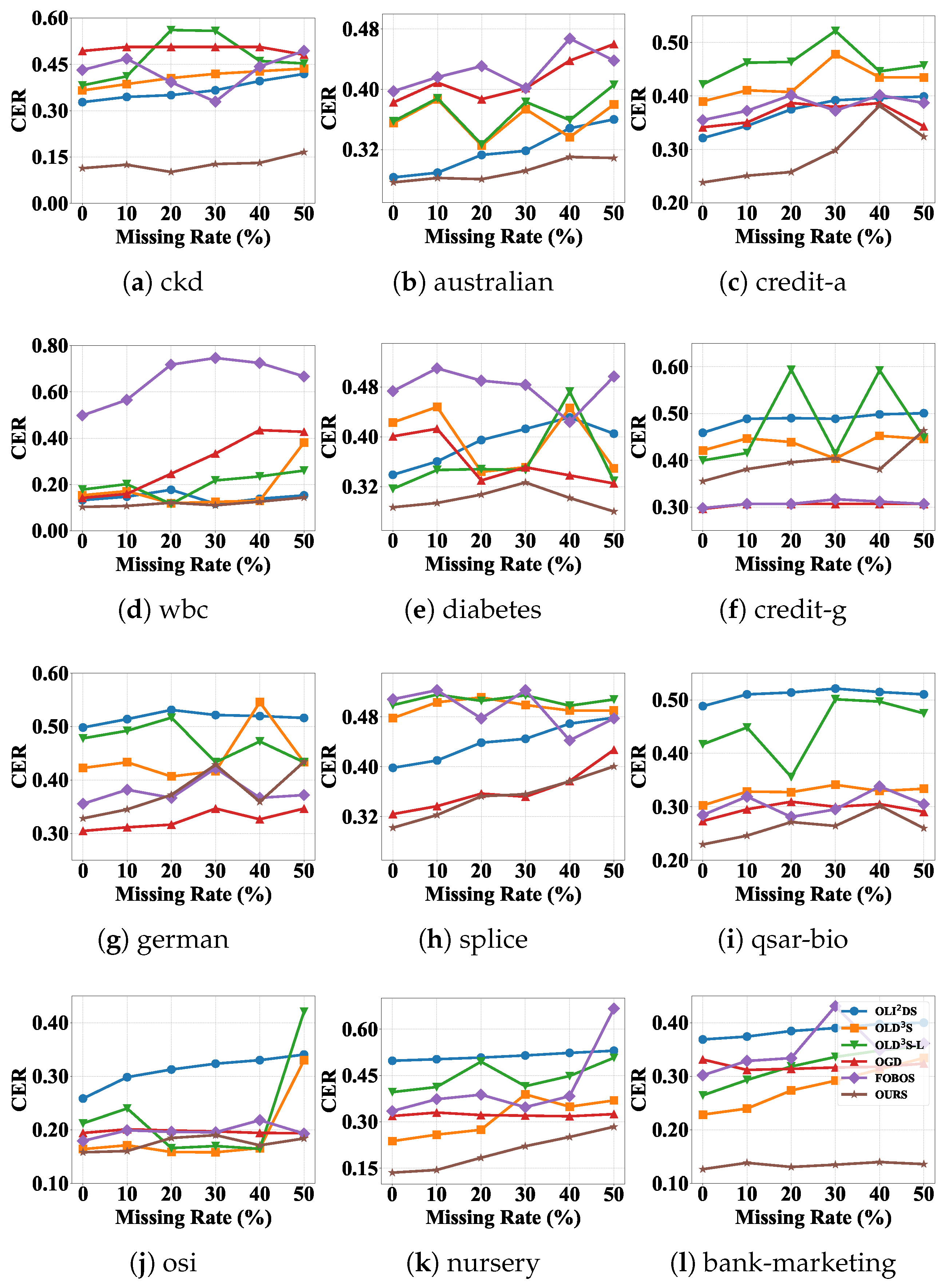
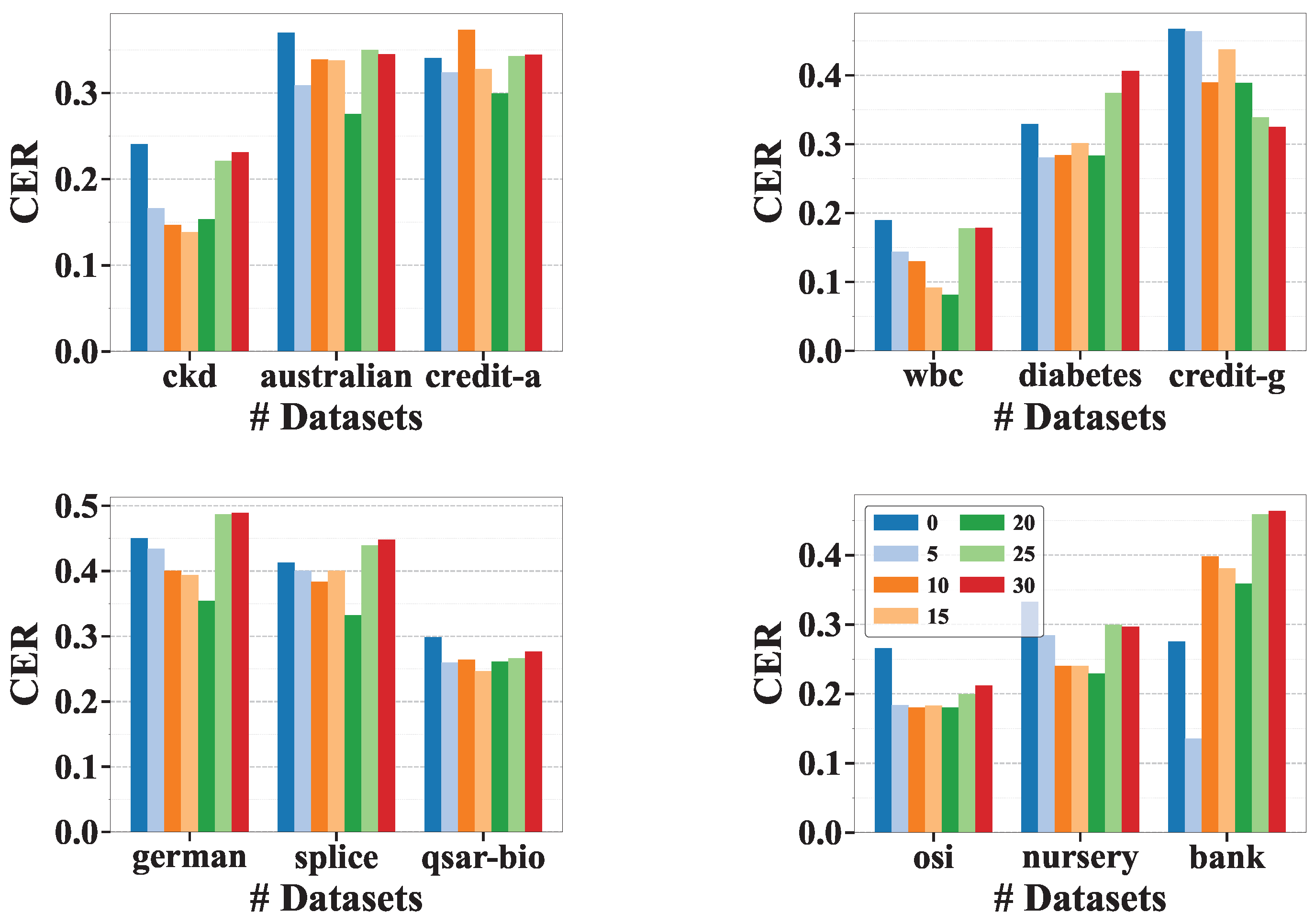
E [ R T ] D 2 2 η + η 2 t = 1 T | h t | 2 + D t = 1 T ε t .
Choosing η = O ( 1 / T ) and ε t = O ( 1 / T ) yields E [ R T ] = O ( T ) , confirming that the OALN algorithm achieves no-regret learning even with approximate supervision.
This result demonstrates that as long as hint gradients approximate the true gradients with bounded error, the model remains competitive. Coupled with the latent feature imputation from Section 4.1, our framework provides a principled approach to online learning under dual uncertainty: incomplete inputs and delayed feedback.

4.3. Discussion

  • Algorithm Design and Analysis. The OALN algorithm addresses incomplete mixed nominal–numeric inputs and asynchronous label feedback in real-time streams by combining Gaussian Copula-based latent encoding, conditional imputation, adaptive gradient updates, and hint-guided model refinement within a unified streaming framework, the schematic diagram is shown in the Algorithm 1. At each time step t, a partially observed instance x t = ( x t nom , x t num ) is mapped into a latent representation z t R D . Missing entries are filled via conditional expectation under current copula parameters ( μ , Σ ) , and the completed vector is inverted back to the original feature space. OALN maintains two queues— Q all (model pool) and Q ready (ready-to-update models). Upon arrival of delayed labels y t d , corresponding historical models execute supervised proximal gradient updates; otherwise, OALN synthesizes surrogate gradients from an ensemble-derived hint vector, ensuring uninterrupted learning despite feedback latency. Our theoretical analysis bounds per-step time complexity by O ( D 3 + N t D ) and memory by O ( D 2 + N max D + B D ) . In practical settings where the number of missing values M D , imputation cost reduces to O ( M 3 + M 2 + M D ) . Scalability is further enhanced through rank-one copula updates, low-rank ( r D ) or diagonal copula approximations that reduce storage to O ( D r ) , dynamic pruning of stale models to bound N t , and parallel hint generation across multi-core resources. Low-rank copula approximation compresses the full covariance matrix by keeping only its principal directions, cutting both memory and computation costs while retaining the essential correlation structure—this makes online copula updates much faster and more scalable without sacrificing accuracy. These optimizations render OALN both memory-efficient and computationally tractable in high-dimensional, irregularly delayed streaming environments.For more details on algorithm design and analysis, please refer to Appendix B.
  • Edge Deployment and Model Slimming. To support deployment on resource-constrained edge devices, we apply a combination of techniques: compressing the copula covariance via low-rank or diagonal approximations to reduce storage from O ( D 2 ) to O ( D r ) ; pruning stale models to limit the model pool memory to O ( N t D ) ; performing incremental rank-one updates at O ( D r ) per step instead of full matrix recomputations; and tuning the delayed-label buffer to a small window b B , yielding O ( b D ) overhead. With r , b D and aggressively pruned N t , total memory can shrink to O ( D r + N t D + b D ) , making OALN feasible within typical edge budgets. We believe this concrete guidance will facilitate real-world, on-device deployment of OALN.
Algorithm 1: The OALN Algorithm
Bdcc 09 00177 i001
  • Algorithm Limitation. OALN still relies on fixed-width bins to incrementally update the empirical CDF and to estimate the Gaussian Copula correlation matrix. Under high missingness or when most feature values are zero, many bins remain empty, producing a coarse, step-like CDF and highly noisy correlation estimates. This noise undermines the stability of the latent variables and degrades the accuracy of subsequent online model updates. Moreover, once bin boundaries are fixed they cannot adapt to distributional drift, limiting OALN’s effectiveness on high-cardinality or rapidly changing sparse features. OALN’s model pool scheduling and weighting depend solely on the “old” labels that have arrived. When label delays are heavy-tailed, bursty, or excessively long, the noise in performance estimates rises sharply, causing incorrect model switches and accumulated prediction errors. At the same time, feedback latency severely impairs the algorithm’s ability to detect and adapt to concept drift, constraining real-time responsiveness and robustness in live streaming environments.

5. Experiments

This section presents the experiments conducted to address the following research questions, which collectively evaluate the effectiveness of the OALN algorithm:
  • RQ1: Under varying missing rates, does OALN outperform other methods?
  • RQ2: How does the performance of OALN and baseline algorithms change as the missing rate increases?
  • RQ3: Under different levels of asynchronous label arrival, how does OALN perform, and what performance trends emerge in comparison to other methods?

5.1. General Setting

  • Dataset. We evaluate OALN on twelve real-world datasets spanning a wide range of application domains [52]. To simulate dynamic feature spaces, we introduce random missingness at varying rates. Table 2 summarizes the key characteristics of these datasets.
  • Evaluation Metrics. We adopt the cumulative error rate (CER) as one of the evaluation metrics to quantify classification errors in online learning. CER is widely used in prior work [17,35] and is defined as
    CER = 1 N j < N y j sign ( y ˜ j ) ,
    where N denotes the total number of samples, and the angle-bracket notation · evaluates to 1 if the condition inside is true, and to 0 otherwise. A lower CER indicates better model performance.
We use the Area Under the Receiver Operating Characteristic Curve (AUC) to evaluate the ability of a binary classifier to distinguish between positive and negative samples [53]. AUC is widely applied in domains such as medical diagnosis, credit scoring, and other decision-critical tasks [54]. It is defined as
AUC = 0 1 TPR FPR 1 ( x ) d x ,
where FPR (false-positive rate) is the ROC curve’s horizontal axis and TPR (true-positive rate) is its vertical axis. AUC equals the area under this curve; values closer to 1 indicate stronger discriminative power and better model performance.
  • Compared Methods. We compare OALN with five related algorithms. Brief descriptions of each are provided below:
    • OLI2DS [14]: An online learning algorithm that operates over varying feature subsets by adaptively weighting incomplete subspaces. It integrates dynamic cost strategies and sparse online updates to enhance model performance on complex data streams.
    • OLD3S [55]: A deep learning-based method that employs parallel dual models, dynamic fusion, and autoencoder-based regularization to improve robustness and stability under streaming conditions.
    • OLD3S-L [55]: A lightweight variant of OLD3S that retains the dynamic fusion mechanism while reducing encoding depth and fusion dimensionality, significantly decreasing model size and online update complexity for resource-constrained environments.
    • OGD [56]: A classical online learning algorithm that updates model weights based on the gradient of each incoming sample, using a time-decaying step size to ensure simplicity and efficiency.
    • FOBOS [57]: An online method that combines gradient descent with regularization, enabling incremental updates while encouraging model sparsity through penalization of irrelevant features.
  • Implementation Details. To ensure fairness in our experiments, we employ a random-removal strategy, independently removing 10% and 50% of instances from each of the eleven datasets. Simultaneously, we set the learning rate to 0.3, the number of training epochs to 30, and the optimizer’s weight factors to β 1 = 0.1 and β 2 = 0.9 . The batch size is defined as one-thirtieth of the feature dimensionality, the test set size is 1024, and the number of solver iterations is set to 200. At the same time, we also set the random seed = 2025. This procedure generates nonstationary data streams while ensuring that all models receive identical input sequences. We assume a Missing Completely At Random (MCAR) mechanism for all removals [48].

5.2. Performance Comparison (RQ1)

Based on the results in Table 3, Table 4, Table 5 and Table 6, which report the cumulative error rate (CER) and AUC scores for each algorithm under 10% and 50% missing rates (with label delay T = 5 for OALN), we perform statistical analyses utilizing the win/loss ratio, alongside the Wilcoxon signed-rank test (p-value) [58]. First, our algorithm demonstrates consistently strong performance: at a 10% missing rate, the average CER across the eleven datasets is 23.31%, and at a 50% missing rate, it is 28.28%—both lower than the corresponding averages of the baseline methods. Moreover, across the 60 total evaluation scenarios, OALN achieves a lower CER than all competing algorithms in 57 scenarios at 10% missingness and in 52 scenarios at 50% missingness. Second, regarding AUC scores in the same 60 scenarios, OALN outperforms all competitors in 57 scenarios at 10% missingness and in 58 scenarios at 50% missingness. The mean AUC values achieved by OALN are 0.7895 at 10% missingness and 0.7433 at 50% missingness, both higher than the corresponding averages of the comparison methods. These results indicate that by constructing a hybrid feature space combining nominal and numerical data, OALN maintains high predictive accuracy and stability under nonstationary data streams and asynchronous label feedback. Furthermore, our experiments confirm that the use of a mixed Gaussian Copula—through online estimation of joint nominal–numerical distributions and conditional imputation of missing values—significantly enhances predictive performance under various missingness patterns.

5.3. Trend Comparison (RQ2)

By comparing OLI2DS, OLD3S, OLD3S-L, OGD, and FOBOS, we draw the following conclusions. To analyze how each algorithm’s performance varies with different missing rates, Figure 3 presents the CER curves for all methods under the nonstationary setting, with label delay T = 5 for OALN.
As the missing rate increases, OALN’s CER remains lower than that of the other algorithms in most cases; in Figure 3a, OALN outperforms its competitors in over 55% of the scenarios. Overall, the CER values for all methods tend to increase as the missingness rate rises. Furthermore, Figure 3e,f,j reveal that OLD3S-L exhibits large CER oscillations on certain datasets as the missing rate grows. This behavior arises because OLD3S-L employs only a shallow autoencoder, which can marginally recover major features at low missing rates; however, when the missing rate reaches 30%, 40%, or higher, essential feature information is severely lost, and the shallow network fails to accurately reconstruct or denoise the data. Consequently, noise in the imputed features is directly propagated to the classifier, resulting in pronounced fluctuations in CER. In Figure 3d, we observe that FOBOS’s CER is markedly higher than that of the other methods. This is because FOBOS assumes a fixed and complete feature space and lacks a mechanism for adapting to dynamically changing feature dimensions. When features are missing, its parameter updates rely on incomplete or erroneous input distributions, leading to rapid error accumulation. Moreover, in missing-data scenarios, leveraging the covariance structure among observed features is critical for effective imputation. FOBOS, however, applies regularization only in the parameter space and entirely disregards feature-level correlations, rendering it incapable of inferring missing values from the available features. Similarly, in Figure 3j–k, OLI2DS exhibits higher CER than the other algorithms in most cases, suggesting that its accuracy degrades on larger or more complex datasets.
To assess whether OALN encounters similar issues, we present in Figure 4 bar charts showing OALN’s CER at different missing rates (with label delay T = 5 ), in order to further analyze its robustness under increasing missingness. As shown in Figure 4, the CER values for all datasets increase steadily with rising missing rates, yet remain relatively stable without significant oscillations, and outperform the competing methods in most cases. Notably, on large-scale datasets such as osi and nursery, OALN maintains consistently strong performance. These findings demonstrate that our conditional covariance-based adaptive imputation mechanism, combined with incremental copula parameter updates for dynamic feature space adaptation, effectively addresses both feature missingness and large-sample scenarios, thereby ensuring the model’s accuracy, robustness, and overall superiority.

5.4. Asynchronous Label Processing (RQ3)

To answer RQ3, we fix the missing rate at 50% and simulate asynchronous label feedback by varying the delay intensity T { 0 , 5 , 10 , 15 , 20 , 25 , 30 } . Figure 5 shows that as the label delay T increases, the cumulative error rate (CER) decreases initially and then increases, with an inflection point at approximately T = 20 . When labels are delayed, OALN continues to receive and process additional feature samples before the true label y t becomes available, performing incremental updates of the copula parameters μ and Σ at each step. Longer delays incorporate more samples into the covariance estimation and feature imputation processes, yielding more stable estimates of both the covariance matrix and the mean vector, as well as higher-quality imputations. This leads to more accurate input features for the classifier, reduces misclassification, and lowers the overall CER. Furthermore, for T > 0 , each incoming sample—even without an associated true label—triggers a hint update: a pseudo-label generated by the ensemble of existing submodels in the model pool, followed by a gradient update. With longer delays, the number of hint-based updates increases, offering the model additional opportunities to smooth ensemble weights and correct predictive biases. By the time the true label arrives, the model has already transitioned to a better parameter region, rendering subsequent gradient updates more robust.
However, as the delay intensity T continues to increase, its adverse impact on the model gradually outweighs the mechanisms described above, causing the cumulative error rate (CER) to halt its decline and begin to increase.
In summary, appropriate label delays act as a “warm-up” mechanism for OALN, enabling comprehensive covariance estimation, improved imputation, and pseudo-label refinement prior to receiving true-label feedback. However, as the delay intensity T continues to increase, the model begins to suffer from the negative effects of the delay, leading to a decline in performance. Consequently, there exists an “equilibrium point” between model performance and delay intensity: before this point, the model can maintain a low cumulative error rate (CER) when the true labels eventually arrive; after this point, the model’s CER gradually increases.

6. Conclusions

In this study, we address the modeling challenges posed by nominal and numerical features under conditions of feature missingness and asynchronous label feedback in online learning. Data streams arrive in real time with heterogeneous and dynamically evolving feature types, which can significantly impair model accuracy and robustness. To mitigate these issues, we propose the Online Asynchronous Learning over Streaming Nominal Data (OALN) algorithm. OALN leverages a mixed Gaussian Copula to dynamically capture correlations among features and incorporates a model pool with a hint mechanism to ensure data integrity, stability, and accuracy in the presence of missing values, heterogeneous features, and delayed labels. Experimental results show that OALN consistently achieves high predictive accuracy across varying missing rates and delay intensities, outperforming competing methods. These advances highlight OALN’s potential for effectively handling heterogeneous, incomplete, and asynchronously labeled data in real-time online learning scenarios.
By virtue of its robust handling of incomplete mixed-type data and asynchronous feedback, OALN is well suited for real-time streaming applications such as industrial IoT, smart grids, energy management, and online financial risk control. Although OALN handles moderate missingness and fixed delays, its reliance on static, bin-based CDF updates produces step-like distributions and noisy copula correlations under high feature sparsity, while depending solely on delayed labels for model selection introduces estimation noise and impairs concept-drift adaptation. In this work, we simulate feature dropout under the MCAR assumption, where missingness is independent of both observed and unobserved data. While simplifying the evaluation, this may overestimate imputation and learning performance. Future work will consider MAR and MNAR settings to more fully assess robustness under realistic missing-data mechanisms. We will also investigate adaptive distribution summaries (e.g., sketch-based or dynamic binning), develop delay-aware weighting schemes and integrated drift-detection mechanisms, and design robust, adaptive techniques to handle non-MCAR missing data, all aimed at improving robustness and real-time responsiveness in highly sparse, irregularly delayed streaming environments.

Author Contributions

Conceptualization, H.L. and S.Z.; methodology, S.Z. and L.L.; software, J.C. and T.W.; validation, H.L., S.Z. and S.L.; formal analysis, S.Z.; investigation, H.L. and J.C.; resources, S.Z.; data curation, L.L.; writing—original draft preparation, S.Z.; writing—review and editing, H.L., J.T. and S.H.; visualization, T.W.; supervision, S.H.; project administration, S.H.; funding acquisition, S.H. All authors have read and agreed to the published version of the manuscript.

Funding

This work was supported by Jinan University, the National Natural Science Foundation of China (No.62272198), Guangdong Key Laboratory of Data Security and Privacy Preserving (No. 2023B1212060036), Guangdong–Hong Kong Joint Laboratory for Data Security and Privacy Preserving (No. 2023B1212120007), Guangdong Basic and Applied Basic Research Foundation under Grant (No. 2024A1515010121), and the Special Funds for the Cultivation of Guangdong College Students’ Scientific and Technological Innovation (Climbing Program Special Funds) under Grant pdjh2025ak028.

Data Availability Statement

Conflicts of Interest

The authors declare no conflicts of interest. The funders had no role in the design of the study; in the collection, analyses, or interpretation of data; in the writing of the manuscript; or in the decision to publish the results.

Appendix A

As shown in Table A1, Table A2, Table A3, Table A4, Table A5, Table A6, Table A7 and Table A8, even at missing rates of 0%, 20%, 30%, and 40% with label delay T = 5, our OALN algorithm consistently delivers superior performance in both cumulative error rate (CER) and AUC. Compared to all baseline methods, OALN achieves the lowest average CER and the highest average AUC score across these missingness levels.
Table A1. Cumulative error rate (CER) under the missing rate 0% with label delay T = 5. The best results are in bold. • indicates the cases in our method that lose the comparison. * shows the total number of wins and losses for OALN.
DatasetOLI2DSOLD3SOLD3S-LOGDFOBOSOALN
ckd 0.3276 ± 0.003 0.3655 ± 0.012 0.3821 ± 0.002 0.4933 ± 0.006 0.4316 ± 0.022 0 . 1138 ± 0 . 002
australian 0.2832 ± 0.005 0.3551 ± 0.003 0.3575 ± 0.019 0.3826 ± 0.011 0.3974 ± 0.004 0 . 2766 ± 0 . 001
credit-a 0.3213 ± 0.014 0.3899 ± 0.003 0.4218 ± 0.009 0.3414 ± 0.004 0.3549 ± 0.020 0 . 2382 ± 0 . 006
wbc 0.1324 ± 0.003 0.1538 ± 0.007 0.1782 ± 0.001 0.1421 ± 0.010 0.4982 ± 0.004 0 . 1033 ± 0 . 002
diabetes 0.3392 ± 0.004 0.4231 ± 0.015 0.3166 ± 0.003 0.4008 ± 0.002 0.4733 ± 0.004 0 . 2871 ± 0 . 010
credit-g 0.4587 ± 0.010 0.4210 ± 0.003 0.3994 ± 0.011 0.2958 ± 0.019 0.2977 ± 0.015 0.3551 ± 0.020
german 0.4983 ± 0.008 0.4226 ± 0.022 0.4780 ± 0.014 0.3048 ± 0.010 0.3556 ± 0.006 0.3283 ± 0.014
splice 0.3982 ± 0.003 0.4779 ± 0.021 0.4987 ± 0.006 0.3240 ± 0.004 0.5082 ± 0.010 0 . 3021 ± 0 . 006
qsar-bio 0.4882 ± 0.014 0.3025 ± 0.003 0.4169 ± 0.005 0.2733 ± 0.023 0.2846 ± 0.014 0 . 2295 ± 0 . 002
osi 0.2583 ± 0.003 0.1636 ± 0.012 0.2118 ± 0.016 0.1939 ± 0.008 0.1790 ± 0.011 0 . 1577 ± 0 . 009
nursery 0.4977 ± 0.004 0.2374 ± 0.010 0.3962 ± 0.007 0.3188 ± 0.001 0.3348 ± 0.013 0 . 1356 ± 0 . 002
bank-marketing 0.3688 ± 0.005 0.2282 ± 0.007 0.2643 ± 0.010 0.3313 ± 0.005 0.3018 ± 0.005 0 . 1261 ± 0 . 003
loss/win 0 / 12 1 / 11 1 / 11 2 / 10 1 / 11 5 / 55 *
p-value 0.0005 0.0005 0.0005 0.0122 0.0034
F-rank 4.167 3.583 4.417 3.250 4.333 1.250
Table A2. AUC under missing rate 0% with label delay T = 5. The best results are in bold. • indicates the cases in our method that lose the comparison. * shows the total number of wins and losses for OALN.
DatasetOLI2DSOLD3SOLD3S-LOGDFOBOSOALN
ckd 0.7382 ± 0.003 0.5922 ± 0.011 0.5484 ± 0.003 0.4796 ± 0.005 0.8566 ± 0.003 0 . 9330 ± 0 . 002
australian 0.7924 ± 0.004 0.5980 ± 0.003 0.6133 ± 0.014 0.6569 ± 0.010 0.6331 ± 0.002 0 . 8353 ± 0 . 004
credit-a 0.7210 ± 0.014 0.5832 ± 0.005 0.4921 ± 0.004 0.6883 ± 0.010 0.6521 ± 0.018 0 . 8069 ± 0 . 003
wbc 0.9233 ± 0.009 0.7508 ± 0.006 0.6582 ± 0.003 0.9433 ± 0.023 0.9859 ± 0.004 0 . 9877 ± 0 . 007
diabetes 0.7036 ± 0.006 0.5599 ± 0.011 0.5743 ± 0.004 0.6582 ± 0.004 0.4931 ± 0.011 0 . 7535 ± 0 . 005
credit-g 0.5262 ± 0.012 0.5004 ± 0.005 0.5136 ± 0.010 0.4823 ± 0.010 0.4592 ± 0.005 0 . 6321 ± 0 . 011
german 0.4973 ± 0.014 0.6032 ± 0.009 0.5421 ± 0.009 0.7432 ± 0.006 0.5721 ± 0.014 0.7328 ± 0.008
splice 0.6392 ± 0.006 0.5273 ± 0.013 0.5329 ± 0.009 0.7904 ± 0.005 0.6053 ± 0.013 0.7642 ± 0.003
qsar-bio 0.4921 ± 0.013 0.6125 ± 0.006 0.5583 ± 0.013 0.7849 ± 0.010 0.6656 ± 0.005 0 . 8377 ± 0 . 003
osi 0.7913 ± 0.004 0.7013 ± 0.013 0.5681 ± 0.021 0.3677 ± 0.011 0.3585 ± 0.003 0.7182 ± 0.005
nursery 0.5182 ± 0.017 0.7811 ± 0.005 0.5635 ± 0.009 0.7399 ± 0.014 0.5291 ± 0.006 0 . 9038 ± 0 . 004
bank-marketing 0.7607 ± 0.002 0.6634 ± 0.004 0.6321 ± 0.005 0.6207 ± 0.006 0.4441 ± 0.002 0 . 7685 ± 0 . 001
loss/win 1 / 10 0 / 11 0 / 11 1 / 10 0 / 11 2 / 53 *
p-value 0.0049 0.0005 0.0005 0.0024 0.0005
F-rank 3.250 4.167 4.667 3.250 4.250 1.417
Table A3. Cumulative error rate (CER) under missing rate 20% with label delay T = 5. The best results are in bold. • indicates the cases in our method that lose the comparison. * shows the total number of wins and losses for OALN.
DatasetOLI2DSOLD3SOLD3S-LOGDFOBOSOALN
ckd 0.3503 ± 0.010 0.4056 ± 0.008 0.5611 ± 0.005 0.5063 ± 0.008 0.3924 ± 0.022 0 . 1015 ± 0 . 005
australian 0.3130 ± 0.007 0.3253 ± 0.005 0.3269 ± 0.023 0.3869 ± 0.011 0.4307 ± 0.005 0 . 2808 ± 0 . 003
credit-a 0.3750 ± 0.013 0.4074 ± 0.003 0.4638 ± 0.012 0.3869 ± 0.005 0.4015 ± 0.018 0 . 2577 ± 0 . 005
wbc 0.1773 ± 0.005 0.1190 ± 0.004 0.1159 ± 0.003 0.2464 ± 0.010 0.7174 ± 0.004 0.1213 ± 0.002
diabetes 0.3949 ± 0.004 0.3439 ± 0.016 0.3483 ± 0.005 0.3301 ± 0.003 0.4901 ± 0.002 0 . 3074 ± 0 . 011
credit-g 0.4901 ± 0.011 0.4389 ± 0.003 0.5933 ± 0.017 0.3065 ± 0.021 0.3065 ± 0.018 0.3954 ± 0.025
german 0.5312 ± 0.011 0.4067 ± 0.018 0.5167 ± 0.012 0.3166 ± 0.014 0.3668 ± 0.007 0.3723 ± 0.011
splice 0.4385 ± 0.005 0.5111 ± 0.014 0.5056 ± 0.007 0.3568 ± 0.005 0.4774 ± 0.008 0 . 3526 ± 0 . 005
qsar-bio 0.5138 ± 0.011 0.3274 ± 0.003 0.3558 ± 0.001 0.3095 ± 0.019 0.2810 ± 0.010 0 . 2714 ± 0 . 002
osi 0.3126 ± 0.003 0.1582 ± 0.011 0.1656 ± 0.016 0.1984 ± 0.008 0.1959 ± 0.010 0.1845 ± 0.006
nursery 0.5080 ± 0.004 0.2743 ± 0.008 0.4948 ± 0.009 0.3219 ± 0.004 0.3879 ± 0.013 0 . 1836 ± 0 . 003
bank-marketing 0.3846 ± 0.004 0.2733 ± 0.002 0.3182 ± 0.003 0.3138 ± 0.008 0.3339 ± 0.003 0 . 1303 ± 0 . 002
loss/win 0 / 12 2 / 10 2 / 10 2 / 10 2 / 10 8 / 52 *
p-value 0.0005 0.0024 0.0024 0.0269 0.0049
F-rank 4.333 3.500 4.417 3.208 3.958 1.583
Table A4. AUC under missing rate 20% with label delay T = 5. The best results are in bold. • indicates the cases in our method that lose the comparison. * shows the total number of wins and losses for OALN.
DatasetOLI2DSOLD3SOLD3S-LOGDFOBOSOALN
ckd 0.7194 ± 0.002 0.5479 ± 0.013 0.4946 ± 0.002 0.3756 ± 0.004 0.7192 ± 0.002 0 . 9387 ± 0 . 001
australian 0.7426 ± 0.004 0.6854 ± 0.002 0.6660 ± 0.009 0.6325 ± 0.014 0.5853 ± 0.004 0 . 7873 ± 0 . 005
credit-a 0.6580 ± 0.011 0.5647 ± 0.005 0.4681 ± 0.004 0.6614 ± 0.010 0.6674 ± 0.015 0 . 7970 ± 0 . 003
wbc 0.8774 ± 0.008 0.9169 ± 0.005 0.9002 ± 0.003 0.7623 ± 0.016 0.9788 ± 0.005 0 . 9809 ± 0 . 004
diabetes 0.6401 ± 0.006 0.5211 ± 0.009 0.5602 ± 0.007 0.5446 ± 0.005 0.3857 ± 0.013 0 . 6785 ± 0 . 005
credit-g 0.5150 ± 0.023 0.4994 ± 0.006 0.4805 ± 0.010 0.4455 ± 0.007 0.4538 ± 0.008 0 . 6025 ± 0 . 011
german 0.4631 ± 0.016 0.6065 ± 0.008 0.5062 ± 0.010 0.6613 ± 0.008 0.4916 ± 0.013 0 . 6743 ± 0 . 011
splice 0.5823 ± 0.008 0.4953 ± 0.011 0.4851 ± 0.009 0.7617 ± 0.007 0.5987 ± 0.014 0.7312 ± 0.003
qsar-bio 0.4659 ± 0.013 0.6306 ± 0.006 0.5616 ± 0.014 0.6981 ± 0.006 0.6186 ± 0.005 0 . 8333 ± 0 . 001
osi 0.7442 ± 0.007 0.5849 ± 0.010 0.5155 ± 0.020 0.3545 ± 0.014 0.3394 ± 0.002 0.6985 ± 0.003
nursery 0.4926 ± 0.015 0.6709 ± 0.006 0.5444 ± 0.009 0.6677 ± 0.011 0.5757 ± 0.003 0 . 8693 ± 0 . 005
bank-marketing 0.7116 ± 0.005 0.6022 ± 0.003 0.5933 ± 0.006 0.5044 ± 0.007 0.4984 ± 0.002 0 . 7376 ± 0 . 002
loss/win 1 / 11 0 / 12 0 / 12 1 / 11 0 / 12 2 / 58 *
p-value 0.0034 0.0005 0.0005 0.0015 0.0005
F-rank 3.500 3.500 4.500 4.000 4.333 1.167
Table A5. Cumulative error rate (CER) under missing rate 30% with label delay T = 5. The best results are in bold. • indicates the cases in our method that lose the comparison. * shows the total number of wins and losses for OALN.
DatasetOLI2DSOLD3SOLD3S-LOGDFOBOSOALN
ckd 0.3660 ± 0.013 0.4194 ± 0.007 0.5583 ± 0.003 0.5063 ± 0.010 0.3291 ± 0.018 0 . 1273 ± 0 . 005
australian 0.3184 ± 0.009 0.3736 ± 0.003 0.3833 ± 0.020 0.4015 ± 0.012 0.4015 ± 0.004 0 . 2920 ± 0 . 004
credit-a 0.3920 ± 0.009 0.4783 ± 0.004 0.5217 ± 0.013 0.3796 ± 0.007 0.3723 ± 0.020 0 . 2982 ± 0 . 003
wbc 0.1170 ± 0.003 0.1254 ± 0.007 0.2175 ± 0.005 0.3333 ± 0.007 0.7464 ± 0.008 0 . 1104 ± 0 . 001
diabetes 0.4128 ± 0.005 0.3512 ± 0.015 0.3468 ± 0.005 0.3512 ± 0.005 0.4834 ± 0.003 0 . 3269 ± 0 . 012
credit-g 0.4887 ± 0.011 0.4033 ± 0.003 0.4144 ± 0.017 0.3065 ± 0.021 0.3166 ± 0.018 0.4046 ± 0.025
german 0.5217 ± 0.009 0.4167 ± 0.019 0.4333 ± 0.007 0.3467 ± 0.016 0.4221 ± 0.005 0.4287 ± 0.010
splice 0.4447 ± 0.006 0.4989 ± 0.012 0.5144 ± 0.009 0.3518 ± 0.006 0.5226 ± 0.007 0 . 3559 ± 0 . 003
qsar-bio 0.5211 ± 0.013 0.3411 ± 0.002 0.5011 ± 0.001 0.3000 ± 0.018 0.2952 ± 0.012 0 . 2642 ± 0 . 001
osi 0.3235 ± 0.004 0.1577 ± 0.010 0.1694 ± 0.015 0.1968 ± 0.011 0.1951 ± 0.006 0.1898 ± 0.005
nursery 0.5149 ± 0.004 0.3889 ± 0.007 0.4154 ± 0.010 0.3200 ± 0.006 0.3474 ± 0.015 0 . 2211 ± 0 . 002
bank-marketing 0.3901 ± 0.004 0.2916 ± 0.005 0.3361 ± 0.004 0.3163 ± 0.006 0.4311 ± 0.003 0 . 1345 ± 0 . 003
loss/win 0 / 12 3 / 9 1 / 11 3 / 9 2 / 10 9 / 51 *
p-value 0.0005 0.0122 0.0034 0.0522 0.0093
F-rank 4.500 3.292 4.333 3.167 3.958 1.750
Table A6. AUC under missing rate 30% with label delay T = 5. The best results are in bold. • indicates the cases in our method that lose the comparison. * shows the total number of wins and losses for OALN.
DatasetOLI2DSOLD3SOLD3S-LOGDFOBOSOALN
ckd 0.7037 ± 0.004 0.6079 ± 0.011 0.6970 ± 0.003 0.4026 ± 0.005 0.7333 ± 0.004 0 . 9374 ± 0 . 002
australian 0.7336 ± 0.004 0.5578 ± 0.004 0.7187 ± 0.010 0.5788 ± 0.012 0.6117 ± 0.003 0 . 8227 ± 0 . 006
credit-a 0.6370 ± 0.010 0.5086 ± 0.006 0.5829 ± 0.002 0.6229 ± 0.008 0.5652 ± 0.012 0 . 7892 ± 0 . 004
wbc 0.9143 ± 0.009 0.9151 ± 0.002 0.6810 ± 0.005 0.9165 ± 0.014 0.9811 ± 0.007 0 . 9843 ± 0 . 003
diabetes 0.6092 ± 0.008 0.5189 ± 0.006 0.5019 ± 0.003 0.5017 ± 0.006 0.4077 ± 0.015 0 . 6652 ± 0 . 003
credit-g 0.5180 ± 0.019 0.5046 ± 0.008 0.5312 ± 0.011 0.4454 ± 0.005 0.4451 ± 0.004 0 . 5929 ± 0 . 009
german 0.4733 ± 0.014 0.5898 ± 0.009 0.5563 ± 0.011 0.6510 ± 0.005 0.5315 ± 0.013 0.6064 ± 0.010
splice 0.5750 ± 0.009 0.5040 ± 0.013 0.5017 ± 0.004 0.7231 ± 0.008 0.6205 ± 0.013 0.7177 ± 0.006
qsar-bio 0.4607 ± 0.011 0.5578 ± 0.009 0.5727 ± 0.016 0.6522 ± 0.009 0.5906 ± 0.004 0 . 8181 ± 0 . 002
osi 0.7144 ± 0.005 0.6252 ± 0.013 0.6037 ± 0.017 0.3849 ± 0.016 0.3682 ± 0.005 0.6488 ± 0.002
nursery 0.4873 ± 0.013 0.6618 ± 0.008 0.8048 ± 0.005 0.6197 ± 0.013 0.4881 ± 0.006 0 . 8442 ± 0 . 003
bank-marketing 0.6988 ± 0.006 0.6007 ± 0.002 0.5829 ± 0.006 0.4658 ± 0.003 0.5266 ± 0.003 0 . 7340 ± 0 . 002
loss/win 1 / 11 0 / 12 0 / 12 2 / 10 0 / 12 3 / 57 *
p-value 0.0024 0.0005 0.0005 0.0024 0.0005
F-rank 3.500 4.250 3.833 3.833 4.333 1.250
Table A7. Cumulative error rate (CER) under missing rate 40% with label delay T = 5. The best results are in bold. • indicates the cases in our method that lose the comparison. * shows the total number of wins and losses for OALN.
DatasetOLI2DSOLD3SOLD3S-LOGDFOBOSOALN
ckd 0.3960 ± 0.013 0.4278 ± 0.005 0.4611 ± 0.007 0.5063 ± 0.010 0.4430 ± 0.020 0 . 1310 ± 0 . 003
australian 0.3484 ± 0.009 0.3366 ± 0.002 0.3591 ± 0.021 0.4380 ± 0.007 0.4672 ± 0.008 0 . 3102 ± 0 . 002
credit-a 0.3960 ± 0.011 0.4348 ± 0.002 0.4461 ± 0.008 0.3869 ± 0.007 0.4015 ± 0.011 0 . 3816 ± 0 . 003
wbc 0.1385 ± 0.007 0.1302 ± 0.002 0.2349 ± 0.006 0.4348 ± 0.013 0.7246 ± 0.007 0 . 1261 ± 0 . 004
diabetes 0.4312 ± 0.007 0.4465 ± 0.013 0.4725 ± 0.007 0.3382 ± 0.002 0.4238 ± 0.004 0 . 3020 ± 0 . 009
credit-g 0.4981 ± 0.010 0.4522 ± 0.005 0.5922 ± 0.014 0.3065 ± 0.016 0.3116 ± 0.018 0.3804 ± 0.020
german 0.5197 ± 0.009 0.5456 ± 0.020 0.4722 ± 0.010 0.3266 ± 0.012 0.3668 ± 0.007 0.3594 ± 0.012
splice 0.4690 ± 0.007 0.4900 ± 0.012 0.4978 ± 0.004 0.3769 ± 0.002 0.4422 ± 0.004 0 . 3765 ± 0 . 005
qsar-bio 0.5147 ± 0.014 0.3295 ± 0.005 0.4968 ± 0.002 0.3050 ± 0.016 0.3381 ± 0.012 0 . 3020 ± 0 . 001
osi 0.3301 ± 0.005 0.1656 ± 0.010 0.1642 ± 0.014 0.1939 ± 0.004 0.2178 ± 0.013 0.1708 ± 0.005
nursery 0.5232 ± 0.003 0.3490 ± 0.005 0.4484 ± 0.010 0.3180 ± 0.005 0.3829 ± 0.011 0 . 2509 ± 0 . 004
bank-marketing 0.3977 ± 0.002 0.3129 ± 0.001 0.3481 ± 0.005 0.3176 ± 0.003 0.3485 ± 0.002 0 . 1394 ± 0 . 002
loss/win 0 / 12 1 / 11 1 / 11 2 / 10 1 / 11 5 / 55 *
p-value 0.0005 0.0015 0.0010 0.0425 0.0068
F-rank 4.417 3.500 4.667 2.917 4.083 1.417
Table A8. AUC under missing rate 40% with label delay T = 5. The best results are in bold. • indicates the cases in our method that lose the comparison. * shows the total number of wins and losses for OALN.
DatasetOLI2DSOLD3SOLD3S-LOGDFOBOSOALN
ckd 0.6579 ± 0.005 0.6033 ± 0.008 0.5224 ± 0.003 0.4859 ± 0.004 0.6962 ± 0.001 0 . 9544 ± 0 . 001
australian 0.6989 ± 0.003 0.6371 ± 0.005 0.6215 ± 0.006 0.5888 ± 0.016 0.5594 ± 0.003 0 . 8173 ± 0 . 003
credit-a 0.6380 ± 0.010 0.5540 ± 0.007 0.5112 ± 0.003 0.6056 ± 0.007 0.6224 ± 0.013 0 . 7596 ± 0 . 004
wbc 0.8903 ± 0.005 0.8996 ± 0.003 0.6106 ± 0.007 0.7423 ± 0.012 0.9022 ± 0.002 0 . 9826 ± 0 . 003
diabetes 0.5921 ± 0.004 0.5150 ± 0.006 0.5235 ± 0.004 0.4763 ± 0.007 0.5741 ± 0.015 0 . 6729 ± 0 . 004
credit-g 0.5097 ± 0.016 0.4944 ± 0.005 0.4848 ± 0.011 0.4708 ± 0.005 0.4650 ± 0.0010 0 . 5816 ± 0 . 007
german 0.4769 ± 0.013 0.4929 ± 0.009 0.4977 ± 0.012 0.5837 ± 0.005 0.5400 ± 0.011 0 . 6220 ± 0 . 007
splice 0.5461 ± 0.005 0.5109 ± 0.010 0.4905 ± 0.011 0.7199 ± 0.005 0.6145 ± 0.011 0.6829 ± 0.003
qsar-bio 0.4578 ± 0.008 0.5754 ± 0.007 0.5040 ± 0.012 0.6387 ± 0.007 0.5823 ± 0.005 0 . 8287 ± 0 . 002
osi 0.6921 ± 0.005 0.5843 ± 0.006 0.5129 ± 0.016 0.4026 ± 0.015 0.3763 ± 0.003 0.6483 ± 0.002
nursery 0.4821 ± 0.013 0.6967 ± 0.005 0.5488 ± 0.011 0.5876 ± 0.010 0.4942 ± 0.003 0 . 8045 ± 0 . 004
bank-marketing 0.6772 ± 0.004 0.5901 ± 0.002 0.5538 ± 0.003 0.4867 ± 0.002 0.4639 ± 0.002 0 . 6879 ± 0 . 003
loss/win 1 / 11 0 / 12 0 / 12 1 / 11 0 / 12 2 / 58 *
p-value 0.0015 0.0005 0.0005 0.0010 0.0005
F-rank 3.333 3.750 4.667 4.083 4.000 1.167

Appendix B

For the algorithm and analysis, in detail, at each time step t, a mixed-type instance x t = ( x t nom , x t num ) is first encoded into z t R D via a Gaussian Copula. Missing entries are imputed by the conditional expectation under the current copula parameters ( μ , Σ ) and then mapped back to the original feature space. OALN maintains two queues: Q all stores all models, and Q ready holds models awaiting label feedback. When a delayed label y t d arrives, the corresponding historical model is retrieved to compute the supervised gradient ( w t d ; z t d , y t d ) , which is applied via a stochastic proximal update. If no label is available, OALN generates a surrogate gradient from an ensemble of models in Q all , using a hint vector to continue learning. Complexity per iteration includes O ( D 2 ) for copula updates, O ( D 2 + M 3 + M 2 + M D ) for encoding and imputation, O ( D ) for supervised updates, and O ( N t D ) plus O ( N t ) for hint generation and queue operations, totaling O ( D 3 + N t D ) . Memory usage combines O ( D 2 + N max D + B D ) , reducible to O ( D r ) with low-rank copula approximations and further optimized by rank-one updates, model pruning, and parallel hint computation.

References

  1. Bhatia, K.; Sridharan, K. Online learning with dynamics: A minimax perspective. In Proceedings of the 34th Conference on Neural Information Processing Systems, Vancouver, BC, Canada, 6–12 December 2020; pp. 15020–15030. [Google Scholar]
  2. Wu, X.; Zhu, X.; Wu, G.Q.; Ding, W. Data mining with Big Data. IEEE Trans. Knowl. Data Eng. 2014, 26, 97–107. [Google Scholar]
  3. Mitra, S.; Gopalan, A. On adaptivity in information-constrained online learning. In Proceedings of the AAAI Conference on Artificial Intelligence, New York, NY, USA, 7–12 February 2020; pp. 5199–5206. [Google Scholar]
  4. Makris, C.; Simos, M.A. OTNEL: A Distributed Online Deep Learning Semantic Annotation Methodology. Big Data Cogn. Comput. 2020, 4, 31. [Google Scholar] [CrossRef]
  5. Mohandas, R.; Southern, M.; O’Connell, E.; Hayes, M. A Survey of Incremental Deep Learning for Defect Detection in Manufacturing. Big Data Cogn. Comput. 2024, 8, 7. [Google Scholar] [CrossRef]
  6. Ma, W. Projective quadratic regression for online learning. In Proceedings of the AAAI Conference on Artificial Intelligence, New York, NY, USA, 7–12 February 2020; pp. 5093–5100. [Google Scholar]
  7. Fu, X.; Seo, E.; Clarke, J.; Hutchinson, R.A. Link prediction under imperfect detection: Collaborative filtering for ecological networks. IEEE Trans. Knowl. Data Eng. 2021, 33, 3117–3128. [Google Scholar] [CrossRef]
  8. Phadke, A.; Kulkarni, M.; Bhawalkar, P.; Bhattad, R. A review of machine learning methodologies for network intrusion detection. In Proceedings of the IEEE 3rd International Conference on Computational Methodologies and Communications, Erode, India, 27–29 March 2019; pp. 272–275. [Google Scholar]
  9. Zhang, D.; Jin, M.; Cao, P. ST-MetaDiagnosis: Meta learning with spatial transformer for rattle skin disease diagnosis. In Proceedings of the International Conference on Bioinformatics and Biomedicine (BIBM), Seoul, Republic of Korea, 16–19 December 2020; pp. 2153–2160. [Google Scholar]
  10. Alkhnibashi, O.S.; Mohammad, R.; Hammoudeh, M. Aspect-Based Sentiment Analysis of Patient Feedback Using Large Language Models. Big Data Cogn. Comput. 2024, 8, 167. [Google Scholar] [CrossRef]
  11. Millan-Giraldo, M.; Sanchez, J.S. Online Learning Strategies for Classification of Static Data Streams. In Proceedings of the 8th WSEAS International Conference on Multimedia, Internet and Video Technologies/8th WSEAS International Conference on Distance Learning and Web Engineering, Stevens Point, WI, USA, 23 September 2008. [Google Scholar]
  12. Yan, H.; Liu, J.; Xiao, J.; Niu, S.; Dong, S.; You, D.; Shen, L. Online learning for data streams with bi-dynamic distributions. Inf. Sci. 2024, 676, 120796. [Google Scholar] [CrossRef]
  13. Song, Y.; Lu, J.; Lu, H.; Zhang, G. Learning data streams with changing distributions and temporal dependency. IEEE Trans. Neural Netw. Learn. Syst. 2023, 34, 3952–3956. [Google Scholar] [CrossRef]
  14. You, D.; Xiao, J.; Wang, Y.; Yan, H.; Wu, D.; Chen, Z.; Shen, L.; Wu, X. Online Learning From Incomplete and Imbalanced Data Streams. IEEE Trans. Knowl. Data Eng. 2023, 35, 10650–10665. [Google Scholar] [CrossRef]
  15. Beyazit, E.; Alagurajah, J.; Wu, X. Online learning from data streams with varying feature spaces. In Proceedings of the AAAI Conference on Artificial Intelligence, Honolulu, HI, USA, 27 January–1 February 2019; Volume 33, pp. 3232–3239. [Google Scholar]
  16. Qiu, J.; Zhuo, S.; Yu, P.S.; Wang, C.; Huang, S. Online Learning for Noisy Labeled Streams. ACM Trans. Knowl. Discov. Data 2025, 19, 1–29. [Google Scholar] [CrossRef]
  17. He, Y.; Dong, J.; Hou, B.; Wang, Y.; Wang, F. Online Learning in Variable Feature Spaces with Mixed Data. In Proceedings of the 21st IEEE International Conference on Data Mining (ICDM), Auckland, New Zealand, 7–10 December 2021. [Google Scholar]
  18. Zhuo, S.; Wu, D.; He, Y.; Huang, S.; Wu, X. Online Learning from Mix-typed, Drifted, and Incomplete Streaming Features. ACM Trans. Knowl. Discov. Data 2025. [Google Scholar] [CrossRef]
  19. Meidan, Y.; Bohadana, M.; Mathov, Y.; Mirsky, Y.; Shabtai, A.; Breitenbacher, D.; Elovici, Y. N-Baiot—Network-Based Detection of IoT Botnet Attacks Using Deep Autoencoders. IEEE Pervasive Comput. 2018, 17, 12–22. [Google Scholar] [CrossRef]
  20. Krawczyk, B.; Minku, L.L.; Gama, J.; Stefanowski, J.; Wozniak, M. Ensemble learning for data stream analysis: A survey. Inf. Fusion 2017, 37, 132–156. [Google Scholar] [CrossRef]
  21. Wu, X.; Yu, K.; Ding, W.; Wang, H.; Zhu, X. Online feature selection with streaming features. IEEE Trans. Pattern Anal. Mach. Intell. 2012, 35, 1178–1192. [Google Scholar]
  22. Zhang, Z.; Qian, Y.; Zhang, Y.; Jiang, Y.; Zhou, Z. Adaptive Learning for Weakly Labeled Streams. In Proceedings of the 28th ACM SIGKDD International Conference on Knowledge Discovery & Data Mining, Washington, DC, USA, 14–18 August 2022; pp. 2556–2564. [Google Scholar]
  23. Zhao, P.; Cai, L.; Zhou, Z. Handling concept drift via model reuse. Mach. Learn. 2020, 109, 533–568. [Google Scholar] [CrossRef]
  24. Lian, H.; Wu, D.; Hou, B.; Wu, J.; He, Y. Online Learning from Evolving Feature Spaces with Deep Variational Models. IEEE Trans. Knowl. Data Eng. 2023, 36, 4144–4162. [Google Scholar] [CrossRef]
  25. Chapelle, O. Modeling delayed feedback in display advertising. In Proceedings of the 20th ACM SIGKDD International Conference on Knowledge Discovery & Data Mining, New York, NY, USA, 24–27 August 2014; pp. 1097–1105. [Google Scholar]
  26. Joulani, P.; György, A.; Szepesvári, C. Online Learning under Delayed Feedback. In Proceedings of the 34th International Conference on Machine Learning (ICML), Atlanta, GA, USA, 16–21 June 2013; pp. 1453–1461. [Google Scholar]
  27. Zhuo, S.D.; Qiu, J.J.; Wang, C.D.; Huang, S.Q. Online feature selection with varying feature spaces. IEEE Trans. Knowl. Data Eng. 2024, 36, 4806–4819. [Google Scholar] [CrossRef]
  28. Weinberger, M.J.; Ordentlich, E. On delayed prediction of individual sequences. IEEE Trans. Inform. Theory 2002, 48, 1959–1976. [Google Scholar] [CrossRef]
  29. You, D.; Yan, H.; Xiao, J.; Chen, Z.; Wu, D.; Shen, L.; Wu, X. Online Learning for Data Streams With Incomplete Features and Labels. IEEE Trans. Knowl. Data Eng. 2024, 36, 4820–4834. [Google Scholar] [CrossRef]
  30. Zhou, P.; Zhang, S.; Mu, L.; Yan, Y. Online Learning from Capricious Data Streams via Shared and New Feature Spaces. Appl. Intell. 2024, 54, 9429–9445. [Google Scholar] [CrossRef]
  31. Qian, Y.Y.; Zhang, Z.Y.; Zhao, P.; Zhou, Z.H. Learning with Asynchronous Labels. ACM Trans. Knowl. Discov. Data 2024, 18, 1–27. [Google Scholar] [CrossRef]
  32. He, Y.; Wu, B.; Wu, D.; Beyazit, E.; Chen, S.; Wu, X. Toward Mining Capricious Data Streams: A Generative Approach. IEEE Trans. Neural Netw. Learn. Syst. 2021, 32, 1228–1240. [Google Scholar] [CrossRef] [PubMed]
  33. Bedi, A.S.; Koppel, A.; Rajawat, K. Asynchronous online learning in multi-agent systems with proximity constraints. IEEE Trans. Signal Inf. Process. Netw. 2019, 5, 479–494. [Google Scholar] [CrossRef]
  34. Qunrud, K.; Khashabi, D. Online Learning with Adversarial Delays. In Proceedings of the 28th Conference on Neural Information Processing Systems, Montreal, QC, Canada, 7–12 December 2015; Volume 28, pp. 1270–1278. [Google Scholar]
  35. Wu, D.; Zhuo, S.; Wang, Y.; Chen, Z.; He, Y. Online Semi-Supervised Learning with Mix-Typed Streaming Features. In Proceedings of the AAAI Conference on Artificial Intelligence, Washington, DC, USA, 7–14 February 2023; Volume 37, pp. 4720–4728. [Google Scholar]
  36. Hoi, S.C.; Sahoo, D.; Lu, J.; Zhao, P. Online learning: A comprehensive survey. Neurocomputing 2021, 459, 249–289. [Google Scholar] [CrossRef]
  37. Singh, C.; Sharma, A. A review of online supervised learning. Evol. Syst. 2023, 14, 343–364. [Google Scholar] [CrossRef]
  38. Wang, C.; Sahebi, S. Continuous Personalized Knowledge Tracing: Modeling Long-Term Learning in Online Environments. In Proceedings of the 32nd ACM International Conference on Information and Knowledge Management, Birmingham, UK, 21–25 October 2023; pp. 2616–2625. [Google Scholar]
  39. Saito, Y.; Morishita, G.; Yasui, S. Dual Learning Algorithm for Delayed Conversions. In Proceedings of the 43rd International ACM SIGIR Conference on Research and Development in Information Retrieval, Virtual, China, 25–30 July 2020; pp. 1849–1852. [Google Scholar]
  40. Su, Y.; Zhang, L.; Dai, Q.; Zhang, B.; Yan, J.; Wang, D.; Bao, Y.; Xu, S.; He, Y.; Yan, W. An Attention-Based Model for Conversion Rate Prediction with Delayed Feedback via Post-Click Calibration. In Proceedings of the 29th International Joint Conferences on Artificial Intelligence (IJCAI), Yokohama, Japan, 7–15 January 2021; pp. 3522–3528. [Google Scholar]
  41. Wang, Y.; Zhang, J.; Da, Q.; Zeng, A. Delayed Feedback Modeling for the Entire Space Conversion Rate Prediction. arXiv 2020, arXiv:2011.11826. [Google Scholar]
  42. Grzenda, M.; Gomes, H.M.; Bifet, A. Delayed labelling evaluation for data streams. Data Min. Knowl. Discov. 2020, 34, 1237–1266. [Google Scholar] [CrossRef]
  43. Héliou, A.; Mertikopoulos, P.; Zhou, Z. Gradient-free Online Learning in Continuous Games with Delayed Rewards. In Proceedings of the 37th International Conference on Machine Learning (ICML), Virtual, 13–18 July 2020; pp. 4172–4181. [Google Scholar]
  44. Hsieh, Y.; Iutzeler, F.; Malick, J.; Mertikopoulos, P. Multi-Agent Online Optimization with Delays: Asynchronicity, Adaptivity, and Optimism. J. Mach. Learn. Res. 2022, 23, 1–49. [Google Scholar]
  45. Zhang, X.; Jia, H.; Su, H.; Wang, W.; Xu, J.; Wen, J. Counterfactual Reward Modification for Streaming Recommendation with Delayed Feedback. In Proceedings of the 44th International ACM SIGIR Conference on Research and Development in Information Retrieval (SIGIR), Virtual, Canada, 11–15 July 2021; pp. 41–50. [Google Scholar]
  46. Xu, J. An extended one-versus-rest support vector machine for multi-label classification. Neurocomputing 2011, 74, 3114–3124. [Google Scholar] [CrossRef]
  47. Sáez, J.A.; Galar, M.; Luengo, J.; Herrera, F. Analyzing the presence of noise in multi-class problems: Alleviating its influence with the one-vs-one decomposition. Knowl. Inf. Syst. 2014, 38, 179–206. [Google Scholar] [CrossRef]
  48. Zhao, Y.; Udell, M. Missing Value Imputation for Mixed Data via Gaussian Copula. In Proceedings of the 26th ACM SIGKDD Conference on Knowledge Discovery & Data Mining, Virtual, CA, USA, 6–10 July 2020; pp. 636–646. [Google Scholar]
  49. Kouhanestani, M.A.; Zamanzade, E.; Goli, S. Statistical Inference on the Cumulative Distribution Function Using Judgment Post Stratification. J. Comput. Appl. Math. 2025, 458, 116340. [Google Scholar] [CrossRef]
  50. Rakhlin, A.; Sridharan, K. Online Learning with Predictable Sequences. In Proceedings of the 26th Annual Conference on Computational Learning Theory (COLT), Princeton, NJ, USA, 12–14 June 2013; pp. 993–1019. [Google Scholar]
  51. Zhou, Z.H. Rehearsal: Learning from Prediction to Decision. Front. Comput. Sci. 2022, 16, 164352. [Google Scholar] [CrossRef]
  52. Dua, D.; Taniskidou, E.K. UCI Machine Learning Repository. 2017. Available online: http://archive.ics.uci.edu/ml (accessed on 29 June 2025).
  53. Fawcett, T. An Introduction to ROC Analysis. Pattern Recognit. Lett. 2006, 27, 861–874. [Google Scholar] [CrossRef]
  54. Hajian-Tilaki, K.O. Receiver Operating Characteristic (ROC) Curve Analysis for Medical Diagnostic Test Evaluation. Casp. J. Intern. Med. 2013, 4, 627–635. [Google Scholar]
  55. Lian, H.; Atwood, J.S.; Hou, B.; Wu, J.; He, Y. Online Deep Learning from Doubly-Streaming Data. arXiv 2022, arXiv:2204.11793. [Google Scholar]
  56. Zinkevich, M. Online Convex Programming and Generalized Infinitesimal Gradient Ascent. In Proceedings of the 20th International Conference on Machine Learning, 2003, Washington, DC, USA, 21–24 August 2003. [Google Scholar]
  57. Singer, Y.; Duchi, J.C. Efficient learning using forward-backward splitting. In Proceedings of the Advances in Neural Information Processing Systems, Vancouver, British Columbia, 7–10 December 2009. [Google Scholar]
  58. Demšar, J. Statistical Comparisons of Classifiers over Multiple Data Sets. J. Mach. Learn. Res. 2006, 7, 1–30. [Google Scholar]
Figure 1. Flowchart of our OALN model.
Bdcc 09 00177 g001
Figure 2. Handling asynchronous labels via hint-driven base learners in OALN. The data stream is divided into sub-sequences based on the availability of features and labels. Each base learner updates using surrogate gradients constructed from partial observations, enabling timely learning under delayed or missing supervision.
Bdcc 09 00177 g002
Figure 3. The cumulative error rate (CER) of 12 datasets under different algorithms and missing rates with label delay T = 5. As the missing rate increases across the datasets, the cumulative error rate (CER) of all algorithms exhibits an overall upward trend; notably, OALN maintains a lower average CER than the other methods, demonstrating its superior performance.
Bdcc 09 00177 g003
Figure 4. Cumulative error rate (CER) for each dataset under varying missing rates at delay T = 5 in the OALN algorithm (the dataset “bank” is the abbreviation of the dataset “bank-marketing”). As the missing rate of the dataset increases, the cumulative error rate (CER) generally shows an upward trend.
Bdcc 09 00177 g004
Figure 5. Cumulative error rates (CERs) across datasets under various label delays at a 50% missing rate using the OALN algorithm (the dataset “bank” is the abbreviation of the dataset “bank-marketing”). As the delay intensity increases, the cumulative error rate (CER) generally shows a trend of first decreasing and then increasing. It reaches an inflection point when the delay intensity T = 20, and the cumulative error rate changes from decreasing to increasing.
Bdcc 09 00177 g005
Table 1. Comparison of previous methods with OALN. Blank cell: not mentioned; ✓: mentioned but no details or weak; ✓✓: mentioned with details or strong.
TypeFeatureLabel
MethodMissingHeterogeneousAsynchronous
[12]
[14,21,29] ✓✓
[30]✓✓
[24] ✓✓
[28]
[25,26,31] ✓✓
Ours✓✓ ✓✓ ✓✓
Table 2. Characteristics of the studied datasets (Inst. and Feat. are short names for Instance and Feature; Nominal Feat. and Numerical Feat. are short names for Nominal Feature and Numerical Feature; and Class Ratios represents the ratio of positive labels to negative labels in the dataset).
DatasetInst.Feat.Nominal Feat.Numerical Feat.Class RatiosDomain
ckd400243210.63/0.37Health and Medicine
australian690143110.44/0.56Business
credit-a690144100.44/0.56Business
wbc6999270.34/0.66Health and Medicine
diabetes7688170.35/0.65Health and Medicine
credit-g1000203170.70/0.30Social Science
german1000233200.63/0.37Business
splice1000604560.52/0.48Biology
qsar-bio1055411400.34/0.66Biology
osi12,330171160.15/0.85Business
nursery12,9608170.67/0.33Business
bank-marketing45,211163130.12/0.88Business
Table 3. The comparison results for cumulative error rate. We repeated the experiment 5 times with label delay T = 5 for each dataset, averaged the cumulative error rate (CER), and calculated the standard variance of the 5 values. Experimental results (CER ± standard variance) for 12 datasets in the case of missing rate 10%. The best results are in bold. • indicates the cases in our method that lose the comparison. * shows the total number of wins and losses for OALN.
DatasetOLI2DSOLD3SOLD3S-LOGDFOBOSOALN
ckd 0.3445 ± 0.005 0.3861 ± 0.010 0.4111 ± 0.001 0.5063 ± 0.008 0.4684 ± 0.028 0 . 1249 ± 0 . 003
australian 0.2894 ± 0.004 0.3865 ± 0.001 0.3881 ± 0.021 0.4088 ± 0.013 0.4162 ± 0.002 0 . 2824 ± 0 . 001
credit-a 0.3440 ± 0.012 0.4106 ± 0.004 0.4622 ± 0.011 0.3504 ± 0.007 0.3723 ± 0.022 0 . 2509 ± 0 . 008
wbc 0.1474 ± 0.004 0.1714 ± 0.006 0.2016 ± 0.001 0.1594 ± 0.012 0.5652 ± 0.003 0 . 1074 ± 0 . 001
diabetes 0.3605 ± 0.005 0.4480 ± 0.014 0.3460 ± 0.003 0.4130 ± 0.001 0.5099 ± 0.004 0 . 2940 ± 0 . 013
credit-g 0.4886 ± 0.013 0.4467 ± 0.002 0.4156 ± 0.015 0.3065 ± 0.023 0.3066 ± 0.017 0.3809 ± 0.023
german 0.5140 ± 0.010 0.4333 ± 0.021 0.4922 ± 0.013 0.3116 ± 0.011 0.3819 ± 0.009 0.3450 ± 0.013
splice 0.4100 ± 0.004 0.5033 ± 0.020 0.5156 ± 0.009 0.3367 ± 0.003 0.5226 ± 0.011 0 . 3225 ± 0 . 007
qsar-bio 0.5103 ± 0.013 0.3284 ± 0.005 0.4484 ± 0.002 0.2952 ± 0.026 0.3190 ± 0.014 0 . 2460 ± 0 . 003
osi 0.2983 ± 0.002 0.1709 ± 0.014 0.2398 ± 0.019 0.2008 ± 0.007 0.1988 ± 0.013 0 . 1601 ± 0 . 010
nursery 0.5027 ± 0.003 0.2585 ± 0.012 0.4127 ± 0.008 0.3300 ± 0.002 0.3732 ± 0.016 0 . 1441 ± 0 . 004
bank-marketing 0.3742 ± 0.007 0.2395 ± 0.009 0.2930 ± 0.011 0.3118 ± 0.006 0.3286 ± 0.003 0 . 1380 ± 0 . 002
loss/win 0 / 12 0 / 12 0 / 12 2 / 10 1 / 11 3 / 57 *
p-value 0.0005 0.0005 0.0005 . 0122 0.0034
F-rank 4.167 3.583 4.417 3.167 4.417 1.250
Table 4. The comparison results for Area Under Curve. We repeated the experiment 5 times with label delay T = 5 for each dataset, averaged the Area Under Curve (AUC), and calculated the standard variance of the 5 values. Experimental results (AUC ± standard variance) for 12 datasets in the case of missing rate 10%.The best results are in bold. • indicates the cases in our method that lose the comparison. * shows the total number of wins and losses for OALN.
DatasetOLI2DSOLD3SOLD3S-LOGDFOBOSOALN
ckd 0.7207 ± 0.002 0.5656 ± 0.013 0.5260 ± 0.002 0.4558 ± 0.004 0.8378 ± 0.002 0 . 9227 ± 0 . 001
australian 0.7801 ± 0.005 0.5836 ± 0.001 0.5970 ± 0.011 0.6318 ± 0.013 0.6146 ± 0.001 0 . 8214 ± 0 . 006
credit-a 0.7000 ± 0.013 0.5779 ± 0.002 0.4703 ± 0.006 0.6726 ± 0.011 0.6268 ± 0.020 0 . 7964 ± 0 . 005
wbc 0.9161 ± 0.012 0.7304 ± 0.007 0.6216 ± 0.002 0.9284 ± 0.021 0.9844 ± 0.003 0 . 9861 ± 0 . 009
diabetes 0.6869 ± 0.005 0.5284 ± 0.013 0.5833 ± 0.005 0.6323 ± 0.003 0.4194 ± 0.012 0 . 7226 ± 0 . 007
credit-g 0.5186 ± 0.014 0.4993 ± 0.003 0.4920 ± 0.012 0.4455 ± 0.009 0.4304 ± 0.004 0 . 6072 ± 0 . 014
german 0.4833 ± 0.016 0.5874 ± 0.008 0.5020 ± 0.010 0.7317 ± 0.008 0.5365 ± 0.013 0.7112 ± 0.011
splice 0.6207 ± 0.008 0.5013 ± 0.012 0.5123 ± 0.007 0.7712 ± 0.004 0.5964 ± 0.011 0.7522 ± 0.004
qsar-bio 0.4705 ± 0.015 0.5938 ± 0.008 0.5323 ± 0.012 0.7507 ± 0.009 0.6392 ± 0.003 0 . 8253 ± 0 . 002
osi 0.7712 ± 0.004 0.6785 ± 0.013 0.5318 ± 0.021 0.3249 ± 0.011 0.3193 ± 0.003 0.6925 ± 0.005
nursery 0.4992 ± 0.019 0.7612 ± 0.004 0.5340 ± 0.007 0.7139 ± 0.016 0.4950 ± 0.005 0 . 8977 ± 0 . 003
bank-marketing 0.7233 ± 0.003 0.6316 ± 0.006 0.6277 ± 0.006 0.5094 ± 0.003 0.4801 ± 0.003 0 . 7387 ± 0 . 001
loss/win 1 / 11 0 / 12 0 / 12 2 / 10 0 / 12 3 / 57 *
p-value 0.0049 0.0005 0.0005 0.0024 0.0005
F-rank 3.167 4.083 4.750 3.333 4.417 1.250
Table 5. The comparison results for cumulative error rate. We repeated the experiment 5 times with label delay T = 5 for each dataset, averaged the cumulative error rate (CER), and calculated the standard variance of the 5 values. Experimental results (CER ± standard variance) for 12 datasets in the case of missing rate 50%.The best results are in bold. • indicates the cases in our method that lose the comparison. * shows the total number of wins and losses for OALN.
DatasetOLI2DSOLD3SOLD3S-LOGDFOBOSOALN
ckd 0.4190 ± 0.007 0.4361 ± 0.011 0.4528 ± 0.020 0.4810 ± 0.013 0.4937 ± 0.030 0 . 1660 ± 0 . 004
australian 0.3600 ± 0.012 0.3800 ± 0.008 0.4058 ± 0.019 0.4599 ± 0.003 0.4380 ± 0.021 0 . 3089 ± 0 . 008
credit-a 0.3990 ± 0.013 0.4348 ± 0.005 0.4573 ± 0.011 0.3431 ± 0.008 0.3869 ± 0.010 0 . 3237 ± 0 . 006
wbc 0.1532 ± 0.013 0.3810 ± 0.006 0.2603 ± 0.015 0.4275 ± 0.003 0.6667 ± 0.003 0 . 1439 ± 0 . 001
diabetes 0.4051 ± 0.013 0.3497 ± 0.022 0.3295 ± 0.005 0.3252 ± 0.0017 0.4967 ± 0.009 0 . 2803 ± 0 . 011
credit-g 0.5005 ± 0.015 0.4456 ± 0.011 0.4489 ± 0.009 0.3065 ± 0.022 0.3065 ± 0.014 0.4635 ± 0.020
german 0.5162 ± 0.003 0.4333 ± 0.009 0.4333 ± 0.011 0.3467 ± 0.009 0.3719 ± 0.010 0.4341 ± 0.017
splice 0.4786 ± 0.005 0.4900 ± 0.016 0.5078 ± 0.004 0.4271 ± 0.008 0.4774 ± 0.011 0 . 4005 ± 0 . 003
qsar-bio 0.5103 ± 0.009 0.3337 ± 0.022 0.4747 ± 0.013 0.2905 ± 0.009 0.3048 ± 0.009 0 . 2599 ± 0 . 005
osi 0.3405 ± 0.009 0.3299 ± 0.013 0.4209 ± 0.007 0.1935 ± 0.015 0.1927 ± 0.004 0 . 1836 ± 0 . 002
nursery 0.5302 ± 0.010 0.3693 ± 0.007 0.5073 ± 0.015 0.3250 ± 0.006 0.6665 ± 0.004 0 . 2840 ± 0 . 013
bank-marketing 0.4001 ± 0.005 0.3342 ± 0.006 0.3573 ± 0.009 0.3236 ± 0.013 0.3614 ± 0.003 0 . 1356 ± 0 . 004
loss/win 0 / 12 2 / 10 2 / 10 2 / 10 2 / 10 8 / 52 *
p-value 0.0005 0.0024 0.0024 0.0771 0.0210
F-rank 4.333 3.792 4.292 2.792 4.042 1.750
Table 6. The comparison results for Area Under Curve. We repeated the experiment 5 times with label delay T = 5 for each dataset, averaged the Area Under Curve (AUC), and calculated the standard variance of the 5 values. Experimental results (AUC ± standard variance) for 12 datasets in the case of missing rate 50%.The best results are in bold. • indicates the cases in our method that lose the comparison. * shows the total number of wins and losses for OALN.
DatasetOLI2DSOLD3SOLD3S-LOGDFOBOSOALN
ckd 0.6414 ± 0.004 0.5944 ± 0.003 0.6422 ± 0.010 0.6167 ± 0.009 0.6340 ± 0.003 0 . 9387 ± 0 . 002
australian 0.6798 ± 0.008 0.5621 ± 0.003 0.6220 ± 0.009 0.5524 ± 0.010 0.5661 ± 0.004 0 . 7721 ± 0 . 003
credit-a 0.6220 ± 0.011 0.5372 ± 0.004 0.5247 ± 0.006 0.7285 ± 0.002 0.7300 ± 0.008 0 . 7302 ± 0 . 006
wbc 0.8740 ± 0.009 0.6029 ± 0.003 0.7361 ± 0.004 0.7986 ± 0.010 0.9179 ± 0.002 0 . 9659 ± 0 . 001
diabetes 0.6131 ± 0.003 0.5233 ± 0.004 0.4895 ± 0.008 0.4537 ± 0.009 0.5075 ± 0.011 0 . 7708 ± 0 . 003
credit-g 0.5167 ± 0.013 0.4889 ± 0.004 0.5129 ± 0.008 0.4926 ± 0.010 0.4920 ± 0.007 0 . 5434 ± 0 . 012
german 0.4884 ± 0.013 0.5534 ± 0.006 0.5155 ± 0.012 0.5740 ± 0.002 0.5199 ± 0.011 0 . 6081 ± 0 . 011
splice 0.5341 ± 0.008 0.5047 ± 0.003 0.4992 ± 0.011 0.6743 ± 0.005 0.5526 ± 0.015 0 . 6789 ± 0 . 004
qsar-bio 0.4641 ± 0.016 0.6009 ± 0.010 0.5590 ± 0.006 0.6398 ± 0.005 0.5639 ± 0.010 0 . 8252 ± 0 . 008
osi 0.6619 ± 0.003 0.5539 ± 0.006 0.6287 ± 0.011 0.4006 ± 0.014 0.3775 ± 0.016 0.6234 ± 0.003
nursery 0.4769 ± 0.004 0.6472 ± 0.008 0.6658 ± 0.010 0.5666 ± 0.016 0.6891 ± 0.004 0 . 7568 ± 0 . 002
bank-marketing 0.6726 ± 0.004 0.5842 ± 0.003 0.5422 ± 0.006 0.4672 ± 0.009 0.4754 ± 0.003 0 . 7064 ± 0 . 002
loss/win 1 / 11 0 / 12 1 / 11 0 / 12 0 / 12 2 / 58 *
p-value 0.0024 0.0005 0.0010 0.0005 0.0005
F-rank 3.417 4.417 4.083 4.167 3.750 1.167
Disclaimer/Publisher’s Note: The statements, opinions and data contained in all publications are solely those of the individual author(s) and contributor(s) and not of MDPI and/or the editor(s). MDPI and/or the editor(s) disclaim responsibility for any injury to people or property resulting from any ideas, methods, instructions or products referred to in the content.

