Article

Enhancing Supervised Model Performance in Credit Risk Classification Using Sampling Strategies and Feature Ranking

by
Niwan Wattanakitrungroj
1,*,
Pimchanok Wijitkajee
1,
Saichon Jaiyen
1,
Sunisa Sathapornvajana
1 and
Sasiporn Tongman
2,*
1
School of Information Technology, King Mongkut’s University of Technology Thonburi, Bangkok 10140, Thailand
2
Department of Biotechnology, Faculty of Science and Technology, Thammasat University, Khlong Luang 12120, Pathum Thani, Thailand
*
Authors to whom correspondence should be addressed.
Big Data Cogn. Comput. 2024, 8(3), 28; https://doi.org/10.3390/bdcc8030028
Submission received: 23 January 2024 / Revised: 18 February 2024 / Accepted: 1 March 2024 / Published: 6 March 2024
(This article belongs to the Topic Big Data and Artificial Intelligence, 2nd Volume)

Abstract

:
For the financial health of lenders and institutions, one important risk assessment called credit risk is about correctly deciding whether or not a borrower will fail to repay a loan. It not only helps in the approval or denial of loan applications but also aids in managing the non-performing loan (NPL) trend. In this study, a dataset provided by the LendingClub company based in San Francisco, CA, USA, from 2007 to 2020 consisting of 2,925,492 records and 141 attributes was experimented with. The loan status was categorized as “Good” or “Risk”. To yield highly effective results of credit risk prediction, experiments on credit risk prediction were performed using three widely adopted supervised machine learning techniques: logistic regression, random forest, and gradient boosting. In addition, to solve the imbalanced data problem, three sampling algorithms, including under-sampling, over-sampling, and combined sampling, were employed. The results show that the gradient boosting technique achieves nearly perfect A c c u r a c y , P r e c i s i o n , R e c a l l , and F 1 s c o r e values, which are better than 99.92%, but its M C C values are greater than 99.77%. Three imbalanced data handling approaches can enhance the model performance of models trained by three algorithms. Moreover, the experiment of reducing the number of features based on mutual information calculation revealed slightly decreasing performance for 50 data features with A c c u r a c y values greater than 99.86%. For 25 data features, which is the smallest size, the random forest supervised model yielded 99.15% A c c u r a c y . Both sampling strategies and feature selection help to improve the supervised model for accurately predicting credit risk, which may be beneficial in the lending business.

1. Introduction

Machine learning techniques have several benefits in various applications, especially in the form of predicting a trend or outcome. Hence, machine learning models can accurately assess credit default probabilities and improve credit risk prediction [1]. Focusing on financial services like personal loans, accurately predicting the risk of non-performing loans (NPLs) in peer-to-peer (P2P) lending is one crucial thing for lenders such as P2P lending platforms. When borrowers fail to repay (or default on) their loans, it brings about an NPL for the lenders. Generally, an NPL is a major task to overcome in order to reach the stability and profitability of not only financial institutions [2] but also P2P platforms. So, risk assessment measures, diversification strategies, and collection processes are always performed to minimize the NPL issue. These P2P platforms, which are widely used in many countries, are involved with higher risk than traditional lending, because they depend on individuals [3]. However, there are many advantages superior to banking credit, i.e., lenders’ and borrowers’ direct interaction, detailed credit scoring [4], and the opportunity to gather and analyze large numbers of data which can be used to assess trustability and reduce risks [5]. Therefore, several previous research works have been studied to build an efficient model to predict the risk of lending [6,7,8]. Still, there are several challenges, including selecting important features, coping with imbalanced data, handling data quality, and experimenting with in-depth model evaluations. Based on lending datasets, they often contain imbalanced data, i.e., a higher proportion of good loans than risky ones. This possibly leads to the model’s prediction bias. In addition, resolving missing values in the data needs mindful consideration of whether to impute, remove, or ignore them. In addition, selecting a relevant and informative input feature set is one substantial step for avoiding model overfitting or underfitting. Apart from that, to ensure the efficient model’s real-world performance, one way is to validate it on many lending datasets. In summary, covering these above challenges may be able to result in successfully developing a reliable lending risk prediction model.
In this research, to overcome the challenges associated with building a machine learning model for this lending risk prediction problem, various approaches were implemented and contributed. Firstly, exploratory data analysis (EDA) to explore and clean the data was conducted, which aimed to adjust data quality before initiating the model creation process. Secondly, logistic regression (LG), random forest (RF), and gradient boosting (GB), which are supervised machine learning approaches, were used for model building experiments. Thirdly, over-sampling, under-sampling, and combined sampling techniques to mitigate the imbalanced data problem were comparatively employed. Lastly, an experiment on reducing feature number according to its importance computed by mutual information was also performed.
The remaining sections of this paper are organized as follows. A brief literature review about the machine learning approaches and imbalanced data handling techniques utilized in this study is provided in Section 2. The methodology such as material data description, data preparation, experimental setup, and performance evaluations is outlined in Section 3. In Section 4, the results and discussions are reported. Finally, in Section 5, the conclusion and future works are summed up.

2. Related Works

2.1. Literature Review

Lately, various machine learning algorithms have been applied in the lending risk assessment problem [9], for example, logistic regression, variance in decision trees [10], neural networks and deep learning [11], as well as ensemble approaches [12,13,14]. One important issue is the imbalanced data problem. Commonly, the number of good credit customers is much greater than that of bad ones. This problem needs to be mitigated, since many machine learning algorithms cannot well handle it, leading to biased predictive models. Consequently, many wrong predictions bring about lenders’ financial losses. Therefore, variously proposed techniques to handle imbalanced data have been offered by researchers. Some examples are as follows. Ref. [15] offered the under-sampling method in their resampling ensemble model called REMDD for imbalanced credit risk evaluation in P2P lending. In the work [16], the ADASYN (adaptive synthetic sampling approach) [17] was adopted for reducing the class imbalance problem. Meanwhile, ref. [18] proposed quite balanced datasets, yielded by employing the under-sampling technique for creating models to predict the default risk of P2P lending. Focusing on datasets previously used in this research domain, the LendingClub dataset is one famously public dataset. It is from a lending platform in the United States. There are several LendingClub dataset versions which have been used in many works, as exemplified in Table 1.
In research communities, the lending prediction problem is currently active. One major challenge of this problem is how to effectively solve imbalanced data for machine learning model training. Due to a lot of attributes in the lending dataset, one challenge is how to effectively reduce data dimension. Recently, random forest classifiers combining with either the feature selection method [22] or the imbalanced data handling technique [23] showed good predictive results. Apart from that, the LendingClub dataset is still a widely used public dataset in numerous research studies. This presents several challenges such as its big volume, rapidly increasing volume size, high data dimensionality, missing data occurrence, and massive imbalanced data. To create efficient models for loan status prediction and eventually decrease risks within the lending system, rigorous data exploration should be performed to cope with such a messy dataset.

2.2. Machine Learning Approaches

In this study, three machine learning approaches, i.e., logistic regression, random forest, and gradient boosting, were applied to create models for predicting loan statuses. A brief overview of each algorithm is provided below.

2.2.1. Logistic Regression (LR)

Logistic regression [24] is based on a statistical approach primarily designed for solving binary classification problems, where the output has two categorical classes. The probability of an input belonging to a specific class using the logistic function (sigmoid function) is calculated via Equation (1).
h θ ( x ( i ) ) = 1 1 + e ( θ 0 + θ 1 x 1 + + θ n x n )
where x 0 , x 1 , , x n are the values of input features and the associated parameters updated during the learning process are represented as θ 0 , θ 1 , , θ n . These parameters are then returned as the model for prediction. The output is in the range of 0 to 1, indicating the probability of the input belonging to the positive class. Logistic regression is simple to interpret and efficient, especially in situations where the relationship between the features and the binary output is assumed to be linear. Logistic regression is currently popular for building predictive analyses in financial research [25,26,27,28].

2.2.2. Random Forest (RF)

The random forest algorithm [29] is an ensemble learning method widely used for classification and regression tasks. The data are separated into M subsets for creating M decision trees with several parameters involved in the creation of decision trees such as the maximum depth of the tree, the minimum number of samples required to split an internal node, and the minimum number of samples required to be at a leaf node. A forest of decision trees is constructed during the training phase. Each decision tree is created using a subset of the training data and a random subset of features at each split, presenting diversity among the trees. Random forest is based on the bagging technique, in which multiple subsets of the training data (with replacement) are used to train individual trees, thereby reducing overfitting and improving generalization. Additionally, random feature selection at each split ensures that the trees are less correlated, resulting in a more robust ensemble. For classification tasks, the voting process involves counting the votes for each class from all the decision trees, and the class with the most votes is chosen as the final prediction. Mathematically, if M is the number of trees in the random forest and V i j is the vote count for class j by tree i, the final predicted class y pred is determined via Equation (2).
y pred = argmax j i = 1 M V i j
where y pred is the predicted class and argmax j returns the class j that maximizes the sum of votes across all trees. Random forest has been widely applied to various problems in the lending domain [30,31,32].

2.2.3. Gradient Boosting (GB)

Gradient boosting [33] is a machine learning algorithm that operates by sequentially improving the performance of weak learners, typically decision trees, to create a strong predictive model. The algorithm works in an iterative manner, adding new weak learners to correct the errors made by the existing ensemble. An initial prediction for each class is often set by assigning balanced probabilities to each class. Subsequently, the pseudo-residuals for data input i and class j, denoted as r i j , are calculated via Equation (3).
r i j = y i j F m 1 ( x i )
where y i j is the true class label for data input i and class j. F m 1 ( x i ) is the predicted class probability for data input i from the model at iteration m 1 . The pseudo-residuals, r i j , represent the disparity between the true class labels y i j and the current predicted class probabilities. The iterative update of the class probabilities is derived via Equation (4):
F m ( x ) = F m 1 ( x ) + η i = 1 N γ m h m ( x i )
where η is the learning rate, controlling the contribution of each weak learner to the overall model. h m ( x i ) represents the prediction made by the weak learner for the data input i at iteration m. γ m is the weight assigned to the output of the weak learner at iteration m. This weight is determined during the training process and is chosen to minimize the overall loss of the model. The final prediction for a given input in a classification task is determined by selecting the class with the highest cumulative probability of all weak learners. Mathematically, the predicted output is expressed as:
y ^ i = argmax j F M ( x i )
where y ^ i is the predicted class for data input i. F M ( x i ) is the cumulative sum of contributions from all weak learners up to the final iteration (M) for data input i. Gradient boosting has recently gained popularity for risk prediction in the financial domain [10,34,35,36,37].

2.3. Resampling Imbalanced Data

Three widely used approaches to handle imbalanced data were applied, including the over-sampling, under-sampling, and combined sampling approaches. Their details are explained as follows.

2.3.1. Over-Sampling Approach

In the first approach, SMOTE (Synthetic Minority Over-sampling Technique) [38] was employed for generating synthetic data of the minority class to create a more balanced dataset. The basic idea behind SMOTE is to create synthetic data by interpolating between the existing data of the minority class. Let x i be a data point from the minority class and x z i be one of its k nearest neighbors (i.e., it is selected randomly). Also, let λ be a random number between 0 and 1. The synthetic data point x n e w is created using the formula:
x n e w = x i + λ × ( x z i x i )
This equation represents a linear interpolation between the original minority class data point x i and one of its k nearest neighbors x z i . The parameter λ determines the amount of interpolation, and it is randomly chosen for each synthetic data point. In summary, the steps of SMOTE are as follows.
(1)
Select a minority class data point x i .
(2)
Find its k nearest neighbors (e.g., x z i ).
(3)
Randomly select one of the neighbors x z i .
(4)
Generate a random number λ between 0 and 1.
(5)
Use the formula to create a synthetic instance x n e w .
(6)
Repeat steps (1)–(5) for the desired number of synthetic data points.
This process helps balance the class distribution by creating synthetic data points along the line segments connecting existing minority class data points, consequently solving the class imbalance issue in the dataset.

2.3.2. Under-Sampling Approach

Under-sampling for handling imbalanced data problems involves reducing the size of the majority class to balance it with the minority class. In this approach, the data are randomly selected from the majority class to achieve a more balanced class distribution [39]. Unlike SMOTE, which involves creating synthetic data, the random under-sampling simply removes examples from the majority class randomly. We assume x i is a data point from the majority class, N is the total number of data points in the majority class, and N new is the desired number of data points after under-sampling. The basic idea is to randomly select N new data points from the majority class without replacement. The processes of random under-sampling are as follows.
(1)
Calculate the sampling ratio: ratio = N new N .
(2)
For each data point x i in the majority class:
(2.1)
With probability ratio, keep x i .
(2.2)
With probability 1 ratio , discard x i .
This process is repeated until N new data points are selected, achieving the desired sample class distribution.

2.3.3. Combined Sampling Approach

For the combined sampling approach, we use SMOTEENN, which is a combination of over-sampling using SMOTE and under-sampling using edited nearest neighbors (ENN) [40]. The goal is to address imbalanced data by first generating synthetic data points with SMOTE and then cleaning the dataset using edited nearest neighbors to remove potentially noisy examples. After applying SMOTE to generate synthetic data points, edited nearest neighbors is used to remove data points that are considered noisy or misclassified.
(1)
Identify data points in the dataset that are misclassified.
(2)
For each misclassified data point, check its k nearest neighbors.
(2.1)
If the majority of the neighbors have a different class label, remove the misclassified data point.
This process helps to improve the overall quality of the dataset by eliminating noisy points introduced during the over-sampling process.

3. Materials and Methodology

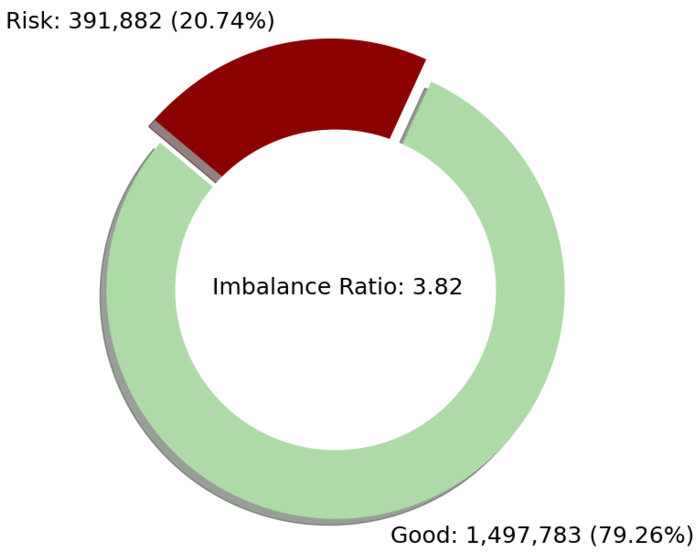
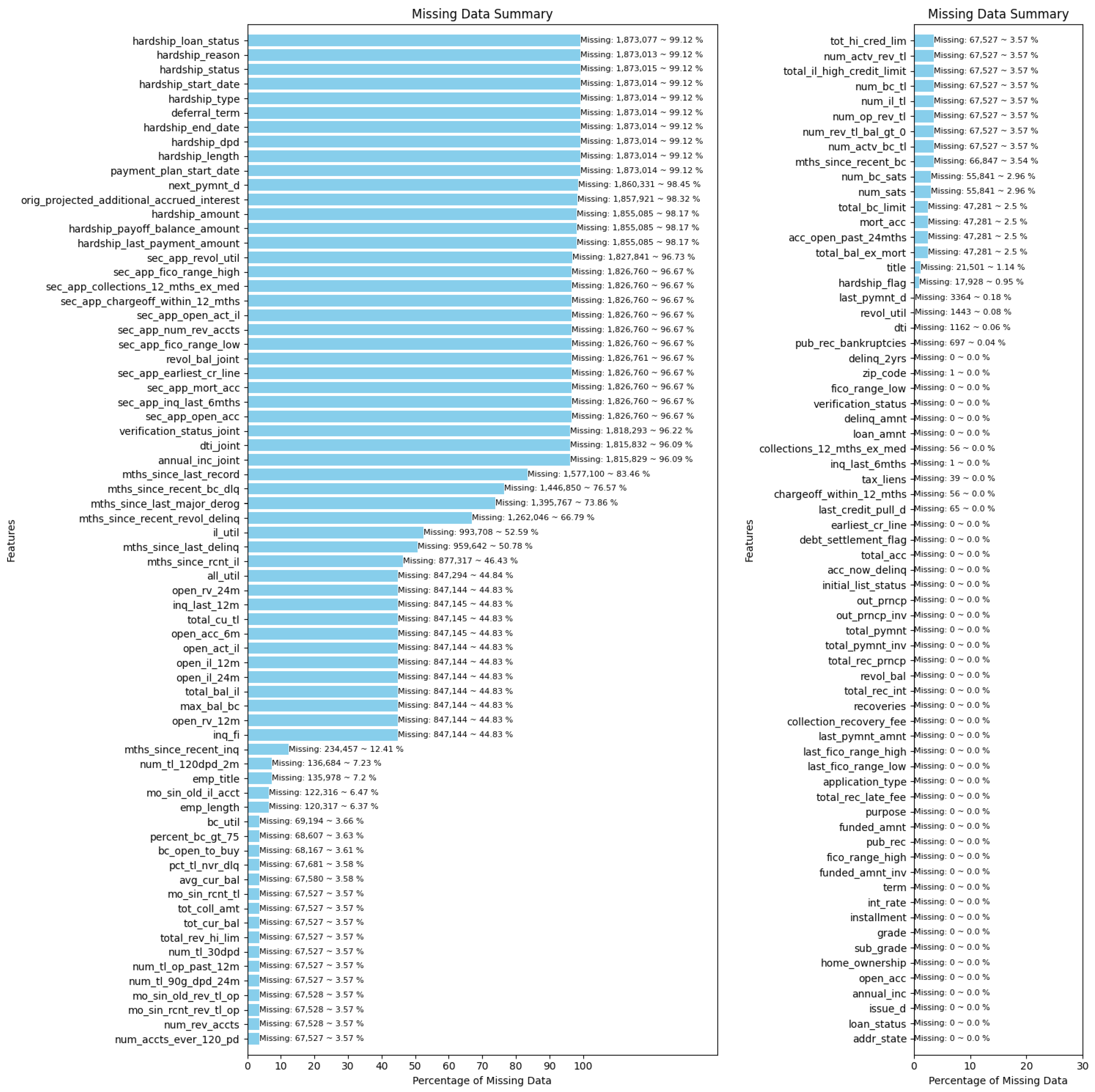
3.1. Data Description and Preprocessing

In this work, financial data provided by the LendingClub Company from 2007 to 2020Q3 [41] were used. The data consist of 2,925,493 records which are divided into various loan statuses as in Table 2. The loan statuses are categorized as “Good” or “Risk” users. The “Fully Paid” status is categorized as “Good” users, whereas “Charged Off”, “In Grace Period”, “Late (16–30 days)”, “Late (31–120 days)”, and “Default” are grouped as “Risk” users. The “Current” status is not explicitly categorized as “Good” or “Risk” since it represents the current state of ongoing payments. “Issued” is also not classified as it may refer to loans that are approved but not yet active. “Does not meet the credit policy” users were excluded in this study. For the experiment, the data contain 1,497,783 samples labeled as “Good” and 391,882 samples labeled as “Risk”, totaling 1,889,665 samples. This is a two-class dataset with an imbalance ratio (IR) equal to 3.82, which shows a slight class imbalance, as displayed in Figure 1. IR is the majority class size divided by the minority class size. A high IR value may affect model performance in some machine learning algorithms, i.e., the majority class is more correctly predicted than the minority class due to imbalanced training data causing model bias. However, the selected algorithms used in this paper like random forest and gradient boosting are quite robust for mild class imbalance. It is more helpful to solve imbalanced data before model training because of the increasing chance of model performance improvement. In addition, the imbalanced data handing methods used in this work are explained in Section 2.3.
There are 141 attributes in the original data which contain many missing values, as illustrated in Figure 2, with high percentages. Some columns need to be dropped and transformed before training the models. The data were preprocessed through the following steps.
(1)
Drop column “id” because it typically serves as a unique identifier for each row, and including it as a feature could lead the model to incorrectly learn patterns that are specific to certain ids rather than generalizing well to new data.
(2)
Drop “url” because it might not provide meaningful information for your model, or its content might be better represented in a different format.
(3)
Drop columns “pymnt_plan” and “policy_code” because every record in the “pymnt_plan” column has the value “n” and every record in the “policy_code” column has the value 1. These columns contain constant values, resulting in the model being unable to differentiate between different data inputs.
(4)
Drop columns that have missing values exceeding 50%. The selected dataset now comprises 101 columns, including 100 features and the loan status.
(5)
In the “int_rate” and “revol_util” columns, convert the percentage values from string format to float.
(6)
For categorical data, fill the missing values with the mode and transform them into numerical values.
(7)
For real value data, fill the missing values with the mean of the existing values.
Now, the dataset comprises 100 features. Each feature was explored in the relationship with its target variable (class label) to rank the importance of features. Mutual information ( M I ) can identify informative features on both linear and non-linear relationships between features and target variables. In feature selection, a feature with a higher mutual information value is considered as more important and typically selected into a training feature set. The importance of these features can be represented by mutual information, as defined in Equation (7).
M I ( X ; Y ) = x X y Y p ( x , y ) · log 2 p ( x , y ) p ( x ) p ( y )
where p ( y ) , p ( x , y ) , and p ( x ) represent the probabilities associated with the target variable Y and the joint and marginal distributions of features X and Y, respectively. The mutual information values for all features are presented in Figure 3. These were used to investigate the impact of feature selection on the performance of the models. The correlation matrix for the first 25 features with the highest mutual information and the class label is depicted in Figure 4. Each cell in the table shows the correlation between two variables. It is often used to understand the relationships between different variables in a dataset. The values range from −1 to 1, where −1 indicates a perfect negative correlation, 1 indicates a perfect positive correlation, and 0 indicates no correlation.

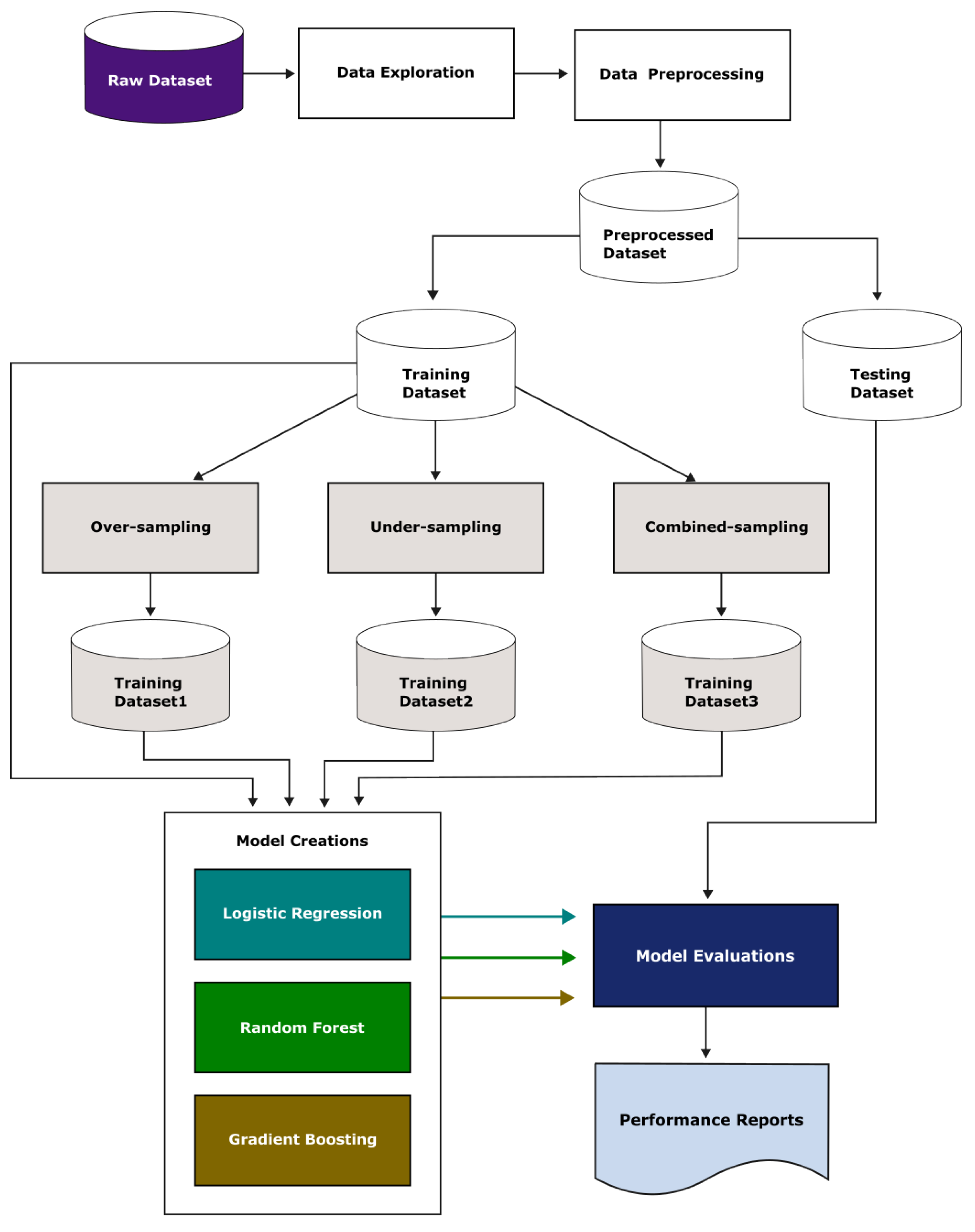
3.2. Model Creations and Evaluations

An overview of the processes in this work is depicted in Figure 5. The raw dataset was explored for characteristics such as data types and missing values. Subsequently, the data were preprocessed to handle missing values. The dataset was then separated into training and testing sets. Two data splitting protocols were experimented with, i.e., hold-out cross-validation with a 70:30 ratio of training and testing sets and 4-fold cross-validation. Next, the training data were prepared in four versions based on imbalanced data handling methods, including original (no sampling), over-sampling, under-sampling, and combined sampling training data. Each training dataset version was used to create three models using logistic regression, random forest, and gradient boosting approaches. The testing dataset was employed to evaluate model performance by calculating A c c u r a c y , P r e c i s i o n , R e c a l l , F 1 s c o r e , and Matthews Correlation Coefficient ( M C C ). In the context of imbalanced data, where one class may dominate the others, using macro-averaging for P r e c i s i o n , R e c a l l , F 1 s c o r e , and M C C can provide a more balanced evaluation across different classes. Then, the confusion matrix was displayed, which is a tabular representation commonly employed to assess the effectiveness of a classification algorithm. This matrix provides a concise overview of the model’s performance by detailing the distribution of predicted and actual class labels (Figure 6). Denote that green and red cells stand for the number of correctly predicted and wrongly predicted samples, respectively. T P and T N are the sample numbers of correctly classified to positive and negative classes, respectively, while F P and F N are the sample numbers of wrongly classified to positive and negative classes, respectively. Subsequently, key performance metrics such as A c c u r a c y , P r e c i s i o n , R e c a l l , F 1 s c o r e , and M C C were computed as follows:
A c c u r a c y is a fundamental metric that measures the overall correctness of a classification model by assessing the proportion of testing data that are correctly predicted out of the total testing data size.
A c c u r a c y = T P + T N T P + T N + F P + F N
P r e c i s i o n (Macro-Averaged) is a metric used to evaluate the P r e c i s i o n of a classification model when dealing with imbalanced datasets. In the context of macro-averaging, P r e c i s i o n is calculated individually for each class and then averaged across all classes.
P r e c i s i o n = 1 C i = 1 C T P i T P i + F P i
where C is the number of classes and T P i and F P i are the true positives and false positives for class i.
R e c a l l (Macro-Averaged) is a metric used to evaluate the R e c a l l of a classification model in the context of imbalanced datasets. In macro averaging, R e c a l l is calculated individually for each class and then averaged across all classes.
R e c a l l = 1 C i = 1 C T P i T P i + F N i
where F N i represents the false negatives for class i.
F 1 s c o r e (Macro-Averaged) is a metric that combines both P r e c i s i o n and R e c a l l , offering a balanced assessment of a model’s performance on imbalanced datasets. In macro averaging, the F 1 S c o r e is calculated individually for each class and then averaged across all classes.
F 1 s c o r e = 1 C i = 1 C 2 × P r e c i s i o n i × R e c a l l i P r e c i s i o n i + R e c a l l i
where P r e c i s i o n i and R e c a l l i are the P r e c i s i o n and R e c a l l for class i.
The Matthews Correlation Coefficient ( M C C ) is one of the metrics suitable for evaluating binary classification models, especially models that were trained by imbalanced datasets, because true positives ( T P ), true negatives ( T N ), false positives ( F P ), and false negatives ( F N ) are all taken into account in its formula. The M C C is defined as:
M C C = ( T P × T N ) ( F P × F N ) ( T P + F P ) ( T P + F N ) ( T N + F P ) ( T N + F N ) .
The M C C value ranges between −1 and 1. The best and worst M C C values are 1 and −1, respectively. When the M C C value is 0, this means that the model performance is not greater than that of random guessing.

4. Results and Discussion

To solve an imbalanced data issue, four versions of training datasets, including data with no sampling, over-sampling, under-sampling, and combined sampling, were experimented with. The number of data samples in each training dataset is illustrated in Figure 7. Experiments with two methods of training and testing data splitting, 70:30 hold-out cross-validation and 4-fold cross-validation, were performed.

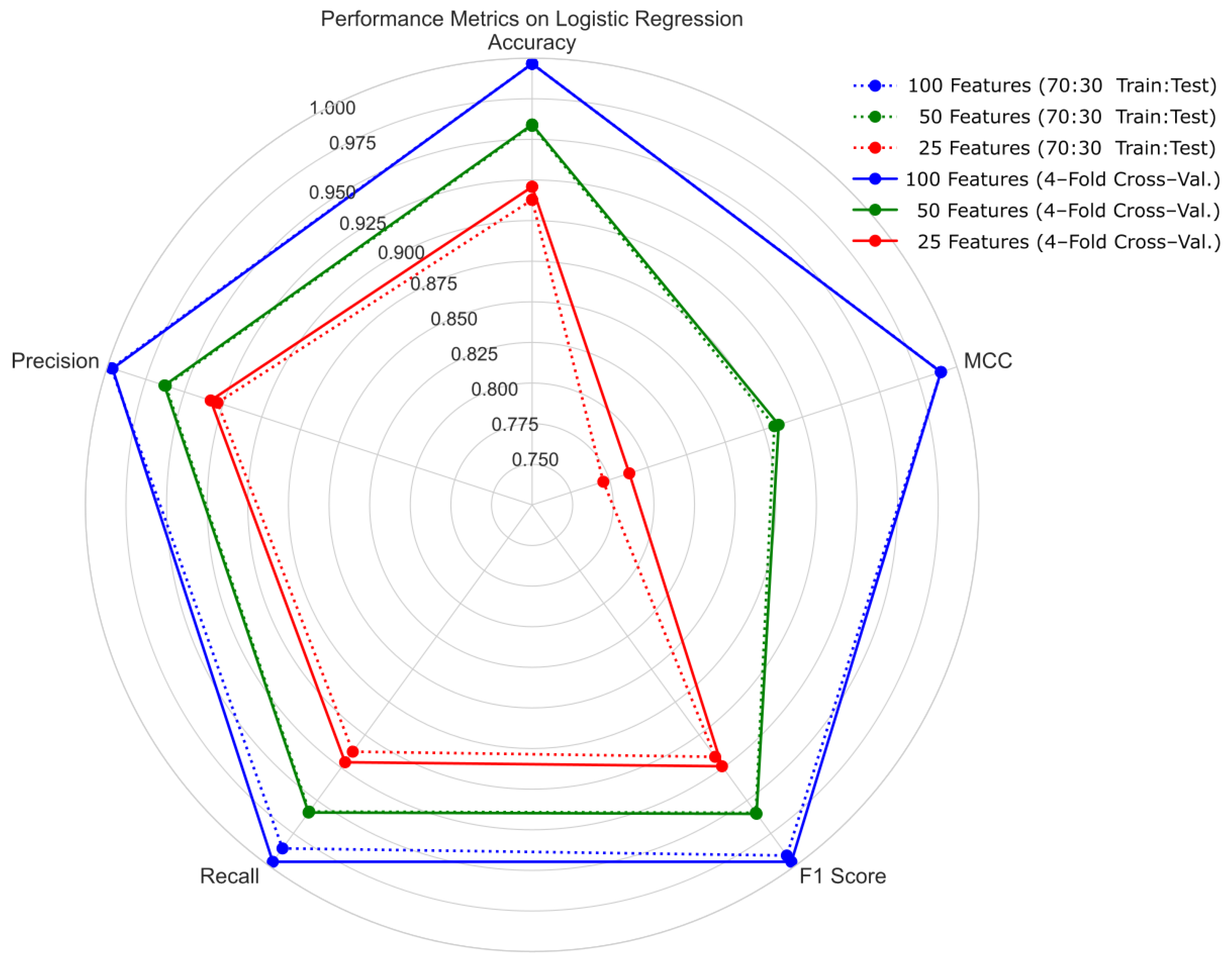
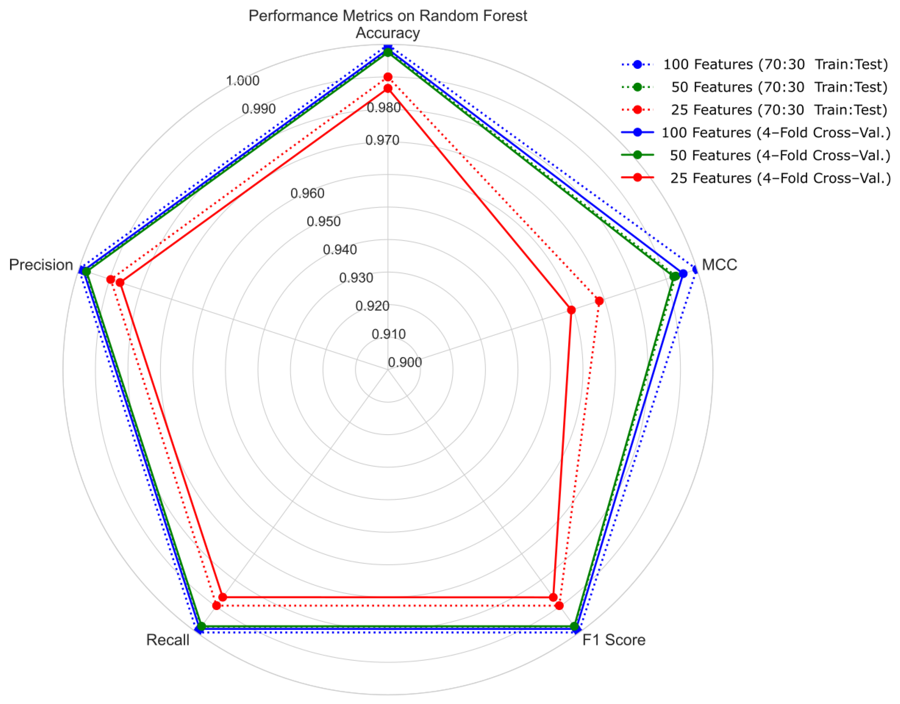
4.1. Hold-Out Cross-Validation with 70:30 Ratio of Training and Testing Sets

The confusion matrices of testing data prediction were yielded by logistic regression, random forest, and gradient boosting models, which were trained by four versions of training data as shown in Figure 8a–d. The five performance metrics, i.e., A c c u r a c y , P r e c i s i o n , R e c a l l , F 1 s c o r e , and M C C , are shown in Table 3. The comparably highest effective performance, i.e., the first and second ranks across the five metrics, was yielded by the random forest model as well as the gradient boosting model trained by data with over-sampling. In detail, the gradient boosting model with the over-sampling technique showed slightly better results, i.e., performance values were 1 for all five measures, but this hold-out cross-validation experiment was performed one time due to convenience for a very large dataset, at first. Therefore, for a solid experimental conclusion, another 4-fold cross-validation experiment was also studied.

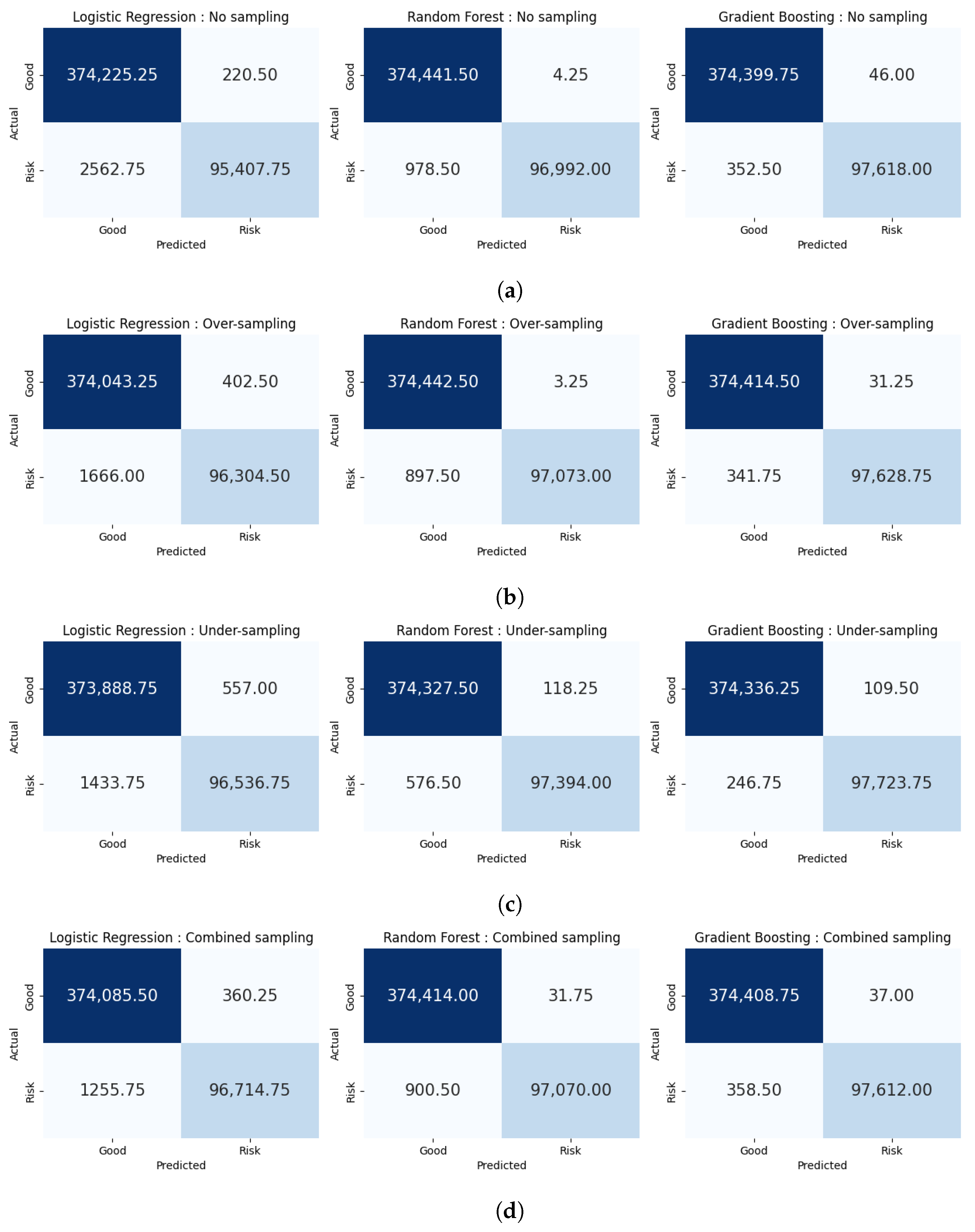
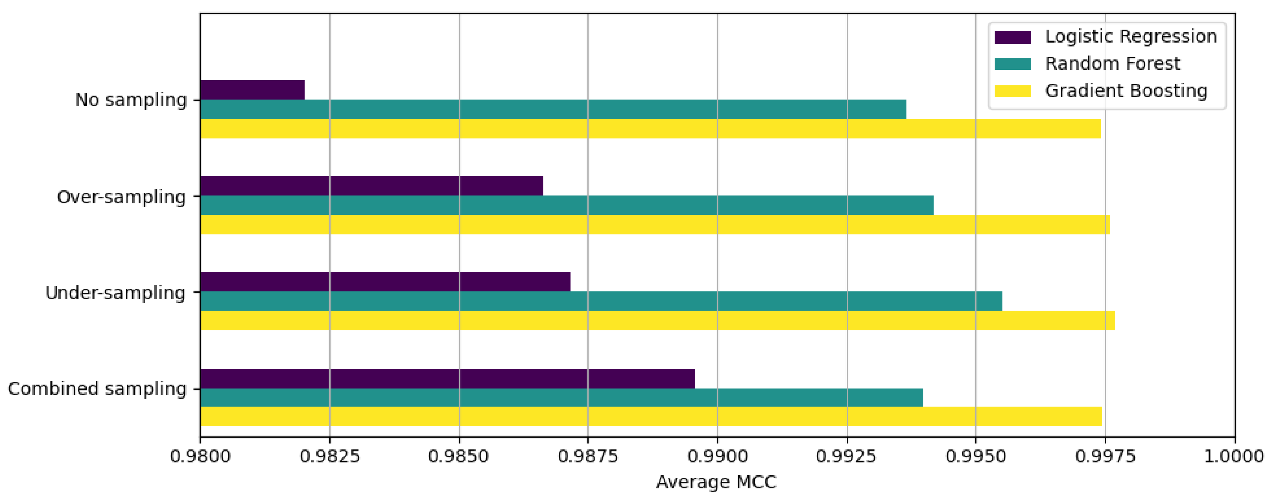
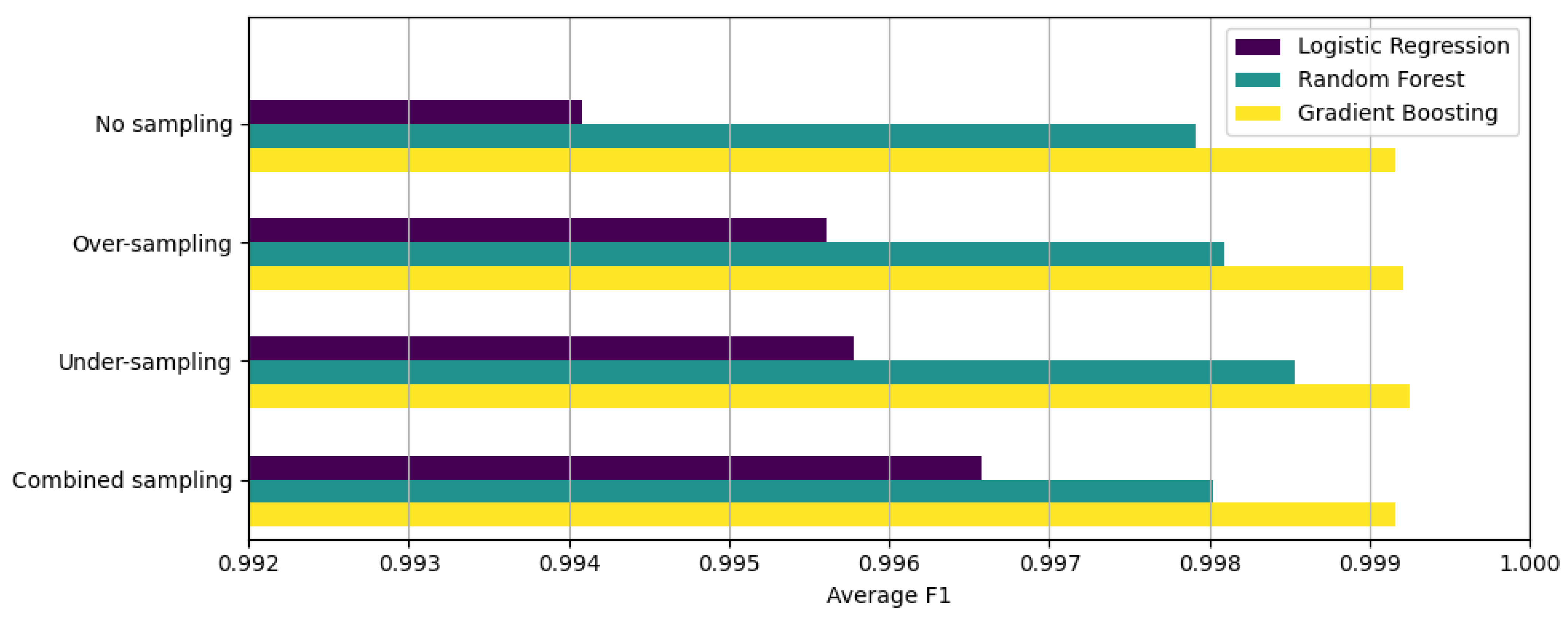
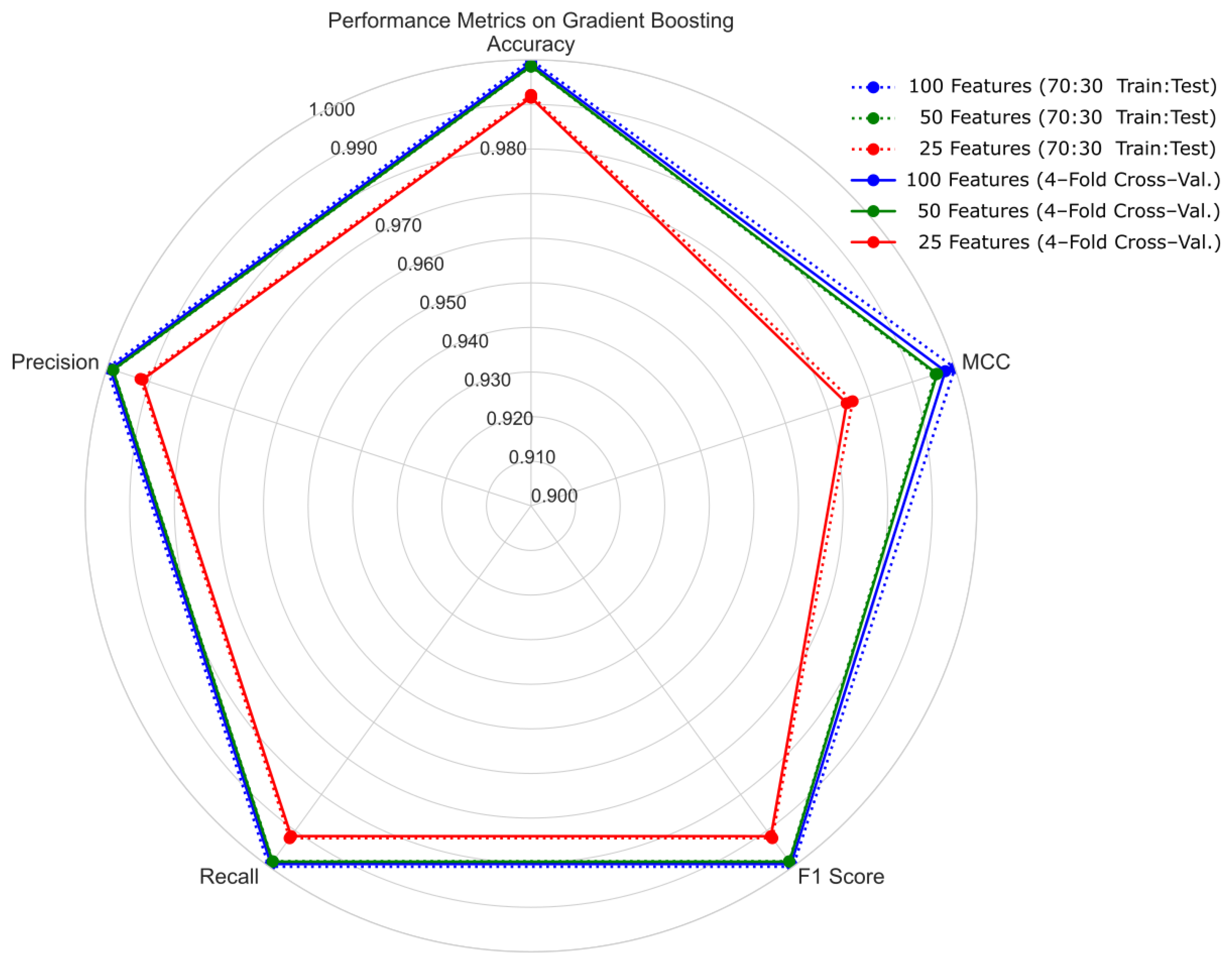
4.2. Four-Fold Cross-Validation

The average confusion matrices for 4-fold cross-validation results are illustrated in Figure 9a–d. The performance metrics for logistic regression, random forest, and gradient boosting are shown in Table 4, Table 5, and Table 6, respectively. Three imbalanced data handling approaches, including over-sampling, under-sampling, and combined sampling, can improve the performance of models trained by logistic regression, random forest, and gradient boosting algorithms. Considering only the performance of logistic regression models, models with the combined sampling approach outperform the others. For random forest and gradient boosting models, when the under-sampling approach was employed, they both showed better model performance compared to the other sampling approaches. In general, from all 4-fold cross-validation results, gradient boosting models with the under-sampling method gave the superior performance. The additionally depicted comparisons of M C C and F 1 s c o r e are shown in Figure 10 and Figure 11, respectively.
Overall result summation from both experiments of the two cross-validation methods indicates that the gradient boosting algorithm with an appropriate data solving technique for supervised model training offers the very impressive ability of resulting in models that correctly classify both “Good” and “Risk” instances.
Next, the feature selection method was applied, i.e., computing and ranking the mutual information ( M I ) values of each feature, in order to reasonably select important features of the smaller feature size k of the training set. So, the training data with the best imbalanced data handling technique for each model were further explored by preparing a smaller number of k features via their M I values to assess the trade-offs between the different important feature sizes and their impact on model performance. The features were ranked based on their computed values of mutual information. Three numbers of feature size, i.e., k = 25, 50, and 100, were experimented with. The results of logistic regression, random forest, and gradient boosting models on both 70:30 hold-out cross-validation and 4-fold cross-validation with three different feature sizes are shown in Figure 12, Figure 13, and Figure 14, respectively. Generally, the performance of all three supervised models was reduced slightly. For k = 25 and 50 important features as training data, gradient boosting models showed better results than logistic regression and random forest models. Focusing on k = 50 important features, random forest and gradient boosting models yielded five performance values, i.e., A c c u r a c y , P r e c i s i o n , R e c a l l , F 1 s c o r e , and M C C , greater than 99%, whereas logistic regression models gave four performance values, excepting M C C , higher than 95%. For k = 25 important features, gradient boosting models still yielded A c c u r a c y , P r e c i s i o n , R e c a l l , and F 1 s c o r e values not less than 99%, but M C C values reduced to around 97.5%. These show that when the number of features was reduced by half ( k = 50), the performance values were reduced by only less than 1%. Although the number of features was approximately reduced by 75% ( k = 25), the performance values were reduced by only less than 1–2%. Apart from that, the performance of gradient boosting models using k = 100 important features was better than that of the others on both 70:30 hold-out cross-validation and 4-fold cross-validation experiments.
In order to additionally display our results compared with previous research, the performance comparison of the proposed methods with other existing works on various versions of LendingClub data is shown in Figure 15. Based on A c c u r a c y , the proposed methods outperform the others.

5. Conclusions and Future Work

This study provided a very efficient solution to the problem of credit risk prediction. To investigate the improved predictive model results that could be better than those from previous works, three popular machine learning methods, including logistic regression, random forest, and gradient boosting, were employed. Additionally, the imbalanced data problem was resolved by experimenting with various sampling strategies: under-sampling, over-sampling, and combined sampling. Based on our best model performance outcomes, the over-sampling as well as under-sampling methods robustly manage class-imbalanced data, especially when the training model uses the gradient boosting method. In addition, the feature numbers of the data were reduced by selecting only important features for the training set according to their ranks computed by mutual information. Another experiment was performed using two reduced feature sets, the half size as well as the one-fourth size of its original feature size. The resulting model performance was just barely decreased. Remarkably, both random forest and gradient boosting models created by the reduced feature sets with the half size showed impressive Accuracy values, higher than 99%.
This comprehensive analysis enhances better understanding of credit risk prediction using a supervised learning method combined with various imbalanced data solving strategies. Furthermore, the importance of features based on mutual information was addressed in order to increase model performance with the smaller feature size of training data. Our proposed method and results offer a simple way to select important features with the reduced size by ranking the mutual information values of each feature. In spite of this method not providing the most optimal size with the best performance, it can apply to other large credit risk data with different feature sets. This approach does not significantly decrease performance, but there might be better methods available. In future work, it may be beneficial to further investigate parameter optimization, particularly in handling imbalanced data, and explore alternative feature selection methods beyond mutual information, such as correlation and symmetrical uncertainty, to improve model performance. In addition, ensemble techniques could offer performance improvement of those small feature sizes. Apart from that, real-time data streams and dynamic model updating may increase the adaptability of credit risk prediction systems.

Author Contributions

Conceptualization, N.W. and S.T.; methodology, N.W. and S.T.; validation, N.W. and S.T.; formal analysis, N.W. and P.W.; investigation, N.W., P.W. and S.T.; data curation, N.W. and P.W.; writing—original draft preparation, N.W. and S.T.; writing—review and editing, N.W., S.J., S.S. and S.T.; visualization, N.W., P.W. and S.T.; supervision, S.J. and S.S. All authors have read and agreed to the published version of the manuscript.

Funding

This research received no external funding.

Institutional Review Board Statement

Not applicable.

Informed Consent Statement

Not applicable.

Data Availability Statement

The used data are publicly available at https://www.kaggle.com/datasets/ethon0426/lending-club-20072020q1 (accessed on 17 January 2024).

Conflicts of Interest

The authors declare no conflicts of interest.

References

  1. Noriega, J.P.; Rivera, L.A.; Herrera, J.A. Machine Learning for Credit Risk Prediction: A Systematic Literature Review. Data 2023, 8, 169. [Google Scholar] [CrossRef]
  2. Gjeçi, A.; Marinč, M.; Rant, V. Non-performing loans and bank lending behaviour. Risk Manag. 2023, 25, 7. [Google Scholar] [CrossRef]
  3. Liu, H.; Qiao, H.; Wang, S.; Li, Y. Platform Competition in Peer-to-Peer Lending Considering Risk Control Ability. Eur. J. Oper. Res. 2019, 274, 280–290. [Google Scholar] [CrossRef]
  4. Sulastri, R.; Janssen, M. Challenges in Designing an Inclusive Peer-to-Peer (P2P) Lending System. In Proceedings of the 24th Annual International Conference on Digital Government Research, DGO ‘23, New York, NY, USA, 11–14 July 2023; pp. 55–65. [Google Scholar] [CrossRef]
  5. Ko, P.C.; Lin, P.C.; Do, H.T.; Huang, Y.F. P2P Lending Default Prediction Based on AI and Statistical Models. Entropy 2022, 24, 801. [Google Scholar] [CrossRef]
  6. Kurniawan, R. Examination of the Factors Contributing To Financial Technology Adoption in Indonesia using Technology Acceptance Model: Case Study of Peer to Peer Lending Service Platform. In Proceedings of the 2019 International Conference on Information Management and Technology (ICIMTech), Denpasar, Indonesia, 19–20 August 2019; Volume 1, pp. 432–437. [Google Scholar] [CrossRef]
  7. Wang, Q.; Xiong, X.; Zheng, Z. Platform Characteristics and Online Peer-to-Peer Lending: Evidence from China. Financ. Res. Lett. 2021, 38, 101511. [Google Scholar] [CrossRef]
  8. Ma, Z.; Hou, W.; Zhang, D. A credit risk assessment model of borrowers in P2P lending based on BP neural network. PLoS ONE 2021, 16, e0255216. [Google Scholar] [CrossRef]
  9. Moscato, V.; Picariello, A.; Sperlí, G. A benchmark of machine learning approaches for credit score prediction. Expert Syst. Appl. 2021, 165, 113986. [Google Scholar] [CrossRef]
  10. Liu, W.; Fan, H.; Xia, M. Credit scoring based on tree-enhanced gradient boosting decision trees. Expert Syst. Appl. 2022, 189, 116034. [Google Scholar] [CrossRef]
  11. Kriebel, J.; Stitz, L. Credit default prediction from user-generated text in peer-to-peer lending using deep learning. Eur. J. Oper. Res. 2022, 302, 309–323. [Google Scholar] [CrossRef]
  12. Uddin, N.; Uddin Ahamed, M.K.; Uddin, M.A.; Islam, M.M.; Talukder, M.A.; Aryal, S. An ensemble machine learning based bank loan approval predictions system with a smart application. Int. J. Cogn. Comput. Eng. 2023, 4, 327–339. [Google Scholar] [CrossRef]
  13. Yin, W.; Kirkulak-Uludag, B.; Zhu, D.; Zhou, Z. Stacking ensemble method for personal credit risk assessment in Peer-to-Peer lending. Appl. Soft Comput. 2023, 142, 110302. [Google Scholar] [CrossRef]
  14. Muslim, M.A.; Nikmah, T.L.; Pertiwi, D.A.A.; Dasril, Y. New model combination meta-learner to improve accuracy prediction P2P lending with stacking ensemble learning. Intell. Syst. Appl. 2023, 18, 200204. [Google Scholar] [CrossRef]
  15. Niu, K.; Zhang, Z.; Liu, Y.; Li, R. Resampling ensemble model based on data distribution for imbalanced credit risk evaluation in P2P lending. Inf. Sci. 2020, 536, 120–134. [Google Scholar] [CrossRef]
  16. Li, X.; Ergu, D.; Zhang, D.; Qiu, D.; Cai, Y.; Ma, B. Prediction of loan default based on multi-model fusion. Procedia Comput. Sci. 2022, 199, 757–764. [Google Scholar] [CrossRef]
  17. He, H.; Bai, Y.; Garcia, E.A.; Li, S. ADASYN: Adaptive synthetic sampling approach for imbalanced learning. In Proceedings of the 2008 IEEE International Joint Conference on Neural Networks (IEEE World Congress on Computational Intelligence), Hong Kong, 1–6 June 2008; pp. 1322–1328. [Google Scholar] [CrossRef]
  18. Chen, Y.R.; Leu, J.S.; Huang, S.A.; Wang, J.T.; Takada, J.I. Predicting Default Risk on Peer-to-Peer Lending Imbalanced Datasets. IEEE Access 2021, 9, 73103–73109. [Google Scholar] [CrossRef]
  19. Kumar, V.L.; Natarajan, S.; Keerthana, S.; Chinmayi, K.M.; Lakshmi, N. Credit Risk Analysis in Peer-to-Peer Lending System. In Proceedings of the 2016 IEEE International Conference on Knowledge Engineering and Applications (ICKEA), Singapore, 28–30 September 2016; pp. 193–196. [Google Scholar] [CrossRef]
  20. Setiawan, N. A Comparison of Prediction Methods for Credit Default on Peer to Peer Lending using Machine Learning. Procedia Comput. Sci. 2019, 157, 38–45. [Google Scholar] [CrossRef]
  21. Liu, Z.; Zhang, Z.; Yang, H.; Wang, G.; Xu, Z. An innovative model fusion algorithm to improve the recall rate of peer-to-peer lending default customers. Intell. Syst. Appl. 2023, 20, 200272. [Google Scholar] [CrossRef]
  22. Ziemba, P.; Becker, J.; Becker, A.; Radomska-Zalas, A.; Pawluk, M.; Wierzba, D. Credit Decision Support Based on Real Set of Cash Loans Using Integrated Machine Learning Algorithms. Electronics 2021, 10, 2099. [Google Scholar] [CrossRef]
  23. Dong, H.; Liu, R.; Tham, A.W. Accuracy Comparison between Five Machine Learning Algorithms for Financial Risk Evaluation. J. Risk Financ. Manag. 2024, 17, 50. [Google Scholar] [CrossRef]
  24. Stoltzfus, J.C. Logistic regression: A brief primer. Acad. Emerg. Med. 2011, 18, 1099–1104. [Google Scholar] [CrossRef]
  25. Manglani, R.; Bokhare, A. Logistic Regression Model for Loan Prediction: A Machine Learning Approach. In Proceedings of the 2021 Emerging Trends in Industry 4.0 (ETI 4.0), Raigarh, India, 19–21 May 2021; pp. 1–6. [Google Scholar] [CrossRef]
  26. Kadam, E.; Gupta, A.; Jagtap, S.; Dubey, I.; Tawde, G. Loan Approval Prediction System using Logistic Regression and CIBIL Score. In Proceedings of the 2023 4th International Conference on Electronics and Sustainable Communication Systems (ICESC), Coimbatore, India, 7–9 August 2023; pp. 1317–1321. [Google Scholar] [CrossRef]
  27. Zhu, X.; Chu, Q.; Song, X.; Hu, P.; Peng, L. Explainable prediction of loan default based on machine learning models. Data Sci. Manag. 2023, 6, 123–133. [Google Scholar] [CrossRef]
  28. Lin, M.; Chen, J. Research on Credit Big Data Algorithm Based on Logistic Regression. Procedia Comput. Sci. 2023, 228, 511–518. [Google Scholar] [CrossRef]
  29. Breiman, L. Random forests. Mach. Learn. 2001, 45, 5–32. [Google Scholar] [CrossRef]
  30. Zhu, L.; Qiu, D.; Ergu, D.; Ying, C.; Liu, K. A study on predicting loan default based on the random forest algorithm. Procedia Comput. Sci. 2019, 162, 503–513. [Google Scholar] [CrossRef]
  31. Rao, C.; Liu, M.; Goh, M.; Wen, J. 2-stage modified random forest model for credit risk assessment of P2P network lending to “Three Rurals” borrowers. Appl. Soft Comput. 2020, 95, 106570. [Google Scholar] [CrossRef]
  32. Reddy, C.S.; Siddiq, A.S.; Jayapandian, N. Machine Learning based Loan Eligibility Prediction using Random Forest Model. In Proceedings of the 2022 7th International Conference on Communication and Electronics Systems (ICCES), Coimbatore, India, 12–14 November 2022; pp. 1073–1079. [Google Scholar] [CrossRef]
  33. Friedman, J.H. Greedy function approximation: A gradient boosting machine. Ann. Stat. 2001, 29, 1189–1232. [Google Scholar] [CrossRef]
  34. Zhou, L.; Fujita, H.; Ding, H.; Ma, R. Credit risk modeling on data with two timestamps in peer-to-peer lending by gradient boosting. Appl. Soft Comput. 2021, 110, 107672. [Google Scholar] [CrossRef]
  35. Zhu, X.; Chen, J. Risk Prediction of P2P Credit Loans Overdue Based on Gradient Boosting Machine Model. In Proceedings of the 2021 IEEE International Conference on Power, Intelligent Computing and Systems (ICPICS), Shenyang, China, 29–31 July 2021; pp. 212–216. [Google Scholar] [CrossRef]
  36. Miaojun Bai, Y.Z.; Shen, Y. Gradient boosting survival tree with applications in credit scoring. J. Oper. Res. Soc. 2022, 73, 39–55. [Google Scholar] [CrossRef]
  37. Qian, H.; Wang, B.; Yuan, M.; Gao, S.; Song, Y. Financial distress prediction using a corrected feature selection measure and gradient boosted decision tree. Expert Syst. Appl. 2022, 190, 116202. [Google Scholar] [CrossRef]
  38. Chawla, N.V.; Bowyer, K.W.; Hall, L.O.; Kegelmeyer, W.P. SMOTE: Synthetic Minority over-Sampling Technique. J. Artif. Int. Res. 2002, 16, 321–357. [Google Scholar] [CrossRef]
  39. Bach, M.; Werner, A.; Palt, M. The Proposal of Undersampling Method for Learning from Imbalanced Datasets. Procedia Comput. Sci. 2019, 159, 125–134. [Google Scholar] [CrossRef]
  40. Batista, G.E.A.P.A.; Prati, R.C.; Monard, M.C. A Study of the Behavior of Several Methods for Balancing Machine Learning Training Data. SIGKDD Explor. Newsl. 2004, 6, 20–29. [Google Scholar] [CrossRef]
  41. Ethon0426. Lending Club 2007–2020Q3. Available online: https://www.kaggle.com/datasets/ethon0426/lending-club-20072020q1 (accessed on 17 January 2024).
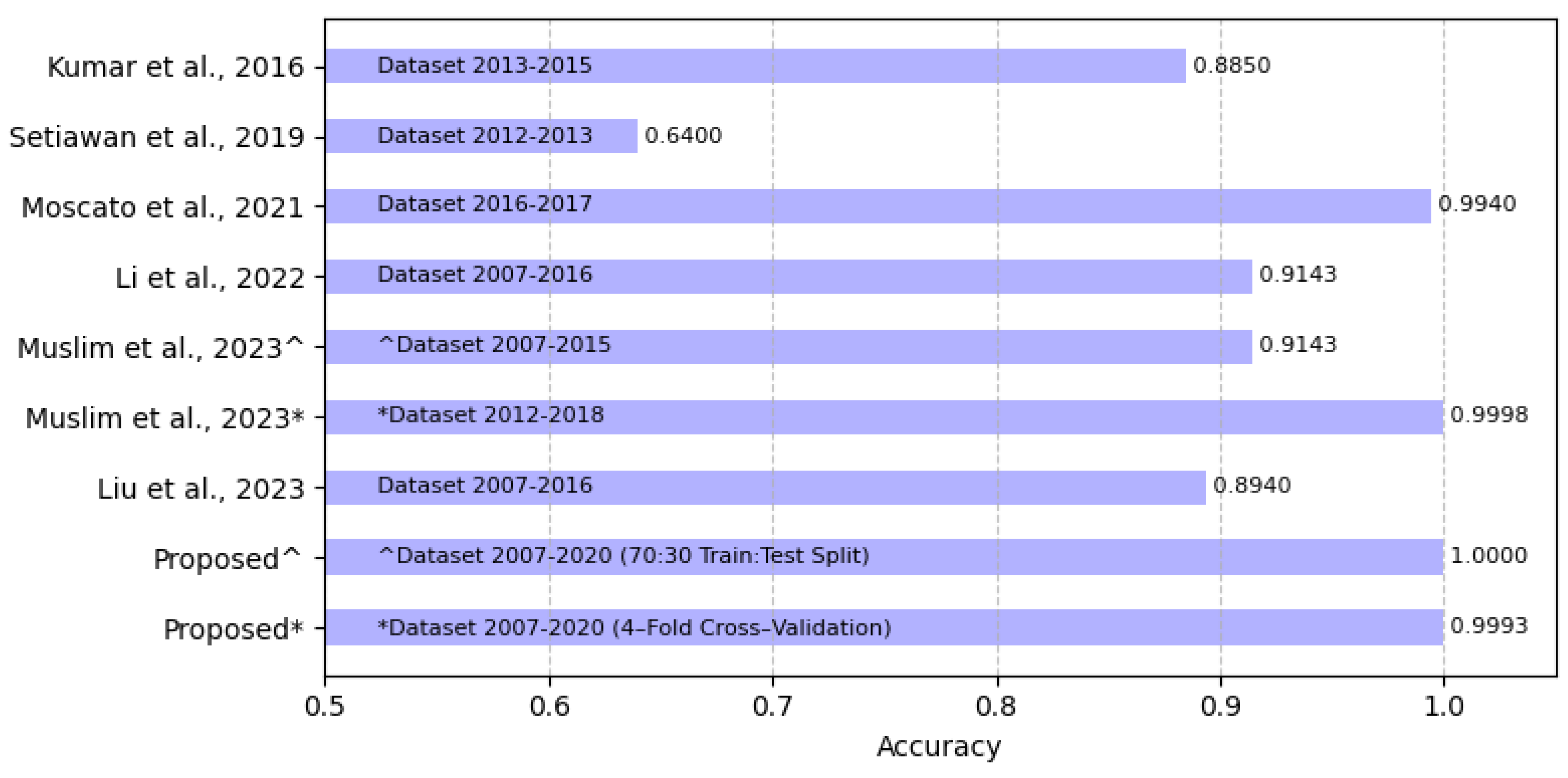
Figure 1. Class imbalance of our experimental dataset from LendingClub dataset.
Bdcc 08 00028 g001
Figure 2. The summary of missing values on each attribute excluding the “id”, “url”, “pymnt_plan”, and “policy_code” attributes.
Bdcc 08 00028 g002
Figure 3. A summary of mutual information ( M I ) across the 100 features used.
Bdcc 08 00028 g003
Figure 4. Correlation matrix on the first 25 highest mutual information features.
Bdcc 08 00028 g004
Figure 5. Overview of proposed methodology.
Bdcc 08 00028 g005
Figure 6. Two-by-two confusion matrix.
Bdcc 08 00028 g006
Figure 7. Comparison of training data sizes on various sampling methods.
Bdcc 08 00028 g007
Figure 8. Confusion matrices of 70:30 hold-out cross-validation results. (a) No sampling testing data (original data). (b) Over-sampling testing data. (c) Under-sampling testing data. (d) Combined sampling testing data.
Bdcc 08 00028 g008
Figure 9. Average confusion matrices of four-fold cross-validation results. (a) No sampling testing data (original data). (b) Over-sampling testing data. (c) Under-sampling testing data. (d) Combined sampling testing data.
Bdcc 08 00028 g009
Figure 10. Average M C C comparison for different sampling methods.
Bdcc 08 00028 g010
Figure 11. Average F 1 s c o r e comparison for different sampling methods.
Bdcc 08 00028 g011
Figure 12. Logistic regression model performance on five metrics for k different numbers of features, i.e., k = 25, 50, and 100.
Bdcc 08 00028 g012
Figure 13. Random forest model performance on five metrics for k different numbers of features, i.e., k = 25, 50, and 100.
Bdcc 08 00028 g013
Figure 14. Gradient boosting model performance on five metrics for k different numbers of features, i.e., k = 25, 50, and 100.
Bdcc 08 00028 g014
Figure 15. A c c u r a c y of the proposed method compared with existing works on various versions of LendingClub data. Denote that ^ and * symbols stand for the different dataset or experiment in the same work.
Bdcc 08 00028 g015
Table 1. Research paper examples of various versions of LendingClub data.
ResearchLendingClub DataImbalance SolvingMLBest Performance
[19]Year: 2013–2015-Random forest A c c u r a c y : 0.885
Samples: 656,724 Decision tree
Features: 115 Bagging
Classes: 2 ({good}; {bad})
[20]Year: 2012–2013-BPSOSVM + A c c u r a c y : 0.64
Samples: 164,620 Extremely randomized tree P r e c i s i o n : 062
Features: 34 R e c a l l : 0.65
Classes: 2 ({Charged Off, F 1 s c o r e : 0.61
Late (31–120 days),
Default}; {Fully Paid})
[9]Year: 2016–2017Under-samplingLogistic regression A c c u r a c y : 0.64
Samples: 877,956Over-samplingRandom forest A U C : 0.71
Features: 151HybridMLP T P R : 0.66
Classes: 2 ({Fully Paid}; T N R : 0.64
{Charged Off})
[16]Year: 2019ADASYNFusion model A c c u r a c y : 0.994
Samples: 128,262 (logistic regression, R e c a l l : 0.99
Features: 150 random forest, F 1 s c o r e : 0.99
Classes: no details and CatBoost)
[14]Year: 2007–2015SMOTELGBFS A c c u r a c y : 0.9143
Samples: 9578 + StackingXGBoos R e c a l l : 0.9151
Features: 14 F 1 s c o r e : 0.9165
Classes: 2 ({not.fully.paid};
{fully.paid})
[14]Year: 2012–2018SMOTELGBFS A c c u r a c y : 0.99982
Samples: 2,875,146 + StackingXGBoos R e c a l l : 0.9999
Features: 18 F 1 s c o r e : 0.9999
Classes: 2
loan_status { 0 , 1 }
[21]Year: 2007–2016SMOTELGB-XGB-Stacking A c c u r a c y : 0.8940
Samples: 396, 030 R e c a l l : 0.7131
Features: 27 A U C : 0.7975
Classes: 2 ({Fully Paid};
{Charged Off})
Table 2. Dataset from LendingClub company from 2007 to 2020Q3 and loan status distribution.
Loan StatusCountLabel
“Fully Paid”1,497,783“Good”
“Charged Off”362,548“Risk”
“In Grace Period”10,028“Risk”
“Late (16–30 days)”2719“Risk”
“Late (31–120 days)”16,154“Risk”
“Default”433“Risk”
“Current”1,031,016-
“Issued”2062-
“Does not meet the credit policy. Status: Fully Paid”1988-
“Does not meet the credit policy. Status: Charged Off”761-
Total2,925,493
Table 3. The performance of three different machine learning techniques with various sampling approaches in the 70:30 hold-out cross-validation experiment. The superscript numbers in the brackets denote the performance ranking based on the evaluation measure in each column.
Imbalanced Data Handling TechniqueModelAccuracyPrecisionRecallF1 ScoreMCC
No sampling
(original data)
Logistic regression0.9882   ( 12 ) 0.9920   ( 10 ) 0.9506   ( 12 ) 0.9709   ( 12 ) 0.9639   ( 12 )
Random forest0.9979   ( 4 ) 0.9999   ( 3 ) 0.9902   ( 6 ) 0.9951   ( 4 ) 0.9938   ( 4 )
Gradient boosting0.9961   ( 9 ) 0.9999   ( 3 ) 0.9812   ( 10 ) 0.9905   ( 9 ) 0.9882   ( 9 )
Over-samplingLogistic regression0.9914   ( 11 ) 0.9895   ( 12 ) 0.9685   ( 11 ) 0.9789   ( 11 ) 0.9736   ( 11 )
Random forest0.9999   ( 2 ) 1.0000   ( 1 ) 0.9999   ( 2 ) 0.9999   ( 2 ) 0.9999   ( 2 )
Gradient boosting1.0000   ( 1 ) 1.0000   ( 1 ) 1.0000   ( 1 ) 1.0000   ( 1 ) 1.0000   ( 1 )
Under-samplingLogistic regression0.9950   ( 10 ) 0.9900   ( 11 ) 0.9856   ( 9 ) 0.9878   ( 10 ) 0.9847   ( 10 )
Random forest0.9986   ( 3 ) 0.9989   ( 8 ) 0.9940   ( 3 ) 0.9965   ( 3 ) 0.9956   ( 3 )
Gradient boosting0.9979   ( 4 ) 0.9992   ( 7 ) 0.9908   ( 4 ) 0.9950   ( 5 ) 0.9937   ( 5 )
Combined samplingLogistic regression0.9966   ( 8 ) 0.9973   ( 9 ) 0.9864   ( 8 ) 0.9918   ( 8 ) 0.9897   ( 8 )
Random forest0.9979   ( 4 ) 0.9994   ( 6 ) 0.9907   ( 5 ) 0.9950   ( 5 ) 0.9937   ( 5 )
Gradient boosting0.9972   ( 7 ) 0.9997   ( 5 ) 0.9866   ( 7 ) 0.9931   ( 7 ) 0.9914   ( 7 )
Table 4. Performance metrics for logistic regression with different sampling approaches in 4-fold cross-validation (4-fold cv) experiments.
Method4-Fold cvAccuracyPrecisionRecallF1 ScoreMCC
Logistic regression: No samplingFold 10.9936370.9936600.9936370.9936070.980512
Fold 20.9942830.9943020.9942830.9942580.982578
Fold 30.9939880.9940150.9939880.9939600.981772
Fold 40.9945260.9945460.9945260.9945030.983267
Average0.9941080.9941310.9941080.9940820.982032
Logistic regression: Over-samplingFold 10.9959700.9959720.9959700.9959600.987666
Fold 20.9962020.9962010.9962020.9961960.988435
Fold 30.9953490.9953520.9953490.9953370.985900
Fold 40.9949640.9949640.9949640.9949510.984602
Average0.9956210.9956220.9956210.9956110.986651
Logistic regression: Under-samplingFold 10.9961880.9961850.9961880.9961820.988336
Fold 20.9958380.9958360.9958380.9958310.987324
Fold 30.9951700.9951650.9951700.9951610.985355
Fold 40.9959480.9959450.9959480.9959430.987621
Average0.9957860.9957830.9957860.9957790.987159
Logistic regression: Combined samplingFold 10.9970490.9970500.9970490.9970440.990975
Fold 20.9964180.9964210.9964180.9964110.989094
Fold 30.9968330.9968330.9968330.9968280.990406
Fold 40.9960160.9960120.9960160.9960110.987829
Average0.9965790.9965790.9965790.9965730.989576
Table 5. Performance metrics for random forest with different sampling approaches in 4-fold cross-validation (4-fold cv) experiments.
Method4-Fold cvAccuracyPrecisionRecallF1 ScoreMCC
Random forest: No samplingFold 10.9979930.9979980.9979930.9979900.993868
Fold 20.9979490.9979540.9979490.9979450.993762
Fold 30.9978180.9978230.9978180.9978130.993395
Fold 40.9979190.9979240.9979190.9979150.993651
Average0.9979200.9979250.9979200.9979160.993669
Random forest: Over-samplingFold 10.9981140.9981180.9981140.9981110.994237
Fold 20.9981670.9981710.9981670.9981640.994425
Fold 30.9980500.9980550.9980500.9980470.994100
Fold 40.9980420.9980470.9980420.9980390.994026
Average0.9980930.9980980.9980930.9980900.994197
Random forest: Under-samplingFold 10.9985670.9985680.9985670.9985660.995621
Fold 20.9985480.9985480.9985480.9985470.995583
Fold 30.9984780.9984780.9984780.9984770.995393
Fold 40.9985250.9985250.9985250.9985230.995497
Average0.9985290.9985300.9985290.9985280.995523
Random forest: Combined samplingFold 10.9980760.9980790.9980760.9980730.994120
Fold 20.9979870.9979900.9979870.9979840.993877
Fold 30.9980590.9980630.9980590.9980560.994125
Fold 40.9979850.9979890.9979850.9979810.993851
Average0.9980270.9980300.9980270.9980230.993993
Table 6. Performance metrics for gradient boosting with different sampling approaches in 4-fold cross-validation (4-fold cv) experiments.
Method4-Fold cvAccuracyPrecisionRecallF1 ScoreMCC
Gradient boosting: No samplingFold 10.9991720.9991730.9991720.9991720.997471
Fold 20.9991300.9991300.9991300.9991300.997355
Fold 30.9992170.9992170.9992170.9992160.997630
Fold 40.9991070.9991070.9991070.9991060.997275
Average0.9991560.9991570.9991560.9991560.997433
Gradient boosting: Over-samplingFold 10.9992800.9992810.9992800.9992800.997801
Fold 20.9991790.9991790.9991790.9991780.997503
Fold 30.9992080.9992090.9992080.9992080.997605
Fold 40.9991740.9991750.9991740.9991740.997482
Average0.9992100.9992110.9992100.9992100.997598
Gradient boosting: Under-samplingFold 10.9992850.9992840.9992850.9992840.997814
Fold 20.9992760.9992760.9992760.9992760.997799
Fold 30.9992570.9992570.9992570.9992570.997752
Fold 40.9991660.9991660.9991660.9991660.997456
Average0.9992460.9992460.9992460.9992460.997705
Gradient boosting: Combined samplingFold 10.9991640.9991640.9991640.9991630.997446
Fold 20.9991770.9991770.9991770.9991760.997496
Fold 30.999130.999130.999130.9991290.997367
Fold 40.9991810.9991810.9991810.999180.997501
Average0.9991630.9991630.9991630.9991620.997453
Disclaimer/Publisher’s Note: The statements, opinions and data contained in all publications are solely those of the individual author(s) and contributor(s) and not of MDPI and/or the editor(s). MDPI and/or the editor(s) disclaim responsibility for any injury to people or property resulting from any ideas, methods, instructions or products referred to in the content.

