1. Introduction
As the Internet continues to expand rapidly, more and more people are sharing their thoughts and ideas through comments and blog posts on various social media (SM) platforms, such as online forums, social networks and weblogs. It is estimated that everyday millions of new pages are added to the web. Because of this, the Internet has surpassed all other information sources in importance when it comes to decision-making [
1]. On Twitter, more than 300 million users (active) daily share and post information via tweets with multimedia content. Twitter has 465 million user accounts, 250 million monthly visitors, an average of 100,000 micro-posts per minute, or 175 million per day and approximately 8 TB of data per day. Users of social media [
2], on the other hand, are aware of this. A staggering 57% of social media users agree with the study’s authors that the great majority of news is questionable. As a result, it is critical to determine whether a piece of news on social media is trustworthy and to distinguish between trustworthy posts and those that frequently post false or unsubstantiated material.
The use of online social networks has increased tremendously in modern times. It has evolved into a forum for millions of people to communicate their views, beliefs and ideas with others. Sites are also used for advertising, blogging, collecting reviews and political awareness initiatives. Facebook, WhatsApp, Twitter, Flickr, Instagram and other online social networking websites and applications have become an indispensable part of our daily lives. Social networks are highly dynamic in nature as they keep on growing (or evolving) with time. Maximizing the number of connections is the main aim of a social network, as this not only helps in utilising the services offered by social networks effectively but also ensures fast propagation of information in the network. This is also evident from the missions of various popular social networking platforms, such as Facebook, which aims to “bring the world closer together”. Another well-known social networking platform, LinkedIn, aims to “connect the world’s professionals in order to make them more productive and successful”. The appearance of social relationships among users who share common interests, backgrounds, real life contacts and so on is signified by the establishment of new connections on social networks.
Researchers and businesses are driven to the study of influencers because of the broad adoption of OSNs and the amount of user-generated material. Several corporations, for example, rely on OSNs to maximize brand, service and product dissemination. This market method is typically put into practice by selecting a group of micro-influencers [
3], or users who are important to a community and have the most sway on advertising. A novel metric that captures certain influence characteristics is frequently the focus of analysis of influence among OSN users. Numerous methods for calculating user influence are currently accessible in the scholarly literature [
4]. Most of them evaluate the OSN’s influence on the world and believe it is easy to get a sizable sample of data from the OSN to calculate such a metric. Twitter has drawn a lot of attention as a platform of choice for assessing user impact because of its (relatively) open platform and users’ ability to use their following and retweet ideas. Obtaining a complete view of the users’ data (such as posts, photographs, comments, reactions, reposts, etc.) in numerous real OSNs, such as Facebook, proves to be incredibly challenging and unfeasible due to API restrictions and user privacy settings.
As a result, the majority of research in the field of social influence over the last decade has focused on developing methods for calculating the influence of Twitter users. Instead, studies on Facebook’s impact have focused on identifying important pages, influential individuals and influential user-generated content (such as posts or photographs). User communities (or social groups) are another noteworthy focus of the OSN model [
5]. Indeed, communities are very common in today’s OSNs and the vast majority of OSN sites allow users to form groups to facilitate content sharing among group members. The flow of information generated by such organizations could have a significant impact on capturing the attention of their members. Using a temporal network to model group member interactions is ideal for capturing essential communication patterns and user behaviour within the system. As a result, we believe that predicting the most influential members within the context of communities will be critical in current OSNs. The Facebook Community Leadership Program is a worldwide effort that invests in administrators who assist groups in growing. If administrators successfully create and manage user communities, Facebook will pay them tens of millions of dollars. A runner from the United Arab Emirates named Manal Rostom started the Surviving Hijab Facebook group. This group has got 500,000 people to talk about how hard it is to wear a hijab and play sports.
Gradient-boosted decision trees are a popular technique for classifying and forecasting problems. The method improves the learning procedure by simplifying the goal and reducing the number of iterations required to reach a sufficiently optimal solution. Ahmadianfar et al.’s The Gradient Based Optimizer (GBO) was created in 2020 [
6]. The Newtonian method had an effect on the GBO. The Gradient Search Rule (GSR) and the Local Escape Operator (LEO) are also included (GEO). GBO combines GB with population-based approaches. The shortcomings of previous methods are overcome by the robust and effective GBO algorithm. The GB method is used in a special optimization method called GBO, which ignores and skips through impractical regions in favor of useful ones. It also utilizes the benefits of population-based methodologies. The performance of the GBO was evaluated using six engineering challenges and 28 mathematical test functions. The exploitative, exploratory and local optimality avoiding behaviors of GBO were further studied utilizing unimodal, multimodal and compositional criteria. In an experiment, CGBO outperformed the sine-cosine algorithm (SCA), salp swarm algorithm (SSA), moth flame optimizer (MFO), particle swarm optimization (PSO) and five other metaheuristic algorithms. The results showed that, in comparison to other metaheuristic algorithms, CGBO was able to efficiently find and select the best feature subset, which improved classification performance and reduced the number of features selected. Data research reveals that, when compared to other popular optimizers, GBO routinely outperforms them. GBO also nearly never becomes trapped at a local optimum [
7] or converges too quickly.
This paper introduces a methodology for calculating and forecasting users’ domain-based credibility in Social big data (SBD). There are few methods for measuring domain-based trust in the literature of social media trust. To better understand user behaviors in the OSNs, a fine-grained trustworthiness analysis in the context of SBD has been the subject of several reviews. Microblogging social networking platform Twitter allows users to publish and disseminate short text messages (tweets) about their thoughts, beliefs and areas of interest. According to the reviewed literature, the state-of-the-art methods only focus on Twitter users and employ a single machine learning technique to determine their credibility. No quantitative comparisons or analyses of the various machine learning methods used to gauge domain-based Twitter trustworthiness have been conducted to the best of our knowledge. It follows that such endeavors may pave the way to a more convincing machine learning strategy. To assess and foretell Twitter’s reliability, several machine learning algorithms were implemented and integrated within the proposed framework. Experiments using a variety of machine learning techniques validate the viability and efficacy of identifying influencer and non-influencer users in the specified domain, providing further evidence in support of the approach. Our method has been shown to accurately foresee key opinion leaders in each domain.
The goal of this study is to detail a framework for conceptualizing social networks. Its users and the tags they make are its top priorities. The connection that exists between these factors is represented quite accurately by this model. This model serves as the foundation for the proposed influence measures. They are a representation of the ability of user relationships to influence other people, the concern for user tags and the rate of tag propagation on the social network. The task of discovering the persons on social networks who have the most influence over businesses, goods and pieces of news may be readily achieved with the use of these measurements.
This work’s contributions are summarised as follows:
- (a)
It is supported by a large experimental campaign, as well as a sound reasoning and established analytical methods.
- (b)
To assess the projections’ accuracy, data are gathered on the interactions of around 800,000 people from 18 distinct Facebook groups.
- (c)
The outcomes demonstrate the quality and viability of our GBDT-CGBO strategy.
The remainder of this article is organized as follows.
Section 2 gives an overview of some relevant work on the suggested strategy.
Section 3 illustrates and discusses the system architecture.
Section 4 presents the results of the experiments.
Section 5 presents our findings and recommendations for future research.
2. Literature Survey
Kumar et al. [
8] suggested utilising a multimodal SA to score each tweet and determine the polarity of its emotions (such as typographic, textual and info-graphic or image). This model was employed as a technique to improve SM analysis and monitoring based on visual listening. The results were positive and helped to improve the sentimental analysis process as a whole. The model’s primary shortcoming was that it was not able to recognize text as effectively as it could have with a more advanced Computer Vision API.
Albi et al. [
9] investigated recent advances in statistical modelling for opinion-based applications, also known as influence analysis. They discussed the most efficient way to manage the formation of opinions within the network as well as the effects of additional social factors using two characteristics, the level of confidence and the number of links in OSN. The topic of discussion was specifically the level of confidence.
Zainuddin et al. [
10] presented a hybridized methodology framework for a Twitter aspect-centric SA to conduct more precise analytics. This study investigated the Association Rule Mining (ARM) technique in POS (parts-of-speech) patterns to identify distinct multi- or single-word characteristics. Its implementations, which included results from the expectation-centric sentiment classifier methodology, demonstrated that the hybridized sentiment classification (SC) technique outperformed the baseline SC techniques by 76.545%, 71.620% and 74.24%, respectively.
Ferreira et al. 2021 [
11] examine the structure that arises due to the co-interactions between users and political profiles on IG during the 2018 European and Brazilian elections. We used a probabilistic model that takes the heart out of interaction networks to investigate how user communities emerge and expand. In the long run, politicians are more likely to amass devoted followers than the general public.
Nagarajan et al. [
12] proposed a hybridized framework for categorizing SA, in which 600 million public tweets were gathered with a URL-centric security tool and SA was implemented via feature generation. When compared to other contemporary algorithms, the combination of PSO, DT and GA performed better. Combining this optimization strategy with the machine learning classifier resulted in a classification accuracy of more than 90% for tweets classified as “positive”, “negative”, or “neutral”.
Gabielkov et al. [
13] carried out research to investigate and attempt to forecast clicks on tweets Clicks, in contrast to posts, arrive and leave at a wider variety of times, leaving behind a drawn-out tail as they go. Posts, on the other hand, have a more consistent time of arrival and departure. The authors, like humans, use preliminary interactions to foresee further clicks. They demonstrate that the Pearson correlation between clicks on tweets in the first hour and clicks at the end of the day is 0.83, indicating that a simple linear regression based on the number of clicks in the first hour may accurately predict clicks at the end of the day.
Thakur [
14] presents a sentiment analysis of Tweets and the results indicate that, despite many discussions, debates, opinions, information and misinformation on Twitter about various topics related to monkeypox, such as monkeypox and the LGBTQI+ community, monkeypox and COVID-19, vaccines for monkeypox, etc., most Tweets were “neutral”. The subsequent sentiments were “negative” and “positive”, respectively. To support research and development in this field, the paper concludes with a list of 50 open research questions related to the outbreak that can be investigated using this dataset and Big Data, Data Mining, Natural Language Processing and Machine Learning.
Garcia K. et al. [
15] investigated Twitter content in English and Portuguese, primarily from the United States and Brazil, in response to the COVID-19 pandemic between April and August 2020. In both languages, they identified ten main topics related to COVID-19, of which seven are equivalent. In almost every topic identified during the COVID-19 pandemic, negative emotions predominated. Most involve proliferative care, case reports and statistics. This pattern was observed in both English and Portuguese tweets. Given the global scope of this pandemic, these negative emotions are to be expected. Strategic public health communication by governments and authorities could counteract these attitudes.
Ren et al. [
16] presented a technique for topic-ameliorated word embedding with a focus on Twitter SC. Latent Dirichlet Allocation (LDA)-based subject matter was initially generated. Then, by encoding subject information, a topic-improved recursive auto-encoder was constructed. The topic-ameliorated word embedding model was used with conventional models to improve performance. Experiments show that the model not only outperformed traditional models for the Twitter SC challenge but also outperformed alternative word representation models. However, topic-ameliorated word embeddings with opposing polarity may differ more emotionally.
Pandey et al. claim to have finished a hybrid cuckoo search technique for Twitter sentiment analysis [
17]. In this paper, a brand-new metaheuristic methodology built on cuckoo search and K-means is presented. The suggested technique was applied to choose the most effective cluster heads from the emotive contents of the Twitter dataset. Particle swarm optimization, differential evolution, cuckoo search, improved cuckoo search, gauss-based cuckoo search and two n-grams techniques were compared to and evaluated against the suggested method on various twitter datasets. Experimental findings and statistical analysis demonstrate that the suggested method outperforms the existing ones. The suggested method has implications for future studies on media and social network data analysis, theoretically speaking. This approach has extensive practical ramifications for creating a system that can offer thorough analyses of any social topic.
Phan et al. [
18] used the concept of word embedding to learn language patterns in the form of a language model. The language model was built only once (on the Reuters news dataset) and then generalized to be applicable to any number of datasets (Twitter and Enron in the work in question). The effectiveness of various classifiers, such as ANN, LibSVM, Decision Trees and Naive Bayes, was evaluated and compared. ANN significantly outperformed the competition, with test accuracy rates of 82.79% and 81.66%, respectively.
3. Proposed System
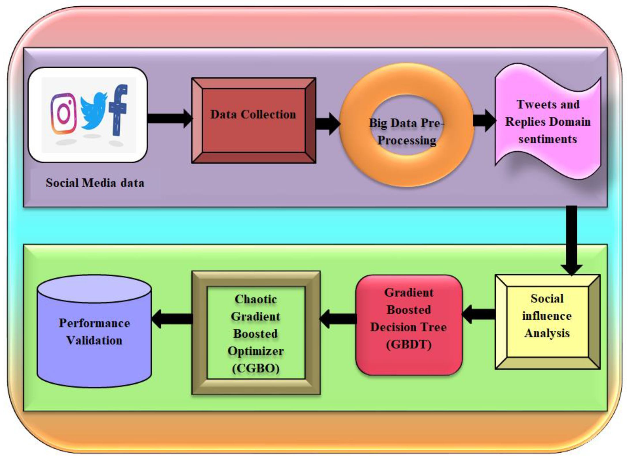
This section explains the proposed framework’s overall layout as well as the operations that form the influencer prediction process. Particularly, the process phases cover a wide range of prediction topics, such as data gathering, data modelling, data transformation, training and evaluation. Additionally, each of these stages can be further broken down into one or more tasks, each of which corresponds to a different method and tool for data analysis (such as machine learning and data mining approaches), which are discussed in more detail below. The workflow for influencer prediction is shown in
Figure 1, along with the tasks that must be carried out at each stage. The suggested structure is not dependent on any particular data processing method, hence it is meant to be all-inclusive. As a result, we may choose and employ a number of data analysis techniques and tools in our framework based on the algorithmic approach used to identify the most important members.
3.1. Influence in Society
Since influence is such a broad concept, there is some disagreement over how to define it in both business and academia. Some people view user influence as a measure of their popularity, while others see it as a reflection of their OSN involvement. However, there are significant changes that must be recognized in order to devise a new method for determining who the dominant people in a community are.
The effect of group members can be measured in the context of OSN-defined social groups using a metric that makes use of group knowledge, such as member behaviors or information from their profiles [
18]. In this article, we describe a member’s impact as her ability to draw others’ attention to herself as a result of her participation in a certain activity. User profiles are not taken into consideration in our study; instead, we simply pay attention to the behaviors of group members. The fact that the majority of profile information is private and inaccessible has an impact on this choice. The actions of a group can be categorized as either active or passive. Other group members cannot see passive actions because they solely consist in reading messages, browsing comments and answers, or clicking on a group link. They are not covered since they are outside the purview of this essay. Instead, we will focus on taking obvious action that is visible to everyone (such as publication of content, comments, replies, reactions, etc.).
Let the collection of interactions between G group members over the length of time T be denoted by ET. The influence measure IET (u) of a group member is defined by the function IET: G IR that gives u, G a numerical value. This metric shows how much a group member affects the other group members’ behaviors throughout the course of time T, resulting in a sizable number of interactions in ET. The most influential group members can be found by comparing their influence ratings after the impact measure for each group member has been determined.
Due to the intricacy of OSN, the influence measure is frequently computed by merging numerous variables. A measure of influence may consider both the structural qualities of the group as a whole and the local features of the group members (such as the types and volume of contacts they have with other members) (e.g., how important a member is to the group or how long it takes for information to spread because of a member).
Figure 1 depicts the planned GBDT-CGBO block diagram. The diagram clearly shows how social media data is collected as input and preprocessed for further optimization. Preprocessing is a practice in data mining that cleans and organizes raw data for subsequent usage. This process eliminates data anomalies or duplication that might otherwise reduce a model’s accuracy. Additionally, proper data preparation ensures that no missing or incorrect values exist as a result of human error or software flaws. For sentiment analysis, the tweet replies are taken into consideration.
Following this, the data is evaluated for social influence and categorized using the GBDT algorithm, as illustrated. Gradient-boosted decision trees are a machine learning technique for improving a model’s prediction value through repeated learning steps. The classified data is then further optimized with the CGBO optimizer and the finished data is tested to demonstrate its superior performance over the other methodologies.
3.2. Gradient Boosted Decision Tree Algorithm (GBDT)
Following this, we present our gradient boosting approach, which is based on a boosting tree. The following are the procedures:
Step 1: Initialize .
Step 2: Perform the following to calculate the residual for each
m = 1, 2, …,
M:
Step 3: Learn a regression tree by fitting . The output is .
Step 4: Update
, where
and obtain the gradient tree for the regression problem:
GBDT Algorithm
Finally, we show our GBDT method in the following manner.
Step 1: Initialize a weak learner.
Step 2: For each m = 1, 2, …, M:
Step 2(a): For each sample
i = 1, 2, …,
N, calculated the residual (i.e., negative gradient) as follows:
where
Step 2(b): Consider the residual, rim, as the new value and xi and rim as the training data for the following tree for each i = 1, 2, …, N. Assume that is the new regression tree and that represents the regions of its leaf nodes, where j = 1, 2, …, J. j stands for the number of leaves in the specified regression tree in this case.
Step 2(c): Calculate the corresponding optimal fitting value as follows for each
j = 1, 2, …,
J:
Step 2(d): Create a model for increased learning as follows:
Step 3: The completed model should look like this:
3.3. Chaotic Gradient-Based Optimizer
The purpose of this chaotic method is to improve the quality of search for the global optimum by decreasing the likelihood of becoming locked in a “local optimum”. As a result, chaos theory is being used for a variety of optimization problems. Chaos can be used to determine the optimum answer if the FS problem is described as an optimization problem with a search space of 0 to 1.
A GBO [
18] can identify optimal solutions to difficult optimization problems by combining population-based and gradient-based methodologies [
18,
19,
20,
21]. The GBO method navigates the issue space using Newton’s method and puts the search agent in the proper direction [
22,
23,
24,
25]. The gradient search rule and the locality escaping operator are crucial to the success of the GBO method [
26,
27,
28,
29].
3.3.1. Initialization Stage
As was previously stated, the GBO method [
30,
31,
32] uses a uniform distribution of initial solutions, after which the positions of the agents are adjusted in the gradient’s favor [
33,
34,
35,
36,
37]. A critical component is used to establish a balance between exhaustively investigating all feasible solutions and accepting substandard ones [
38,
39,
40,
41,
42].
where
Y is the decision variable,
and
are the bounds and
rand(0,1) as in Equation (8) is a random number between 0 and 1.
3.3.2. Gradient Search Rule Stage
In exploration and exploitation activities can be balanced by modifying the parameter in line with the sine function.
While
N is the total number of iterations and n is the current iteration number,
and
are constant values of 0.2 and 1.2, respectively. This option’s value changes between iterations [
43,
44,
45,
46,
47]. To encourage population variance, it starts with a high value in the early optimization rounds. In order to hasten population convergence, the value is subsequently decreased over a number of repetitions [
48,
49,
50]. The parameter value steadily rises within a predetermined range, expanding the variety of potential solutions and selecting the best that allows for further exploration. As a result, it is now feasible to stop local sub-regions [
51,
52,
53]. There are several techniques to calculate GSR:
Equation (13), which demonstrates how to calculate the random offset that exchanges the dissimilarity between the optimal solution (
) and a randomly picked solution (
), is shown above in Equation (12). Based on equation, the variable’s
meaning is modified in Equation (15). The following equation incorporates a second random integer during the exploration phase.
where a random vector with a range of (0,1) of
M items is designated by the symbol rand (1:
M). Two parameters,
and
, are used to measure the phase scale and decide it “step-wise”. Four numbers (
) picked at random differ from one another.
When directional tonal movement (
DM) is used, the
space of solutions converges. The
DM provides a realistic search direction that greatly affects GBO convergence by altering the current vector (
) to point in the direction of the most viable
.
where
is a uniformly distributed random parameter that determines the length of each vector agent’s stride and
rand is an integer with the same distribution. Important components of the GBO exploration process are taken into account by the
parameter. The following formula is used to compute the
parameter:
The location of the current vector (
) is then modified using variables
GSR and
DM by applying Equations (18) and (19).
where
is the vector that has been changed as a result of modifying
. The
can be recast using Equations (11) and (12) as follows:
where the vectors
and
of the current solution are
,
and
and
,
, respectively, are equal to the average of the two vectors. This is calculated using the following formula:
and
denote the worst and best solutions, whereas
and R represent both the current solution vector and a random solution vector of dimension
n. The calculation above demonstrates how to replace the current solution vector,
, with the optimal solution vector,
:
The following equations are used to enhance the GBO method’s exploration and exploitation stages. In this search method, the exploitation process is given precedence. Equation (20) serves local searches better, while Equation (21), serves worldwide searches better Equation (19). For the next iteration, the following response is preferable:
and
are two random numbers, each falling between [0, 1].
is calculated as follows:
3.3.3. Local Escaping Operator Stage
The Local Escaping operator would improve the proposed GBO algorithm’s ability to handle complex problems (), successfully updating the solution’s position by the . As a result, the convergence to a global optimum is sped up. The incorporates a variety of methodologies, including (the best position, the solutions randomly selected from population , and randomly generated solution , ). The method is applied in accordance with the following suggestions, effectively refreshing current solutions.
is a random number from a normal distribution with a mean of zero and a standard deviation of one, whereas
is a uniform random number in the range [0, 1]. The definition of probability is pr. Three random numbers,
,
and
, were produced as follows:
If
is a number in the range [0, 1], then
rand is a random number from the range number ∈ [0, 1]. The previous
,
,
equations can be simplified as follows:
where
is a parameter with two possible values (0 and 1) and is 1 if
is less than 0.5 and 0 otherwise. It is advised to follow the steps below to find the solution
:
is a randomly generated solution in the formula:
In the [0, 1] range, is a chance number and the algorithm reflag provides a straightforward explanation of the GBO method’s pseudo-code.
An N-dimensional chaotic map has the following properties:
CGBO employs a variety of maps, including Chebyshev, circular, logistic, Guass/Mouse, piecewise, sine, singer, sinusoidal and tent maps. If these maps operate as anticipated, the GBO’s productivity and convergence rate could be greatly increased. To ensure that each iteration of the proposed algorithm performs as expected, the results must be evaluated at various stages throughout the process. The CGBO’s fitness function is broken down into its essential pieces below.
where
Fitness > T;
R stands for classification error rate,
C for the total number of features in the dataset,
α for relative importance of classification quality, and
β for subset length, which is specified in the range [0, 1];
G represents the group column of the classifier; T stands for the circumstance in which each method is assessed using the fitness function. To maximize the solution, the objective function must be greater than T.
4. Results and Discussion
To conduct the online study of the social context in which the news is delivered, a survey asking real people to judge the trustworthiness of specific Twitter identities was created. Profiles of real persons or websites were displayed to users, with selection based on how much bogus or real news they shared throughout the dataset’s collection phase. At random, each user was assigned five extremely trustworthy profiles and five extremely untrustworthy profiles.
The experiment is carried out on a computer running the Windows 7 operating system and an I5 dual core while using the PyCharm integrated development environment. The Lastfm dataset and the CiaoDVD dataset are used to assess the trained models. 17,615 users, 16,121 films, 72,665 interactive user and film records and 40,133 user social records make up the movie dataset known as CiaoDVD. The ratings range from 1 to 5 and users tend to favor films with higher ratings. The users’ social connections serve as a proxy for their friendships. Even though there are many ratings, the movie dataset is still sparse—at about 0.0256%. In total, 1892 users, 17,632 songs, 12,717 social records for users, 92,834 music records of users and 11,946 tags make up the Lastfm music dataset. The music dataset is sparse to a degree of about 0.2783%.
The confusion matrix assists practitioners in judging whether the outputs are of good quality. Patients who had heart disease and were correctly diagnosed were labelled as true positives (TPs), while those who did not have the disease were labelled as true negatives (TNs), while those who did not have heart disease were labelled as false negatives (FNs) and those who did not have heart disease were labelled as false positives (FPs). In medicine, the most harmful forecasts are those that result in false negatives. The different performance metrics were created with the use of a confusion matrix. Accuracy was determined using instances that were correctly identified (Acc). The accuracy is calculated from the Equation (35)
Precision was defined as the positive prediction value by
The proportion of individuals with cardiac disease identified by recall
The F1 score took into account a harmonic average of precision in Equation (36) and recall in Equation (37) defined by
The Root Mean Squared Error statistic can be used to determine how far actual results differ from estimates (RMSE). Its value can be calculated using Equation (39).
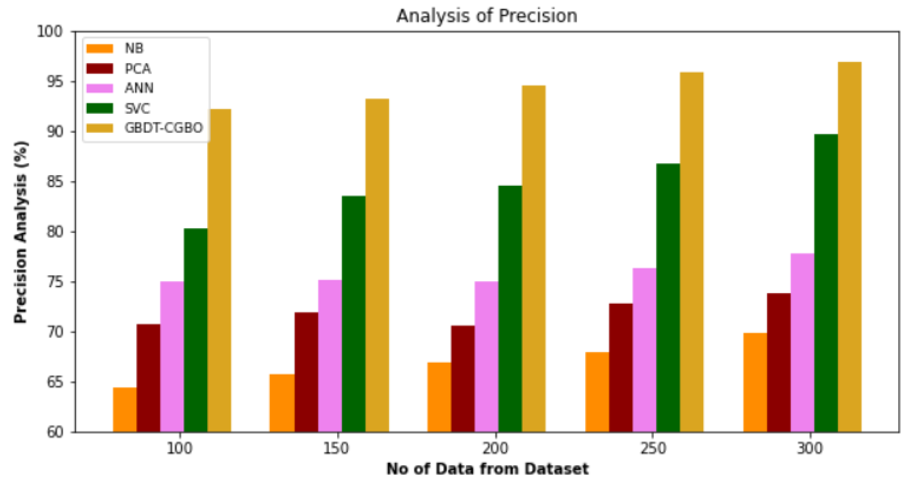
4.1. Precision Analysis
A comparison of the precision of the GBDT-CGBO approach with other existing approaches is shown in
Figure 2 and
Table 1. The graph demonstrates that the network technique has led to improved performance and accuracy. For instance, the GBDT-CGBO model has gained 92.25% for data, compared to NB, PCA, ANN and SVC with 64.32%, 70.72%, 74.94% and 80.23%. However, the GBDT-CGBO model has shown maximum performance with different data sizes. Similarly, under 300 data, GBDT-CGBO achieved 96.92% whereas NB, PCA, ANN and SVC models gained 69.83%, 73.84%, 77.84% and 89.65%, respectively.
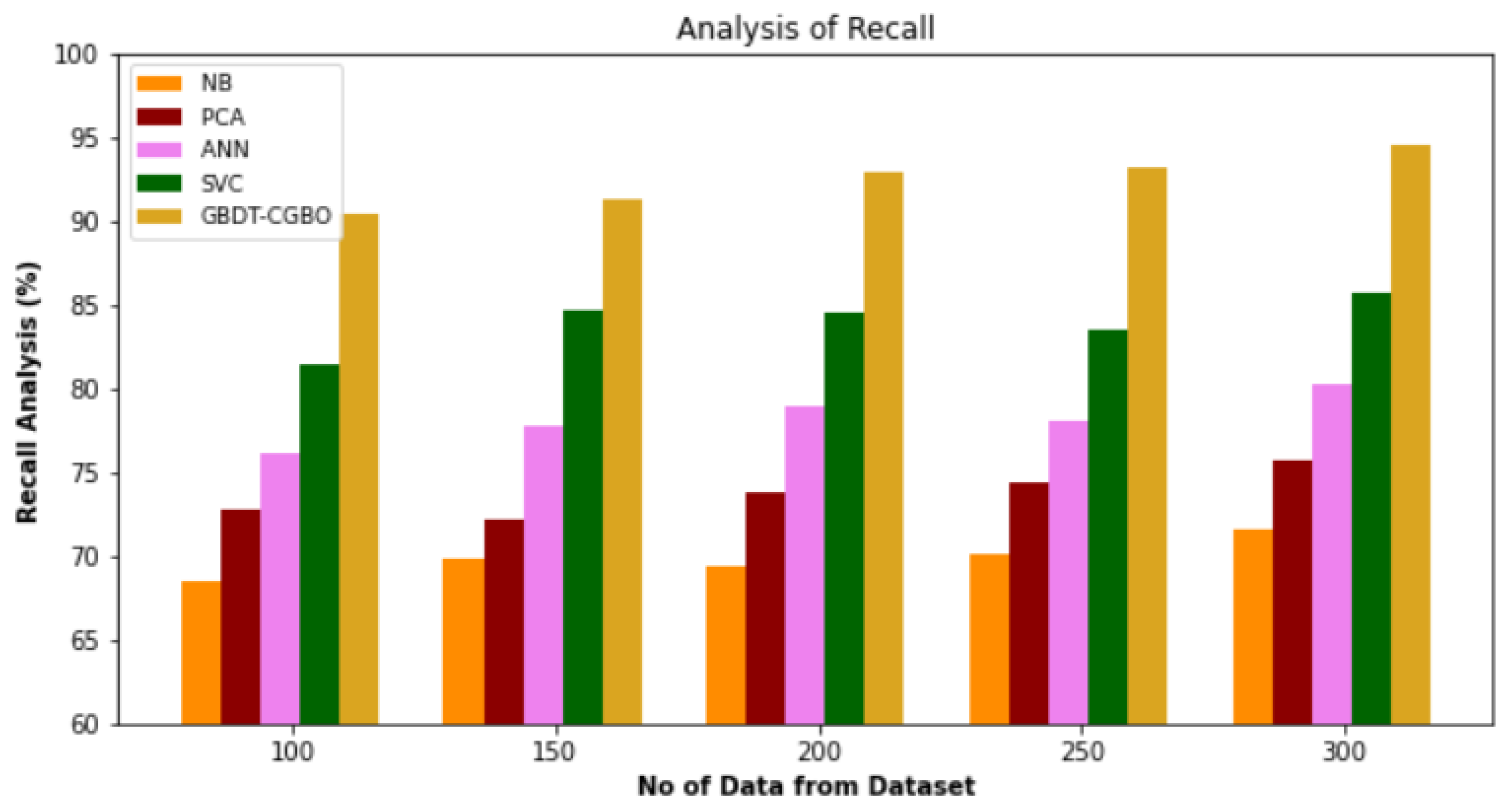
4.2. Recall Analysis
Figure 3 and
Table 2 demonstrate a recall comparison between the GBDT-CGBO strategy and other approaches in use. The graph demonstrates that the network technique led to improved performance with recall. For example, with data 100, the GBDT-CGBO model gained 90.45% recall, whereas the NB, PCA, ANN and SVC models obtained recall of 68.54%, 72.84%, 76.13% and 81.41%, respectively. However, the GBDT-CGBO model has shown maximum performance with different data set sizes. Similarly, under 300 data GBDT-CGBO achieved 94.54%, whereas NB, PCA, ANN and SVC models achieved 71.67%, 75.64%, 80.32% and 85.76%, respectively.
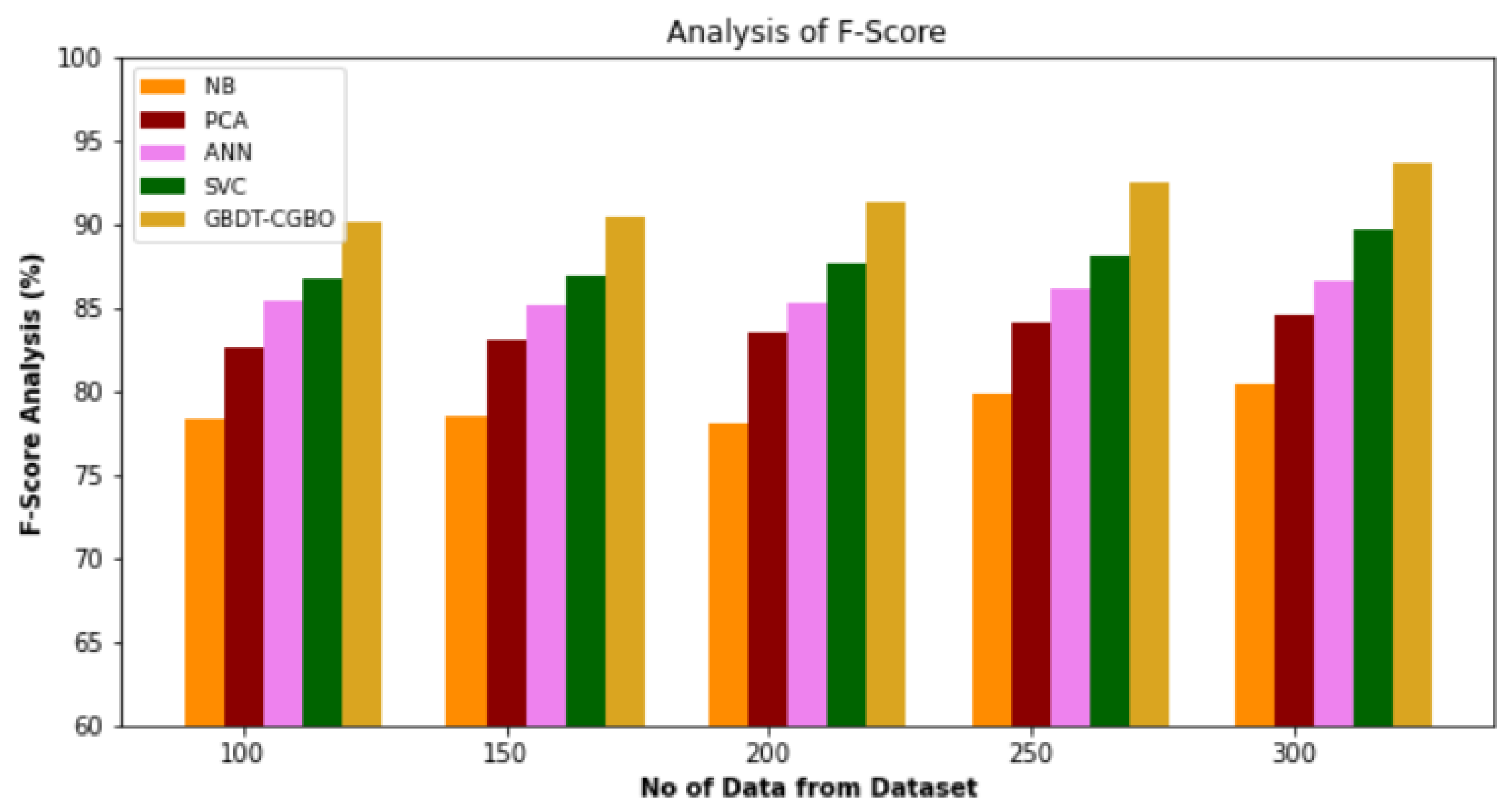
4.3. F-Score Analysis
Figure 4 and
Table 3 present a comparison of the GBDT-CGBO strategy and other existing methodologies using F-score analysis. The graph demonstrates that the network strategy led to improved performance as measured by the F-score. For example, with data 100, the F-score value is 90.12% for GBDT-CGBO, whereas the NB, PCA, ANN and SVC models have obtained F-scores of 78.43%, 82.65%, 85.45% and 86.74%, respectively. However, the GBDT-CGBO model has shown maximum performance with different data size. Similarly, under 300 data, the F-score value of GBDT-CGBO is 93.67%, whereas NB, PCA, ANN and SVC models achieved 80.43%, 84.54%, 86.56% and 89.74%, respectively.
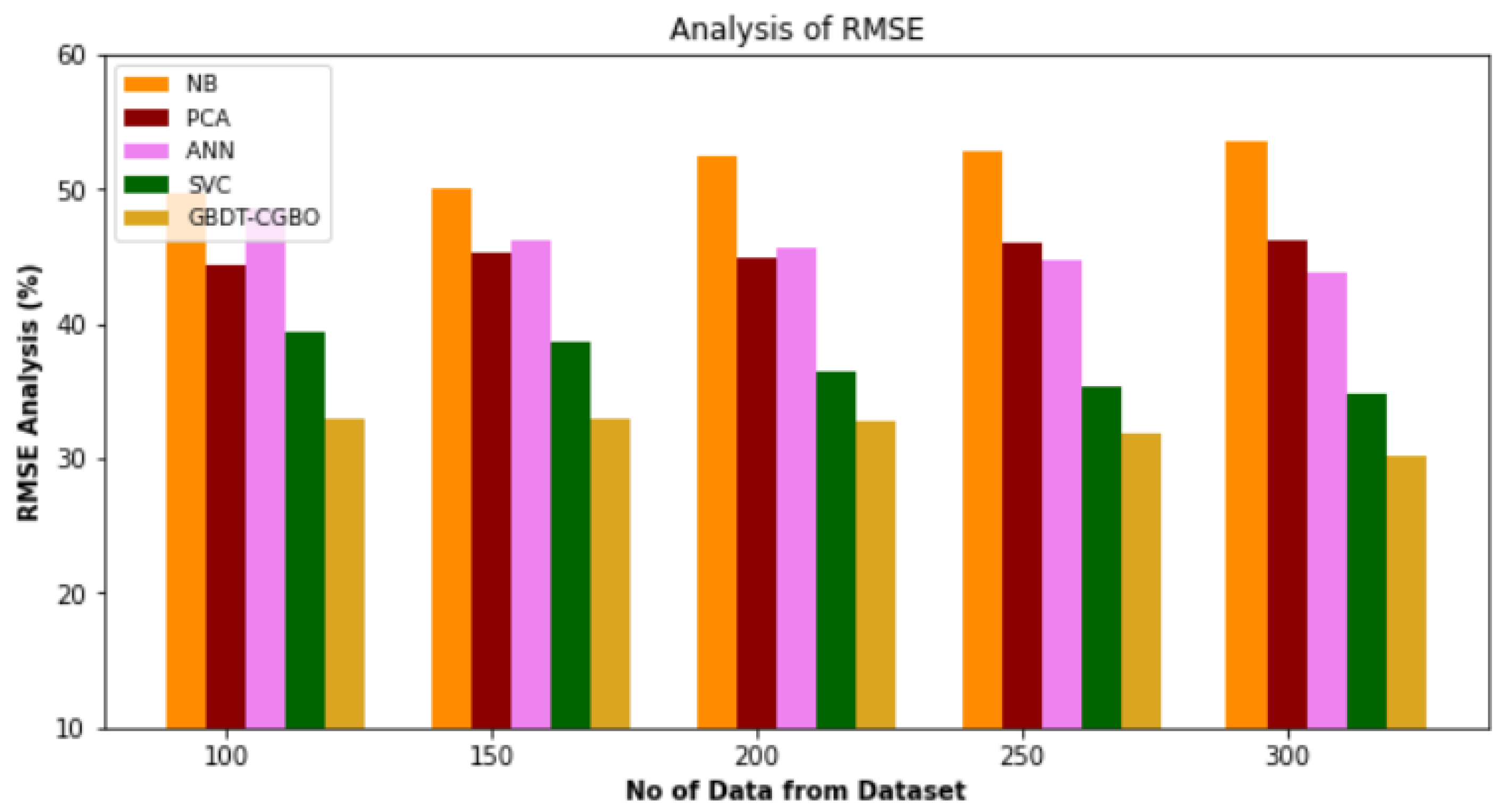
4.4. RMSE Analysis
Figure 5 and
Table 4 demonstrate an RMSE comparison of the GBDT-CGBO approach against various available techniques. The graph demonstrates that the network strategy led to improved performance with a lower RMSE value. For example, with data 100, the RMSE value is 32.91% for GBDT-CGBO, whereas the NB, PCA, ANN and SVC models have slightly enhanced RMSE of 49.74%, 44.35%, 48.54% and 39.43%, respectively. However, the GBDT-CGBO model has shown maximum performance for different data sizes with low RMSE values. Similarly, under 300 data, the RMSE value of GBDT-CGBO is 30.21%, while it is 53.65%, 46.28%, 43.72% and 34.76% for NB, PCA, ANN and SVC models, respectively.
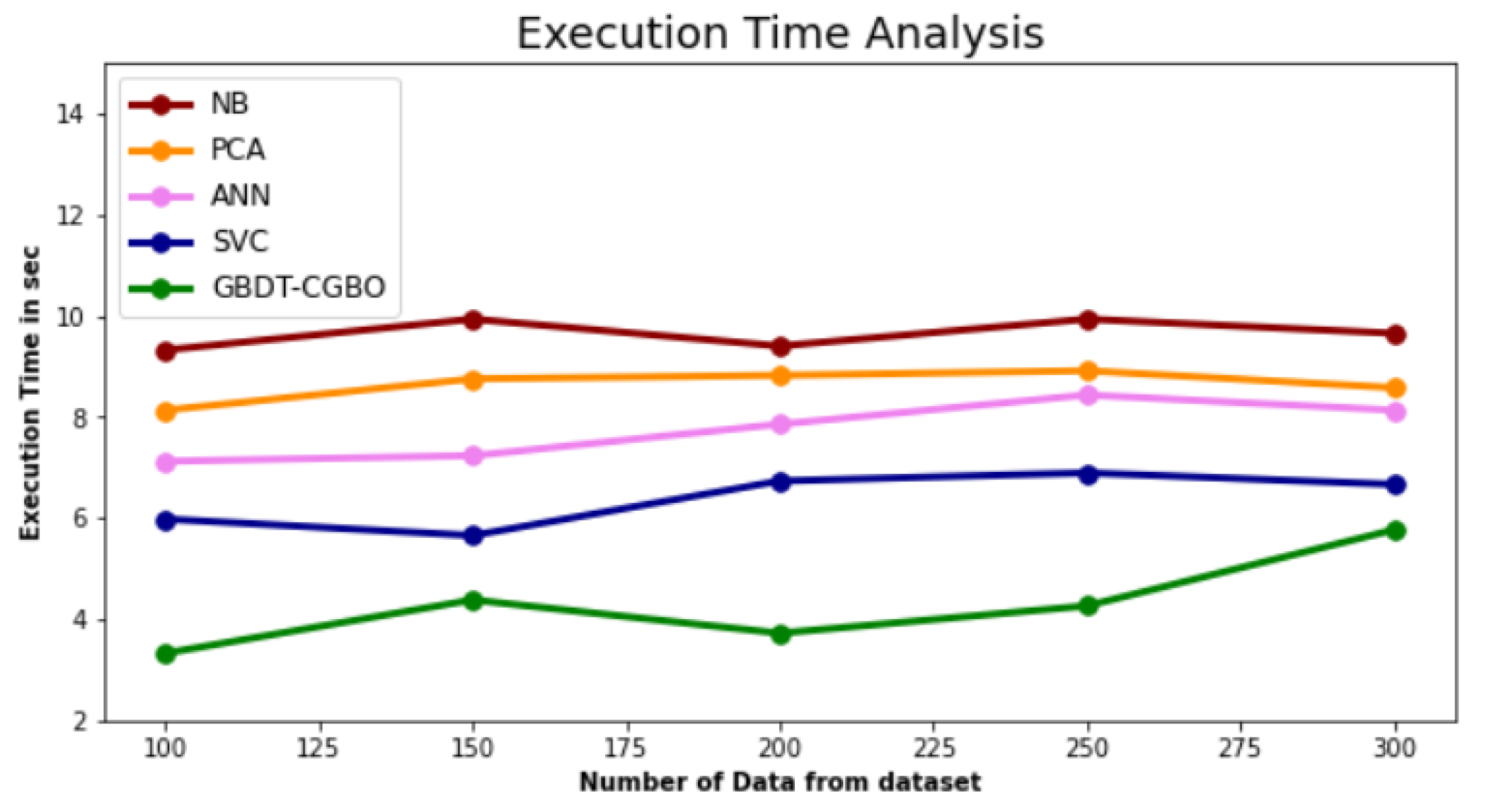
4.5. Execution Time
In
Table 5, how the GBDT-CGBO technique’s execution time compares to that of existing techniques is detailed. The data clearly shows that the GBDT-CGBO method has outperformed the other techniques in all aspects. For example, with 100 data, the GBDT-CGBO method has taken only 3.327 s to execute, while the other existing techniques such as NB, PCA, ANN and SVC have an execution time of 9.321 s, 8.632 s, 7.123 s and 5.980 s, respectively. Similarly, for 300 data points, the GBDT-CGBO method has an execution time of 5.765 s while the other existing techniques such as NB, PCA, ANN and SVC have taken 9.652 s, 8.576 s, 8.132 s and 6.665 s of execution time, respectively as shown in
Figure 6.
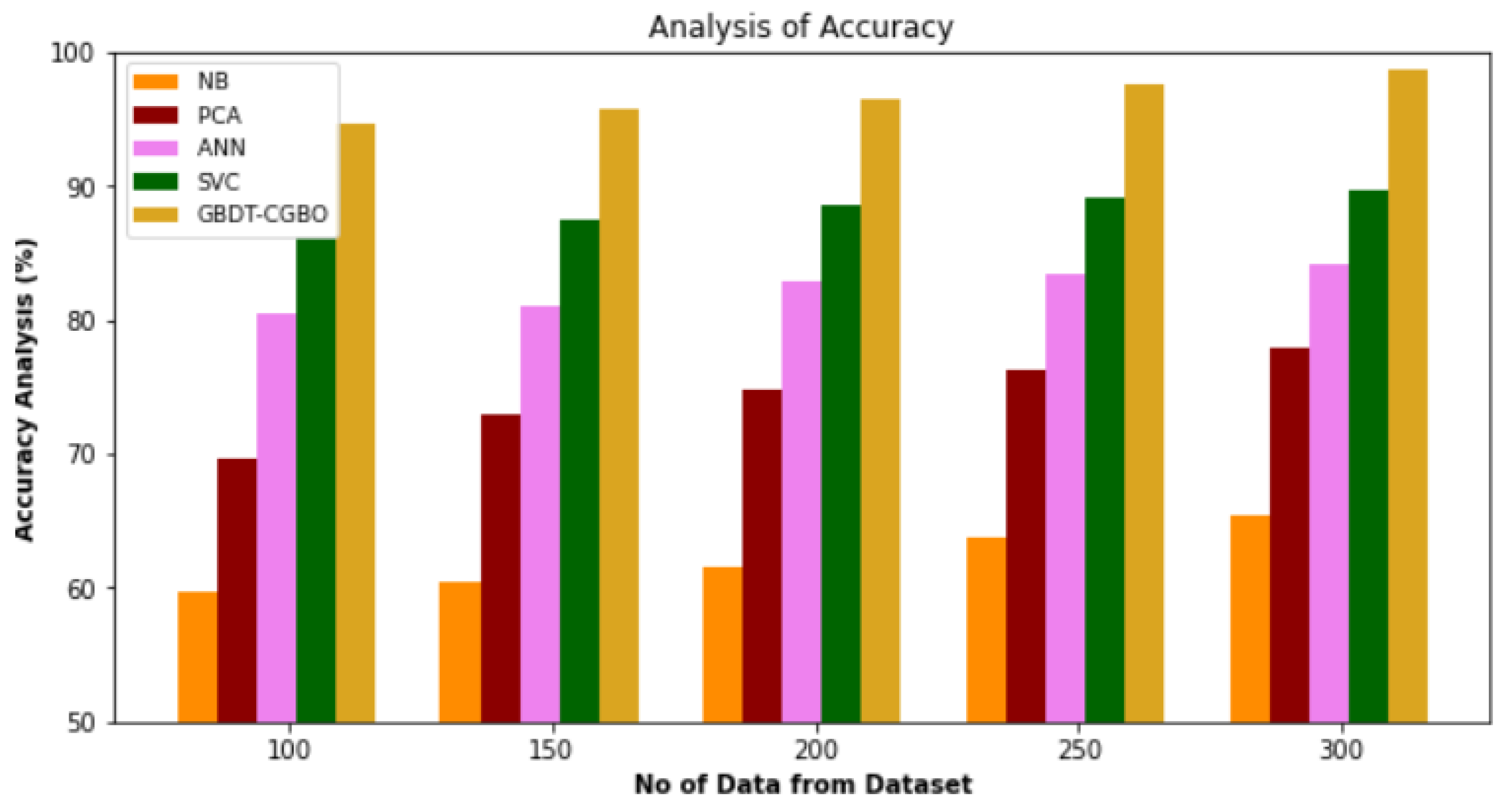
4.6. Accuracy Analysis
Figure 7 and
Table 6 provide a comparison of the GBDT-CGBO approach’s accuracy with other existing approaches. The graph illustrates that the network technique resulted in improved performance and accuracy. For example, with data 100, the accuracy value is 94.65% for GBDT-CGBO, whereas the NB, PCA, ANN and SVC models have obtained an accuracy of 59.76%, 69.65%, 80.54% and 86.15%, respectively. However, the GBDT-CGBO model has shown maximum performance with different data set sizes. Similarly, under 300 data, the accuracy value of GBDT-CGBO is 98.76%, while it is 65.45%, 77.89%, 86.56% and 89.72% for NB, PCA, ANN and SVC models, respectively.
5. Conclusions
The study mentioned set out to look into the factors that can be used both automatically and manually to identify social network profiles that spread false information. We worked on two levels to accomplish this goal: first, we extracted and used criteria related to news content to classify it as authentic or false. After that, we worked on identifying elements like social, personal and interaction data with both content and other users to ascertain the news-sharing reliability of the observed users. The GBDT-CGBO framework was introduced in this review, along with a helpful mechanism for identifying users who may be able to influence the behaviour of others in the future based on prior interactions within the group. Our contribution is backed up by a sizable experimental effort, strong logic and tried-and-true analytical methods. It is supported by a large experimental campaign, sound reasoning and accepted analytical techniques. Data was collected on the interactions of approximately 800,000 people from 18 different Facebook groups to assess the accuracy of the projections. The results demonstrate how effective and practical our GBDT-CGBO strategy is. Under 300 data points, GBDT-precision CGBO’s value is 96.92%. With 100 pieces of data, the GBDT-CGBO method only took 3.327 s and with 100 pieces of data the recall value for GBDT-CGBO is 90.45%, the F-score value is 90.12%, the RMSE value is 32.91% and the accuracy value is 94.65% for GBDT-CGBO. The experimental evaluation results show that, with an average accuracy of 98.76%, the objective of differentiating false news from legitimate news has been achieved for content categorization. AUC is the most popular measure of novel proposed approaches. Future studies should measure novel methodologies unless other conditions can be met. Rapid growth, sparseness and network properties are link prediction problems. Much real-network data, like online social networks, is dynamic and sparse. Link prediction must avoid isolated node cold-start difficulties. Using tags and time to increase forecast accuracy is another difficulty. To address these issues, future research must shift its focus away from online social networks and toward link prediction in co-authorship networks and economic networks. The rise in scientific publications encourages co-authorship networks and strengthens author relationships.


 ,
, 


