Improving Real Estate Rental Estimations with Visual Data

Abstract

Multi-modal data are widely available for online real estate listings. Announcements can contain various forms of data, including visual data and unstructured textual descriptions. Nonetheless, many traditional real estate pricing models rely solely on well-structured tabular features. This work investigates whether it is possible to improve the performance of the pricing model using additional unstructured data, namely images of the property and satellite images. We compare four models based on the type of input data they use: (1) tabular data only, (2) tabular data and property images, (3) tabular data and satellite images, and (4) tabular data and a combination of property and satellite images. In a supervised context, the branches of dedicated neural networks for each data type are fused (concatenated) to predict log rental prices. The novel dataset devised for the study (SRED) consists of 11,105 flat rentals advertised over the internet in Switzerland. The results reveal that using all three sources of data generally outperforms machine learning models built on only tabular information. The findings pave the way for further research on integrating other non-structured inputs, for instance, the textual descriptions of properties.

1. Introduction

Designing models that simultaneously consider various data forms has become increasingly important in recent years. Incorporating assorted forms of unstructured data, such as images and textual descriptions, has been the focus of many studies [1,2,3]. However, coalescing structured and unstructured data remain largely unexplored. The process of interfusing various data forms has been referred to in different ways depending on the field and scope: multi-modal learning [4], multi-view learning [5,6], and multi-input learning [7,8]. The appropriate terminology for amalgamating structured and unstructured data in pursuit of a supervised goal is open to debate. In this paper, we refer to this phenomenon as multi-modal learning. Our work sheds light on the application of multi-modal learning for the real estate industry and automated valuations models (AVMs) that can democratize the valuation process for the consumers.

The real estate industry is one domain that can significantly benefit from coalescing different data types. Property price estimation—often said to be more of an art than science—involves an abundance of data in various forms, thereby making it ideal for multi-modal learning. Professional appraisers consider many conventional and tangible factors when evaluating properties. Nevertheless, many automated pipelines and modeling approaches ignore intangible factors that significantly influence a buyer’s or renter’s decision. In addition to misleading the consumers, professional appraisers may fall victim to the wrong valuations as AVMs become indispensable for nourishing the growth and scalability of the appraiser’s operations. Moreover, in an inefficient setting such as real estate, it is imperative to harvest the value of internal and external data whereby the existing features are engineered into a holistic approach capable of producing accurate valuations. Similar to a human’s cognitive ability, the design of AVMs should allow the models to assess different content before generating valuations.

The attributes influencing the price of the property have been the topic of several research studies [9,10,11,12]. Most studies model this phenomenon through conventional hedonic pricing models, where regression analysis is applied to assess the importance of various features in predicting real estate prices. This includes easily measured attributes such as the number of rooms, the size of the house, and the year of construction [9]. The selection of such attributes is often a complex process and highly depends on the local market under the study [10]. In general, such attributes are characterized according to the information they provide: (i) the structure, (ii) the general location, or (iii) the neighborhood and the immediate surrounding environment [11,12].

One prominent form of unstructured data readily available to real estate seekers is properties’ interior and exterior images. While visual cues may impact the prices, accurately describing them in structured formats can be challenging. There have been a few studies that model property sales prices through such property images. Poursaeed et al. [13] focused on estimating luxury levels through a semi-supervised model combining both annotated structured visual cues from a crowd-sourcing platform with the tabular data as inputs to a support-vector machine (SVM). In a similar work, Ahmed and Moustafa [14] used frontal images of houses, bedrooms, kitchens, and bathrooms to extract visual features through the speeded up robust features (SURF) algorithms. Their findings showed that images could significantly improve price estimations where neural networks (NNs) outperform SVMs. Furthermore, Lee and Park [15] revealed that more recent deep learning techniques might outperform SURF by using only the tabular features and exterior images of a property without a separate algorithm for feature extraction. Zhao et al. [16] simultaneously considered luxury levels such as AVA scores [17] and property images to build hybrid machine learning models for price predictions.

The property images found in online announcements can capture structural information; however, the 2D satellite images of the property are arguably better for understanding the neighborhood’s aesthetics and the immediate surroundings of a given property. Law et al. [11] looked at the effect of adding panoramic street view (referred to as aerial) and satellite images to tabular features for improving price estimations, where two approaches are noteworthy to highlight the integration of visual information. In both approaches, convolutional neural networks (CNNs) extracted visual cues from the two image types as two different functions. The difference between the two approaches is that in one, the outputs of these functions were concatenated with the standard tabular attributes processed by a separate NN. In contrast, the second technique used visual desirability scores produced by the CNNs as inputs to a more interpretable model (linear or additive) to understand individual contributions better. Their results showed that both models outperformed the simple linear approaches and the NN, in particular, generated the best estimations. Furthermore, Kucklick et al. [18] used the satellite images and tabular features to demonstrate the power of concatenating multiple inputs and discussed how multi-view learning could help outperform models with isolated inputs. Finally, Bency et al. [19] showed that transfer learning and NNs can outperform spatial auto-regressions (SAR) and other models due to their ability to fuse visual cues from satellite images with typical property attributes.

Our work assesses the value of unstructured data for real estate modeling. We examine a combined usage of images related to the property (interior and exterior and satellite images) and structured information. To our best knowledge, our research is the first attempt to combine these two sources of visual information in a single real estate model. Furthermore, the aim is to understand whether such multi-input models can outperform conventional modeling approaches that operate only on structured data.

Research Question

This paper evaluates the effect of multi-modal learning in the form of images and tabular information. Therefore, the research question consists of two parts:

• Does the performance of a neural network that uses tabular features for predicting rental prices improve with additional training data that are non-structured, including advertised property images and satellite views?
• Does such a neural network outperform models trained solely on structured features?

The remainder of this paper is as follows: Section 2 describes our real estate datasets and the pre-processing applied to both the structured information and the images. In Section 3, we outline the methodology applied for multi-modal learning to predict the log rental prices. In Section 4, we outline our empirical results by highlighting the performance of each model. Additionally, the same section derives our findings and their implications. Lastly, in Section 5, we summarize and conclude the main findings while shedding light on the limitations of our work.

2. Swiss Real Estate Dataset

Finding publicly available datasets where images and tabular attributes for real estate listings co-exist is challenging. For this paper, the dataset of listings was gathered from a Swiss real estate platform. The platform contains property advertisements in Switzerland and its neighboring cross-border cities. The announcements are published by private individuals and real estate agencies, expanding over several listing categories. Most notably, an announcement may involve selling or renting different property types such as flats or houses. Among these, flat rentals had the highest number of announcements. While the platform and its structured property features were translated and made available in four languages (English, French, German, and Italian), the unstructured description of the property often remained in the original language of the publication.

Our dataset, named SRED (Swiss Real Estate Dataset), consists of 17,758 flat rentals scraped in English during February and March 2021. Each listing contains a price, which may refer to rental price or sales price depending on the type of listing. Additionally, throughout this paper, the term price has been used for rental prices.

2.1. Tabular Data

SRED contains 12 structured and unstructured features, some of which may be relevant for flats. The structured features that are suitable for both property types (flat or house) are the price, living space (${\mathrm{m}}^2$), number of bathrooms, number of rooms, location (longitude and latitude), year of construction, and advertiser (private contact or agency details). Additionally, there are common unstructured features in the form of a title for the announcement, attached property images, and a description of the advertisement. Some features are only meaningful and relevant based on the property type. For instance, a flat may have a feature indicating the floor number on which it is located.

While the primary aim of this paper is to use all predictive features, the heterogeneity in the available data played an essential role in the final selection of adequate modeling features. Some scraped features were frequently missing due to inconsistency in HTML tags and were often misplaced by the user. The chosen consistent and informative features include the living space, number of bedrooms, and location. The literature also supports this choice of variables [9].

The inclusion criteria of a listing are of two types. Firstly, and the methodology dictates that listings must (i) report the exact address to obtain location features, (ii) have a year of construction < 2020, since those ≥ 2020 were assumed under construction, and (iii) have at least four property images, since this is central to the modeling process. Secondly, listings must (vi) have a surface of at least 18 ${\mathrm{m}}^2$, (v) have rental prices between CHF 200 and 7500, and (vi) have to be located in Switzerland and its cross-border cities ($5\le$ longitude $\le 12$ and latitude $\le 45$).

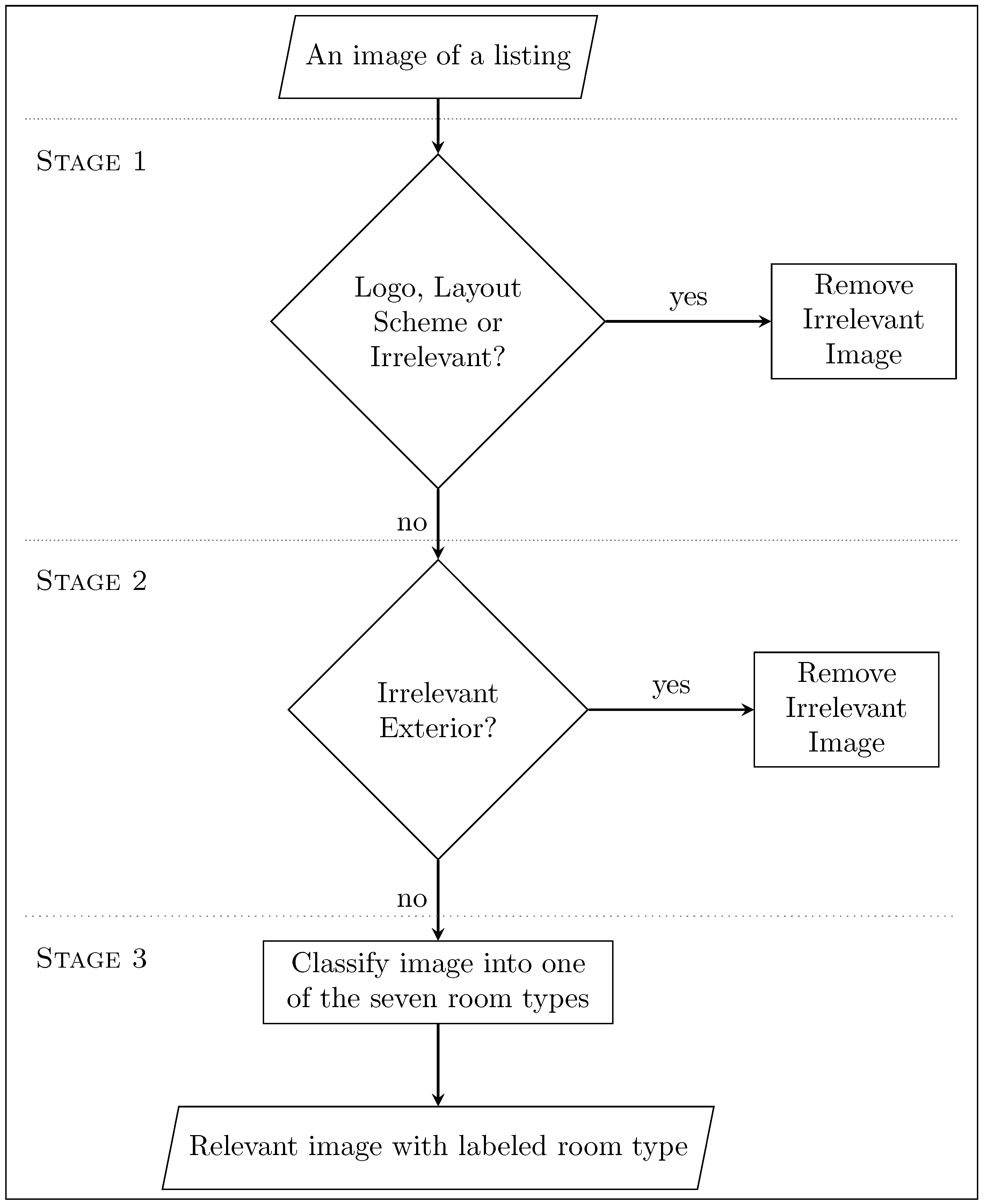
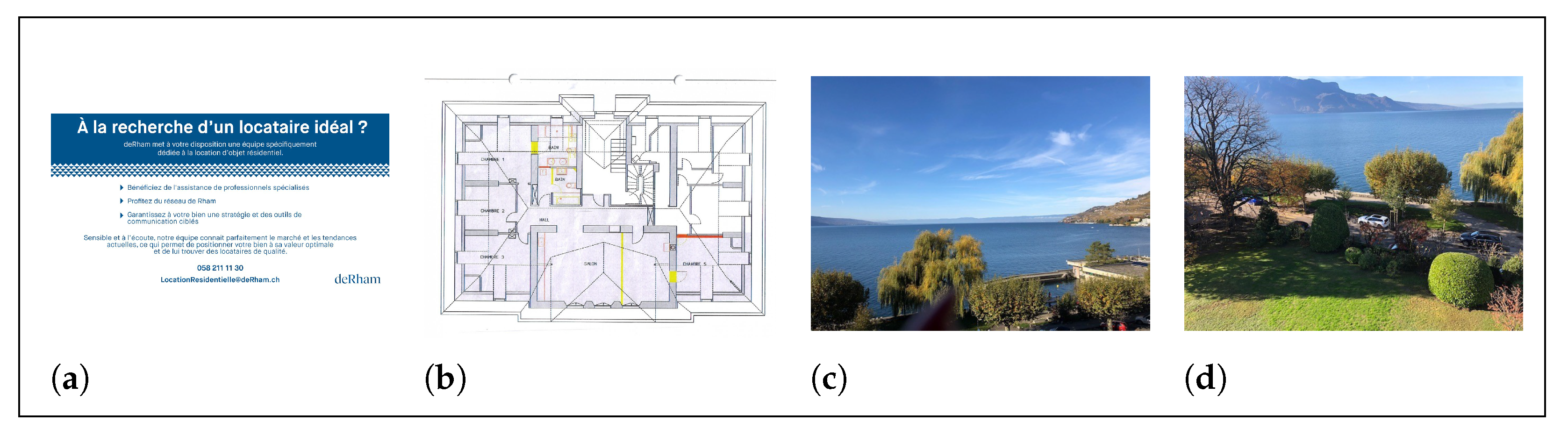
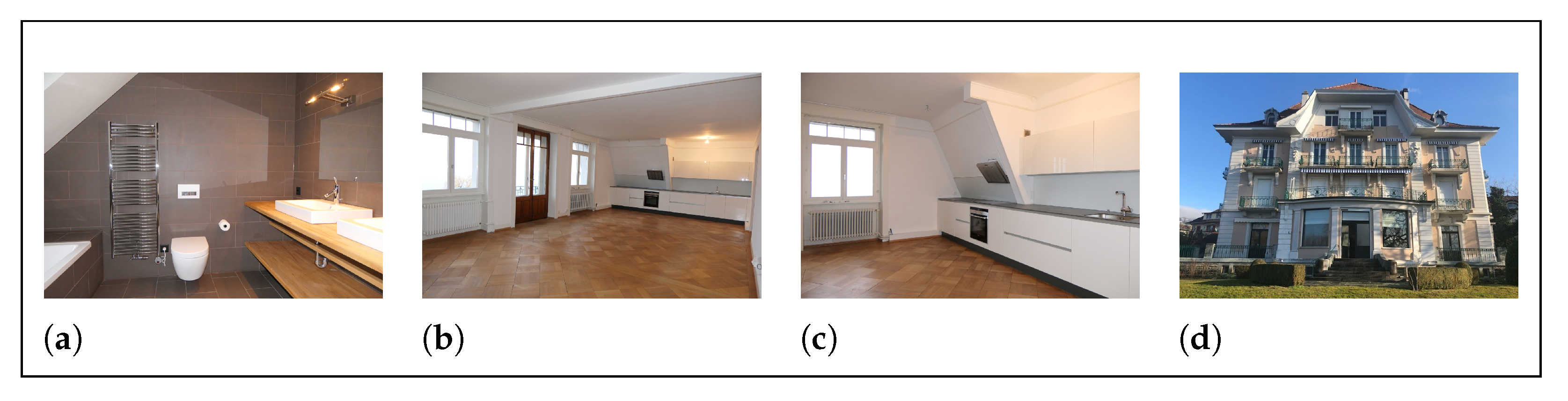
2.2. Image Data

Each listing in SRED contains a set of images attached by the advertiser. The real estate platform assumes that these images provide visual information about the property, for instance, showcasing the listing’s interior and exterior. However, some images do not directly represent a property, such as images of realtor’s logos, pets, nearby forests, and waterfalls. These images should be removed from the dataset to obtain cross-comparable images across all listings. For this purpose, we designed a three-stage process that included three classification models where we assumed that most output images were photographs. Before beginning the image pre-processing, each SRED listing had a mean of 8.42 images and a median of 8.

In the first step, images representing logos, mock-ups, the layout schemes of a rental unit or its affiliated buildings, and all images not showing the property’s appearance were removed. Indeed, a logo could bring information such as the name and contact details of the commercial realtor, which may also be provided in the tabular feature, and thus carry redundant information. Removing those prevents a pricing model from learning shortcuts on incomparable listings. Further, we included other irrelevant images (e.g., pets and persons) within the irrelevant category. In the first stage of our process, we used a binary classification model to filter such images out from our dataset.

The second type of images considered irrelevant included mostly outdoor images where the building of the flat was not identifiable. Such images primarily relate to the property’s exterior, for instance, photos taken of or from gardens, balconies, and, more generally, outdoor shots that did not include the property building. The second pre-processing stage was designed to remove such outdoor images through another binary classifier.

In the last step, the remaining relevant images were classified into one of seven categories: bathroom, bedroom, kitchen, living room, dining room, interior (miscellaneous), and exterior. To this aim, we used the publicly available datasets from Poursaeed et al. [13]. There are four key remarks with regard to these images. First, the interior class mainly represents the miscellaneous and, in our case, potentially unwanted images, such as stairs, corridors, elevators, and unusual images, that are not strictly related to the property. Second, the kitchen category contains open kitchens (no walls or barriers separate the kitchen from the living or dining rooms), like many SRED listings. Third, distinguishing between living and dining rooms may not be relevant, particularly for studios or small properties. At last, the exterior class has the most images which bear various architectural styles. This variety helps the classification model to identify the different styles of buildings. Since the dataset provided by [13] is not specific to one region while SRED is specific to Switzerland, it may be argued that some classes, such as exterior images, could benefit from images that are primarily Swiss architectural designs. In practice, such architectural styles did not seem to influence the correct identification of exterior images, as the other classes differed vastly.

We summarize our three-stage image pre-processing in Figure 1. This process was applied to each image in our dataset.

In order to train our first two binary models, two individual annotators labeled images from SRED from randomly selected listings. For the first classification task, 15,110 images were labeled, where 96% belonged to the class with relevant images. For the second classification model, there were 14,549 images, including 92% relevant images. Examples of annotated irrelevant images for these two stages have been shown in Figure 2. Additionally, it should be noted that the irrelevant images of the first model were not carried on to the second set of annotations. The images in both cases were randomly split in 95:5 proportions for training and testing. In terms of the performance on the test set, the first classification model reached a balanced accuracy of 97.5%, while the second model achieved a balanced accuracy of 94.5% for removing irrelevant exterior images. Attaining a high specificity in both cases—99.8% and 99.2%, respectively—meant that, on average, very few relevant images were removed.

We trained the classification model from the third stage based on the combination of the dataset by Poursaeed et al. [13] and images from SRED. The original dataset Poursaeed et al. (2018) used had 145,994 images of 224 × 224 pixels. We removed duplicated images from their dataset and added 2352 labeled images from SRED, yielding a dataset of 148,342 images. The annotations for SRED were performed only for the three categories of the bathroom, exterior, and kitchen, where the newly annotated images from SRED were to capture the Swiss architectural idiosyncrasies.

The images from the exterior category of [13] were incompatible with those found in SRED. This occurred because the exterior category in [13] consisted mostly of images taken from the frontal angle of the building. This meant that images from SRED, which showed a balcony or the building from a side angle, could be mistaken for another category that interests us (e.g., bathroom) since it was not included in the training set. Moreover, the images from the balcony of a property were vastly different than those from the frontal view of the building, and they deserved a dedicated category. However, as there were too few images of balconies, such images were eventually included within the exterior category. This inclusion did not pose significant challenges for answering our research question since we assumed that some irrelevant balcony images were filtered out during the second stage of image processing, that is, when deploying our second classification model for removing the irrelevant exterior images. For this task, 95% of the data was randomly taken for the training set, while the remaining 5% was used for the test set. This multi-class model reached 89.5% accuracy on the test set. The class distributions and performances are shown in

Table 1. The performance of stage on the test set separated by the room type.

Class	No Test	Balanced	F1	Sensitivity	Specificity
	Samples	Accuracy
Living room	1210	0.905	0.828	0.850	0.960
Kitchen	1217	0.937	0.899	0.892	0.982
Interior	950	0.946	0.907	0.905	0.987
Exterior	1315	0.970	0.956	0.947	0.993
Dining room	975	0.920	0.860	0.862	0.979
Bedroom	1206	0.942	0.910	0.898	0.986
Bathroom	542	0.955	0.907	0.919	0.992

. It can be observed that when considering the balanced accuracy, the best performing classes are exterior and bathroom, while the relatively worse performances are attained for living room and dining room.

To cross-compare the images from the listings, it was necessary to have a homogeneous set of room types among them. As certain room types were not found between all the listings, choosing which room types depended on what kind of rooms a human appraiser—either a professional individual or a renter—would consider predominant when comparing properties. Additionally, the choice of the room types was constrained by the available images from SRED, where certain classes may be more frequently found among the listings than others. In work by Ahmed and Moustafa [14], the authors used frontal images of houses (in our case labeled ‘exterior’), bedrooms, kitchens, and bathrooms for estimating property prices. After running the model and classifying the room types in SRED, we found the most relevant and frequent classes to be the property’s exterior, living room, kitchen, and bathroom. An example of each room type is depicted in Figure 3. It may also be argued that the appearance of certain room types such as the kitchen and bathroom may differ, while other room types such as the bedroom and living room may be similar. Therefore, in selecting relevant room types, we sought to find a balance between the frequency and diversity of the room types. Furthermore, the methodology section explains why we selected four room types.

To avoid having several images belonging to one type, we kept the image with the highest probability of belonging to that class, removing the atypical room types. There were some listings where the probability of two images belonging to the same class was very similar or the same (indicating possible duplicates), and for such cases, we selected the image with the lowest probability for its most likely alternative.

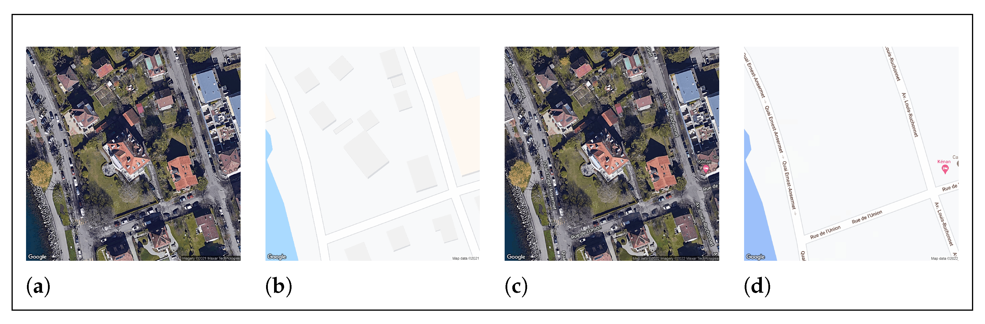
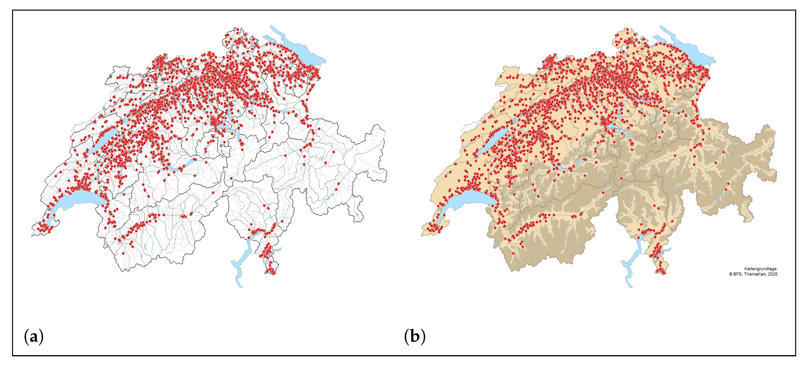
2.3. Satellite Data

Google Static Maps API was used to acquire the satellite images of real estate listings via their coordinates. The API provides four maps: roadmap, satellite, hybrid, and terrain. Although the roadmap type is probably the most recognizable, the satellite map was more relevant for this paper. As the name suggests, it represents the satellite photographs of the terrains of a given location.

We had to choose an appropriate zoom level to obtain suitable satellite images. The zoom level ranges from 0—where the entire world could be seen—to 21+—viewing the streets and individual buildings closely. We defined an appropriate zoom level as one with enough information about the neighborhood as a whole, meanwhile bearing rich information on the immediate surroundings of the target building. It is important to note that the general prices at the city level may already be reflected in the location features (longitude and latitude) and our ensuing aim was to have a zoom level leaning towards the immediate surroundings of a given listing. Through various observations, we found the zoom level of 19 to strike a good balance between the neighborhood attributes and nearby roads while maintaining a visible view of the landmark and the building.

For gathering the final SRED satellite images, for every listing, we collected a roadmap image type—without any labels of the surrounding landmarks/roads—followed by a satellite image type. Eventually, after a few early attempts, we found the satellite image type to be more effective and meaningful than artificially generated images and hence proceeded with using this map type for modeling. Examples of the four available maps are shown in Figure 4.

2.4. Descriptive Statistics of the Final Dataset

A summary of 11,105 SRED listings that remain after data processing is shown in

Table 2. Summary statistics for 11,105 SRED flat rentals after pre-processing the features.

Variable	Mean	SD	Min	Q1	Median	Q3	Max
price (CHF)	1730	598	495	1385	1620	1935	7400
living_space (${\mathrm{m}}^2$)	86	31	19	68	83	100	1502
rooms	3.589	0.941	1.5	3	3.5	4.5	14
lon	8.018	0.812	6.043	7.456	7.899	8.633	9.869
lat	47.156	0.396	45.832	46.960	47.265	47.443	47.794

. The rental prices started from CHF 495 to CHF 7400, with mean and median rentals under CHF 1800. Moreover, the smallest kind of flat was a studio flat or a property with 1.5 rooms (pièce in French). This is not the smallest possible size for a property in Switzerland, as this value could be as low as 1; however, no such property was present after pre-processing the data. Moreover, since the raw value of the price was slightly skewed, the logarithm transformation should be applied first. The resulting prices after the transformation were closer to a normal distribution and were, in turn, more suitable for the regression tasks.

All flat rental listings in Switzerland after the data selection process are shown in Figure 5, where the first map outlines all the Swiss cantons, while the second map sheds light on fertile and infertile areas. The maps indicate that the listings are geographically well spread and adequately represent the Swiss market.

3. Predictive Modeling

We considered two families of models that fall within the scope of our research question. The first group consisted of models designed for handling tabular data, such as linear regression, random forest, and neural networks. Further, we considered the models that use image data as input. Predicting prices from images alone was unlikely to produce optimal price estimations. By combining the two types of inputs—tabular information and images—we expected to see improvements in overall price predictions.

3.1. Performance Metrics

There are three relevant metrics for the regression tasks. The first two metrics, namely mean squared error (MSE) and R², are related, since minimizing MSE is equivalent to maximizing R². MSE allows us to obtain RMSE ($\sqrt{\mathrm{MSE}}$), which helps interpret the models’ monetary improvement with the large rental prices considered. R² was chosen, as it is often easy to interpret and independent of the scale of the data, beneficial to understanding the performance of our log-transformed rental prices. Since the errors are squared in MSE before being averaged, this metric gives a relatively high weight to significant errors. A third, possibly more relevant, measure for typical real estate is the mean absolute error (MAE). As the name suggests, it shows the absolute differences between the prediction and outcome, and equal weight is given to all the individual differences. Observing this metric instead of RMSE gives less importance to the more significant prediction errors, and as in the real estate market, we have many outliers, making MAE also meaningful to interpret. We must consider that rental prices above CHF 7400 have already been disregarded (see Section 2.4). However, what defines an ‘unusually’ expensive rent would still be open to debate; therefore, we observed the performance of both MAE and RMSE.

3.2. Classical Machine Learning Models

Various machine learning models were attempted to understand the relative performance gains for neural networks trained on the tabular features, most notably linear models, random forests [20] and two gradient boosting methods, namely (stochastic) gradient boosting machines (GBM) [21] and eXtreme gradient boosting (XGBoost) [22]. The aim was to strike a balance between interpretability and predictive power. On the one hand, we considered a simple, explainable approach such as linear regression. On the other hand, we examined three non-parametric models—random forest, GBM, and XGBoost—known for capturing non-linear relationships. Throughout this paper, we jointly refer to these four models as ML models. Moreover, it must be noted that in a neural network, the entire architecture must be built before training. In contrast, the random forest model is arguably less challenging to develop due to fewer required hyperparameters for obtaining highly accurate results. Finally, both GBM and XGBoost algorithms are based on the principle of gradient boosting. The latter, however, uses the regularization technique, which allows for reducing over-fitting [23]. The interested reader is referred to [24] for a detailed overview of the advantages and drawbacks of classical ML algorithms.

Our analysis was carried out using the statistical programming language R [25] and adapting R package {caret} [26]. In the case of random forest, GBM, and XGBoost, our experiments attempted various values for the number of randomly sampled variables. After running the trials in parallel on central processing units using the {randomForest} package in R as a backend engine [27], the final model configuration consisted of three variables randomly sampled at each split ($mtry=3$) and 500 trees to grow at each iteration ($ntree=500$), and RMSE was the metric chosen for finding the optimal model. The final random forest model selected longitude, living space, and latitude as the most influential variables. We also used the same metric of RMSE to tune GBM and XGBoost models. The [28,29] implementations were used to tune GBM and XGBoost, respectively. The hyperparameters found to be optimal for these two models are summarized in

Table 3. Final hyperparameter configurations of GBM and XGBoost models.

Model	Hyperparameter	Value
GBM	Number of trees	200
	Minimum number of observations in terminal nodes	10
	Column sampling rate	1
	Learning rate	0.15
	Maximum tree depth	7
XGBoost	Maximum number of boosting iterations	150
	Maximum tree depth	15
	Learning rate	0.15
	Lagrangian multiplier $\gamma$	0
	Subsample ratio of columns when constructing each tree	0.75
	Minimum sum of instance weight needed in a child	1
	Subsample ratio of the training instance	1

. Interestingly, for XGBoost, the optimal subsample ratio of columns taken randomly to construct a tree coincides with the equivalent optimal parameter for the random forest.

3.3. Artificial Neural Networks

Recent advancements in artificial neural networks (ANNs) show that they can be adapted to all kinds of data [30]. They have shown promising performances in dealing with structured information [31] and drastic improvements for unstructured data such as image recognition [32] and natural language processing [33]. One nice feature of deep learning is the addition and removal of tensor streams or input branches. Theoretically, each branch can have a completely different architecture tailor-made for that specific data type. This allows for building end-to-end models incorporating multi-modal data under a single supervised goal. In all experiments involving NNs, MSE was set as the loss function to minimize, equivalent to minimizing RMSE. Further, we used R packages such as {keras} [34] with {tensorflow} [35] backend to train our deep learning models.

Other approaches include the use of traditional computer vision algorithms such as SURF [36] to generate image features. These generated features can then be added to the tabular dataset and used by classical ML algorithms. The substantial benefit of such a technique is reduced computational time compared to that of ANNs. However, this advantage might come with the price of lower model performance [15].

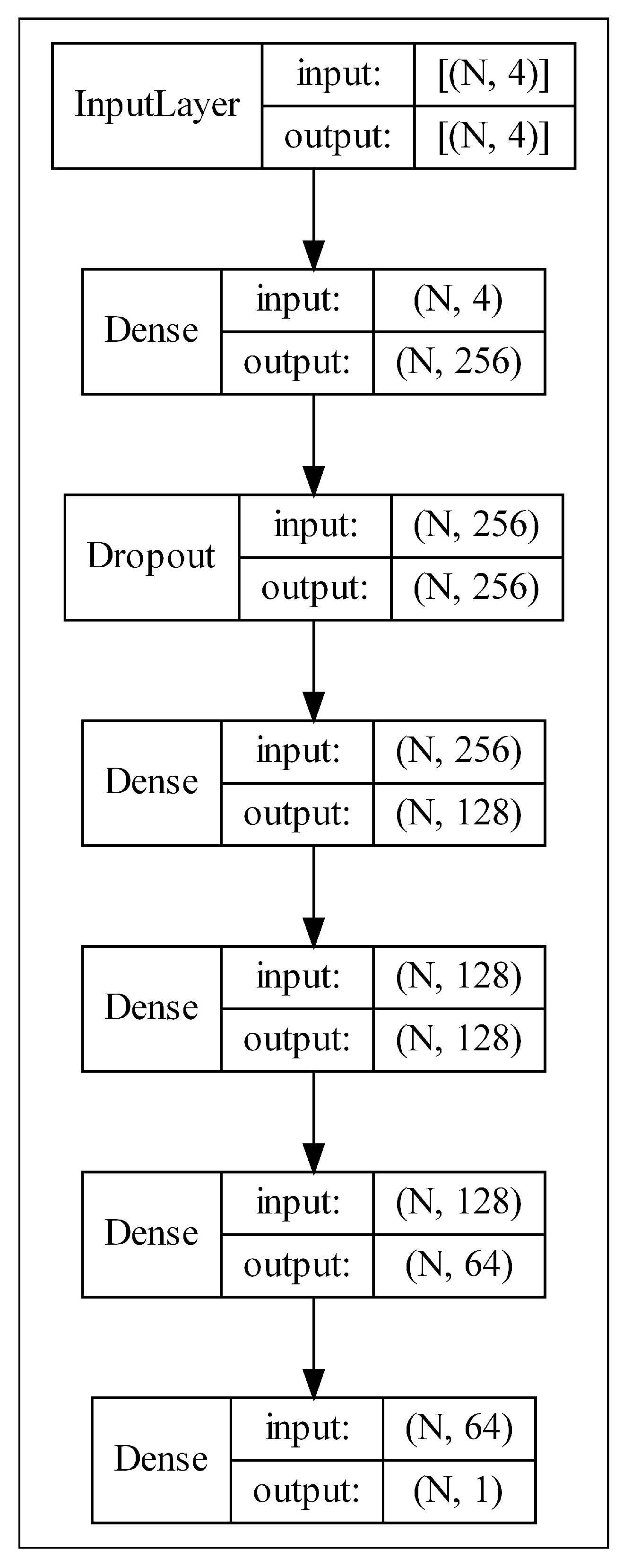
3.3.1. Multi-Layer Perceptron for Tabular Data

The simplest form of a deep learning model is a multi-layer perceptron (MLP). In such a network, each neuron is densely connected with the other neurons in the previous layer. The first building block in predicting rental prices is creating an MLP capable of handling the four structured features. As mentioned previously, it is challenging to determine an architecture that could perform close to the random forest. We performed hyperparameters tuning of our model using a random search method, and the optimal model is depicted in Figure 6. The tabular model significantly improved when using a hyperbolic tangent activation function (tanh) in all the dense layers, as also supported by some evidence [37]. The hyperbolic tangent activation function drastically improved the performance when adding more layers and neurons compared to the rectified linear activation function (ReLU) or other common activation functions. Moreover, a dropout rate of 0.1 was applied before the second dense layer to tackle over-fitting.

The scales of tabular features, such as the size of the property and location (longitude and latitude), are different; hence, feature scaling is a helpful means of ensuring that the performance of our models is maximized. NNs, in particular, could benefit from this, as scaling can lead to numerical stability and faster network convergence [38]. In both cases of NNs and ML models, we standardized the tabular features by centering and scaling all the variables, which may have helped our models improve performance and converge faster.

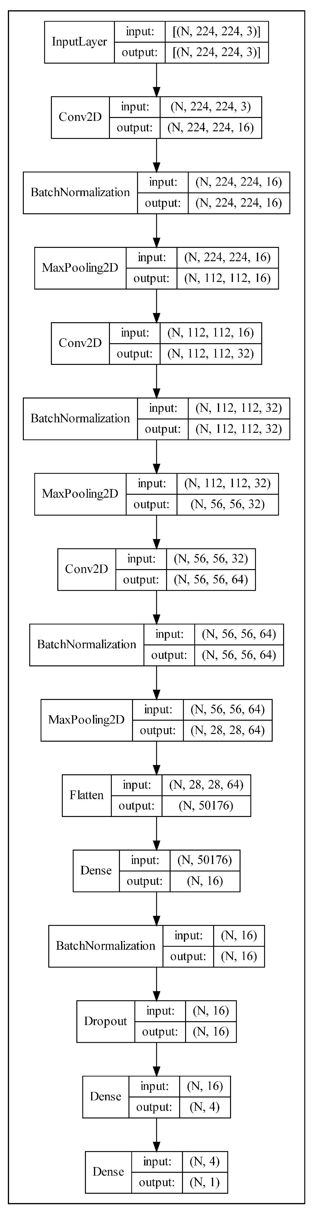
3.3.2. Feeding Multiple Images to NNs

As a single neural network can only process one image per property, we created a montage for each property containing the four relevant room types that resulted from stage 3 of image pre-processing. These categories include exterior images, bedroom, kitchen, and bathroom. Montages allow us to experiment with the position of the room type within the montage. Studies such as [13,14] believed that using organized or categorized room types where the position of the room type within the image was fixated is a valuable approach; in addition, [13] mentioned how they expected that ‘comparing rooms of the same type will give […] better results than comparing different room categories‘. We could put this claim to the test by first classifying the room types at the third stage of image processing and then generating two montages: a first montage that had all the room types in an organized manner (consistent positions across all properties) and a second montage where the room types had been shuffled and randomly positioned. Examples of both montages are shown in Figure 7, where, in the organized version, bathrooms are placed on the top left, living rooms on the top right, kitchens on the bottom left, and exterior images on the bottom right. We (and the researchers mentioned above) expected that the organized montages would outperform the randomly placed ones since we believed it would be easier for a model to cross-compare rooms of the same category, thereby improving its performance.

To elucidate the decision of creating montages and stage 3 of image pre-processing, we highlight how neural networks can take multiple images as inputs. To the best of our knowledge, there are three main methods for feeding multiple images for a single instance into a neural network:

(1) 

Feeding all images one by one and using the same property price as the outcome for each image. The least challenging approach is arguably passing each image from the listing one at a time through a neural network while directly setting the price as the outcome for each image. Such an approach replicates many current observations with only the image differing. There are two main limitations to this approach. The first is the possibility of such a model becoming confused and ineffective, as it is missing the context from the other images, which impacts its ability to build the bigger picture. For instance, it may be that the bathrooms are the main driver of the price among all properties. Such a model would not be able to identify that since it is not comparing a bathroom against bathrooms but a bathroom against every other kind of room. Conceivably, we could classify the room type and only feed images from a selected number of categories. Nonetheless, the problem of comparison against widely different room types remains. The second issue with this approach is that the number of images of a given listing may impact the overall model prediction, hence biasing the outcome. For instance, a listing with eight images will have eight replicated entries, and, as opposed to a listing with one image, it may mislead the regression model and dilute the results.

(2) 

Designingnindependent NNs for each of theximages whereby all the outputs fuse (e.g., concatenate) to predict a single price. The second option is to design n multiple NNs for the images, whereby n is either set as the maximum number of images found in all listings or fixed at the desired number. The former case is not feasible, as if x is the number of images for a given listing, and then for the difference $i\in \mathbb{Z}:x\le x+i\le n$, we would have to duplicate some of the x images or pass i as blank images (e.g., black or white images). Moreover, fixing the n could also work, and we could, for example, decide on setting $n=4$, assuming that we have four types of images; however, we would need to feed the same kind of room type into the branches to make sure the images are directly cross-comparable. In addition, another issue with designing multiple models is that it may be computationally inefficient. We also suspect that since training configurations such as the optimizer and learning rate are kept constant among all variations of NNs, it may be more difficult for a model with multiple n branches to converge than a simpler model with fewer branches; however, this remains merely a hypothesis, and its validation goes beyond the scope of this thesis. Finally, an advantage of using n models is the ability to experiment with different branches by temporarily disabling inputs (one or more room types) to understand better what image/room types have the most significant impact on the prices.

(3) 

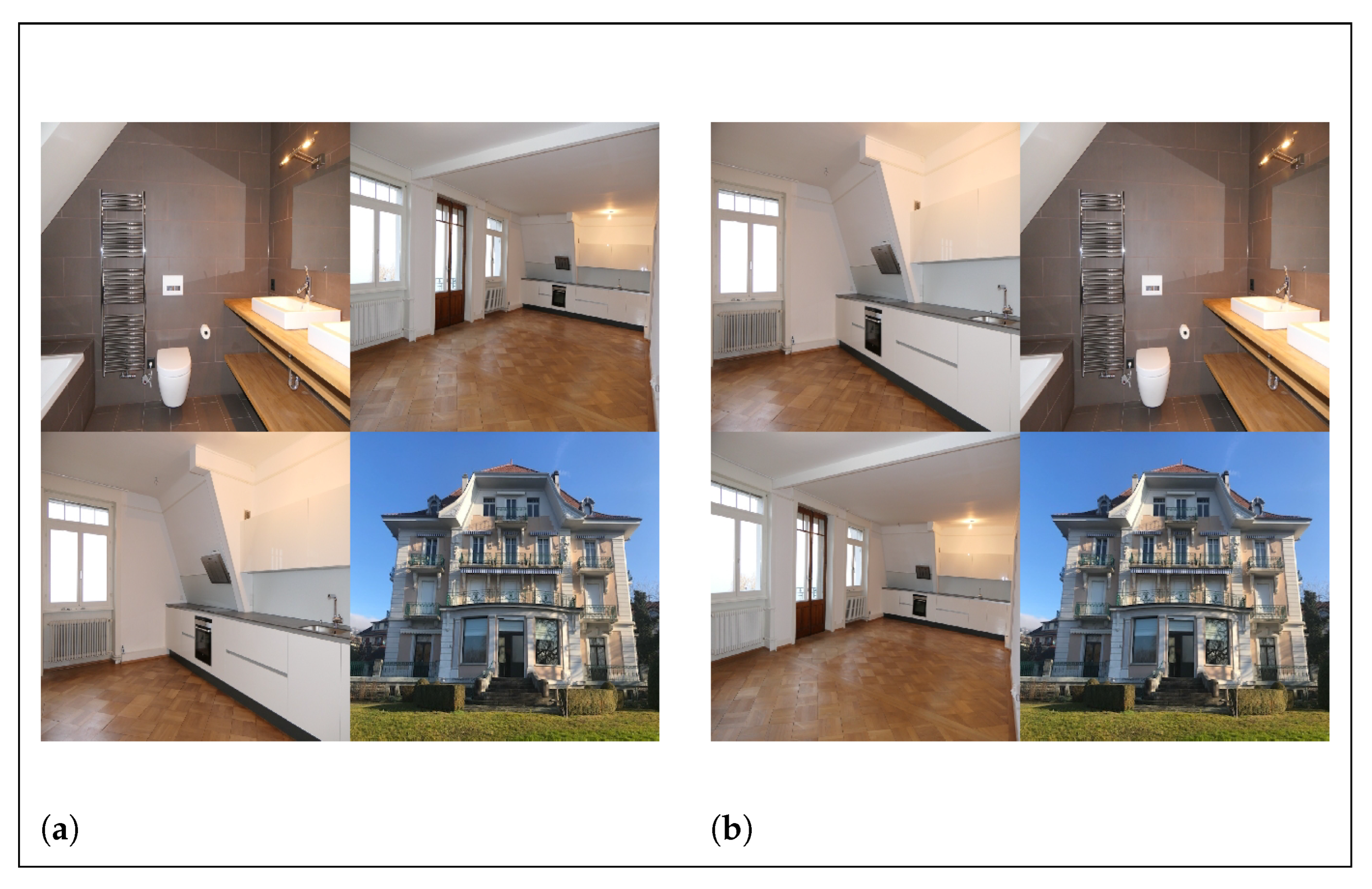
Create montages that combinenimages of the same listing into one image. One possible way of feeding multiple images into a neural network is combining them into a montage with the room types. The work that closely resembles our intended methodology is [8], where the authors used generated montages of wheat plots to predict numerical outcomes related to plants, such as their plant height. Creating a montage of room types over the two previous methods is preferred, as an initial model (not presented in this paper) revealed that this approach outperforms the technique where the images are fed into the network one at a time. Moreover, the montage approach has been favored due to the simplicity of this approach compared to designing n independent models, as well as the possibility of assessing organized as opposed to randomly designed montages.

3.3.3. Gradient Boosting Machine for Visual Data

Convolutional neural networks (CNNs) have shown remarkable performance on images and image recognition tasks [39]. CNN architecture is shown to perform better on image data than MLPs [40], since the former one uses a significantly less number of parameters. Further, using receptive fields in CNNs allows for identifying the same pattern at various locations of an image, while MLPs only recognize such patterns at a specific fixed area of the image. This made CNNs ideal both for identifying irrelevant classes as well as extracting visual cues from (i) interior and exterior images of properties and (ii) satellite images.

We found a single architecture to work well for both types of images. This final architecture of the image model is shown in Figure 8. We briefly explored the use of transfer learning for our regression task using various models [41,42,43,44], but as we did not see immediate improvements, we decided not to proceed further with this technique. For the optimizer, throughout all experiments, we set it to AdaMax (an extension to the adaptive movement estimation optimization algorithm) [45], with a learning rate of 0.0015, as we found this setting to perform better than other optimizers. Additionally, as we observed that the model optimizers with images converge slower than the tabular ones, we set a higher number of epochs for training and decided to use early stopping. The maximum number of training epochs was set at 350, with the early stopping of 25 epochs.

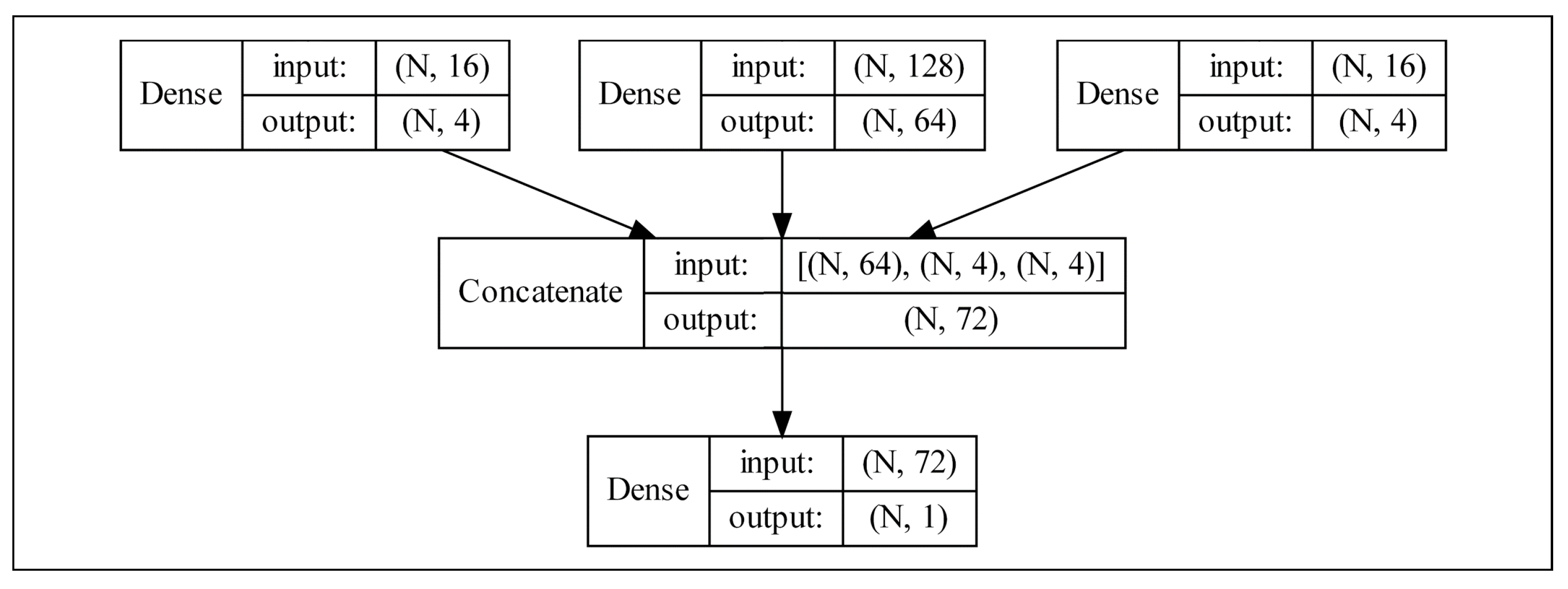
3.4. Multi-Modal Learning

ANNs can be aggregated into a single larger model to utilize the best features captured by each branch. This novel approach adds up to the three different kinds of inputs. Instead of making the prediction using one neuron in the last dense layer, the outputs are concatenated into one tensor, from which we then make a log price prediction. Figure 9 illustrates the top layers of the multi-modal network. This network automatically finds the best combination between the tabular features, property images, and satellite images without the need for human interference, much like a renter who considers all the factors together before making a decision.

Designing the network in such a way allows for experimentation. Simply disabling one of the input branches can reveal its effect on the overall performance. Additionally, it seems helpful to note that this network could have been designed differently if our choice of feeding property montages was instead to add a separate image of each room type as an input (see item 2 from Section 3.3.2), consequently resulting in a network with six branches (four-room types + tabular + satellite) instead of the current three. Such an approach would have increased the complexity of the task and possibly challenged the convergence of the model; however, it would have also allowed us to observe the exact room type, which, in combination with other factors, would improve or worsen the performance.

3.4.1. Ablation Study

Neural networks are capable of understanding complex relationships, which in turn helps them become powerful predictive tools, and yet, the inner workings of the model itself can often be challenging to interpret and, in turn, validate. As a part of our ablation studies [46], the architecture of the MLP and CNNs was always kept constant and only the image inputs were modified. For instance, in one scenario, a neural network was trained on the tabular feature and the organized property montages (NN T+OPI). In contrast, considering another scenario, a second neural network with the same architecture received the tabular features and randomly placed property images as the image input instead (NN T+RPI).

Such an ablation technique can be extended to understand the influence of the property images by comparing the results from a model estimating properties’ prices using tabular features and the corresponding real estate images (SRED) against another model with the same structure. However, instead of training with property images, the latter model is exposed to cat images combined with the tabular features. We do not expect such a model to perform better than a model that only uses tabular features, as there is no relationship between a cat image and a property’s rental price. In short, the cat images can validate the results from our modeling process. The cat image dataset was introduced by [47], where the authors studied the detection of cat heads.

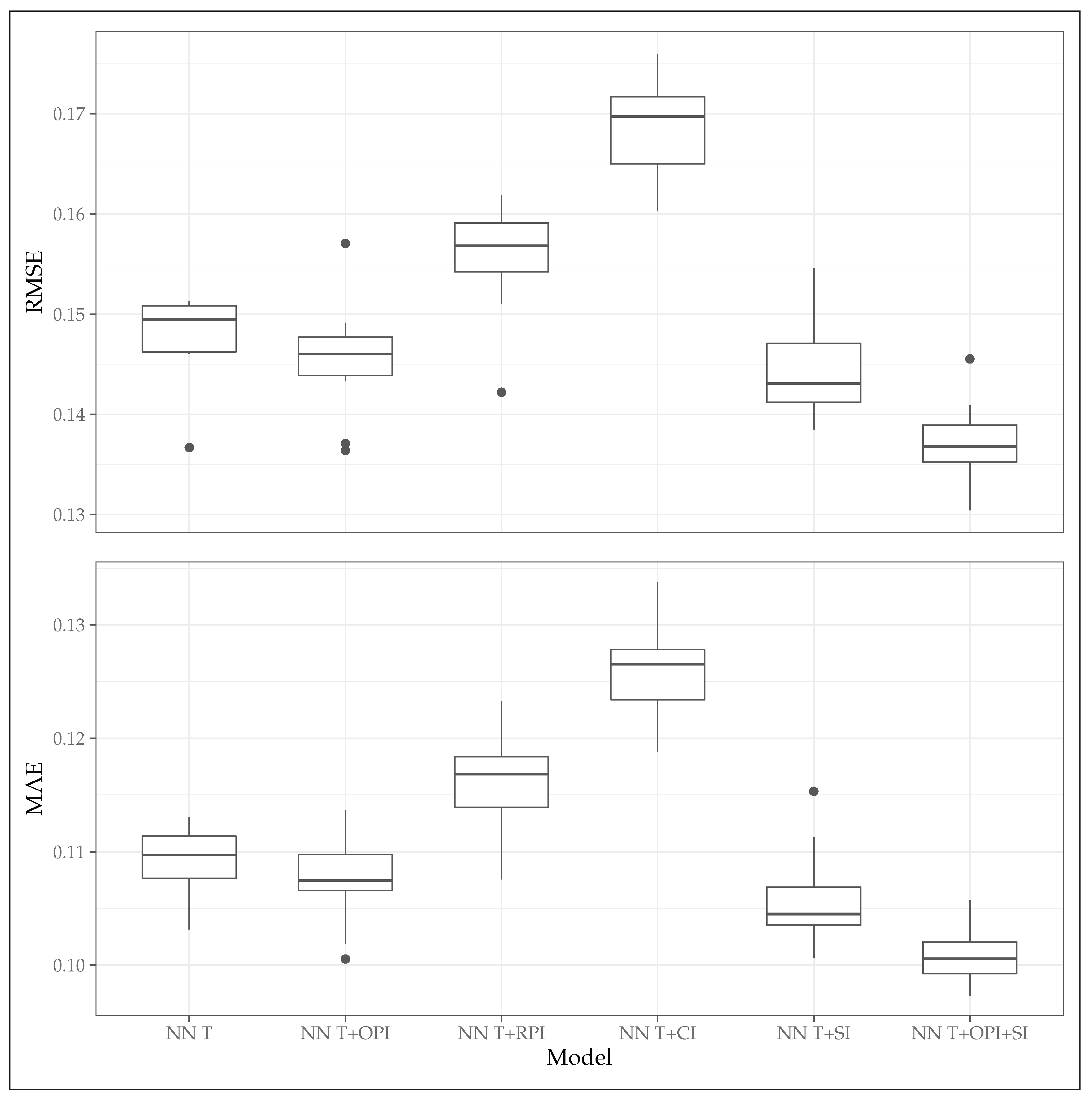
3.4.2. Performance Validation

In the ablation study for the first part of our research question, the choice of the hold-out set may influence the performance of various neural networks and lead to over-fitting, and to tackle this, we chose to cross-validate the results with ten folds. The SRED dataset was divided into ten folds, whereby NNs were trained on nine folds while validating the performance on the 10th fold. We repeated this process for every fold, where one of the previous training folds was taken as the new validation set while the old validation set joined the training data. Such an approach allowed us to treat each fold similarly to the unseen real-world data, and averaging the performance from each fold reassured us that the results were not dependent and unique to a single chosen fold. To answer the second part of our research question on comparing the performance of the final NNs with ML models, we trained all the models on 90% of the SRED listings and evaluated them on the remaining 10% of the data.

4. Results and Discussion

The results of 10-fold cross-validation for all the neural networks are depicted in

Table 4. Cross-validated performances on 10 folds.

Model	RMSE		MAE		${\mathrm{R}}^2$
	Mean	Median	Mean	Median	Mean	Median
NN T *	0.148	0.149	0.109	0.110	0.744	0.741
NN T+OPI †	0.146	0.146	0.107	0.107	0.752	0.757
NN T+RPI ‡	0.156	0.157	0.116	0.117	0.716	0.708
NN T+CI §	0.168	0.170	0.126	0.127	0.668	0.668
NN T+SI ††	0.144	0.143	0.106	0.105	0.756	0.754
NN T+OPI+SI ‡‡	0.137	0.137	0.101	0.101	0.779	0.776

Remarks: The best results are highlighted in bold. * Tabular features. ^† Tabular features and organized property images (interior and exterior). ^‡ Tabular features and randomly placed property images (interior and exterior). ^§ Tabular features and cat images. ^†† Tabular features and satellite images. ^‡‡ Tabular features and organized property and satellite images.

. The neural network that includes all three kinds of input (NN T+OPI+SI) reached the highest performance, exceeding the results of adding tabular data or image inputs separately to the models. Moreover, the boxplots of each fold in Figure 10 illustrate that when considering MAE and RMSE as evaluation metrics, the NN T+OPI+SI model globally performs better than the other NNs. The results showcase that tabular information and property-related images may contain relevant complementary information. Access to all input types allows our neural network to understand the context of the predictors and, in turn, build a more holistic understanding of how prices are estimated. The performance improvements which organized property montages offer (NN T+OPI) compared to randomly placing the room types (NN T+RPI) further highlight the importance of suitable pre-processing. Likewise, when using cat images to control the coherence and validity of these results (NN T+CI), the performance drastically worsens, which we believe to be caused by difficulty in model convergence, a performance worse than the one produced by the tabular model alone. The last two findings further support that the results obtained for NN T+OPI+SI are well grounded and that the correct pre-processing of images is required for performance improvements. The overall results indicate the power of deep learning models in complex environments where multiple variables and features may otherwise go unexplored.

Table 5. Single test set performances of NNs and ML models.

Model	RMSE		MAE		${\mathrm{R}}^2$
	Train	Test	Train	Test	Train	Test
LR T a	0.228	0.221	0.163	0.159	0.391	0.422
RF T b	0.065	0.144	0.047	0.105	0.955	0.753
GBM T c	0.100	0.139	0.076	0.103	0.884	0.770
XGB T d	0.026	0.137	0.017	0.099	0.993	0.775
NN T e	0.136	0.149	0.102	0.113	0.789	0.736
NN T+OPI+SI f	0.044	0.136	0.034	0.101	0.985	0.783

Remarks: The best results are highlighted in bold. ^a Linear regression with tabular features. ^b Random forest with tabular features. ^c gradient boosting machines with tabular features. ^d eXtreme gradient boosting with tabular features. ^e Neural network with tabular features. ^f Neural network with tabular features and property and satellite images.

demonstrates the results from comparing all the models on a single test set. These results reveal that the performance of linear regression is significantly worse than other models, yet it might still be used for commercial applications. On the contrary, when comparing the performance of neural networks against the ML models, NN T with only tabular features performs worse than all the ML models trained solely on tabular data. However, with the addition of property and satellite images, neural networks outperform all ML techniques when considering RMSE and ${\mathrm{R}}^2$ as primary metrics. The only model that outperforms NN T+OPI+SI in terms of MAE is XGB T.

Given the superior performance of random forest on the structure features, it can also be applied directly to the images; however, treating such a high-dimensional image directly with random forests may not be optimal [48]. Additionally, in a multi-modal setting, assigning the same importance to the structured features as the high number of pixels was challenging. As an alternative approach, neural networks could have served as feature extractors whereby their output became input to random forest [18,49]. Nonetheless, we believe that attaining high performance in this technique can be more complex and may require more feature engineering.

The superiority of multi-input networks in evaluation metrics is significant, yet it is also essential to consider the objective of the modeling task. Some applications require a high degree of interpretation and understanding of the contribution of the explanatory variables. Hence why linear regressions, despite their inferior performance in general, are still more frequently used than sophisticated machine learning models. Neural networks are more complex and generally less interpretable than many machine learning models. Despite dedicated methods such as regression activation maps [50], which can create heatmaps for neural networks and visualize the pixel derivations by convolutional layers, the complex relationship between multiple inputs remains largely unknown.

Conversely to a neural network, a random forest has some degree of interpretability through its variable importance capability. Although variable importance—a permutation-based technique—is often useful to interpret, extreme care is needed when employing it. There is some degree of multi-collinearity between variables, such as living space, rooms, and the number of bathrooms, which could produce misleading explanations when interpreting the role of the tabular variables. The importance of interpretation in the domain where such technologies are needed may be consequential in the commercial adoption of neural networks. The magnitude of improvement may not justify the additional complexity introduced by black-box approaches.

5. Conclusions

This paper explores the role of multi-modal learning in real estate rental estimations. The primary objective is to assess whether models that better utilize existing non-structured information, such as a property’s advertised photos and satellite images, can outperform hedonic pricing models. The results of our experiments on our novel dataset SRED reveal that visual data improve rental estimations and that, in particular, neural networks outperform ML models built only on tabular information. As a further contribution, we show that the performance of our model improves with the addition of each new source of visual information.

Regarding the choice of architecture for our final neural network, our architecture is only one of the many possible architectures. We are not concerned with the magnitude of improvement brought forward by the use of images. Instead, we aim to show that neural networks can derive intricate patterns and realize their value, similarly to humans. We believe that more optimal architectures could give rise to more drastic improvements; however, our results prove that contextual improvements through property-related images are possible primarily due to advancements in deep learning.

Finally, we propose a few ideas for future work on how to explore the value of multi-modal learning in a real estate contexts:

• Additional input data, such as the advertisement description—another form of unstructured data—may benefit rental estimations. Two examples of applications may be in the forms of the information extraction (IE) of relevant features, where those features exist in an unstructured form, or providing all the descriptions as a new branch to NN T+OPI+SI without any intermediate feature extraction.
• Instead of one montage of property images with the chosen room types, it is possible to create a branch for each room type, allowing for ablation studies whereby branches are added to or removed from the model.
• It would be beneficial to perform a similar study on the sales prices and observe similarities and differences with the rental estimations. Such an experiment can be carried out either with the sales data gathered by us (not presented in this paper) or through an external dataset.
• Our dataset is based on the Swiss real estate market. However, further investigation is needed to know whether our findings can extend to other countries and markets.

References

- Radford, A.; Kim, J.W.; Hallacy, C.; Ramesh, A.; Goh, G.; Agarwal, S.; Sastry, G.; Askell, A.; Mishkin, P.; Clark, J.; et al. Learning Transferable Visual Models from Natural Language Supervision. In Proceedings of the 38th International Conference on Machine Learning, ICML 2021, Virtual Event, 18–24 July 2021; Meila, M., Zhang, T., Eds.; PMLR: Groveland, CA, USA, 2021; Volume 139, pp. 8748–8763. [Google Scholar]
- Ofli, F.; Alam, F.; Imran, M. Analysis of Social Media Data using Multimodal Deep Learning for Disaster Response. arXiv 2020, arXiv:2004.11838. [Google Scholar]
- Litjens, G.; Kooi, T.; Bejnordi, B.E.; Setio, A.A.A.; Ciompi, F.; Ghafoorian, M.; van der Laak, J.A.; van Ginneken, B.; Sánchez, C.I. A survey on deep learning in medical image analysis. Med. Image Anal. 2017, 42, 60–88. [Google Scholar] [CrossRef] [PubMed]
- Baltrusaitis, T.; Ahuja, C.; Morency, L.P. Multimodal Machine Learning: A Survey and Taxonomy. IEEE Trans. Pattern Anal. Mach. Intell. 2019, 41, 423–443. [Google Scholar] [CrossRef] [PubMed]
- Sun, S. A survey of multi-view machine learning. Neural Comput. Appl. 2013, 23, 2031–2038. [Google Scholar] [CrossRef]
- Li, Y.; Yang, M.; Zhang, Z. A Survey of Multi-View Representation Learning. IEEE Trans. Knowl. Data Eng. 2019, 31, 1863–1883. [Google Scholar] [CrossRef]
- Chollet, F. Deep Learning with Python; Manning Publications Co.: Shelter Island, NY, USA, 2017; Chapter 7; pp. 234–240. [Google Scholar]
- Apolo-Apolo, O.E.; Pérez-Ruiz, M.; Martínez-Guanter, J.; Egea, G. A mixed data-based deep neural network to estimate leaf area index in wheat breeding trials. Agronomy 2020, 10, 175. [Google Scholar] [CrossRef]
- Chau, K.; Chin, T.L. A Critical Review of Literature on the Hedonic Price Model. Int. J. Hous. Sci. Its Appl. 2003, 2, 145–165. [Google Scholar]
- Bourassa, S.C.; Cantoni, E.; Hoesli, M. Predicting house prices with spatial dependence: A comparison of alternative methods. J. Real Estate Res. 2010, 32, 139–159. [Google Scholar] [CrossRef]
- Law, S.; Paige, B.; Russell, C. Take a look around: Using street view and satellite images to estimate house prices. ACM Trans. Intell. Syst. Technol. 2019, 10, 1–19. [Google Scholar] [CrossRef]
- Wittowsky, D.; Hoekveld, J.; Welsch, J.; Steier, M. Residential housing prices: Impact of housing characteristics, accessibility and neighbouring apartments—A case study of Dortmund, Germany. Urban Plan. Transp. Res. 2020, 8, 44–70. [Google Scholar] [CrossRef]
- Poursaeed, O.; Matera, T.; Belongie, S. Vision-based real estate price estimation. Mach. Vis. Appl. 2018, 29, 667–676. [Google Scholar] [CrossRef]
- Ahmed, E.H.; Moustafa, M. House price estimation from visual and textual features. In Proceedings of the 8th International Joint Conference on Computational Intelligence—NCTA, Porto, Portugal, 9–11 November 2016; Volume 3, pp. 62–68. [Google Scholar] [CrossRef]
- Lee, C.; Park, K.H. Using photographs and metadata to estimate house prices in South Korea. Data Technol. Appl. 2020, 55, 280–292. [Google Scholar] [CrossRef]
- Zhao, Y.; Chetty, G.; Tran, D. Deep Learning with XGBoost for Real Estate Appraisal. In Proceedings of the 2019 IEEE Symposium Series on Computational Intelligence, SSCI 2019, Xiamen, China, 6–9 December 2019; Institute of Electrical and Electronics Engineers Inc.: Piscataway, NJ, USA, 2019; pp. 1396–1401. [Google Scholar] [CrossRef]
- Murray, N.; Marchesotti, L.; Perronnin, F. AVA: A large-scale database for aesthetic visual analysis. In Proceedings of the IEEE Computer Society Conference on Computer Vision and Pattern Recognition, Providence, RI, USA, 16–21 June 2012; pp. 2408–2415. [Google Scholar] [CrossRef]
- Kucklick, J.P.; Oliver, M.; Str, W. A Comparison of Multi-View Learning Strategies for Satellite Image-Based Real Estate Appraisal. arXiv 2021, arXiv:2105.04984. [Google Scholar]
- Bency, A.J.; Rallapalli, S.; Ganti, R.K.; Srivatsa, M.; Manjunath, B.S. Beyond spatial auto-regressive models: Predicting housing prices with satellite imagery. In Proceedings of the 2017 IEEE Winter Conference on Applications of Computer Vision, WACV 2017, Santa Rosa, CA, USA, 24–31 March 2017; pp. 320–329. [Google Scholar] [CrossRef]
- Breiman, L. Random Forests. Mach. Learn. 2001, 45, 5–32. [Google Scholar] [CrossRef]
- Friedman, J.H. Greedy function approximation: A gradient boosting machine. Ann. Stat. 2001, 29, 1189–1232. [Google Scholar] [CrossRef]
- Chen, T.; Guestrin, C. XGBoost: A scalable tree boosting system. In Proceedings of the ACM SIGKDD International Conference on Knowledge Discovery and Data Mining, San Francisco, CA, USA, 13–17 August 2016; pp. 785–794. [Google Scholar] [CrossRef]
- Bentéjac, C.; Csörgo, A.; Martínez-Muñoz, G. A comparative analysis of gradient boosting algorithms. Artif. Intell. Rev. 2021, 54, 1937–1967. [Google Scholar] [CrossRef]
- Nica, I.; Alexandru, D.B.; Crăciunescu, S.L.P.; Ionescu, Ș. Automated Valuation Modelling: Analysing Mortgage Behavioural Life Profile Models Using Machine Learning Techniques. Sustainability 2021, 13, 5162. [Google Scholar] [CrossRef]
- R Core Team. R: A Language and Environment for Statistical Computing; R Foundation for Statistical Computing: Vienna, Austria, 2022. [Google Scholar]
- Kuhn, M. Caret: Classification and Regression Training; R Package Version 6.0-92; R Foundation for Statistical Computing: Vienna, Austria, 2022. [Google Scholar]
- Liaw, A.; Wiener, M. Classification and Regression by randomForest. R News 2002, 2, 18–22. [Google Scholar]
- LeDell, E.; Gill, N.; Aiello, S.; Fu, A.; Candel, A.; Click, C.; Kraljevic, T.; Nykodym, T.; Aboyoun, P.; Kurka, M.; et al. h2o: R Interface for the ‘H2O’ Scalable Machine Learning Platform; R Package Version 3.36.1.2; R Foundation for Statistical Computing: Vienna, Austria, 2022. [Google Scholar]
- Chen, T.; He, T.; Benesty, M.; Khotilovich, V.; Tang, Y.; Cho, H.; Chen, K.; Mitchell, R.; Cano, I.; Zhou, T.; et al. xgboost: Extreme Gradient Boosting; R Package Version 1.6.0.1; R Foundation for Statistical Computing: Vienna, Austria, 2022. [Google Scholar]
- Abiodun, O.I.; Jantan, A.; Omolara, A.E.; Dada, K.V.; Mohamed, N.A.; Arshad, H. State-of-the-art in artificial neural network applications: A survey. Heliyon 2018, 4, e00938. [Google Scholar] [CrossRef]
- Gorishniy, Y.; Rubachev, I.; Khrulkov, V.; Babenko, A. Revisiting Deep Learning Models for Tabular Data. In Proceedings of the Advances in Neural Information Processing Systems, Virtual, 14 December 2021; Ranzato, M., Beygelzimer, A., Dauphin, Y., Liang, P., Vaughan, J.W., Eds.; Curran Associates, Inc.: Red Hook, NY, USA, 2021; Volume 34, pp. 18932–18943. [Google Scholar]
- Voulodimos, A.; Doulamis, N.; Doulamis, A.; Protopapadakis, E.; Andina, D. Deep Learning for Computer Vision: A Brief Review. Intell. Neurosci. 2018, 2018, 7068349. [Google Scholar] [CrossRef]
- Otter, D.W.; Medina, J.R.; Kalita, J.K. A Survey of the Usages of Deep Learning for Natural Language Processing. IEEE Trans. Neural Netw. Learn. Syst. 2021, 32, 604–624. [Google Scholar] [CrossRef] [PubMed]
- Allaire, J.; Chollet, F. keras: R Interface to ‘Keras’; R Package Version 2.9.0; R Foundation for Statistical Computing: Vienna, Austria, 2022. [Google Scholar]
- Allaire, J.; Tang, Y. tensorflow: R Interface to ‘TensorFlow’; R Package Version 2.9.0; R Foundation for Statistical Computing: Vienna, Austria, 2022. [Google Scholar]
- O’Mahony, N.; Campbell, S.; Carvalho, A.; Harapanahalli, S.; Hernandez, G.V.; Krpalkova, L.; Riordan, D.; Walsh, J. Deep learning vs. traditional computer vision. In Proceedings of the Science and Information Conference, Tokyo, Japan, 16–19 March 2019; Springer: Berlin/Heidelberg, Germany, 2019; pp. 128–144. [Google Scholar]
- Feng, J.; Lu, S. Performance Analysis of Various Activation Functions in Artificial Neural Networks. J. Phys. Conf. Ser. 2019, 1237, 111–122. [Google Scholar] [CrossRef]
- LeCun, Y.A.; Bottou, L.; Orr, G.B.; Müller, K.R. Efficient BackProp. In Neural Networks: Tricks of the Trade, 2nd ed.; Montavon, G., Orr, G.B., Müller, K.R., Eds.; Springer: Berlin/Heidelberg, Germany, 2012; pp. 9–48. [Google Scholar] [CrossRef]
- Rawat, W.; Wang, Z. Deep Convolutional Neural Networks for Image Classification: A Comprehensive Review. Neural Comput. 2017, 29, 2352–2449. [Google Scholar] [CrossRef] [PubMed]
- Géron, A. Hands-On Machine Learning with Scikit-Learn, Keras, and TensorFlow: Concepts, Tools, and Techniques to Build Intelligent Systems; O’Reilly Media, Inc.: Sebastopol, CA, USA, 2019. [Google Scholar]
- Szegedy, C.; Ioffe, S.; Vanhoucke, V.; Alemi, A.A. Inception-v4, inception-ResNet and the impact of residual connections on learning. In Proceedings of the 31st AAAI Conference on Artificial Intelligence, AAAI 2017, San Francisco, CA, USA, 4–9 February 2017; pp. 4278–4284. [Google Scholar]
- Chollet, F. Xception: Deep learning with depthwise separable convolutions. In Proceedings of the 30th IEEE Conference on Computer Vision and Pattern Recognition, CVPR 2017, Honolulu, HI, USA, 21–26 July 2017; pp. 1800–1807. [Google Scholar] [CrossRef]
- He, K.; Zhang, X.; Ren, S.; Sun, J. Deep Residual Learning for Image Recognition. In Proceedings of the IEEE Conference on Computer Vision and Pattern Recognition, Las Vegas, NV, USA, 27–30 June 2016; pp. 770–778. [Google Scholar] [CrossRef]
- Sandler, M.; Howard, A.; Zhu, M.; Zhmoginov, A.; Chen, L.C. MobileNetV2: Inverted Residuals and Linear Bottlenecks. In Proceedings of the IEEE Computer Society Conference on Computer Vision and Pattern Recognition, Salt Lake City, UT, USA, 18–22 June 2018; pp. 4510–4520. [Google Scholar] [CrossRef]
- Kingma, D.P.; Ba, J. Adam: A Method for Stochastic Optimization. In Proceedings of the 3rd International Conference on Learning Representations, Conference Track Proceedings, ICLR 2015, San Diego, CA, USA, 7–9 May 2015. [Google Scholar]
- Meyes, R.; Lu, M.; de Puiseau, C.W.; Meisen, T. Ablation Studies in Artificial Neural Networks. arXiv 2019, arXiv:1901.08644. [Google Scholar]
- Zhang, W.; Sun, J.; Tang, X.; Zhang, W.; Sun, J.; Tang, X. Cat Head Detection— How to Effectively Exploit Shape and Texture Features. In Proceedings of the European Conference on Computer Vision, Marseille, France, 12–18 October 2008; Forsyth, D., Torr, P., Zisserman, A., Eds.; Springer: Berlin/Heidelberg, Germany, 2008; pp. 802–816. [Google Scholar]
- Liu, T.; Abd-Elrahman, A.; Jon, M.; Wilhelm, V. Comparing Fully Convolutional Networks, Random Forest, Support Vector Machine, and Patch-based Deep Convolutional Neural Networks for Object-based Wetland Mapping using Images from small Unmanned Aircraft System. GIScience Remote Sens. 2018, 55, 243–264. [Google Scholar] [CrossRef]
- Gupta, S.; Arbeláez, P.; Malik, J. Perceptual Organization and Recognition of Indoor Scenes from RGB-D Images. In Proceedings of the 2013 IEEE Conference on Computer Vision and Pattern Recognition, Portland, OR, USA, 23–28 June 2013; pp. 564–571. [Google Scholar] [CrossRef]
- Wang, Z.; Yang, J. Diabetic Retinopathy Detection via Deep Convolutional Networks for Discriminative Localization and Visual Explanation. In Proceedings of the 2018 International Conference on Virtual Reality and Visualization (ICVRV), Qingdao, China, 22–24 October 2018. [Google Scholar]