Article

Multimodal Emotional Classification Based on Meaningful Learning

Laboratory of Computer Science, Signals, Automation and Cognitivism (LISAC), Department of Computer Science, Faculty of Sciences Dhar El Mahraz, Sidi Mohamed Ben Abdellah University, Fez 30000, Morocco
*
Author to whom correspondence should be addressed.
Big Data Cogn. Comput. 2022, 6(3), 95; https://doi.org/10.3390/bdcc6030095
Submission received: 28 July 2022 / Revised: 26 August 2022 / Accepted: 31 August 2022 / Published: 8 September 2022

Abstract

:
Emotion recognition has become one of the most researched subjects in the scientific community, especially in the human–computer interface field. Decades of scientific research have been conducted on unimodal emotion analysis, whereas recent contributions concentrate on multimodal emotion recognition. These efforts have achieved great success in terms of accuracy in diverse areas of Deep Learning applications. To achieve better performance for multimodal emotion recognition systems, we exploit Meaningful Neural Network Effectiveness to enable emotion prediction during a conversation. Using the text and the audio modalities, we proposed feature extraction methods based on Deep Learning. Then, the bimodal modality that is created following the fusion of the text and audio features is used. The feature vectors from these three modalities are assigned to feed a Meaningful Neural Network to separately learn each characteristic. Its architecture consists of a set of neurons for each component of the input vector before combining them all together in the last layer. Our model was evaluated on a multimodal and multiparty dataset for emotion recognition in conversation MELD. The proposed approach reached an accuracy of 86.69%, which significantly outperforms all current multimodal systems. To sum up, several evaluation techniques applied to our work demonstrate the robustness and superiority of our model over other state-of-the-art MELD models.

1. Introduction

Emotions can be defined as a conscious mental reaction, usually directed towards a specific object, and accompanied by dynamic physiological changes that occur non-verbally [1], allowing the identification of emotions as a very complicated task.
The process of recognizing emotions is dynamic and focuses on the individual’s emotional state; thus, each person has a particular set of feelings that correlate to their actions [2]. Humans generally express their emotions in a variety of ways. The right understanding of these emotions is crucial for successful communication. However, recognizing emotions in daily life is crucial for social interaction, and emotions are a major factor in how people act [3]. Emotions are manifested through voice intonation, gestures as well as body posture, speech, and most often through facial expressions, which account for 55% of nonverbal communication. However, a single modality is unable to quickly assess the emotion of the person [4]. We cannot decide the emotion of a person by examining a particular entity or occurrence in front of our eyes [5]. This is one of the reasons why emotion recognition should be treated as a multimodal problem.
There is an integration of many approaches and strategies to achieve the goal of the study. Most of them use big data techniques [6], semantic principles [7], and deep learning [8].
A variety of various solutions to a range of multimodal sequential challenges have been developed as a result of the rapid development of DL architectures over the past decade.
The literature has demonstrated numerous methods for producing robust multimodal features using DL. from a single model of expression, such as facial expression [9], speech [10], text [11], EEG signal [12], etc. Since approaches based on DL have proven to be effective in learning and generalizing data with high dimensional feature spaces such as images, several emotion datasets have also produced promising results from comparable attempts to capture the intricate feature space of emotional data, such as MELD [13,14], IEMOCAP [15], MOSI [16], etc. Unfortunately, human emotions in real life are often expressed by a complex combination of several expression models.
So, much information is lost by employing unimodal analysis. To address this problem, the use of approaches based on DL for MER has received much research in recent years. Choi et al. [17] who utilized a novel approach to learning about the hidden representations between text and speech data using convolutional attention networks proposed end-to-end MER with auditory and visual modalities. The speech and the visual networks were built by Tzirakiz et al. [18] using a convolutional neural network (CNN) and deep residual network, respectively. To obtain the contextual information, the outputs of the two networks were combined as the input of a two-layer Long Short-Term Memory (LSTM). By feeding these features to a multiple kernel learning classifier, Poria et al. [19] proposed a novel technique for extracting features from visual and textual modalities using deep convolutional neural networks.
Inspired by these methods, we invented this work that focuses on the MER. It proposes a new system based on supervised learning algorithms, using three modalities: the first one concerns the text modality, its feature vector is extracted with CNN and LSTM; the second one depends on the audio modality that we acquired using the OpenSmile tool. While the third modality is obtained through the fusion of the text and audio features into a single vector that will represent the bimodal modality. These modalities vectors will feed the MNN that we have used as a methodological invention in order to have better predictive results. The MER by a computer is considered as a technology in full development. These innovative applications concern several domains such as human–computer interaction. Maat and Pantic’s research [20], in which the authors created a system to support effective multimodal human–computer interaction, serves as an illustration of this field of study (AMM-HCI). The interaction is then modified to reflect the user’s actions and feelings in order to assist the user in his activity. A further application’s domain concerns the help of autistic children. In this study [21], the authors explored multimodal emotion and gaze recognition deficits in children with autism spectrum disorders. Another example in the MER domain concerns video games; Nemati et al. [22] proposed a hybrid data fusion method in latent space for MER. Furthermore, faced with the Corona pandemic, MER applications are developed. Prasad et al. [23] propose a system that analyzes feelings and emotions for effective human–machine interaction during the COVID-19 pandemic, etc.
The rest of this paper is structured as follows: In Section 2, we clarify the background and related works. In Section 3, we defined the materials and methods we used in our paper. Then, in Section 4, we describe each of the proposed methods and their steps. In Section 5, we present the results of the comparison between our approach and the existing work. Finally, a conclusion is given in Section 6.

2. Related Works

Numerous studies based on DL have been conducted to study MER systems, namely, Priyasad et al. [24], who present an approach based on DL to exploit and merge text and acoustic data for emotion classification. In order to extract acoustic features from raw audio, a SincNet layer, band-pass filtering, and neural network are used. The output of these band-pass filters is then applied to the input of the Deep Convolutional Neural Network (DCNN). For word processing, they use two branches: a DCNN and a bidirectional Recurrent Neural Network (RNN), followed by a parallel DCNN where cross-attention is introduced to infer correlations at the N-gram level. Their experimental results on the IEMOCAP dataset achieve a 3.5% improvement in weighted accuracy. Researchers have looked into many features of multimodal autonomous human emotion recognition in the actual world [25]. In particular, Support Vector Machine (SVM) is utilized to categorize each feature, and they subsequently suggest a cutting-edge decision-level fusion network to utilize these feature characteristics. Their network was tested using the EmotiW 2015 AFEW and SFEW datasets, and it shows good results on the testing sets. The audio/visual emotion challenge (AVEC) 2012 [26], which presented baseline models for concatenating the audio and visual features into a single feature vector and used support vector regression to predict the continuous affective values, was one of the major attempts to advance the state of the art in MER. Another study was conducted on the German language for the purpose of extracting the emotions from three modalities: visual, audio, and text by Cevher et al. [27]. For extracting face expressions and audio features, they used an off-the-shelf tool. Word2vec and Bidirectional LSTM (BiLSTM) are used to extract textual features. For the purpose of predicting emotions, Georgiou et al. [28] concatenated features from several modalities at various levels. They showed that their proposed fusion method achieves greater performance gains compared to other fusion approaches in the literature. To identify the emotions, Bahreini et al. [29] suggested combining auditory, textual, and facial information. They used CNN to extract features from speech, and ResNet 50 to extract features from visual frames. These two modalities are captured using two different pipelines, valence and arousal are then extracted using an LSTM-based fusion. Their research demonstrated that merging two distinct modalities into a multimodal approach increased the software’s accuracy and produced more reliable results. A method to combine speech textual content and voice tonality for identifying emotions in conversation was proposed by Poria et al. [13] Additionally, they offered their benchmark dataset for multi-party emotional conversations based on the Friend dataset. They used 1D CNN to extract textual utterance characteristics, and they computed audio utterance features using OpenSmile to extract vocal and prosodic features of the speech. Likewise, Slavova et al. [30] used textual and speech features for the purpose of extracting sound from human speech. CNN features are retrieved from a basic plain transcription of the speech, while speech features such as speech spectrum and Mel-frequency cepstral coefficients (MFCCs) are extracted from the audio stream. These two teams concentrated on the transcription of voice tone for emotion recognition. In a recent study [31], visual and textual signals were used in speech emotion recognition through a hybrid fusion technique known as a multimodal attention network (MMAN). They propose a brand-new multimodal focus mechanism called cLSTM-MMA, which selectively combines information and promotes attention across three modalities. Other unimodal subnetworks are fused with the cLSTM-MMA during late fusion. The tests show that textual and visual signals are quite helpful in identifying speech emotions. While having a significantly more condensed network topology, the suggested cLSTM-MMA alone is just as successful in terms of precision as other fusion approaches. For self-supervised learning (SSL), Siriwardhana et al. [31] investigated the use of the pretrained “BERT-like” architecture to represent both language and text modalities in order to identify the multimodal language emotions. They show that a basic fusion mechanism (Shallow-Fusion) strengthens sophisticated fusion mechanisms while simplifying the overall structure. In this work [32], the authors proposed a deep hierarchical architecture for modality fusion and applied it to the problem of sentiment analysis from the audio and text modalities. Their proposed method achieves state-of-the-art results in sentiment analysis on the MOSI database. In [17], the authors adopted an attention method to learn the multi-modal representation between speech and textual modalities and used different CNNs to extract the features from embedding word sequences and speech spectrograms. For the Audio-Visual Emotion Challenge (AVEC 2017), Huang et al. [33] proposed an automatic prediction of dimensional emotional state using a Long Short-Term Memory Recurrent Neural Network (LSTM-RNN) to train several feature modalities and concatenate various feature vectors. A conversational transformer network (CTNet) was suggested by another recent study [34] to describe the context- and speaker-sensitive dependencies in a conversation as well as the inter- and intra-modality interactions for multimodal features. The outcomes confirmed the viability of the suggested transformer fusion technique. In order to investigate the emotion representation of a query from word- and utterance-level views, Hui et al. [35] introduced a multi-view network (MVN). Their experimental findings on two datasets of conversations on public emotions demonstrate that their suggested model outperforms the leading-edge baselines. An innovative Transformers and Attention-based fusion technique was presented by the authors in [36] that combines multimodal self-supervised learning features based on text, audio, and visual input. The model is resilient and outperforms state-of-the-art models on four datasets, according to the evaluation research. Multimodal emotion identification based on audio, video, and text modalities was accomplished by Baijun et al. [37] using a transformer-based cross-modal fusion and the EmbraceNet architecture. On the MELD dataset, their experimental results show up to 65% accuracy.
Despite the improvements achieved by the researchers in the MER, we were able to use a classification network MNN, elaborated by us, which allows different modalities to be classified significantly. In fact, our network learns each vector’s component separately and applies a concatenation until the fusion layer, not like the other architectures that merge the modalities without taking into consideration the different components of the resulting vector for each one. So, the accuracy is raised with 21% as the rate.

3. Materials and Methods

3.1. Convolutional Neural Networks

In this part, we will focus on one of the most powerful algorithms of DL, the Convolutional Neural Network or CNN, which was first introduced in 1998 by Yann LeCun [38], CNNs are a sub-category of neural networks and are currently one of the most efficient image classification models allowing, in particular, the recognition of images by automatically attributing to each image provided as input, a label corresponding to its class.
Generally, the architecture of a CNN consists of convolution layers, pooling layers, plus layers of neurons that are fully connected in the form of a Multilayer Perceptron (MLP) called fully connected layers.
Moreover, CNNs are composed of two main parts as presented in Figure 1, which are: the hidden layer part, also called feature extraction, and the classification part.
In the hidden layers, the network performs a series of convolution and pooling operations during which features will be detected.
The convolution layer’s job is to examine the images that are provided as input and find the existence of a particular set of features. A set of feature maps is located in the output of this layer.
G ( m , n ) = ( f * h ) [ m , n ] = j k h [ j , k ] f [ m j , n k ]
The main difference between standard image processing algorithms and CNNs is that in the latter, the weights or values of the filters are learned by an optimization algorithm during the training phase. This allows convolutional neural networks to learn the specific filters for each task. After applying convolution operations on the input images, the results (feature maps) will go through a non-linear activation function; for example, the ReLu function, which replaces all the negative values received as inputs with zeros. The interest of these activation layers is to make the model non-linear and therefore more complex. The ReLu function can be calculated by the following formula:
f ( x ) = max ( 0 , x )
Then, the results will be transferred to the pooling layer that is used, on the one hand, to reduce the number of parameters by minimizing the size of the characteristic maps and, on the other hand, to introduce translational invariance into the model.
Let A = [ a i , j ] n * m be a matrix that represents a characteristic map of a specific region, and that will be presented to the pooling layer. The most commonly used pooling methods are the following:
  • Max pooling: replaces the input region with its maximum value.
    P ( A ) = max ( A ) = max ( a i , j | i 1 , , n , j 1 , , m )
  • Average pooling (weighted average pooling): pools the input region by taking its average or a weighted sum, which can be based on the distance from the region center.
    P ( A ) = 1 n m = i = 1 n j = 1 m a i , j
  • The Fully Connected (FC) layer, which is at the end of the CNN design and is fully connected to every output neuron, is used for classification. To classify the input image, the FC layer first applies a linear combination and then an activation function after receiving an input vector. In the end, it returns a vector of size d, where d is the number of classes and each component is the likelihood that the input image belongs to a particular class.

3.2. Long Short-Term Memory

Long short-term memory (LSTM) is an artificial recurrent neural network architecture, frequently used in natural language processing. The LSTM was initially proposed by S. Hochreiter et al. [39], then improved in the article of F. Gers et al. [40] The main idea of recurrent neural networks is to have the ability of keeping a state over a long period of time. Moreover, this is the goal of LSTM cells, which have an internal memory called cell. This last one allows a state to be maintained as long as necessary, and consists of a numerical value that the network can control according to the situation.
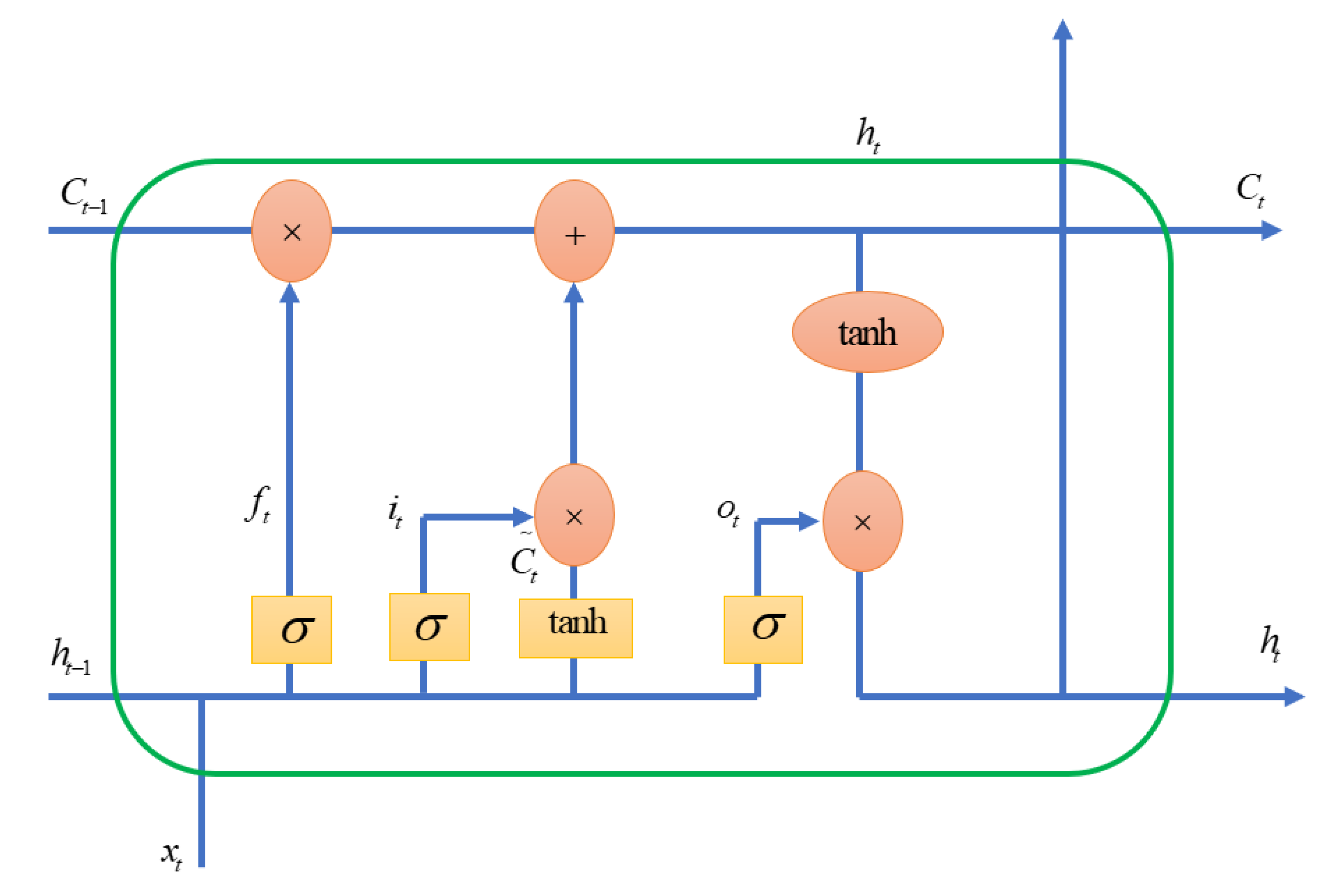
An LSTM’s overall operation can be divided into three steps:
  • Identifying pertinent information from the past, taken from the cell state through the forget gate;
  • Using the input gate to choose from the current input those items that will be important in the long term. The cell state, which serves as long-term memory, will be added to these;
  • Select the crucial short-term information from the newly created cell state and use the output gate to create the subsequent hidden state.
The LSTM defines a recurrence relation using an additional variable, which is the cell state c :
h t , c t = f ( x t , h t 1 , c t 1 )
The information transits from one cell to the next through two channels, h and c . At time t , these two channels are updated by the interaction between their previous values h t 1 , c t 1 and the current element of the sequence x t . Figure 2 shows the simplified diagram of an LSTM cell.
The equations governing the three control gates are therefore the following: they are the application of the weighted sum followed by the application of an activation function.
  • Forget gate:
    The forget gate determines what information must be remembered and what can be forgotten. Data derived from the current input x t and hidden state h t 1 are absorbed by the sigmoid function. The values that Sigmoid produces range from 0 to 1. It draws a conclusion regarding the necessity of the old output’s part (by giving the output closer to 1). The cell will eventually use this value of f t for point-by-point multiplication.
    f t = σ ( w f . [ h t 1 , x t ] + b f )
    t : timestep, f t : forget gate at t , x t : input, h t 1 : previous hidden state, w f : weight matrix between forget gate and input gate, b t : connection bias at t .
  • Input gate:
    Updates to the cell state are made by the input gate using the following operations. To begin with, the second sigmoid function receives the current state, x t , and the previously hidden information, h t 1 . The values are specified to range from 0 (important) to 1 (not important).
    The same data from the current state and concealed state will then be transferred through the tanh function. The network will be controlled by the tanh operator, which will produce a vector C t containing every conceivable value between −1 and 1. Point-by-point multiplication can be performed on the output values produced by the activation functions.
    i t = σ ( w i . [ h t 1 , x t ] + b i )
    C t = tanh ( w c . [ h t 1 , x t ] + b c )
    t : timestep, i t : input gate at t , x t : input, w i : weight matrix of sigmoid operator between input gate and output gate, b i : bias vector at t , C t : value generated by tanh, w c : weight matrix of tanh operator between cell state information and network output, b c : bias vector at t .
    The input gate and forget gate have provided the network with sufficient data. Making a decision and storing the data from the new state in the cell state come next. The forget vector f t multiplies the previous cell state C t 1 . Values will be removed from the cell state if the result is 0. The network then executes point-by-point addition on the output value of the input vector i t , which updates the cell state and gives the network a new cell state C t .
    C t = f t C t 1 + i t C t
    t : timestep, i t : input gate at t , C t : value generated by tanh, f t : forget gate at t, C t 1 : previous timestep.
  • Output gate:
    The value of the following hidden state is decided by the output gate. Information about prior inputs is contained in this state.
    First, the third sigmoid function receives the values of the current state and the prior concealed state. The tanh function is then applied to the new cell state that was created from the original cell state. These two results are multiplied one by one. The network determines which information the hidden state should carry based on the final value. For prediction, this hidden state is used.
    o t = σ ( w 0 . [ h t 1 , x t ] + b 0 )
    h t = o t tanh ( C t )
    t : timestep, o t : output gate at t , w 0 : weight matrix of output gate, b 0 : bias vector, h t : LSTM output.

3.3. The Meaningful Neural Network

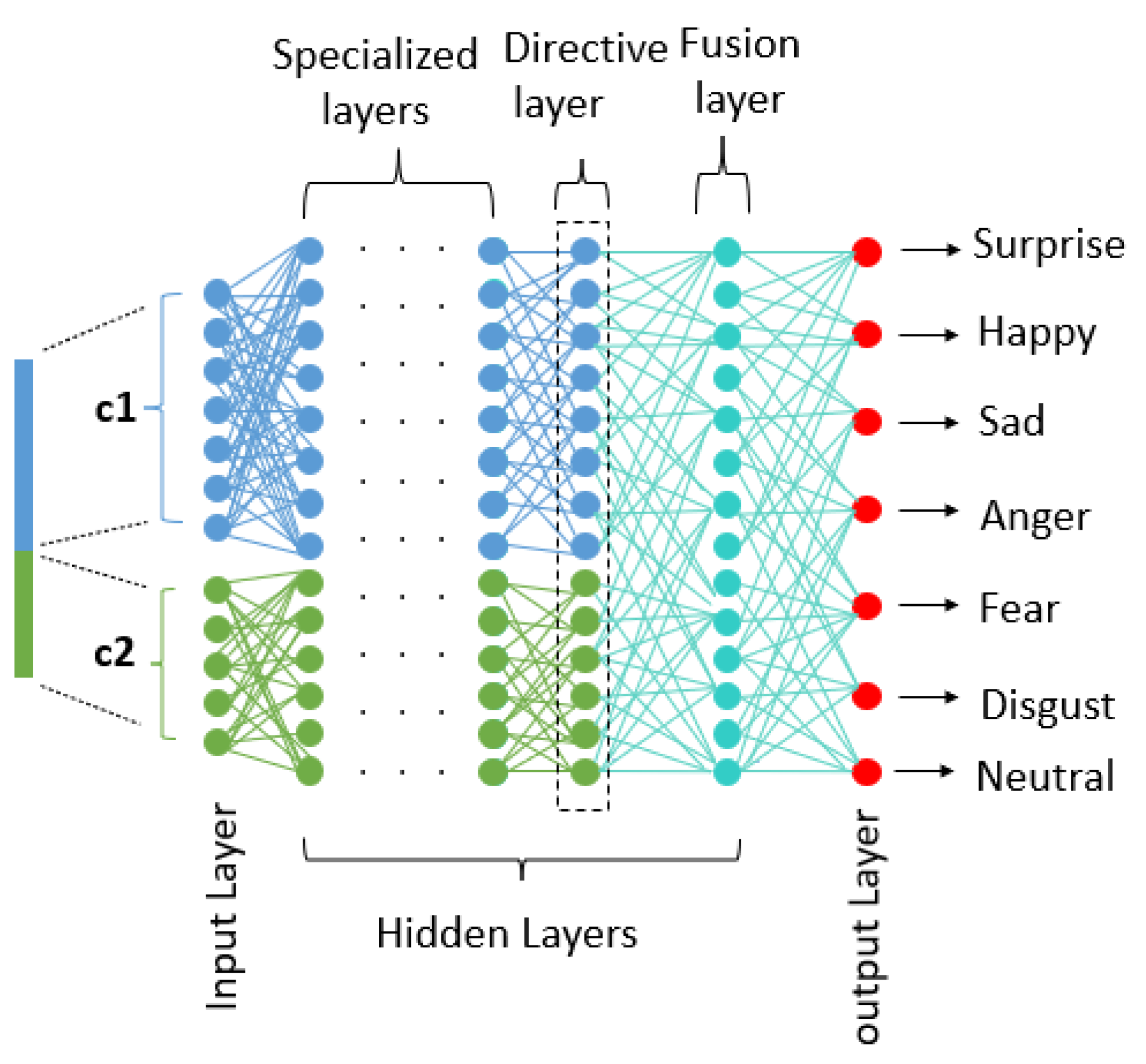
The Meaningful Neural Network (MNN), is a novel neural network model that was first invented by [41], which allows learning features from different architecture/algorithm/descriptive vectors representing data of different modalities, i.e., sound, image, text, etc., in a meaningful way.
The main idea of MNN is to dedicate a part named (specialized layers) of this network for learning each input vector component. Indeed, the learning of the latter’s characteristics is realized independently in a significant manner.
The MNN Architecture contains three types of layers show (Figure 3):
  • Specialized layers: Sets of neurons that are trained specifically to extract and learn the representations of the input vector components are present in each of these layers. Depending on how many components the input vector contains, we can often have any number of neuron sets. The weights’ calculation and updating during the gradient backpropagation step can be expressed as follows:
    Forward Propagation:
    z j c ( l ) = Ψ ( k = 1 T ( l 1 ) w ( k j ) ( l ) a k ( l 1 ) + b j ( l ) )
    c : the component numbers, T ( l 1 ) : the number of neurons belonging to the layer l 1 that concerns the component c , w ( k j ) ( l ) : the weight that connects the neuron j belonging to the layer l that concerns the component with the neuron belonging to the layer l 1 of the component c , a k ( l 1 ) : the output of the neuron k belonging to layer l 1 of the component c , b j ( l ) : the bias connected to the neuron j and belonging to layer l of component c .
    Backward Propagation:
    δ j c ( l ) = σ ( z j l ) k = 1 n ( l + 1 ) w ( j k ) ( l + 1 ) δ k ( l + 1 )
    E w ( i j ) c ( l ) = a i c ( l 1 ) δ j c ( l )
    E b j c ( l ) = δ j c ( l )
  • Directive layer: One directive layer is present in the suggested architecture. While the other side is fully connected, the left side is semi-connected. By taking into consideration the two sets of neurons for the specialized layers, this layer enables the control of error propagation.
    Forward Propagation:
    z j c ( l ) = Ψ ( k = 1 T ( l 1 ) w ( k j ) ( l ) a k ( l 1 ) + b j ( l ) )
    Backward Propagation:
    δ j c ( l ) = σ ( z j l ) k = 1 n ( l + 1 ) w ( j k ) ( l + 1 ) δ i ( l + 1 )
    E w ( i j ) c ( l ) = a i c ( l 1 ) δ j c ( l )
    E b j c ( l ) = δ j c ( l )
  • Fusing Layer: This layer is completely connected. It enables the merging of learned representations from earlier levels.
    Forward Propagation:
    z J c ( l ) = Ψ ( k = 1 T ( l 1 ) w ( k j ) ( l ) a k ( l 1 ) + b j ( l ) )
    c : the component numbers, T ( l 1 ) : the number of neurons belonging to the layer l 1 that concerns the component c, w ( k j ) ( l ) : the weight that connects the neuron j belonging to the layer l that concerns the component with the neuron belonging to the layer l 1 of the component c, a k ( l 1 ) : the output of the neuron k belonging to layer l 1 , b i ( l ) : the bias connected to the neuron j and belonging to layer l of component c.
    Backward Propagation:
    δ i c ( l ) = σ ( z j l ) k = 1 n ( l + 1 ) w ( j k ) ( l + 1 ) δ k ( l + 1 )
    E w ( i j ) c ( l ) = a i c ( l 1 ) δ j c ( l )  
    E b j c ( l ) = δ j c ( l )  

4. Proposed Method

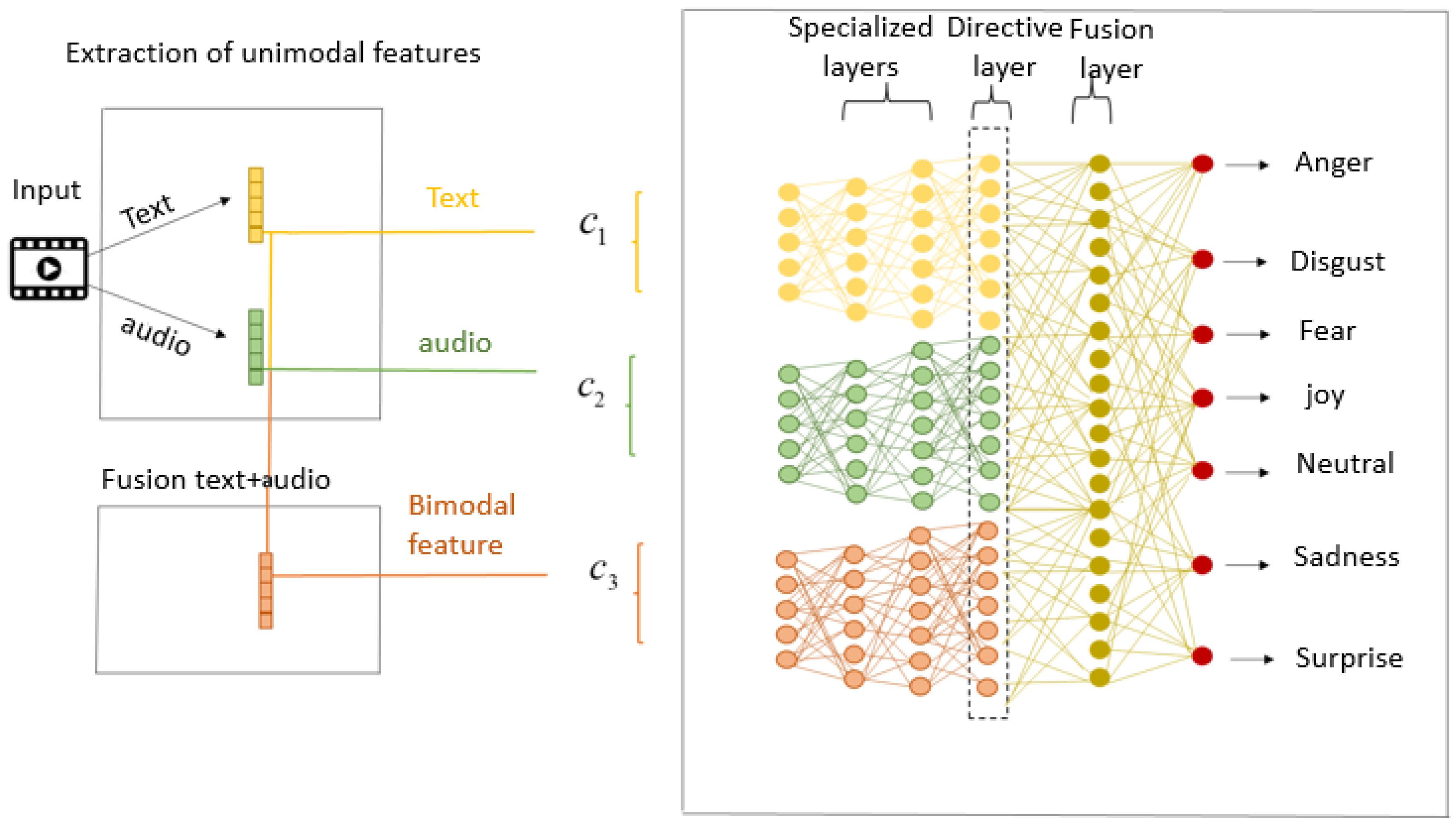
The proposed method consists of three steps presented in the Figure 4 below: the first one is devoted to extracting the features of each single modality (unimodal). The second step is designed to merge the two modalities audio and text (bimodal). While the third one is concerned with the classification of the three inputs (audio, text, and bimodal) concatenated in the same vector using MNN to predict emotions.

4.1. Extraction of Unimodal Features

Let D = { v 1 , v 2 , v 3 , , v n } , be the database that contains n videos, each video v i = { u i 1 , u i 2 , u i 3 , , u i m } is represented by a set of utterances noted u i j with m the number of utterances in the video v i . We will follow the same sequence of [42] to extract the features of each statement independently. For the text modality, their features will be passed to an LSTM network to allow consecutive utterances in a video to represent relevant information in the feature extraction process.

4.1.1. Extraction of Text Modality

The first step in extracting the text modality is to prepare and transform the text of the utterances into a digital format. First, we represent each utterance as the concatenation of vectors for constituent words. In our work, we used GloVe, which is a publicly available word representation tool based on global frequency statistics [43], with a dimensionality equal to 300 pre-trained on 42 billion vocabulary words. This dictionary provides a 300-dimensional vector for each word. Exploiting this tool, it was thought to use CNN to extract the features of each utterance given its high discrimination capability. In sequence classification, each utterance depends on the other utterances in the same sequence. The statements in a video maintain a sequence. In a video, we assume that there is a high probability of dependence between statements with respect to their sentimental cues. In particular, we argue that when classifying an utterance, the other utterances may provide important contextual information. Thus, a model is needed that takes into account these interdependencies and the effect they may have on the target utterance. To capture this flow of informational triggers between utterances, we use a recurrent neural network (RNN) based on LSTM [44] to extract contextual information based on the results obtained from CNN.
For the CNN, the input consists of the 300-dimensional pre-trained GloVe vectors. The proposed approach consists of three convolution layers: the first one contains 40 filters of size 3 × 3, and the second and the third layer contain, respectively, 100 and 150 filters of the same size (4 × 4). Each convolution layer uses a Stride equal to 2 and an identical Padding. At the end of each convolution layer, we apply the ReLu activation function. The pooling layer comes after each convolution layer. We chose the Max pooling with a 2 × 2 filter. The convoluted features are then concatenated and introduced into a fully connected layer of 1611 dimensions, whose activations form the representation of the statement.
The feature vector of the text generated by the CNN for each utterance will be grouped in a matrix that will be transmitted to the LSTM as input. The LSTM is capable of learning long-term dependencies. Its special structure with input, output, and forgetting gates controls the identification of the long-term sequence pattern. The process of the text vector is presented in the Figure 5.

4.1.2. Extraction of Audio Modality

To extract acoustic features. There are popular audio feature extraction toolkits available for free that are capable of extracting all fundamental features. We used The OpenSMILE Feature Extraction Toolkit [44], which brings together feature extraction algorithms from the speech processing and music information retrieval communities. The speech features captured by this collection include loudness, CHROMA, CENES, Mel cepstral coefficient features, and perceptual linear predictive cepstral features. Additionally, it records crucial elements such as format frequency and fundamental frequency. We computed three speech features—the MFCCS, loudness, and CHROMA features—using this package.
At a sliding window of 100 ms and a frame rate of 30 Hz, the audio features are extracted. Voice normalization is carried out and the voice intensity is thresholded to distinguish between voiced and unvoiced samples in order to compute the features. To combine with the other modalities, the generated features are further downsampled to 49.

4.2. The Fusion of Text and Audio Modalities

Fusion is one of the original topics in multimodal machine learning. In this context, we have developed a third modality to study the characteristics of text and audio fusion. We believe that this resulting vector can be used to effectively improve the classification effect.
A feature vector of 49 dimensions from the acoustic network and a feature vector of 1611 dimensions from the textual network are merged into a single vector that will present the modality (bimodal) that will be used later as a third component of the MNN network to classify emotions.

4.3. Classification

After having prepared the input vector of our system, we arrive at the fundamental part, which consists of the classification of the emotions. For this, the choice of classifier is very important because it can also significantly impact the accuracy of the recognition.
In the field of emotion recognition, various classifiers have been used. Among the most common approaches, we can mention the Gaussian mixture model (GMM) [45], the hidden Markov model (HMM) [46], the neural network (NN) [47], the SVM [48], AdaBoost [49], etc.
In our case, we used the MNN [41]. Its architecture is characterized by significant learning, which is very adapted to our system. As far as we know, most of the architectures that use the concatenation of feature vectors do not take into account the different components of the resulting vector. In fact, they consider this vector as a single entity while ignoring its constituent components. On the other hand, the MNN network architecture allows the components of the global feature vector to be learned in a meaningful way. It dedicates to each of its components a set of neurons belonging to a number of hidden layers.
The input vector of our system consists of three components: the text component with dimension 1611, the audio component with dimension 49, and the bimodal component with dimension 898.
At the input of the classification step, each input vector component is made of a number of neurons. We choose 500 neurons for text, 50 neurons for audio, and 300 for bimodal. The first 2 layers, named specialized layers, are accessed by the 3 components. Then, they move to the Directive layer and, lastly, to the fusion layer, before recognizing the final emotions. The passage from one layer to another is performed with a minimal number of neurons compared to the previous layer and by calculating the weights and their updates at each passage, with the backward and forward propagation formulas mentioned in Section 3. Moreover, the audio component keeps the same result at the fusion level even by increasing the number of neurons at the input. Comparing the components, the number of neurons used in text and bimodal at the input of the classification step is higher than the audio component. This justifies the absence of neurons for the audio component in the directive layer.
The parameters of each component within the MNN network are represented in the Table 1 below.

5. Proposed Experimental Results and Discussion

5.1. Computational Environment

The Python toolbox was used to implement our proposed model. The experiments were executed on an Asus desktop (Taiwanese multinational computer and phone hardware and electronics company headquartered in Beitou District, Taipei, Taiwan), which has 8 GB RAM, Intel (R) Core (TM) i7-8550U CPU @ 1.80 GHz (8 CPUs), ~2.0 GHz, and Windows 10 as the operating system. Moreover, the Google Colab cloud service was used to train the proposed architecture.

5.2. Dataset

The Multimodal Emotion Lines Dataset (MELD) [13,14] is an evolved version of the EmotionLines Dataset. MELD has the same dialogue instances as those available in EmotionLines, but additionally includes audio, visual modality, and text. The MELD has over 1400 dialogues and 13,000 utterances from the Friends television series, with the dialogue samples grouped into 1039 for training, 114 for validation, and 280 for testing, and the utterances samples grouped into 9989 for training, 1109 for validation, and 2610 for testing.
The utterances in each dialogue were annotated with any of these seven emotions (Anger, Disgust, Fear, Joy, Neutral, Sadness, and Surprise) were coded as 0, 1, 2, 3, 4, 5, and 6 annotation labels. This annotation list was extended with two additional emotion labels: Neutral and Non-Neutral. Label distributions in the training, validation, and test datasets can be seen in Table 2. Figure 6 shows an example of dialogue extracted from the MELD dataset.

5.3. Evaluation Metrics

We evaluated the performance of our model using the following evaluation metrics: Accuracy, Precision, Recall, and F1-score. The expression of these metrics is given as follows:
  • Accuracy: the easiest performance metric to understand is accuracy, which is just the proportion of correctly predicted observations to all observations. T P + T N T P + F N + T N + F P
  • Recall: is a metric for how well a model detects True Positives. T P T P + F N
  • Precision: is the ratio of accurately anticipated positive observations to all actual class observations—yes. T P T P + F P
  • F1-score: is the average of Precision and Recall, weighted. 2 Pr e c i s i o n * Re c a l l Pr e c i s i o n + Re c a l l
where TP, TN, FN, and FP are defined respectively as:
(TP) A test outcome that accurately detects the existence of a condition or characteristic.
(TN) A test outcome that accurately demonstrates the absence of a condition or characteristic.
(FN) A test result that falsely suggests the presence of a certain condition or attribute.
(FP) A test result that falsely suggests the absence of a certain condition or attribute.
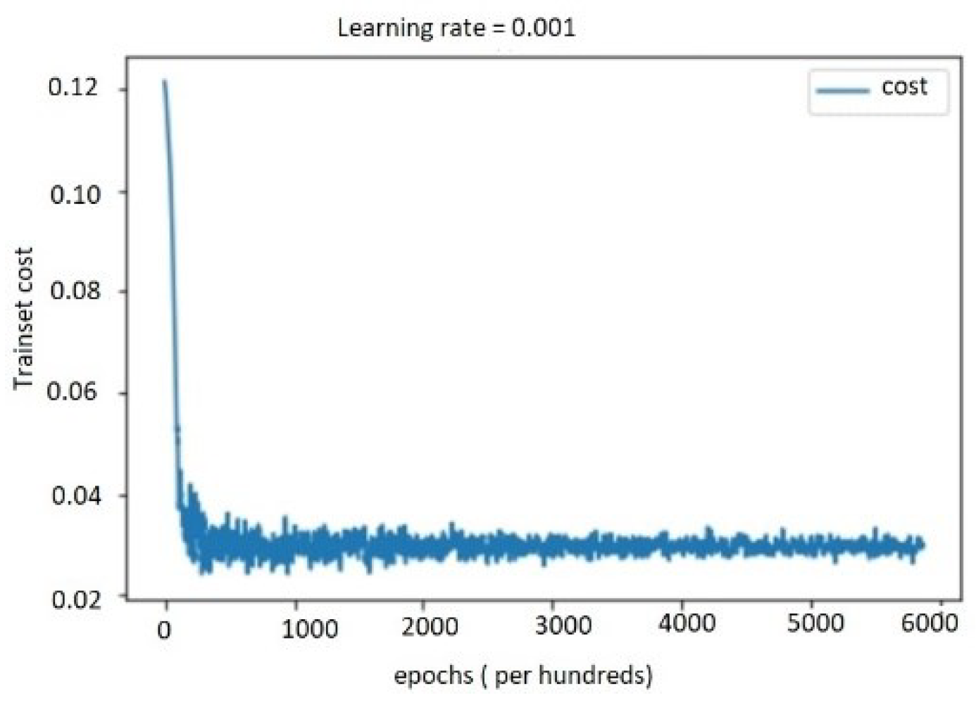
Moreover, we elaborated the macro average and weighted average metrics, we mounted the cost, training accuracy, and training accuracy/validation accuracy curves according to the epochs, and finally we displayed the confusion matrix.

5.4. Performance Evaluation

We evaluated the performance of our system through the following steps: the first contains a detailed study of the audio, text, and bimodal (text + audio) modalities; the second presented a test on the multimodal system, and the third, a comparison with existing works.

5.4.1. Performance Study on Audio, Text, and Bimodal Modalities

The training, validation, and test sets for the MELD dataset were already separated, as was previously announced. Since we needed the findings, we constructed our model, adjusted the training hyperparameters based on the training and validation sets, and tested the model on the test set.
The tables above display the metrics of the three modalities obtained with the MELD dataset. Each metric for a given modality generates different values for every emotion. This block of values (modality, emotion) is called the test classification results.
From Table 3, the maximum value of the precision for the text modality concerns the anger emotion (90%), and with a value of 98% for the disgust emotion in the two other modalities. Concerning the metric Recall, the text modality reaches a maximum value of 95% for the emotion surprise, 97% for the audio modality with the disgust emotion, and 98% for the same emotion for the bimodal modality. Regarding the third metric, F1-score registers 89% as a value for the modality text (emotion surprise), a value of 97% for audio, and 98% for bimodal with emotion disgust.
Concerning the values of Macro average and weighted average metrics, they gave a general view on all the samples of the dataset used.
According to Table 4, the bimodal has the highest value of Accuracy with a rate of 86.51%. In second place, the text modality achieves 83.98% as a value, and in last place, the audio modality has a value of 81.79%.
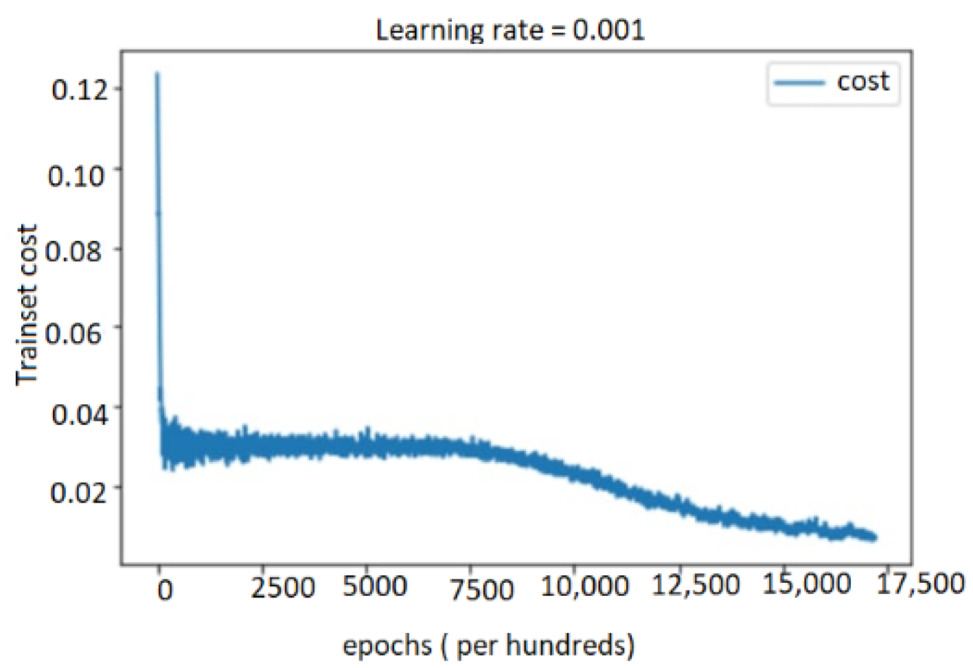
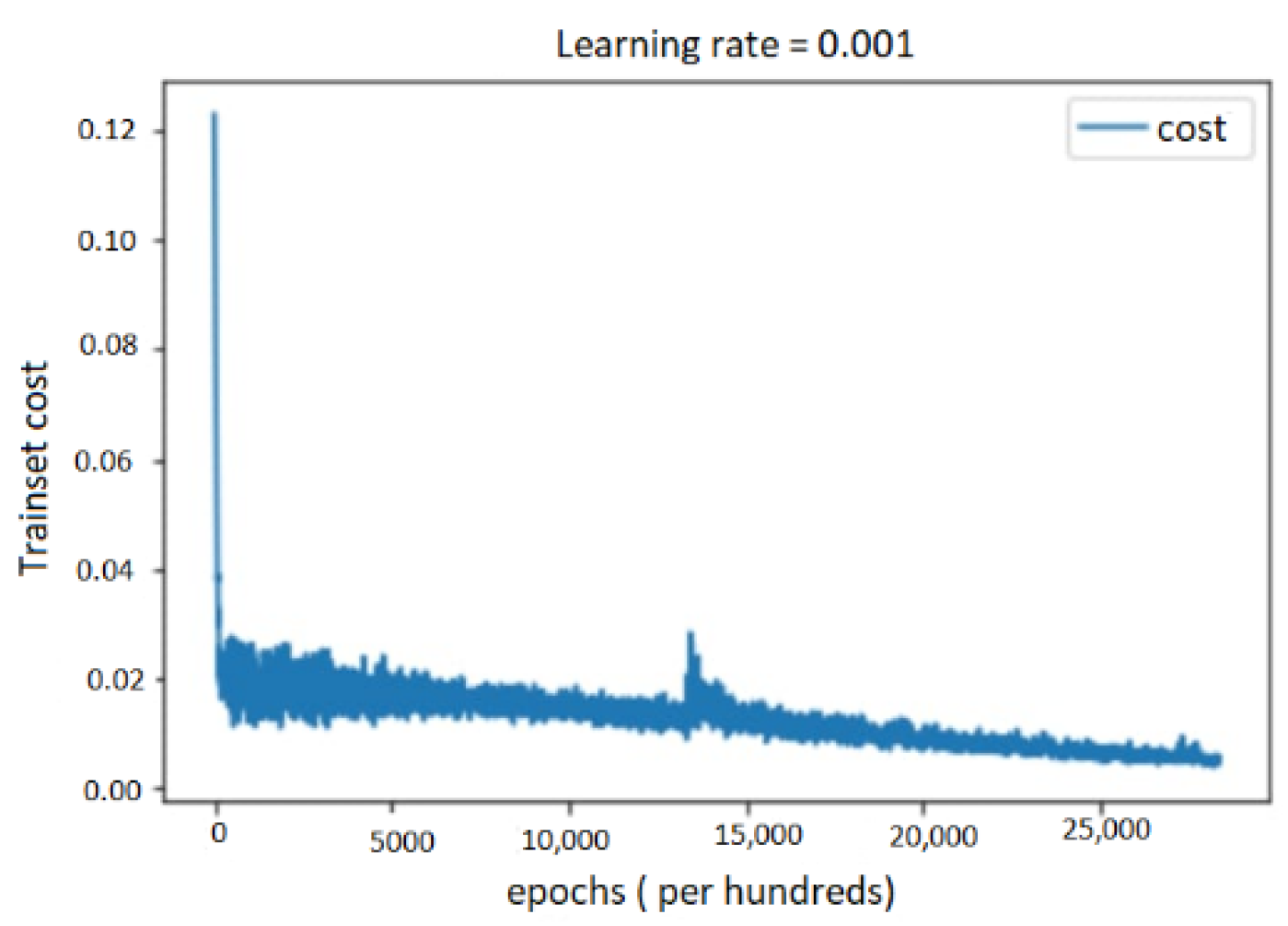
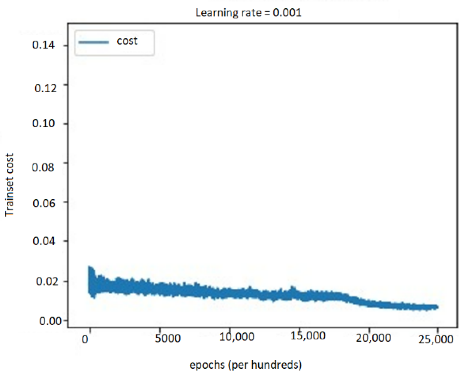
Figure 7, Figure 8 and Figure 9 show the training cost of the three modalities. We can see that the maximum value is reached around 0 epochs and is reduced by increasing the number of epochs. The cost achieves the value of 0.0115 for the text modality, 0.0634 for the audio, and 0.0046 for the bimodal.
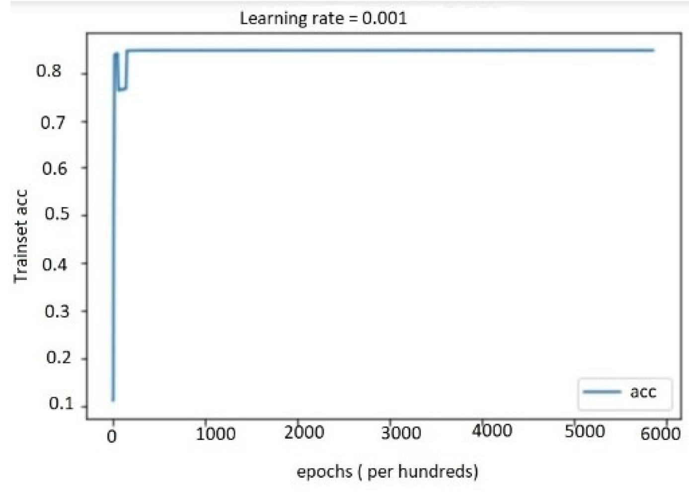
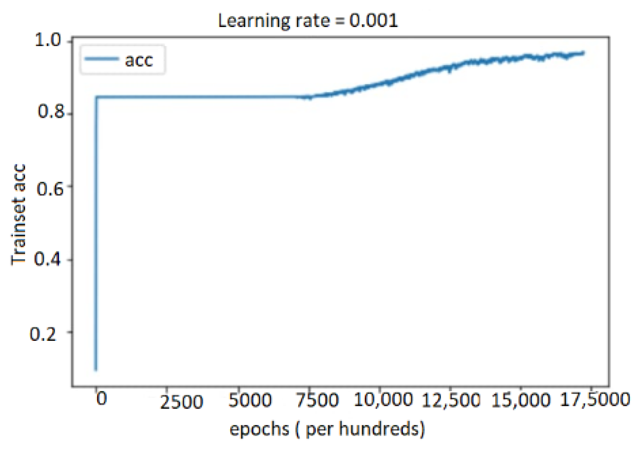
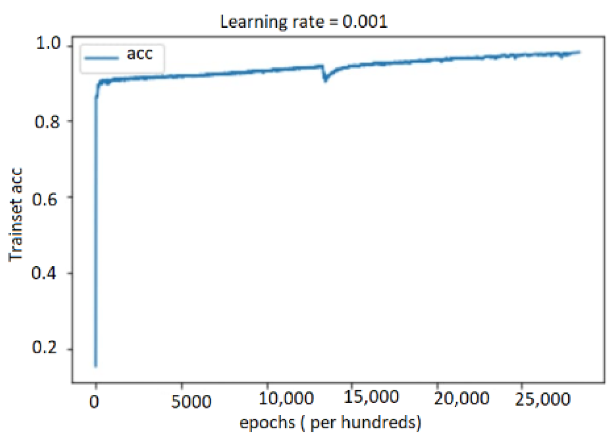
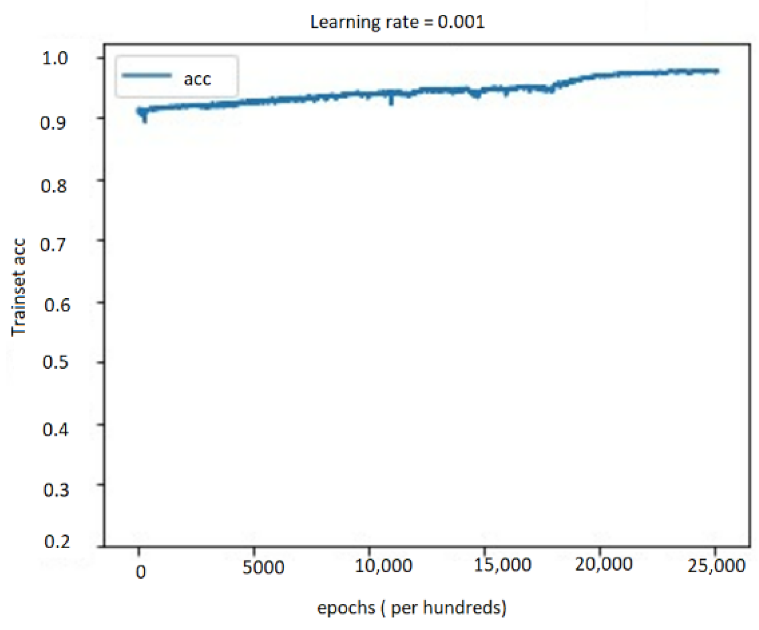
In Figure 10, Figure 11 and Figure 12, we visualize the training accuracy of the three modalities. We notice that for the latter, a maximum value is reached, then a decrease to resume a maximum value, which stabilizes from a certain number of epochs. For the text modality, the maximum value of training accuracy is 83.76%. For the audio modality, it is 96.92%. Then, it reaches 98.03% as the value for the bimodal.
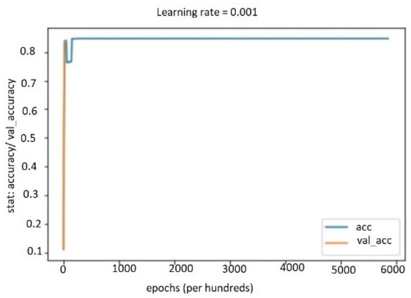
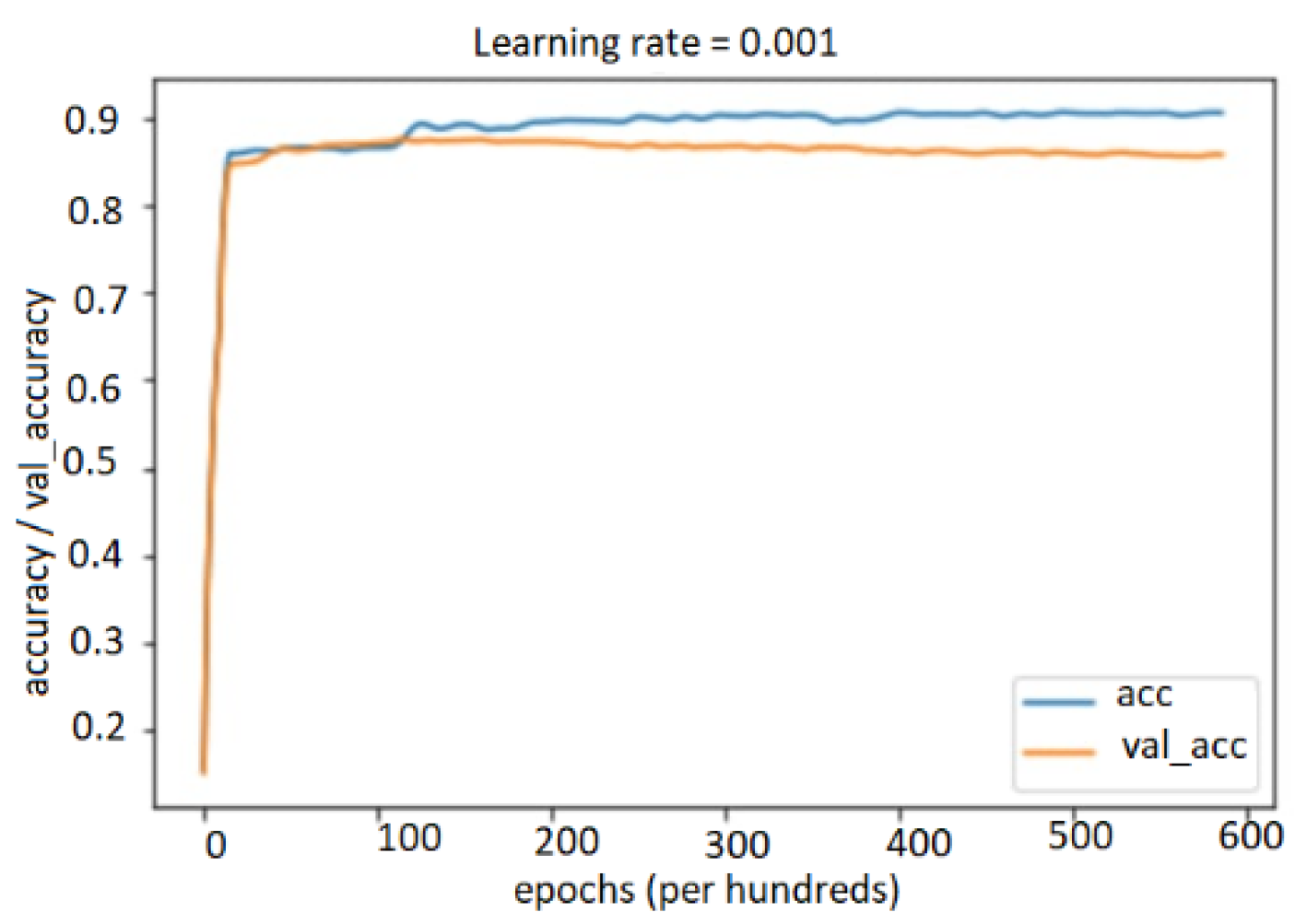
These three figures (Figure 13, Figure 14 and Figure 15) show the variation in training accuracy and validation accuracy according to the number of epochs. We notice that the three curves are almost superimposed and reach close maximum values.

5.4.2. Performance Results on Multimodal System

Above, we have studied the recognition of emotions for the text, audio, and bimodal modalities separately. In what follows, we go on with the multimodal modality of the proposed method.
Using the multimodal system on the MELD dataset, we notice that the evaluation metrics reach a maximum value of 98% for the disgust emotion (Table 5). Comparing the single modalities, we can see equality between the bimodal and multimodal values, which is not the case. Our method performs better by recording an advanced decimal value (the values are rounded by the system).
The accuracy reaches 86.69%, where an improvement is detected with the use of a multimodal system.
Regarding the loss indicator (Figure 16), it registers the value of 0.0039, which is lower from a certain number of epochs compared to other previous systems. For training accuracy (Figure 17), the system reaches its peak with a value of 98.42%.
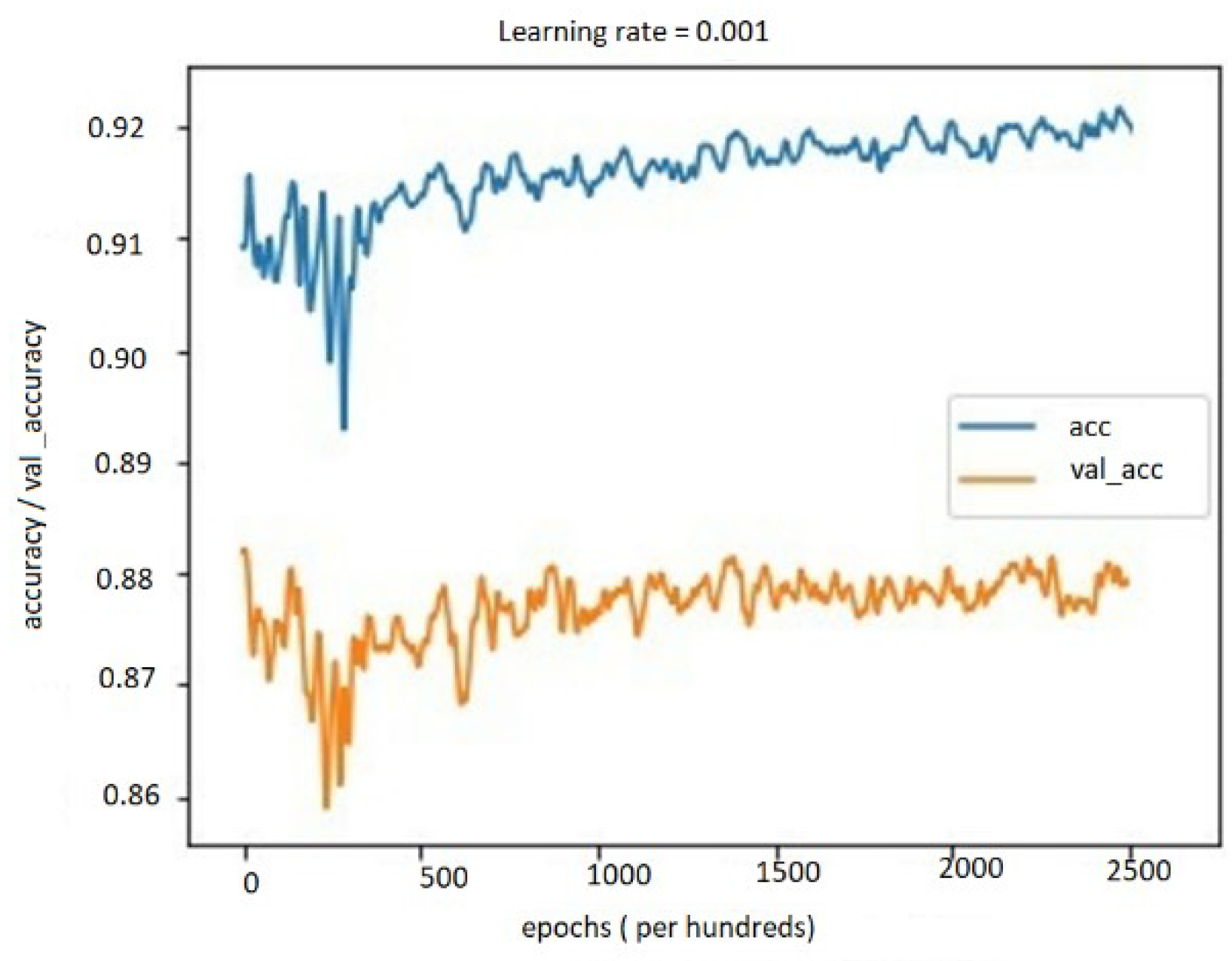
In Figure 18, the training accuracy and validation accuracy curves are almost superimposed and this regenerates the absence of the overfitting problem.
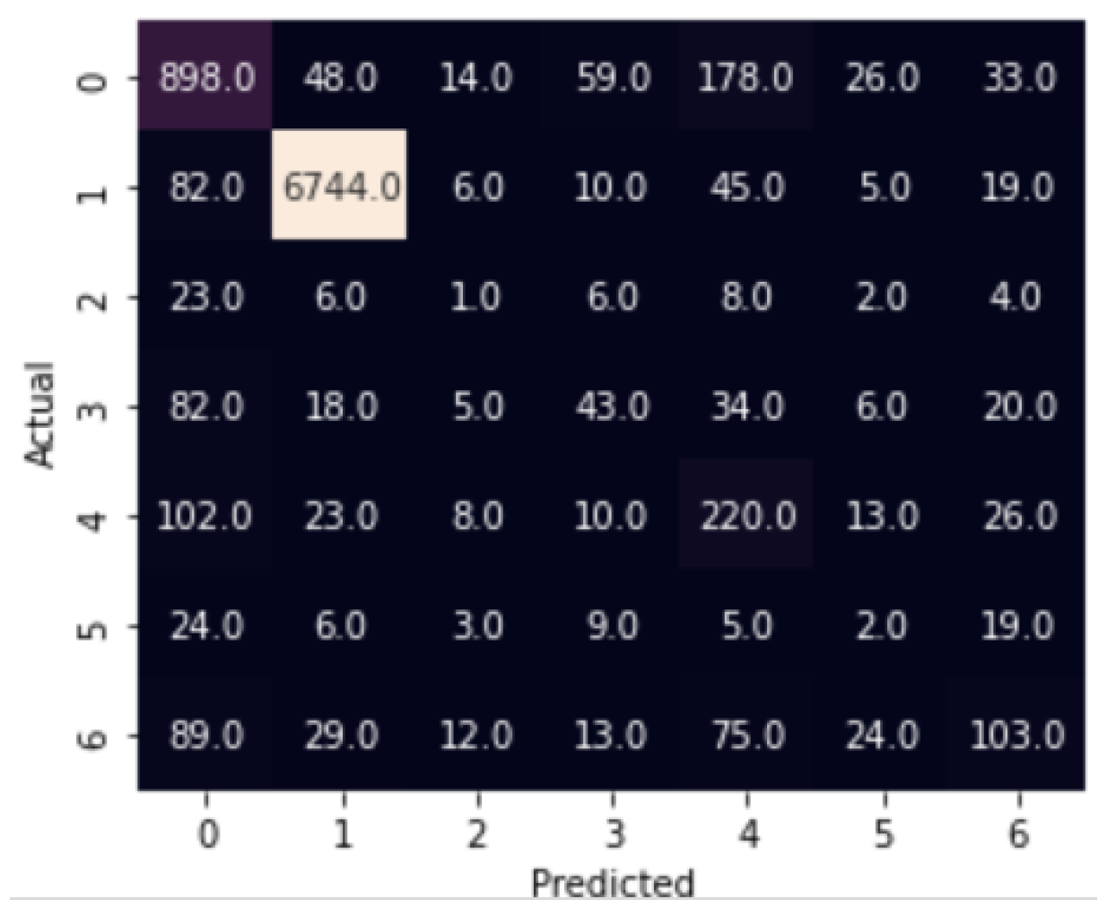
In the multimodal confusion matrix (Figure 19), the maximum value of the true label is 6744 for the disgust class. This represents the high value in this matrix.
Our multimodal fusion model outperformed the unimodal findings, according to all evaluation metrics.

5.5. Comparison with State-of-the-Art Methods

In order to evaluate the performance of our approach, we have compared it with other state-of-the-art methods. We have considered relevant approaches that give a good Accuracy regarding the MELD dataset, and we have drawn a comparison with the methods proposed by [34,35,36,37]. The obtained results are presented in Table 6.
Table 6 shows that our proposed method achieves higher Accuracy that matches the state-of-the-art performance and propounds its robustness in multimodal emotion classification.

6. Conclusions and Futures Work

Through this work, we have proposed a multimodal emotion recognition system for conversations. This system consists of a model with two different modalities (text, audio) that are respectively extracted with (CNN, LSTM) and OpenSmile. A third modality is built from the fusion of the audio and text features into a single vector. All three modalities feed a meaningful neural network and result in allowing good feature learning to accurately identify emotional states. Moreover, due to the meaningful neural network structure, the proposed architecture can be robustly extended to a larger set of input modalities. The obtained results demonstrate the performance of our proposed approach. Regarding our future works, we plan to deeply study temporal performance in order to construct a real-time multimodal emotion recognition system focusing on the visual modality as well as evaluating other multimodal datasets.

Author Contributions

Conceptualization, C.B.; Supervision, J.R., M.A.M., and H.T.; Writing—original draft, H.F.; Writing—review and editing, H.F. All authors have read and agreed to the published version of the manuscript.

Funding

This research received no external funding.

Institutional Review Board Statement

Ethical review and approval were waived for this study due to the detection of emotions using human faces. The last shown in the paper are cited from the public dataset MELD.

Informed Consent Statement

The human faces shown in the paper are cited from the public dataset MELD, so no consent is needed.

Data Availability Statement

We used the MELD dataset available in: https://affective-meld.github.io/ (accessed on 15 July 2022).

Conflicts of Interest

The authors declare no conflict of interest.

References

  1. Definition of ‘Emotion’. In Merriam-Webster Dictionary; Merriam-Webster: Springfield, MA, USA, 2012.
  2. Perveen, N.; Roy, D.; Chalavadi, K.M. Facial Expression Recognition in Videos Using Dynamic Kernels. IEEE Trans. Image Process. 2020, 29, 8316–8325. [Google Scholar] [CrossRef] [PubMed]
  3. Chen, L.; Ouyang, Y.; Zeng, Y.; Li, Y. Dynamic Facial Expression Recognition Model Based on BiLSTM-Attention. In Proceedings of the 2020 15th International Conference on Computer Science & Education (ICCSE), IEEE, Delft, The Netherlands, 18–22 August 2020; pp. 828–832. [Google Scholar]
  4. Zeebaree, S.; Ameen, S.; Sadeeq, M. Social Media Networks Security Threats, Risks and Recommendation: A Case Study in the Kurdistan Region. Int. J. Innov. Creat. Change 2020, 13, 349–365. [Google Scholar]
  5. Al-Sultan, M.R.; Ameen, S.Y.; Abduallah, W.M. Real Time Implementation of Stegofirewall System. Int. J. Comput. Digit. Syst. 2019, 8, 498–504. [Google Scholar]
  6. Baimbetov, Y.; Khalil, I.; Steinbauer, M.; Anderst-Kotsis, G. Using Big Data for Emotionally Intelligent Mobile Services through Multi-Modal Emotion Recognition. In Proceedings of the International Conference on Smart Homes and Health Telematics, Denver, CO, USA, 25–27 June 2014; Springer: Berlin/Heidelberg, Germany, 2015; pp. 127–138. [Google Scholar]
  7. Bianchi-Berthouze, N.; Lisetti, C.L. Modeling Multimodal Expression of User’s Affective Subjective Experience. User Model. User-Adapt. Interact. 2002, 12, 49–84. [Google Scholar] [CrossRef]
  8. Abdullah, S.M.S.A.; Ameen, S.Y.A.; Sadeeq, M.A.M.; Zeebaree, S. Multimodal Emotion Recognition Using Deep Learning. J. Appl. Sci. Technol. Trends 2021, 2, 52–58. [Google Scholar] [CrossRef]
  9. Said, Y.; Barr, M. Human Emotion Recognition Based on Facial Expressions via Deep Learning on High-Resolution Images. Multimed. Tools Appl. 2021, 80, 25241–25253. [Google Scholar] [CrossRef]
  10. Anagnostopoulos, C.-N.; Iliou, T.; Giannoukos, I. Features and Classifiers for Emotion Recognition from Speech: A Survey from 2000 to 2011. Artif. Intell. Rev. 2015, 43, 155–177. [Google Scholar] [CrossRef]
  11. Thakur, N.; Han, C.Y. An Exploratory Study of Tweets about the SARS-CoV-2 Omicron Variant: Insights from Sentiment Analysis, Language Interpretation, Source Tracking, Type Classification, and Embedded URL Detection. COVID 2022, 2, 1026–1049. [Google Scholar] [CrossRef]
  12. Alarcao, S.M.; Fonseca, M.J. Emotions Recognition Using EEG Signals: A Survey. IEEE Trans. Affect. Comput. 2017, 10, 374–393. [Google Scholar] [CrossRef]
  13. Poria, S.; Hazarika, D.; Majumder, N.; Naik, G.; Cambria, E.; Mihalcea, R. MELD: A Multimodal Multi-Party Dataset for Emotion Recognition in Conversations. In Proceedings of the 57th Annual Meeting of the Association for Computational Linguistics, Florence, Italy, 28 July–2 August 2019; Association for Computational Linguistics: Florence, Italy, 2019; pp. 527–536. [Google Scholar]
  14. Chen, S.-Y.; Hsu, C.-C.; Kuo, C.-C.; Ku, L.-W. EmotionLines: An Emotion Corpus of Multi-Party Conversations. arXiv 2018, arXiv:1802.08379. [Google Scholar]
  15. Busso, C.; Bulut, M.; Lee, C.-C.; Kazemzadeh, A.; Mower, E.; Kim, S.; Chang, J.N.; Lee, S.; Narayanan, S.S. IEMOCAP: Interactive Emotional Dyadic Motion Capture Database. Lang. Resour. Eval. 2008, 42, 335–359. [Google Scholar] [CrossRef]
  16. Zadeh, A.; Zellers, R.; Pincus, E.; Morency, L.-P. MOSI: Multimodal Corpus of Sentiment Intensity and Subjectivity Analysis in Online Opinion Videos. arXiv 2016, arXiv:1606.06259. [Google Scholar]
  17. Choi, W.Y.; Song, K.Y.; Lee, C.W. Convolutional Attention Networks for Multimodal Emotion Recognition from Speech and Text Data. In Proceedings of the Grand Challenge and Workshop on Human Multimodal Language (Challenge-HML), Melbourne, Australia, 20 July 2018; pp. 28–34. [Google Scholar]
  18. Tzirakis, P.; Trigeorgis, G.; Nicolaou, M.A.; Schuller, B.W.; Zafeiriou, S. End-to-End Multimodal Emotion Recognition Using Deep Neural Networks. IEEE J. Sel. Top. Signal Process. 2017, 11, 1301–1309. [Google Scholar] [CrossRef]
  19. Poria, S.; Chaturvedi, I.; Cambria, E.; Hussain, A. Convolutional MKL Based Multimodal Emotion Recognition and Sentiment Analysis. In Proceedings of the 2016 IEEE 16th International Conference on Data Mining (ICDM), IEEE, Barcelona, Spain, 12–15 December 2016; pp. 439–448. [Google Scholar]
  20. Maat, L.; Pantic, M. Gaze-X: Adaptive, Affective, Multimodal Interface for Single-User Office Scenarios. In Artifical Intelligence for Human Computing, Proceedings of the 8th International Conference on Multimodal Interfaces, Banff, AB, Canada, 2–4 November 2006; Springer: Berlin/Heidelberg, Germany, 2007; pp. 251–271. [Google Scholar]
  21. Su, Q.; Chen, F.; Li, H.; Yan, N.; Wang, L. Multimodal Emotion Perception in Children with Autism Spectrum Disorder by Eye Tracking Study. In Proceedings of the 2018 IEEE-EMBS Conference on Biomedical Engineering and Sciences (IECBES), IEEE, Sarawak, Malaysia, 3–6 December 2018; pp. 382–387. [Google Scholar]
  22. Nemati, S.; Rohani, R.; Basiri, M.E.; Abdar, M.; Yen, N.Y.; Makarenkov, V. A Hybrid Latent Space Data Fusion Method for Multimodal Emotion Recognition. IEEE Access 2019, 7, 172948–172964. [Google Scholar] [CrossRef]
  23. Prasad, G.; Dikshit, A.; Lalitha, S. Sentiment and Emotion Analysis for Effective Human-Machine Interaction during Covid-19 Pandemic. In Proceedings of the 2021 8th International Conference on Signal Processing and Integrated Networks (SPIN), IEEE, Noida, India, 26–27 August 2021; pp. 909–915. [Google Scholar]
  24. Priyasad, D.; Fernando, T.; Denman, S.; Sridharan, S.; Fookes, C. Attention Driven Fusion for Multi-Modal Emotion Recognition. In Proceedings of the ICASSP 2020-2020 IEEE International Conference on Acoustics, Speech and Signal Processing (ICASSP), IEEE, Barcelona, Spain, 4–8 May 2020; pp. 3227–3231. [Google Scholar]
  25. Sun, B.; Li, L.; Zhou, G.; Wu, X.; He, J.; Yu, L.; Li, D.; Wei, Q. Combining Multimodal Features within a Fusion Network for Emotion Recognition in the Wild. In Proceedings of the 2015 ACM on International Conference on Multimodal Interaction, Seattle, WA, USA, 9–13 November 2015; pp. 497–502. [Google Scholar]
  26. Schuller, B.; Valster, M.; Eyben, F.; Cowie, R.; Pantic, M. Avec 2012: The Continuous Audio/Visual Emotion Challenge. In Proceedings of the 14th ACM International Conference on Multimodal Interaction, Santa Monica, CA, USA, 22–26 October 2012; pp. 449–456. [Google Scholar]
  27. Cevher, D.; Zepf, S.; Klinger, R. Towards Multimodal Emotion Recognition in German Speech Events in Cars Using Transfer Learning. arXiv 2019, arXiv:1909.02764. [Google Scholar]
  28. Georgiou, E.; Papaioannou, C.; Potamianos, A. Deep Hierarchical Fusion with Application in Sentiment Analysis. In Proceedings of the Interspeech, Graz, Austria, 15–19 September 2019; pp. 1646–1650. [Google Scholar]
  29. Bahreini, K.; Nadolski, R.; Westera, W. Data Fusion for Real-Time Multimodal Emotion Recognition through Webcams and Microphones in e-Learning. Int. J. Hum. Comput. Interact. 2016, 32, 415–430. [Google Scholar] [CrossRef]
  30. Slavova, V. Towards Emotion Recognition in Texts–a Sound-Symbolic Experiment. Int. J. Cogn. Res. Sci. Eng. Educ. (IJCRSEE) 2019, 7, 41–51. [Google Scholar] [CrossRef]
  31. Pan, Z.; Luo, Z.; Yang, J.; Li, H. Multi-Modal Attention for Speech Emotion Recognition. arXiv 2020, arXiv:2009.04107. [Google Scholar]
  32. Krishna, D.N.; Patil, A. Multimodal Emotion Recognition Using Cross-Modal Attention and 1D Convolutional Neural Networks. In Proceedings of the Interspeech, Shanghai, China, 25–29 October 2020; pp. 4243–4247. [Google Scholar]
  33. Huang, J.; Li, Y.; Tao, J.; Lian, Z.; Wen, Z.; Yang, M.; Yi, J. Continuous Multimodal Emotion Prediction Based on Long Short Term Memory Recurrent Neural Network. In Proceedings of the 7th Annual Workshop on Audio/Visual Emotion Challenge, Mountain View, CA, USA, 23–27 October 2017; pp. 11–18. [Google Scholar]
  34. Lian, Z.; Liu, B.; Tao, J. CTNet: Conversational Transformer Network for Emotion Recognition. IEEE/ACM Trans. Audio Speech Lang. Process. 2021, 29, 985–1000. [Google Scholar] [CrossRef]
  35. Ma, H.; Wang, J.; Lin, H.; Pan, X.; Zhang, Y.; Yang, Z. A Multi-View Network for Real-Time Emotion Recognition in Conversations. Knowl. Based Syst. 2022, 236, 107751. [Google Scholar] [CrossRef]
  36. Siriwardhana, S.; Kaluarachchi, T.; Billinghurst, M.; Nanayakkara, S. Multimodal Emotion Recognition with Transformer-Based Self Supervised Feature Fusion. IEEE Access 2020, 8, 176274–176285. [Google Scholar] [CrossRef]
  37. Xie, B.; Sidulova, M.; Park, C.H. Robust Multimodal Emotion Recognition from Conversation with Transformer-Based Crossmodality Fusion. Sensors 2021, 21, 4913. [Google Scholar] [CrossRef]
  38. LeCun, Y.; Bottou, L.; Bengio, Y.; Haffner, P. Gradient-Based Learning Applied to Document Recognition. Proc. IEEE 1998, 86, 2278–2324. [Google Scholar] [CrossRef]
  39. Hochreiter, S.; Schmidhuber, J. Long Short-Term Memory. Neural Comput. 1997, 9, 1735–1780. [Google Scholar] [CrossRef]
  40. Gers, F.A.; Schmidhuber, J.; Cummins, F. Learning to Forget: Continual Prediction with LSTM. Neural Comput. 2000, 12, 2451–2471. [Google Scholar] [CrossRef]
  41. Filali, H.; Riffi, J.; Aboussaleh, I.; Mahraz, A.M.; Tairi, H. Meaningful Learning for Deep Facial Emotional Features. Neural Process. Lett. 2022, 54, 387–404. [Google Scholar] [CrossRef]
  42. Poria, S.; Cambria, E.; Hazarika, D.; Majumder, N.; Zadeh, A.; Morency, L.-P. Context-Dependent Sentiment Analysis in User-Generated Videos. In Proceedings of the 55th Annual Meeting of the Association for Computational Linguistics (Volume 1: Long Papers), Vancouver, BC, Canada, 30 July–4 August 2017; pp. 873–883. [Google Scholar]
  43. Pennington, J.; Socher, R.; Manning, C.D. GloVe: Global Vectors for Word Representation. In Proceedings of the 2014 Conference on Empirical Methods in Natural Language Processing (EMNLP), Doha, Qatar, 25–29 October 2014; pp. 1532–1543. [Google Scholar]
  44. Eyben, F.; Wöllmer, M.; Schuller, B. Opensmile: The Munich Versatile and Fast Open-Source Audio Feature Extractor. In Proceedings of the 18th ACM International Conference on Multimedia, Firenze, Italy, 25–29 October 2010; pp. 1459–1462. [Google Scholar]
  45. Reynolds, D.A. Gaussian Mixture Models. Encycl. Biom. 2009, 741, 659–663. [Google Scholar]
  46. Eddy, S.R. Hidden Markov Models. Curr. Opin. Struct. Biol. 1996, 6, 361–365. [Google Scholar] [CrossRef]
  47. Wang, S.-C. Artificial Neural Network. In Interdisciplinary Computing in Java Programming; Springer: Berlin/Heidelberg, Germany, 2003; pp. 81–100. [Google Scholar]
  48. Noble, W.S. What Is a Support Vector Machine? Nat. Biotechnol. 2006, 24, 1565–1567. [Google Scholar] [CrossRef]
  49. Schapire, R.E. Explaining Adaboost. In Empirical Inference; Springer: Berlin/Heidelberg, Germany, 2013; pp. 37–52. [Google Scholar]
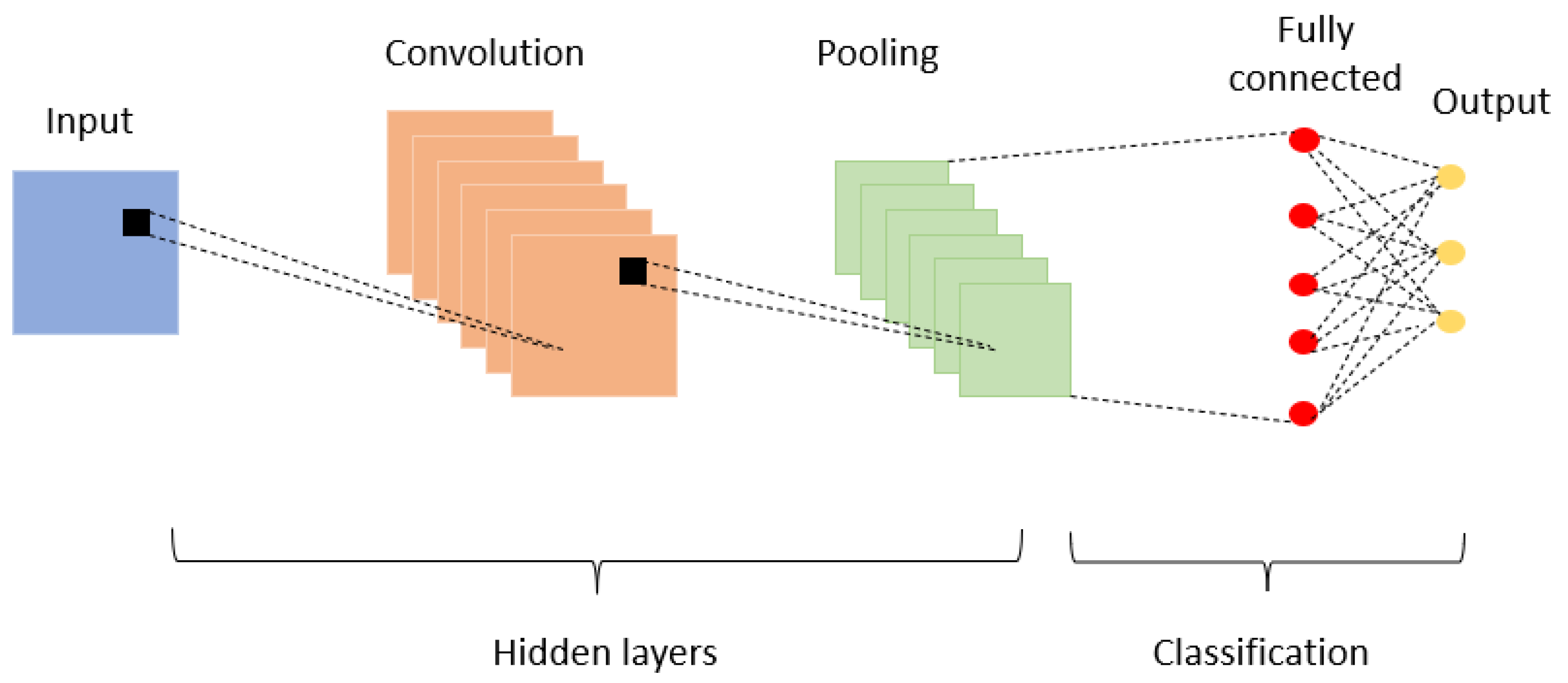
Figure 1. Architecture of a convolutional neural network.
Bdcc 06 00095 g001
Figure 2. Representation of LSTM cell.
Bdcc 06 00095 g002
Figure 3. General architecture of meaningful neural network.
Bdcc 06 00095 g003
Figure 4. General structure of our proposed approach.
Bdcc 06 00095 g004
Figure 5. The text vector extraction process.
Bdcc 06 00095 g005
Figure 6. An example of dialogue extract from MELD dataset [13,14].
Bdcc 06 00095 g006
Figure 7. Training cost versus epochs for text modality.
Bdcc 06 00095 g007
Figure 8. Training cost versus epochs for audio modality.
Bdcc 06 00095 g008
Figure 9. Training cost versus epochs for bimodal (text + audio) modality.
Bdcc 06 00095 g009
Figure 10. Training accuracy versus epochs for text modality.
Bdcc 06 00095 g010
Figure 11. Training accuracy versus epochs for audio modality.
Bdcc 06 00095 g011
Figure 12. Training accuracy versus epochs for bimodal (text + audio) modality.
Bdcc 06 00095 g012
Figure 13. Training accuracy/validation accuracy versus epochs for text modality.
Bdcc 06 00095 g013
Figure 14. Training accuracy/validation accuracy versus epochs for audio modality.
Bdcc 06 00095 g014
Figure 15. Training accuracy/validation accuracy versus bimodal (text + audio) modality.
Bdcc 06 00095 g015
Figure 16. Training cost versus epochs for the multimodal system.
Bdcc 06 00095 g016
Figure 17. Training accuracy versus epochs for the multimodal system.
Bdcc 06 00095 g017
Figure 18. Training accuracy/validation accuracy versus epochs for the multimodal system.
Bdcc 06 00095 g018
Figure 19. Multimodal confusion matrix of 7-class facial expression recognition results obtained by the MELD database.
Bdcc 06 00095 g019
Table 1. Classification parameters.
LayerComponents
C1 TextC2 AudioC3 Bimodal
DimensionNumber of
Neurones
Activation FunctionDimensionNumber of
Neurones
Activation FunctionDimensionNumber of
Neurones
Activation Function
Input1611500ReLu4950ReLu898300ReLu
Specialized layer 1 200ReLu 20ReLu 200ReLu
Specialized layer 2 50ReLu 7Softmax 50ReLu
Directive Layer 7Softmax -- 7Softmax
Fusion layer217Softmax217Softmax217Softmax
Output 7Softmax 7Softmax 7Softmax
Table 2. Distributions in the training, validation, and test datasets for each label.
AngerDisgustFearJoyNeutralSadnessSurprise
Train1109271268174347106831205
Dev1532240163470111150
Test34568504021256208281
Table 3. Classification report results for the MELD on text, audio, and bimodal modalities in the function of (Precision, Recall, and F1-score) (Unit = %).
EmotionModality
Text OnlyAudio OnlyBimodal (Text + Audio)
PrecisionRecallF1-ScorePrecisionRecallF1-ScorePrecisionRecallF1-Score
Anger908788555856727272
Disgust688074989797989898
Fear6035440004106
Joy76364891812231820
Neutral888888171918444645
Sadness824054312697
Surprise849589271419392933
Macro avg786669303029414040
Weighted avg848483828282878787
Table 4. The accuracy results of the single and bimodal modality.
ModalityAccuracy (%)
Audio only81.79
Text only83.98
Bimodal (text + audio)86.51
Table 5. Classification report results for the MELD on the multimodal system in the function of (Precision, Recall, F1-score) (Unit = %).
EmotionMultimodal
PrecisionRecallF1-ScoreAccuracy
Anger69717086.69
Disgust989898
Fear222
Joy292124
Neutral395546
Sadness333
Surprise463036
Macro avg414040
Weighted avg878787
Table 6. A brief comparison of our proposed approach with other related works in the function of Accuracy (unit = %).
ApproachesYearAccuracy
Zheng et al. [34]202162.0
Hui et al. [35]202263.69
Siriwardhana et al. [36]202064.3
Baijun et al. [37]202165
Our proposed approach202286.69
Publisher’s Note: MDPI stays neutral with regard to jurisdictional claims in published maps and institutional affiliations.