Road Inspection 4.0: A Short-Video Benchmark for Deep Learning-Based High-Resolution Pothole Detection in Autonomous Driving

Abstract

This work offers an extensive performance evaluation of video-based pothole detection algorithms utilizing a unique dataset of 619 high-resolution movies recorded in South Kalimantan, Indonesia. Seven distinct models were assessed: three multi-frame-based methodologies (Best Frame Selection, Temporal Consistency Loss, and Multi-Frame Ensemble) employing U-Net architectures with temporal modeling, three per-frame models (OneFormer, YOLOv8-seg, and YOLACT), and one fusion ensemble integrating the per-frame models via weighted boxes fusion. The video collection consists of 2 s segments containing 48 frames each, accompanied by ground truth segmentation masks for pothole identification. Results indicate that per-frame models substantially surpass video-based methods, with the fusion ensemble attaining 81% IoU, followed by YOLOv8-seg and OneFormer, each getting 80% IoU. Parameter efficiency investigation indicates that YOLOv8-seg is the most efficient, achieving IoU per million parameters.

1. Introduction

Autonomous driving technology has advanced swiftly in recent years, with the improvement of road safety emerging as a primary priority. To guarantee driving safety and enhance ride comfort, autonomous driving systems must precisely monitor and interpret road conditions [1]. Potholes constitute a common kind of road surface deterioration that can negatively impact driving safety. Their creation is shaped by a multifaceted array of causes, encompassing natural aspects like climate change and soil composition, alongside anthropogenic influences like as substandard road design, insufficient maintenance, and high traffic load [2,3].

Potholes are a significant contributor to traffic accidents. The British Automobile Association reported 631,852 pothole-related incidents in 2022, the highest in five years. The Chicago Sun-Times also reported 3597 car incidents attributable to potholes in the initial two months of 2018 alone [4,5]. Potholes compromise road safety and adversely affect passenger comfort as vehicles navigate these deteriorated surfaces [6,7]. Consequently, the real-time identification of road potholes has emerged as a critical study domain [8,9].

Although considerable studies had concentrated on identifying and locating potholes [10,11], further assessment of their areas offer enhanced practical utility for real-world applications [12]. The dimensions of a pothole directly affect the selection of obstacle avoidance tactics from a safety standpoint [13]. The vehicle may sustain its trajectory when faced with minor potholes; however, substantial potholes may require rerouting or emergency braking to guarantee safety. From a comfort standpoint, assessing pothole dimensions enables vehicles to decide whether to decrease speed, thus preventing significant jolts from navigating massive potholes at elevated velocities [14]. The swift advancement of connected car technologies facilitates the dissemination of information regarding pothole locations throughout intelligent traffic systems, allowing other autonomous vehicles to optimize route planning and alleviate traffic congestion. Moreover, examining variations in pothole dimensions over time might yield significant insights into road deterioration patterns, aiding in road maintenance and urban planning initiatives [15,16,17].

This research presents multiple substantial advances to the domain of video-based pothole identification and computer vision techniques:

• Utilizing a Novel Video Dataset: The used dataset addresses the gap in video-based pothole detection resources, as existing datasets primarily consist of static images.
• Comprehensive Model Evaluation: Methodical evaluation of several methodologies across diverse architectural frameworks. This thorough assessment offers unparalleled insights into the efficacy of several methodologies for video-based pothole detection systems.
• Performance Benchmarking: The establishment of performance baselines indicates that per-frame models (66.5–81% IoU) significantly surpass multi-frame-based techniques (17.9–55.4% IoU), offering explicit recommendations for future study in video-based pothole detection systems.

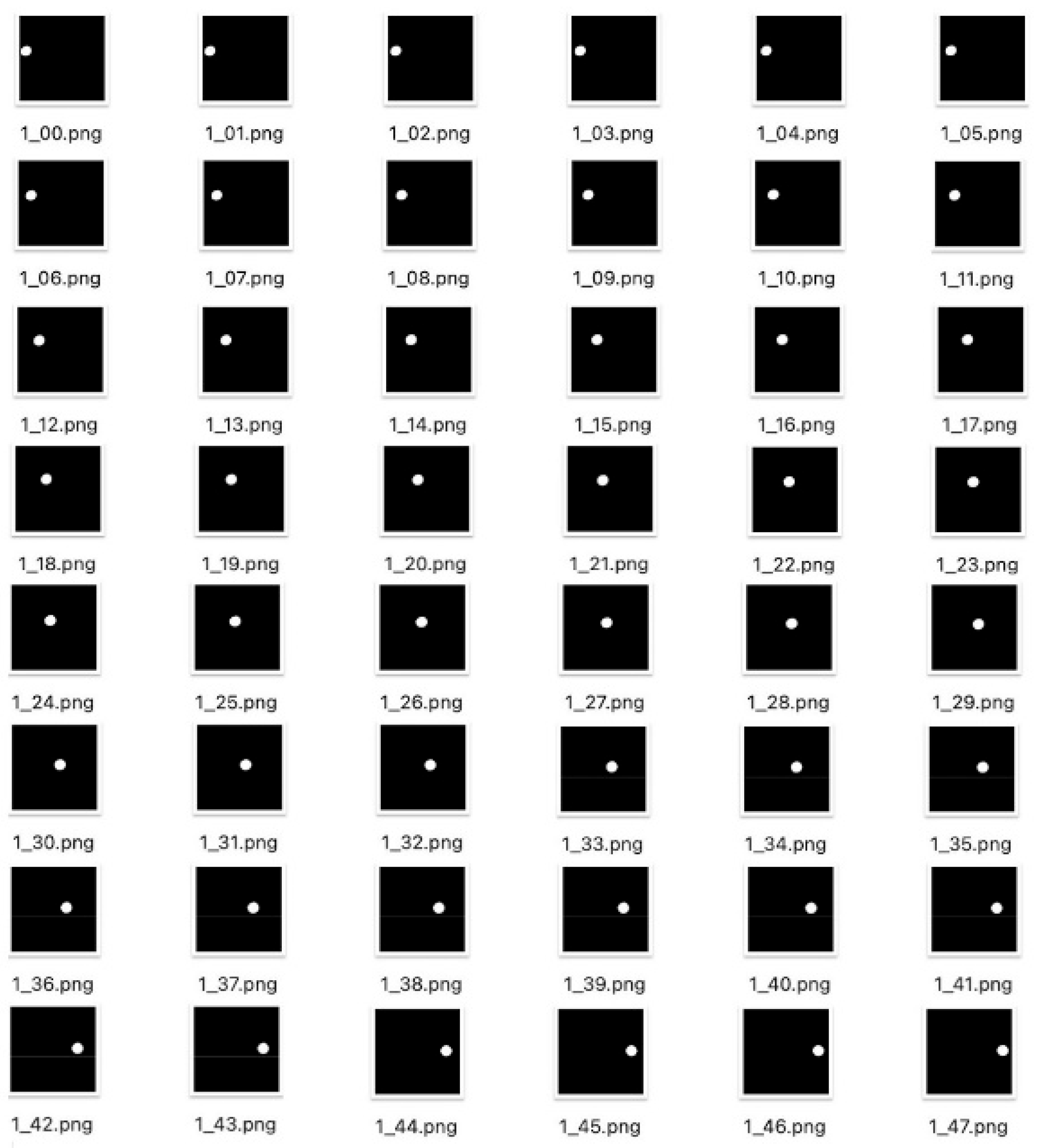
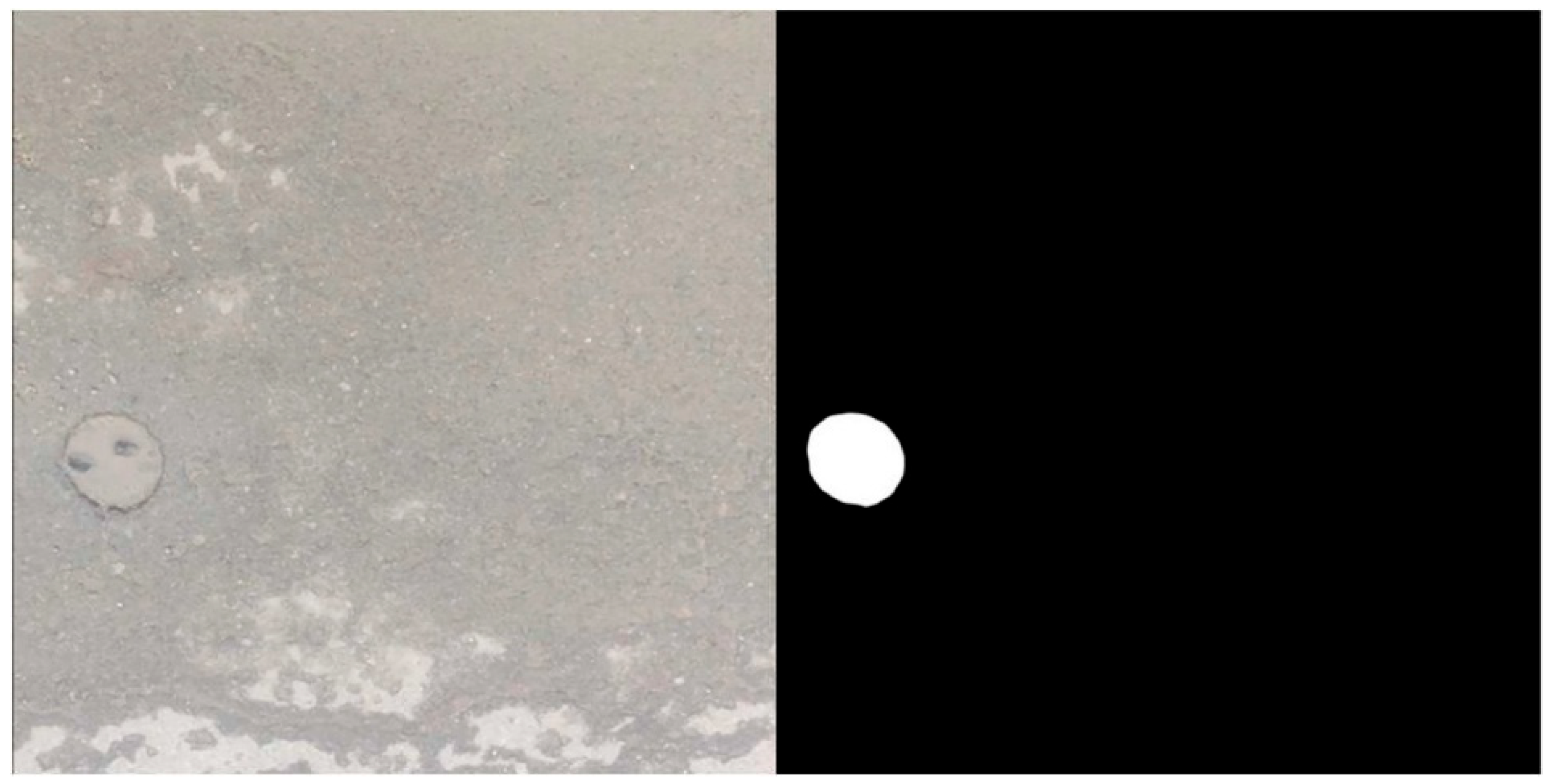
The subsequent sections of this work are structured as follows. Section 2 examines pertinent literature on pothole detection, whereas Section 3 discusses the utilized novel video dataset. Section 4 outlines the methodology for the deployed models. Section 5 present the experimental results and discussion, while Section 6 concludes the study.

Extensive research exists on pothole identification, encompassing both conventional machine learning methods and deep learning methodologies. Conventional machine learning techniques, including Otsu’s thresholding [18], spectral clustering [19], morphological operations and other various techniques [20,21,22] are employed to delineate and identify prospective pothole areas. Although these methods offer reduced processing demands, their classification efficacy and robustness are frequently constrained. Certain research utilize 3D point cloud data, using surface normal information for the geometric modeling of potholes [23,24]. Nonetheless, the gathering of 3D point cloud data is frequently expensive and resource-intensive. Currently, the swift advancement of deep learning technologies has led to the proposal of several CNN-based networks for object detection, hence generating substantial prospects for the advancement of pothole detection. These approaches substantially improve the accuracy and reliability of pothole detection, with exact location of potholes achieved [25,26]. The one-stage method You Only Look Once (YOLO) [27,28] is widely utilized in pothole identification because to its superior accuracy and real-time processing capabilities. Ukhwah et al. [29] illustrated the efficacy of YOLOv3 and its variants in detecting road potholes. Shaghouri et al. [30] presented CSPDarknet53 as a backbone derived from YOLOv4, attaining an equilibrium between precision and velocity. Mahalingesh et al. [31] combined the YOLOv8 algorithm and implements it on a Raspberry Pi for hardware evaluation, underscoring the considerable potential of YOLO-based algorithms in practical applications [32,33,34,35,36,37].

2. The Integration of Industry 4.0 with Road Inspection

The historical foundation of road infrastructure management has been built upon manual inspection techniques and reactive maintenance protocols, which have dominated the field for much of the 20th century and into the early 21st [38]. These traditional approaches center on human-led visual evaluations, often guided by established standards such as the Pavement Condition Index (PCI), a quantitative metric developed by the U.S. Army Corps of Engineers that aggregates distress manifestations like alligator cracking, longitudinal cracking, transverse cracking, block cracking, patching, potholes, rutting, raveling, and shoving [39,40]. Inspectors, typically civil engineers or trained technicians, conduct on-site assessments using handheld tools including crack gauges for measuring crack widths, laser profilometers for quantifying rut depths, and falling weight deflectometers (FWD) for non-destructive evaluation of pavement structural capacity, though the latter is less common in routine manual surveys due to its equipment-intensive nature [41].

In practice, manual crack mapping involves delineating distress patterns on scaled drawings or digital tablets, categorizing them by type, severity, and extent [42]. Ride quality assessments incorporate the International Roughness Index (IRI), derived from vehicle-mounted accelerometers or manual straightedge methods, where surface deviations are logged to estimate user comfort and vehicle wear [43]. These data streams are then inputted into Asset Management Systems (AMS), which employ decision trees or priority matrices to rank maintenance needs based on factors like traffic volume, measured in Average Annual Daily Traffic (AADT), and asset criticality. However, the labor-intensive nature of these inspections poses significant challenges. Comprehensive surveys of urban road networks can require teams of 4–6 personnel per segment, with costs escalating to $200–500 per kilometer when factoring in traffic control measures like lane closures and safety barriers [44]. Inter-observer variability is well-documented in literature, with studies indicating discrepancies in distress ratings as high as 25% between inspectors, attributed to subjective interpretations influenced by lighting conditions, weather, or personal experience levels [45]. Moreover, the episodic frequency of inspections often annual or biennial creates temporal gaps, failing to capture acute degradation events such as those precipitated by heavy rainfall leading to water ponding and subsequent asphalt stripping, or freeze–thaw cycles causing expansive damage in bituminous layers [46].

Traditional maintenance strategies exacerbate these limitations by adopting a predominantly reactive stance. Interventions are triggered by threshold breaches in PCI scores or public complaints, leading to spot repairs like pothole filling with hot-mix asphalt (HMA) or cold-patch materials, crack sealing with polymer-modified emulsions, or full-depth patching for severe structural failures [47]. Calendar-based scheduling, such as biennial slurry seals or 10-year overlays, disregards real-time condition variability, resulting in either over-maintenance or under-maintenance. For instance, untreated potholes can evolve from surface depressions to subgrade voids, increasing repair costs by factors of 5–10 compared to early interventions [48]. This revolution is characterized by nine foundational pillars: big data and analytics, autonomous robots, simulation, horizontal and vertical system integration, the internet of things, cybersecurity, the cloud, additive manufacturing, and augmented reality [49].

Safety concerns are paramount, as inspectors operating in live traffic environments face risks from vehicular collisions, with reported incident rates in some jurisdictions exceeding 5 per 1000 inspections. Environmental inefficiencies also arise, with reactive repairs generating excess waste from milled materials and higher embodied carbon from frequent heavy machinery deployment. Literature critiques these methods for their inability to integrate multifaceted stressors, including escalating traffic loads, climate-induced accelerations in deterioration, and societal demands for minimal disruptions. As global road networks age with over 40% of U.S. pavements classified as fair or poor traditional practices prove increasingly untenable, necessitating a shift toward digitized, proactive paradigms [13,14].

Industry 4.0, originating from Germany’s high-tech strategy in 2011 and expanding globally, signifies the integration of cyber–physical systems (CPS) with advanced digital technologies to revolutionize industrial processes, extending its influence to civil infrastructure domains like road management. In transportation contexts, these technologies converge to transform static road assets into dynamic, interconnected ecosystems capable of real-time responsiveness and predictive optimization [50].

Central to this is IoT, deploying networks of sensors such as fiber Bragg grating (FBG) strain sensors with wavelength-shift detection for micro-strain monitoring, or wireless accelerometers operating on Zigbee protocols for vibration analysis to generate voluminous data streams [51]. Big data analytics, powered by frameworks like Apache Hadoop for distributed storage and Spark for in-memory processing, handle petabyte-scale datasets, employing techniques such as principal component analysis (PCA) for dimensionality reduction and k-means clustering for pattern identification in distress evolution [52]. Cloud computing platforms facilitate scalable storage and collaborative access, while edge computing via devices modules enables localized inference, reducing latency to milliseconds for time-sensitive applications [53]. Artificial intelligence and machine learning algorithms underpin predictive capabilities, with supervised models like random forests classifying distress types from sensor inputs, and deep learning architectures processing multimodal data. Cybersecurity measures, such as blockchain-ledgered data integrity checks using hashing, protect against tampering in shared networks. Additive manufacturing supports on-site repairs with 3D-printed patches from geopolymer materials, enhancing sustainability [54,55]. Augmented reality (AR) aids field technicians via head-mounted displays overlaying digital twins onto physical assets for guided interventions [56].

In road infrastructure, these technologies address systemic pressures: IoT-enabled continuous monitoring detects early microcracks invisible to manual inspections, big data correlates deterioration with exogenous variables like salinity from de-icing salts, and AI forecasts failure probabilities [57]. Literature highlights efficiency gains, with Industry 4.0 implementations reducing maintenance costs through optimized resource allocation and extending asset lifespans via proactive strategies. Sustainability benefits include minimized material usage and lower emissions from fewer site visits. This technological suite sets the stage for specialized applications in road inspection and maintenance, fostering resilience in the face of urbanization and climate change [58], This literature also connects strongly with established quality control theories in manufacturing processes, particularly statistical quality control (SQC) and stochastic process monitoring. In traditional manufacturing systems, variability is treated as an inherent stochastic behavior of the process, and quality assurance is achieved through continuous monitoring, sampling strategies, and control mechanisms that detect deviations before they propagate into system-level failures. Industry 4.0 extends this paradigm by embedding sensing, automation, and data-driven analytics into the inspection loop, enabling real-time quality assessment under uncertainty. In this context, road infrastructure inspection can be interpreted as a stochastic quality control problem, where defects such as potholes, cracks, and surface degradation evolve under highly variable environmental and operational conditions [59]. Similar to manufacturing systems operating under noise and uncertainty, road surfaces exhibit non-deterministic deterioration patterns influenced by traffic load, weather fluctuations, and material heterogeneity. The adoption of Industry 4.0 technologies therefore enables a shift from periodic inspection to continuous, data-driven quality monitoring, aligning infrastructure assessment with modern stochastic quality control frameworks [60].

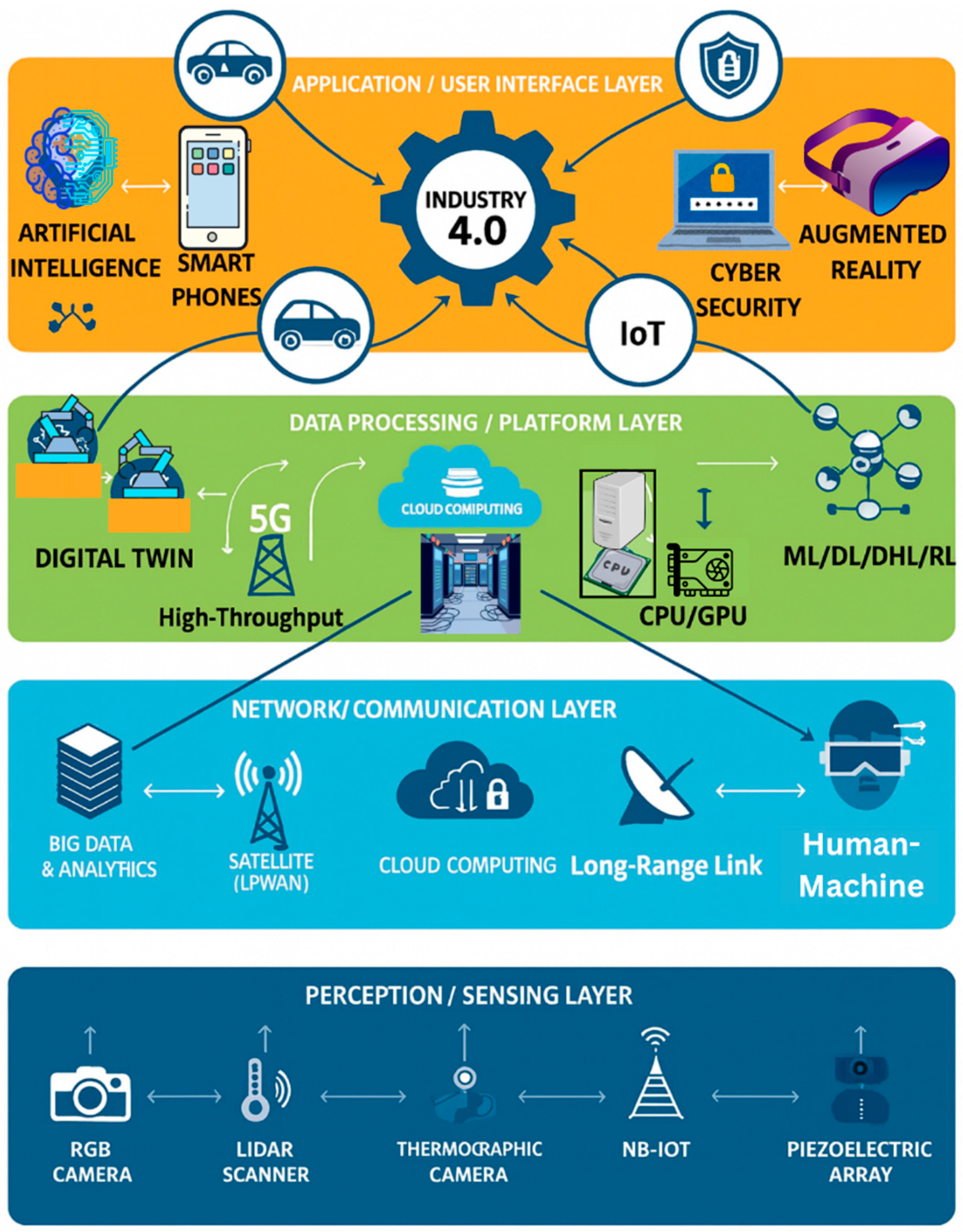
In the context of smart road inspection and maintenance, IoT architectures are commonly structured as a multi-layered system to ensure scalable data acquisition, reliable communication, and intelligent decision-making. At the lowest level, the perception or sensing layer comprises heterogeneous sensors, including RGB cameras, LiDAR scanners, thermographic cameras, piezoelectric arrays, and NB-IoT devices, which continuously capture surface and subsurface pavement conditions such as cracks, potholes, rutting, vibration, and thermal anomalies [61]. Sensor data are transmitted through the network and communication layer, which integrates short- and long-range technologies (e.g., LPWAN, satellite links, 5G) to enable robust, low-latency data transfer across distributed road networks. The data processing and platform layer aggregates and processes incoming data using cloud and edge computing resources, where big data analytics, digital twins, and AI models execute tasks such as feature extraction, anomaly detection, and degradation forecasting [62]. At the highest level, the application and user interface layer translates processed information into actionable intelligence through dashboards, mobile devices, augmented reality interfaces, and asset management systems, supporting condition-based and predictive maintenance strategies [63]. This layered IoT architecture enables a closed-loop framework for continuous monitoring, automated defect detection, and optimized maintenance decision-making, as illustrated in Figure 1.

Road Inspection 4.0 embodies the application of Industry 4.0 tenets to pavement monitoring, conceptualizing roads as cyber–physical systems (CPS) that fuse physical elements such as asphalt concrete or other types of pavements with digital overlays for autonomous, continuous assessment [45]. This paradigm deploys a multilayered architecture that starts with the perception layer with heterogeneous sensors including piezoelectric vibration sensors for dynamic load responses, thermographic cameras for heat signature-based crack detection, and LiDAR scanners for 3D surface profiling at sub-millimeter accuracy. The network layer utilizing 5G for high-throughput data transfer and NB-IoT for energy-efficient, long-range connectivity in rural segments. The application layer integrating digital twins via virtual simulations of stress distributions under varying traffic scenarios [64]. Continuous Monitoring Systems (CMS) in Inspection 4.0 supplant traditional snapshots with streaming data, enabling real-time anomaly detection through algorithms like isolation forests for outlier identification in sensor readings. Vision-based modalities dominate, with fixed cameras employing high-dynamic-range (HDR) imaging to handle varying illuminance, processed at the edge using Tensor Processing Units (TPUs) for inference acceleration [65].

Maintenance 4.0 evolves this further by adopting Condition-Based Maintenance (CBM) and Predictive Maintenance (PdM). CBM monitors key performance indicators like deflection ratios from embedded strain gauges, triggering alerts when thresholds are exceeded. PdM leverages prognostic models, such as survival analysis with cox proportional hazards, to estimate time-to-failure based on historical trends and environmental covariates [66]. Risk-based prioritization uses multi-criteria decision analysis tools like Analytic Hierarchy Process (AHP) to balance cost, safety, and disruption. Distinctions from traditional methods are profound. Where manual inspections incur high variability and costs, Inspection 4.0 achieves higher consistency via automated analytics, with operational expenses reduced through remote sensing. Temporal resolution improves from annual to continuous, capturing transient events like load-induced fatigue. Maintenance 4.0 minimizes reactive repairs, which account for 60–70% of traditional budgets, by enabling just-in-time interventions that extend pavement. Scientific rationale lies in preventing exponential distress growth, as early detection halts mechanisms like moisture ingress leading to base erosion [67].

Artificial intelligence catalyzes the efficacy of Inspection and Maintenance 4.0 by processing complex, high-dimensional data into precise, actionable insights, surpassing human capabilities in speed, scalability, and objectivity. AI frameworks encompass a spectrum of techniques: supervised learning for labeled distress classification, where models like Gradient Boosting Machines (GBM) achieve high recall in identifying rare events; unsupervised learning for novelty detection, utilizing variational autoencoders (VAEs) to reconstruct normal pavement states and flag deviations; and reinforcement learning (RL) for optimizing maintenance schedules, with Q-learning algorithms maximizing rewards based on cost minimization and service level maximization. Time-series analysis employs recurrent architectures like Gated Recurrent Units (GRUs) to model sequential sensor data, capturing temporal dependencies in deterioration patterns influenced by cyclic loading. Ensemble methods, combining bagging and boosting, enhance robustness against noisy inputs from real-world environments. CNNs are particularly emphasized for their prowess in vision-based tasks, extracting spatial hierarchies through convolutional kernels, batch normalization for training stability, and dropout for overfitting prevention [68]. Prominent architectures include YOLO variants for real-time bounding box prediction [68,69,70].

Pothole detection serves as a prime use case for Inspection 4.0, employing AI-centric vision systems for automated identification and characterization. Deployment involves roadside or vehicle-mounted RGB cameras capturing pavement imagery, preprocessed with techniques like histogram equalization for contrast enhancement and Gaussian blurring for noise reduction. CNN models applications can be traced to almost all industries. Edge-deployed CNNs, optimized for low-power hardware, perform inference to output bounding boxes, class probabilities, and confidence scores, with post-processing via non-maximum suppression (NMS) to eliminate redundant detections [71].

Data augmentation rotations, flips, brightness adjustments mitigates overfitting, while federated learning allows model updates across distributed agencies without data sharing. Post-detection, Maintenance 4.0 utilizes AI for recommendation issuance: severity classification via multi-head CNNs estimating depth and area, then feeding into rule-based or ML-driven systems for suggestions. Integration with GIS platforms like ArcGIS overlays detections on maps, prioritizing based on traffic density and proximity to critical infrastructure. Drones (UAVs) enhance accessibility, with quadcopters equipped with 4K cameras and RTK GPS for georeferenced orthophotos. AI processing on drone payloads or ground stations uses Mask R-CNN for instance segmentation. Swarm drone operations cover large areas efficiently, fusing data with ground sensors for validation [72].

Despite promising advancements, challenges hinder widespread deployment of Inspection 4.0 and Maintenance 4.0. Sensor durability against environmental aggressors like UV degradation of camera lenses or corrosion of embedded gauges in saline conditions requires advanced materials such as epoxy-encapsulated units. Data quality issues, including sensor drift and biases in AI training datasets, compromise model reliability, with studies noting drops in accuracy under adverse weather. Upfront investments pose barriers, necessitating ROI demonstrations through lifecycle analyses showing 20-year paybacks. Interoperability across vendors demands open standards for seamless integration. Cybersecurity vulnerabilities, such as DDoS attacks on cloud platforms, require robust encryption and anomaly detection. Human factors include workforce reskilling for AI literacy and regulatory hurdles in data privacy [73]. Future trajectories emphasize enhanced multimodal fusion, combining vision with vibro-acoustic data via attention mechanisms in transformers for holistic diagnostics [74]. Explainable AI (XAI) techniques will build trust in black-box models. Large-scale field trials, such as those in low-light conditions using thermal imaging, aim for validation across climates. Advancements in edge AI with quantized models will enable ultra-low latency on resource-constrained devices. Sustainability focus includes energy-harvesting sensors via piezoelectric pavements. Policy advocacy for standardized architectures will accelerate adoption, positioning these paradigms as cornerstones for resilient transportation [75].

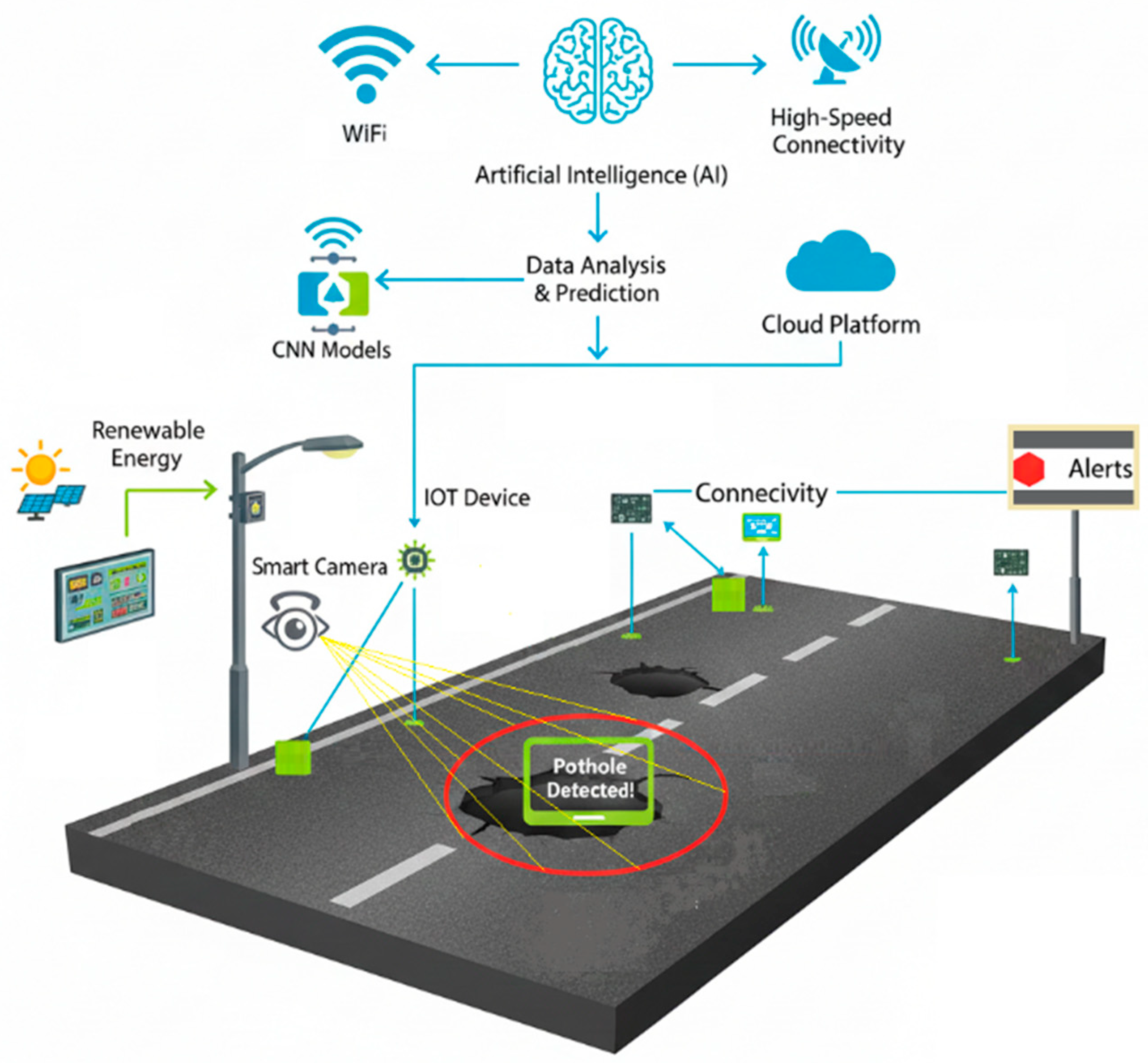
A seamless pothole detection framework for smart road inspection integrates distributed sensing, edge intelligence, cloud-based analytics, and real-time communication into a unified cyber–physical system [76]. At the perception layer, smart roadside cameras powered by renewable energy sources and co-located with auxiliary sensors continuously capture high-resolution visual data of the pavement surface. These sensing units are equipped with embedded IoT devices that enable local preprocessing and reliable data transmission via wireless connectivity. CNN models deployed either at the edge or in the cloud perform automated feature extraction and inference, enabling robust identification of potholes under varying illumination, traffic, and environmental conditions. The integration of edge inference reduces latency and bandwidth requirements, while cloud platforms support large-scale data aggregation, model retraining, and long-term performance monitoring. Beyond detection, the framework supports real-time situational awareness and actionable response through intelligent communication and alerting mechanisms. Once a pothole is detected and spatially localized, the system propagates this information through high-speed connectivity to cloud platforms and downstream applications [77]. Alerts are issued to roadside display units, asset management systems, or control centers, enabling rapid intervention and prioritization of maintenance activities. This closed-loop architecture ensures continuous monitoring, automated decision support, and timely dissemination of hazard information to both infrastructure operators and road users. By tightly coupling AI-driven analytics with IoT-enabled sensing and communication, the framework enables scalable, resilient, and proactive pothole detection and maintenance workflows, as illustrated in Figure 2.

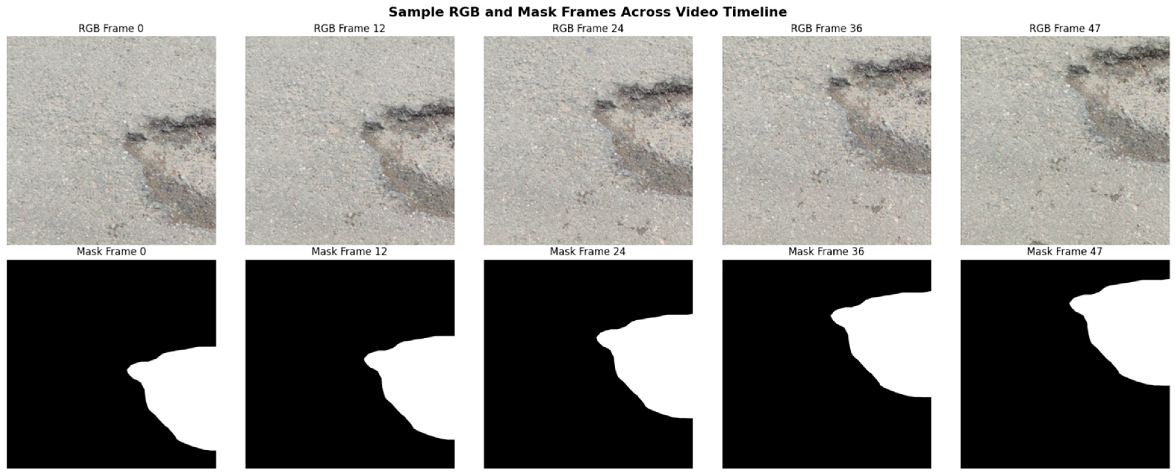
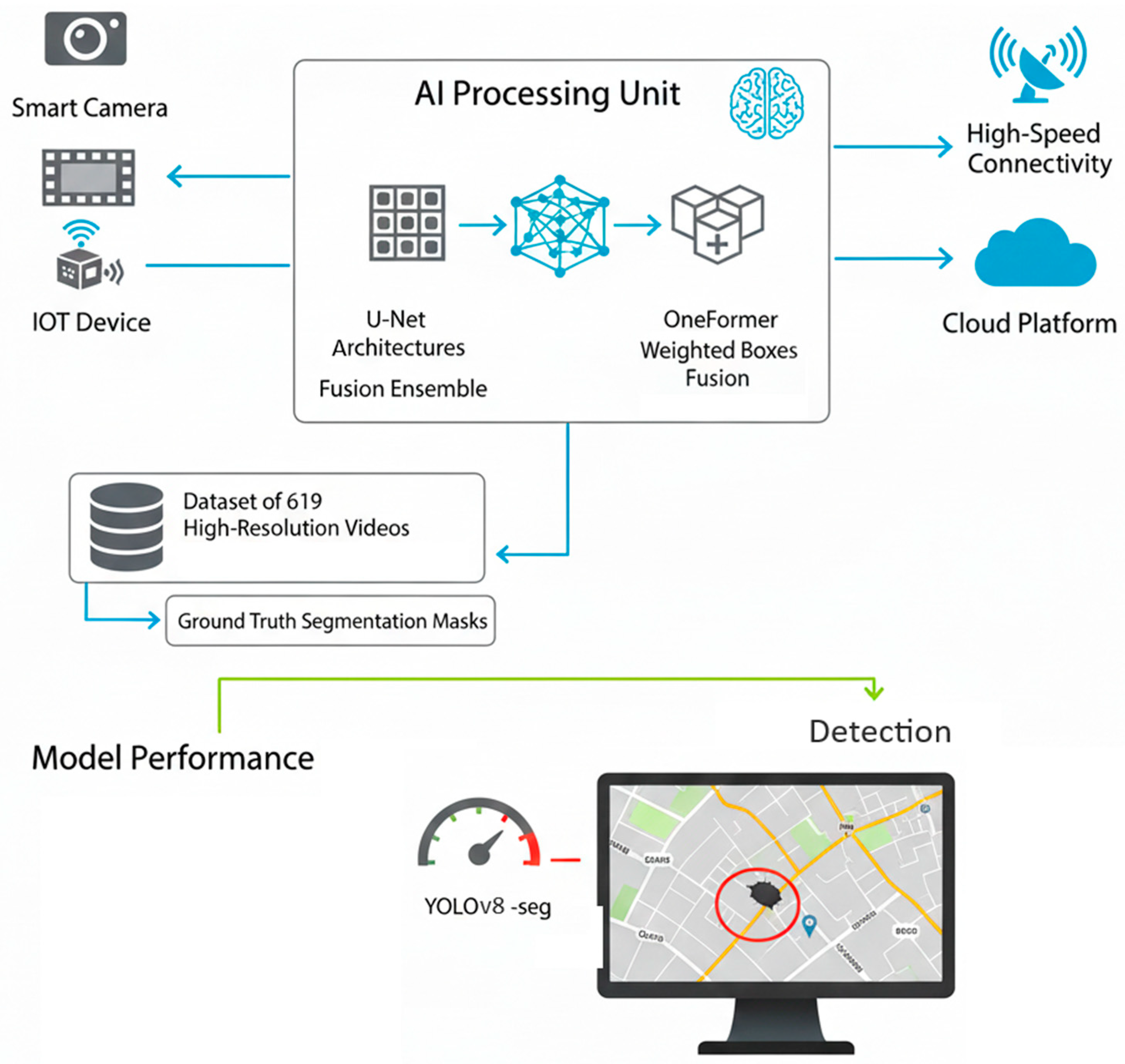
The pothole detection scenario adopted in this study is designed as a fully integrated, video-based AI inference pipeline that combines edge sensing, deep learning–based segmentation, and cloud-assisted analytics. High-resolution video streams are continuously acquired from smart roadside cameras and transmitted via IoT devices to an AI processing unit, where temporal frames are extracted and processed rather than treated as independent images. The learning framework is trained using a curated dataset of 619 high-resolution road inspection videos, accompanied by frame-level ground truth segmentation masks that preserve spatial continuity across consecutive frames. Within the processing unit, multiple U-Net–based segmentation architectures are employed in a fusion ensemble to enhance robustness against illumination changes, motion blur, and occlusions, while OneFormer-based weighted box fusion is used to consolidate predictions and improve spatial consistency of detected potholes. Model performance is evaluated using segmentation-aware metrics and validated through a YOLOv8-seg benchmarking stage, after which geolocated detections are visualized and transmitted through high-speed connectivity to cloud platforms and monitoring interfaces for real-time decision support. This end-to-end video-centric detection workflow is illustrated in Figure 3.

3. A Video-Based Dataset for Pothole Segmentation

This dataset introduces a novel feature that includes moving pothole data captured by a camera. The existing available pothole data mostly consists exclusively of independent and static images [78,79,80,81,82,83]. In this paper, the utilized dataset constitutes a video collection for the semantic segmentation of road potholes.

The dataset comprises 619 high-resolution (2160 × 3840) films recorded in January 2023, encompassing sites in eight villages within the Hulu Sungai Tengah region of South Kalimantan, Indonesia. The dataset is categorized into three primary folders: train, validate, and test. The folders comprise 372 videos for training, 124 movies for validation, and 123 videos for testing, respectively. Each primary folder contains two subfolders: “RGB” for video in RGB format and “mask” for ground truth segmentation. Each movie has a duration of exactly two seconds, has 48 frames, and is formatted in MP4 [84].

The dataset contains a semi-manually annotated ground truth label for each pixel in the video frames, denoting the shape and dimensions of the potholes. The original RGB and ground truth movies each have a constant duration of two seconds, consisting of 48 frames (24 frames per second/fps). Figure 4 presents sample frames from a ground truth movie of this dataset. The white pixels signify potholes, while the black pixels denote non-potholes [84].

The data was gathered from top-down films documenting road potholes, utilizing a Xiaomi Mi10T smartphone camera with a resolution of 2160 × 3840. The distance from the camera to the pothole fluctuated approximately 130 cm based on topography and camera positioning. The pothole is deliberately placed in the upper part of the camera frame to facilitate the pre-processing phase during video capture. Figure 5 shows a representation of data acquisition (left) and the corresponding samples generated (right). Figure 6 illustrates a video frame alongside the corresponding ground truth segmentation [84]. Figure 7 shows sample RGB and mask frames across video timeline.

4. Methodology

The aim of this project is to create a reliable ensemble capable of directly and accurately detecting potholes from real-life video frames. Concerning this purpose, the study commenced by using innovative algorithms on the distinctive dataset of this research and subsequently advanced to the development of the ensemble using a combination of the deployed algorithms. The experiments were conducted on a workstation equipped with an Intel Core i7-10700 CPU (2.90 GHz) and 32 GB RAM (31.7 GB usable). The system runs Windows 11 Enterprise (Version 23H2) on a 64-bit operating system with an x64-based processor.

4.1. Best Frame Selection

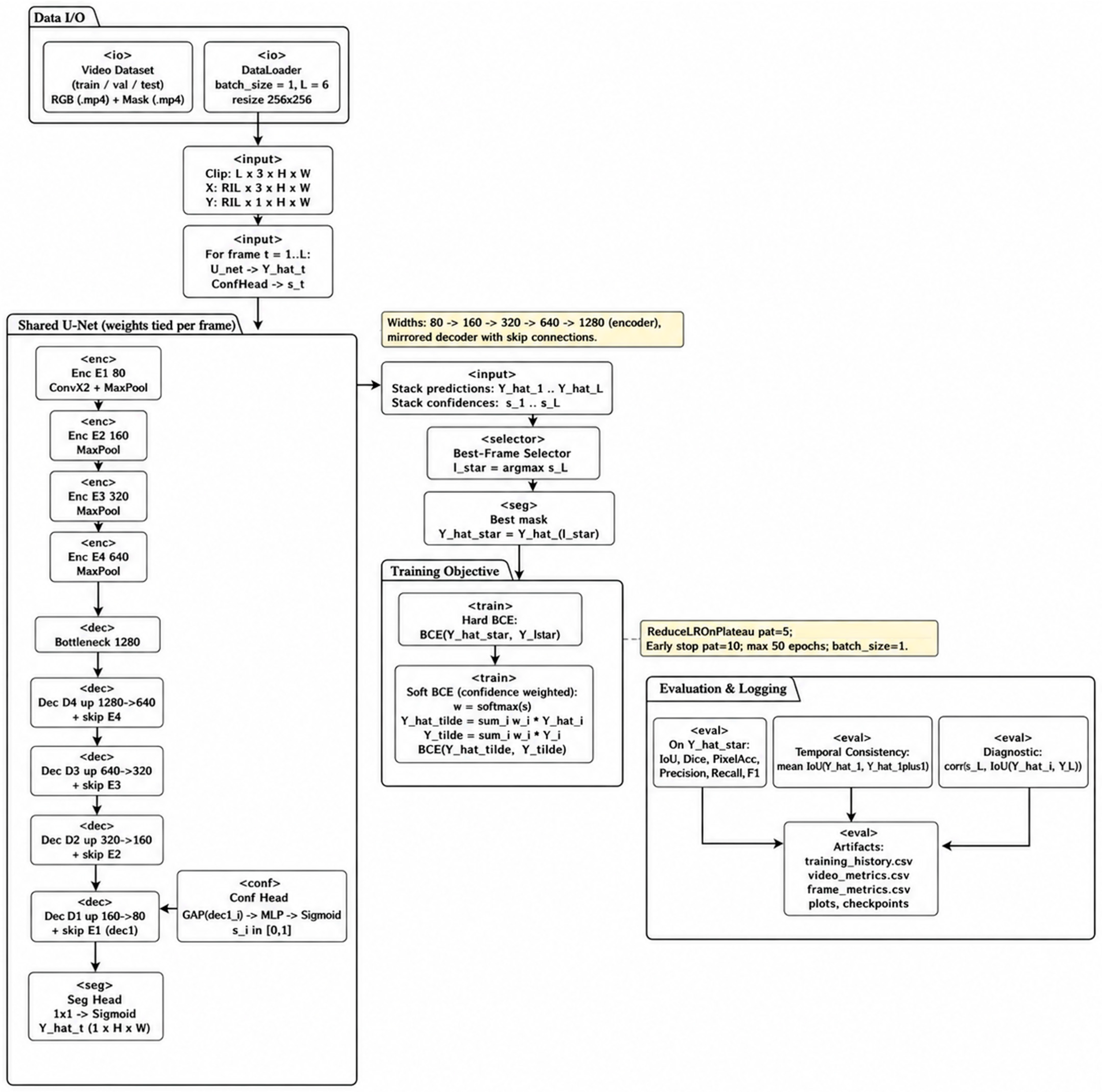
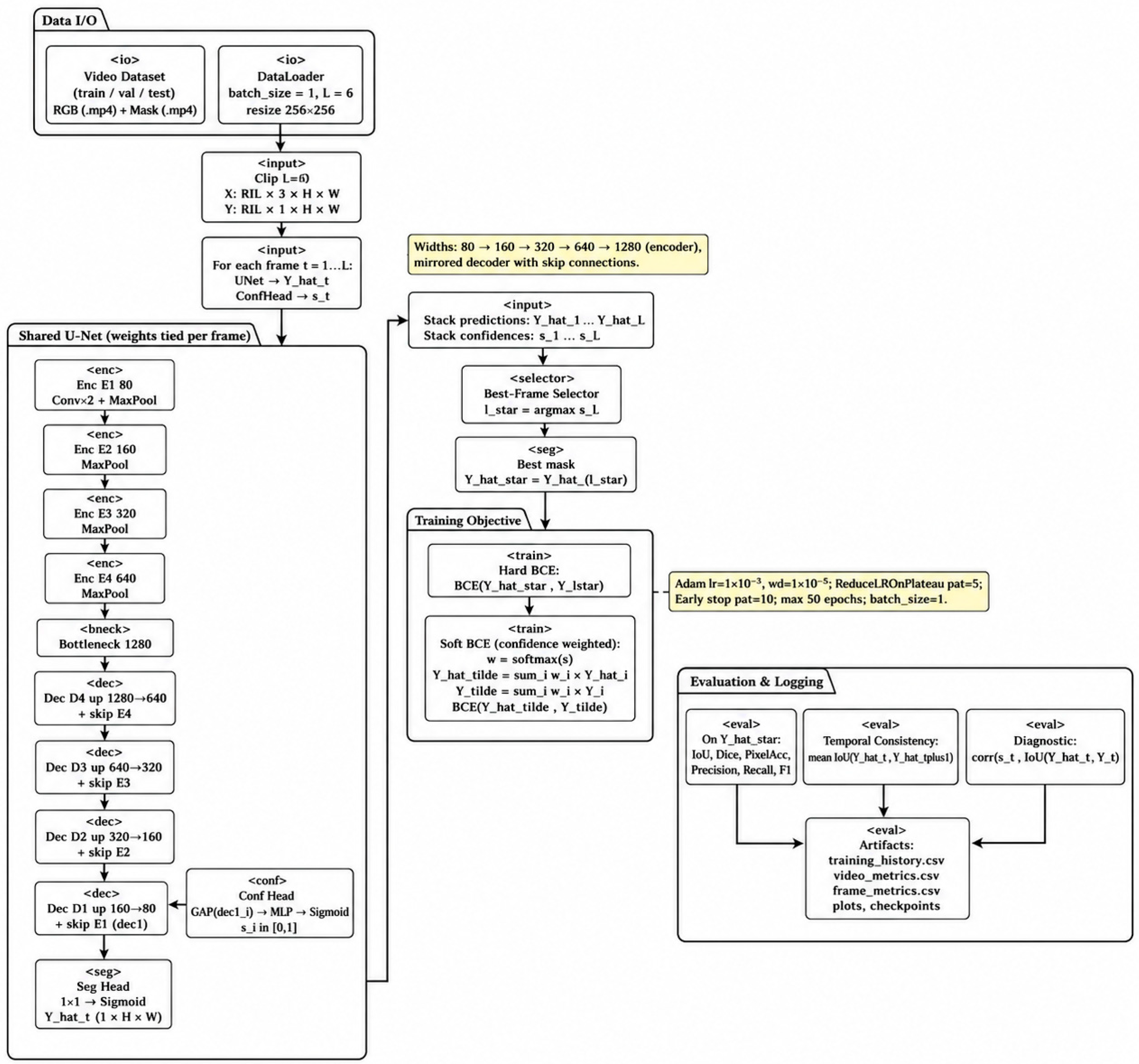
The objective is to segment potholes in video footage while selecting the optimal frames. For each input video, the system extracts a brief sequence of frames, independently predicts a binary pothole mask for each frame, provides a confidence score to every frame, and thereafter selects the single “best” frame (the one with the highest confidence) for reporting and evaluation. The U-Net style encoder–decoder with skip connections follows the established U-Net design [85], It integrates a context-capturing contracting pathway with a precise-localization expanding pathway—a configuration extensively employed in dense prediction challenges and initially developed for biomedical segmentation.

The dataset loader uniformly samples a predefined sequence of 6 frames from each video clip. Each frame is scaled to 256 by 256 pixels. RGB frames are standardized to the range [0, 1]. “Mask videos” are interpreted in grayscale and subsequently thresholded to binary upon resizing. Frames are processed autonomously via the shared U-Net, producing likelihood maps for each frame. Simultaneously, the decoder feature of each frame supplies the confidence head to derive scalar confidence values. The model subsequently determines the index of the optimal frame by applying argmax to the confidence values and returns the probability map of the best frame, the compilation of all per-frame maps, the confidence tensor, and the tensor of the best index. The “predict-all then select-one” methodology is conceptually linked to per-frame video segmentation frameworks that do not explicitly convey temporal information, a method also observed in video object segmentation literature where per-frame segmentations are generated and subsequently stabilized or evaluated retrospectively [86]. After a forward pass on a clip, the system selects the best frame (max confidence). Figure 8 shows the architecture of this algorithm.

4.2. Temporal Consistency Loss Model

The model integrates segmentation and temporal coherence into a unified end-to-end framework. Each frame in a brief clip (sequence length typically six frames) is initially processed through a Full-Size U-Net (encoder widths 80 → 160 → 320 → 640 with a 1280-channel bottleneck and a mirrored decoder with skip connections). The U-Net generates a per-frame logits map that is compressed by a sigmoid function to yield a foreground probability mask. The per-frame predictions are subsequently aggregated along the temporal axis and input into a streamlined temporal refinement module, namely a 3D convolutional head (Conv3D 1 → 16 → 8 → 1 with a 3 × 3 × 3 kernel and a final 1 × 1 × 1 projection). This head enforces local temporal smoothing and facilitates cross-frame information exchange without re-encoding raw RGB sequences, thus maintaining the compactness of the temporal branch while utilizing the high-capacity spatial encoder–decoder [87].

Learning is governed by a three-pronged objective that harmonizes segmentation accuracy and temporal coherence. Initially, a segmentation loss (binary cross-entropy) is calculated for each time step based on both the raw U-Net outputs and the temporally refined outputs, subsequently averaged across the sequence (weight α). Next, a first-order temporal consistency loss employs mean-squared error between refined predictions for consecutive frames to mitigate abrupt temporal variations (weight β). Finally, a second-order smoothness loss penalizes discrepancies in first-order temporal derivatives (i.e., (t − 1 → t) versus (t → t + 1)), thereby diminishing oscillations and promoting smooth dynamics (weight γ). The default weights in the script are α = 1.0, β = 0.5, γ = 0.3, which empirically skews training towards precise masks while still incentivizing temporal regularity. The data pipeline constructs evenly spaced frame subsequences from each video and returns tensors with different shapes for RGB and for masks (256 × 256 resolution by default). Training uses Adam (lr = 5 × 10⁻⁴, weight decay 1 × 10⁻⁴) with Reduce LR On Plateau on validation loss. This approach optimizes the entire clip collectively rather than selecting an individual frame, in contrast to a best-frame selection. The temporal head functions on predictions instead of raw pixels, which (i) stabilizes masks in the presence of noisy appearances, (ii) propagates reliable structures forward and backward across several frames, and (iii) incurs minimal parameter overhead [88]. Figure 9 shows the architecture for this model.

4.3. Multi-Frame Ensemble Model

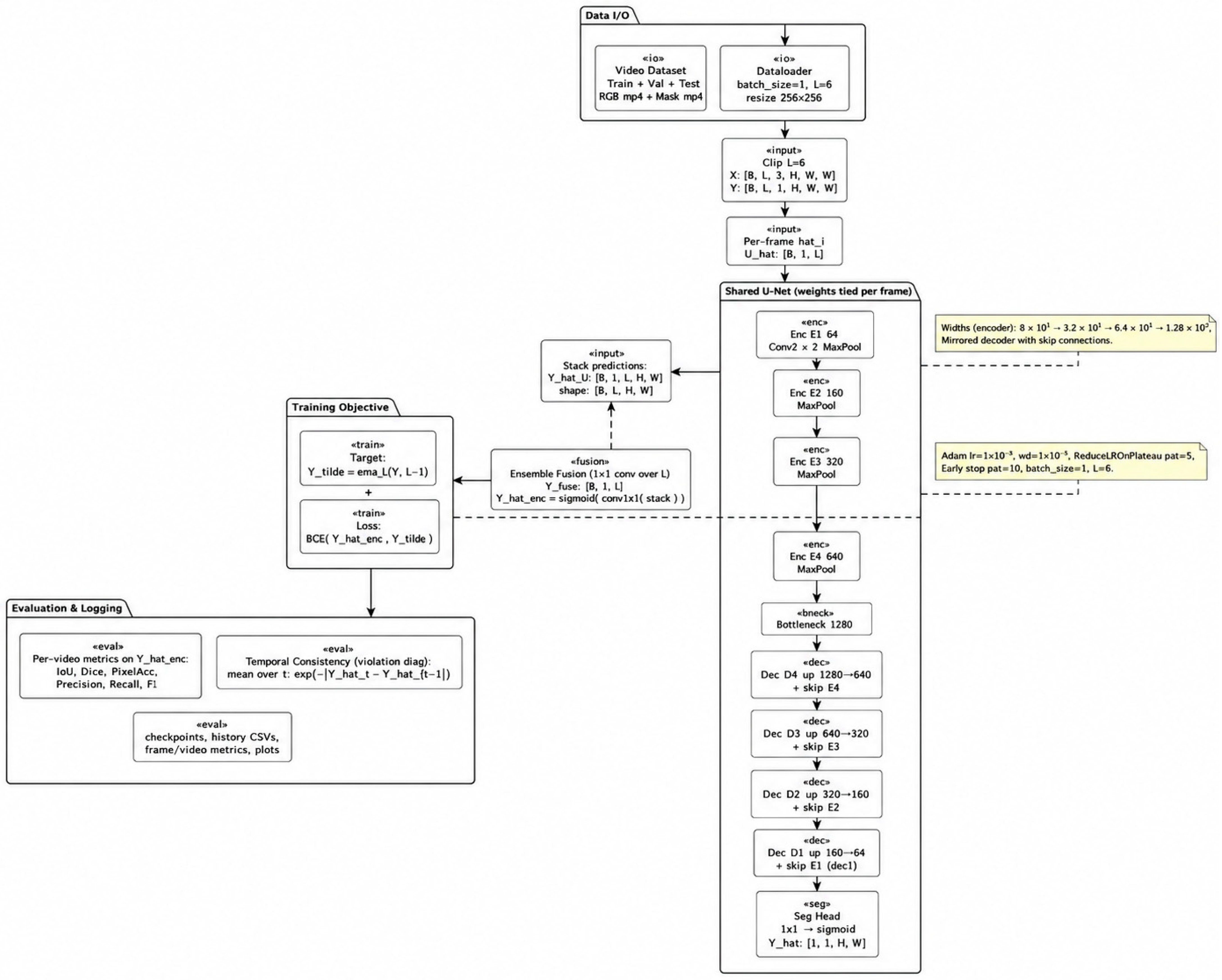
The multi-frame ensemble technique is a per-frame U-Net that consolidates information from a brief clip by layering all frame-specific masks and integrating them using a single 1 × 1 convolution along the temporal axis. Specifically, each frame is processed by a “full-size” U-Net (with encoder widths of 80 → 160 → 320 → 640 → 1280 and a corresponding mirrored decoder); the model generates a sigmoid mask for each frame, aggregates these masks into a tensor and subsequently applies a learnable Conv2d (L → 1, kernel = 1) to produce the ensemble prediction, followed by a sigmoid activation. This system distributes weights across frames without utilizing a recurrent state and incorporates a minimal fusion head, so allocating the majority of capacity to spatial segmentation while the fusion mechanism determines the weighting of frames. The forward path consists of two steps. Step 1 executes the U-Net independently for each frame to generate the ensemble mappings; Step 2 aggregates these mappings along the temporal dimension and conducts 1 × 1 fusion to derive the final mask. The implementation reveals both the fused mask and the individual per-frame masks, which are subsequently utilized for frame-level diagnostics (e.g., temporal consistency).

The training objective is a binary cross-entropy loss on the fused output against a frame-averaged target mask. This choice aligns supervision with the fusion output and removes the requirement to pick a single reference frame, effectively encouraging the fused mask to reflect the agreement across the clip. The method maintains a record of per-frame predictions, allowing evaluation to provide per-video overlap metrics (IoU, Dice) on the ensemble mappings and to calculate a temporal-consistency diagnostic from the frame-wise masks (mean frame-to-frame similarity), thus facilitating a comprehensive assessment of spatial quality and stability.

In contrast to the Best-Frame Selector, the ensemble method circumvents rigid selection and generally achieves superior recall by aggregating data from multiple frames; yet, it is devoid of a learnt ranking signal and may obscure fine details when numerous frames are equivocal. In comparison to the Temporal-Consistency model, the ensemble is less computationally intensive and simpler to optimize, although it provides inferior temporal smoothing, as it integrates data only at the conclusion rather than disseminating information through a temporal convolution/LSTM. Figure 10 shows the architecture for this model.

4.4. OneFormer: One Transformer

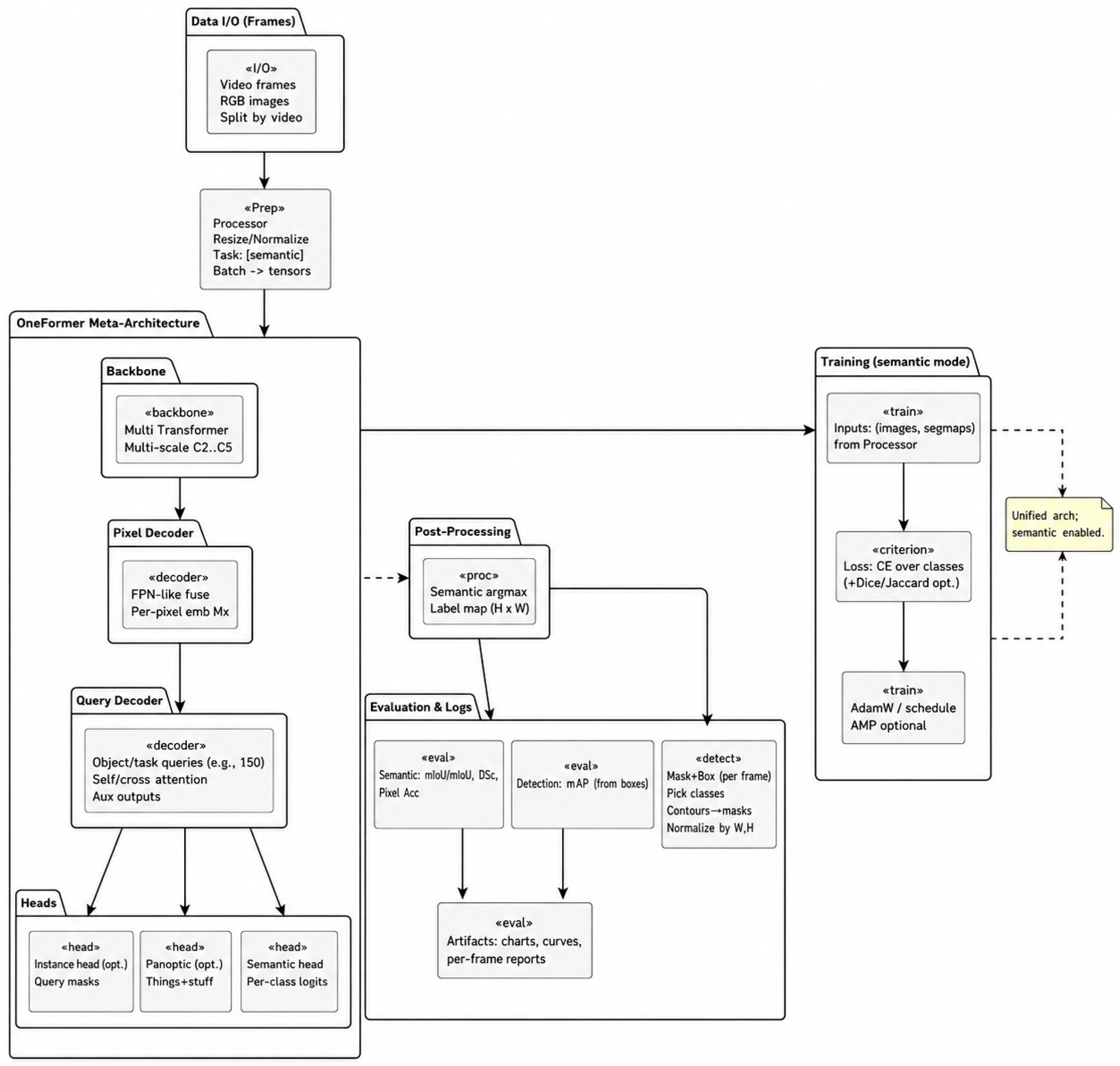
The deployed system is a frame-wise adaption of OneFormer for video data, set in semantic-segmentation mode and utilized as a universal front end for both segmentation and detection tasks [89]. Each video frame undergoes separate processing: an RGB image is normalized and tokenized by the OneFormer processor, thereafter, transmitted to a OneFormer model using a Swin-Transformer backbone that generates dense per-pixel logits. A lightweight pixel decoder consolidates multi-scale characteristics from the backbone, while a query-based transformer head translates them into mask logits based on semantic segmentation cues.

Post-processing transforms the logits into an integer label map at the original image resolution. The implementation generates instance-agnostic proposals by converting class-specific regions in the label map into binary masks and extracting precise, axis-aligned bounding boxes. These boxes are normalized to the image size to facilitate standard detection metrics without the need for training a separate detector. For learning, a fine-tuning pathway generates batches via the OneFormer processor with task_inputs = [“semantic”], and the model is refined using AdamW; evaluation utilizes post-processed predictions to calculate overlap-centric metrics (e.g., IoU) and, when necessary, mean Average Precision from mask-to-box transformations.

The design maintains OneFormer’s cohesive architecture (shared backbone, pixel decoder, and query transformer) while managing temporal aspects externally—frames are processed independently, allowing the same codebase to facilitate pure segmentation, segmentation-to-detection conversion, or later enhancement with external tracking for video-level identity. Figure 11 shows the architecture for this model.

4.5. YOLOv8Seg

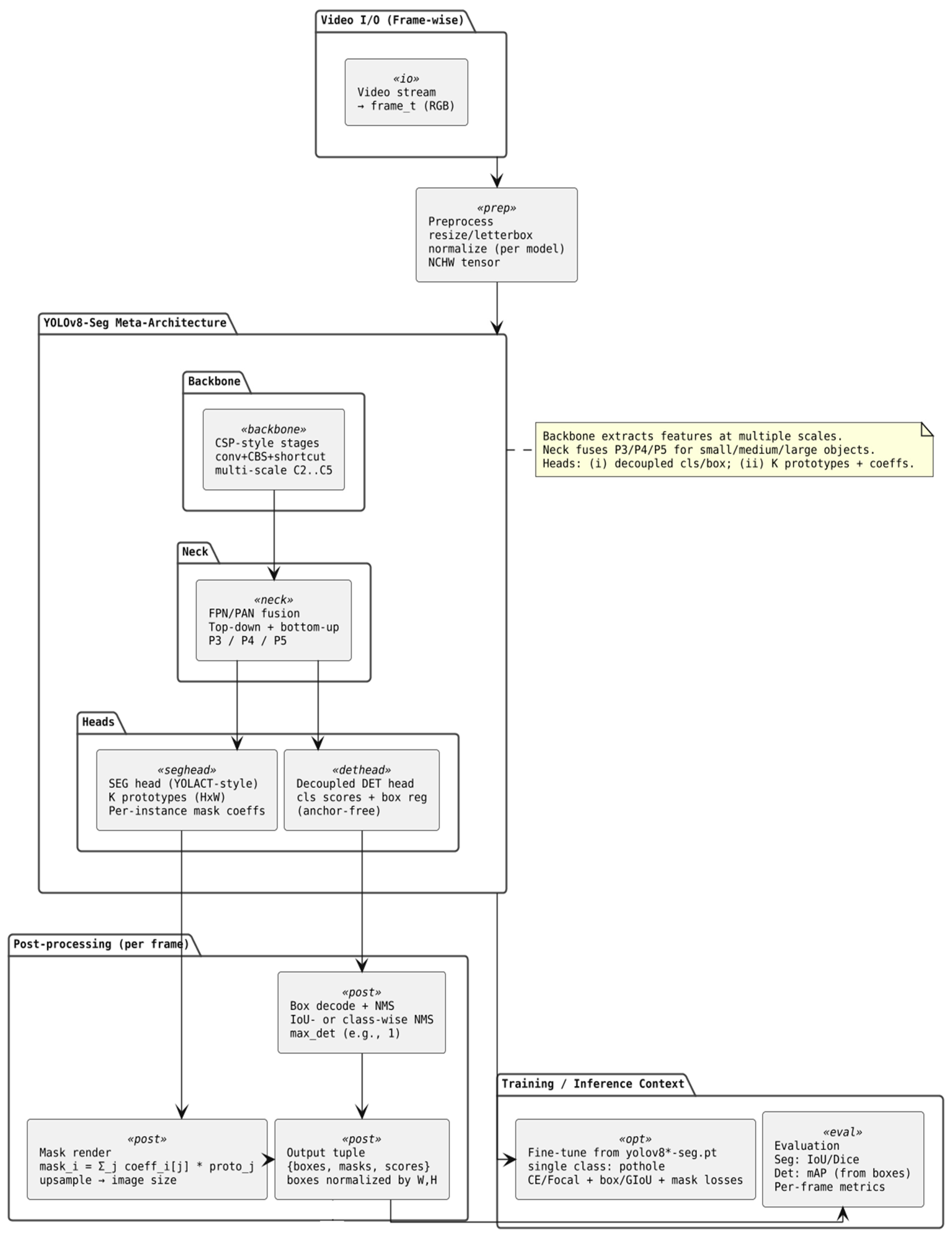
The system uses the YOLOv8 instance-segmentation variation, refining it using a pretrained segmentation checkpoint. Training is performed over 100 epochs with automatic mixed precision deactivated to guarantee numerically stable mask learning on the target data distribution. During inference, each video frame is processed independently by a singular forward pass, producing a triplet: instance masks, bounding boxes, and confidence scores. The implementation restricts the number of returned instances per frame to correspond with the expected sparsity of potholes in road scenes, adjusts the predicted masks to the frame’s native dimensions to preserve geometric accuracy, and normalizes the bounding boxes by image width and height for further evaluation and integration with other modules.

The video pipeline is intentionally frame-centric to maintain the consistency of the segmentation head. Each frame is segmented, masks are enlarged to the original resolution, and boxes are normalized as previously described; confidences are preserved for potential temporal fusion or tracking purposes. This architecture separates spatial learning from temporal logic.

The YOLOv8-Seg model is a single-stage instance segmentation network that enhances the YOLOv8 detector with a streamlined mask head. YOLOv8 utilizes contemporary cross-stage partial connection style residual stages in its backbone to enhance gradient flow and efficiency, incorporating a top-down, multi-scale feature pyramid/aggregation neck to facilitate object detection and segmentation across several scales with minimal additional cost, notions popularized by feature pyramid network and path aggregation network. In addition to these features, a decoupled head forecasts class scores and bounding-box dimensions, while a concurrent segmentation branch generates a predetermined set of prototype masks that are linearly amalgamated with per-instance mask coefficients to produce full-resolution instance masks—an approach influenced by YOLACT that ensures rapid inference while preserving competitive mask quality. Non-maximum suppression is implemented on the bounding boxes, and masks are generated at the image scale for assessment [90]. Figure 12 shows the architecture for this model.

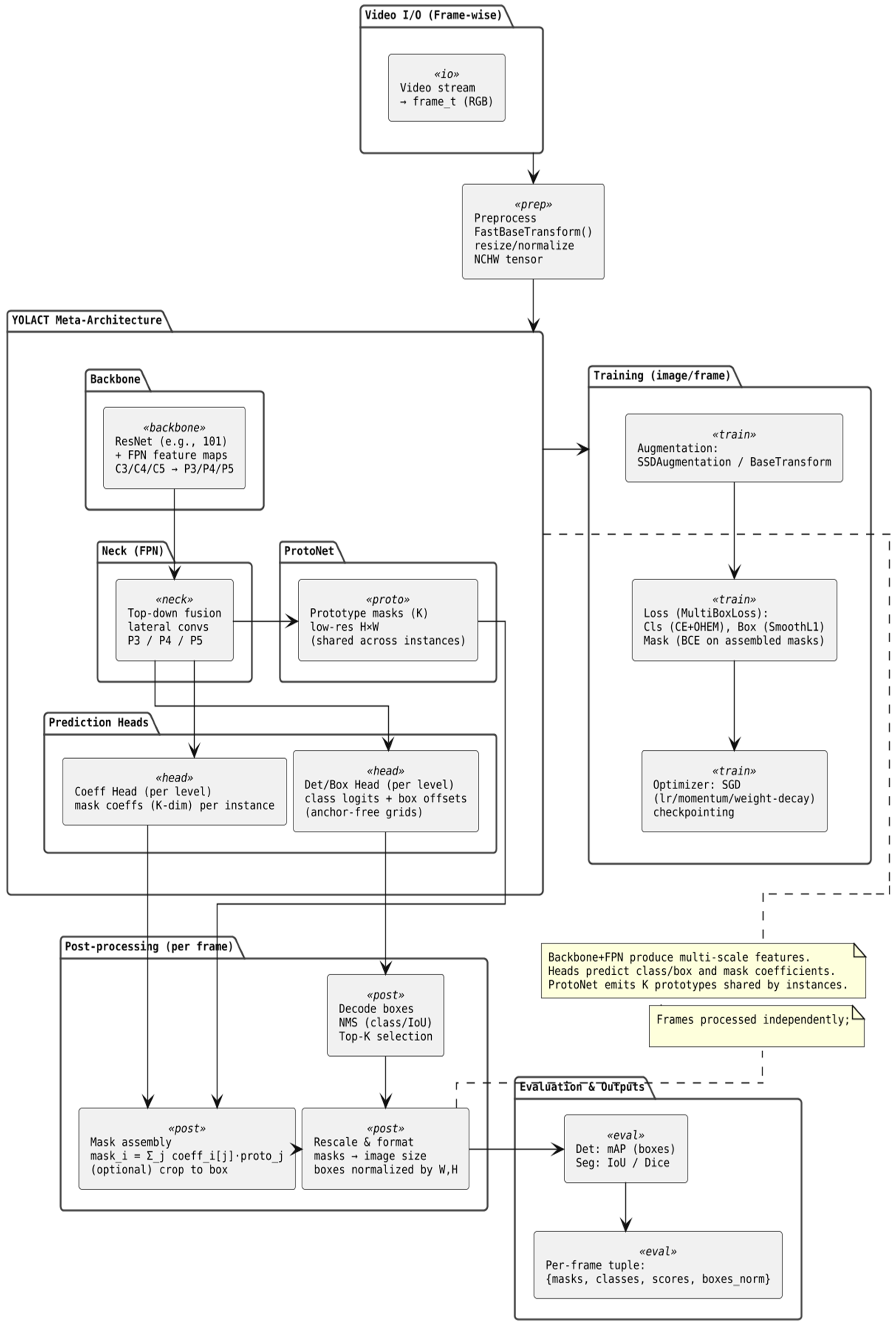
4.6. YOLACT

YOLACT is a single-stage instance-segmentation architecture that separates mask prototype generation from per-instance coefficient prediction, subsequently linearly composing instance masks. This design facilitates rapid video-rate processing while maintaining competitive accuracy, thereby establishing it as a practical baseline for contemporary video segmentation and detection. Recent assessments continue to rank YOLACT among benchmark methods alongside newer detectors and segmenters for the curation of video datasets and baselines, highlighting its significance for swift pixel-level demarcation in dynamic environments [91].

The model training pipeline focused on the original YOLACT architecture and a streamlined inference pathway designed for frame-by-frame video processing. The script establishes a YOLACT network for training and optimizes it using Stochastic Gradient Descent (SGD) with a configuration-driven learning rate, momentum, and weight decay, utilizing COCO-style datasets encapsulated by COCODetection. Data undergo SSDAugmentation for training and BaseTransform for validation, adhering to YOLACT’s standard augmentation protocol. The loss is calculated using MultiBoxLoss, which integrates classification, localization, and mask components with OHEM-style negative mining regulated by positive/negative IoU thresholds and a negpos_ratio. A compact NetLoss wrapper enables effective parallelization by executing the forward pass and loss composition within a single module. CUDA acceleration is activated (cudnn.benchmark = True) when accessible, and model checkpoints/logs are administered by parameters that replicate the original YOLACT scripts. This collectively replicates the conventional YOLACT training protocol while maintaining the configurability of all hyperparameters and dataset connections.

The inference process employs a per-image (per-frame) approach that seamlessly integrates with videos by iterating over frame files. The yolact_model() function initializes a Yolact network, retrieves weights from args.trained_model, transitions to evaluation mode, and, if specified, transfers tensors and the network to CUDA. Each frame is processed using OpenCV, transformed into a tensor, and subsequently transmitted through FastBaseTransform() to generate a batch suitable for the model. The forward pass generates raw detections that are then processed in postprocess(…) (inside final_results_extraction) to derive classes, scores, boxes, and masks, with optional mask cropping and bounding-box rescoring regulated by configuration flags. The code arranges detections based on confidence and yields the top-K results (default K = 5). Masks are retained on the GPU for efficiency; classes, scores, and boxes are transferred to the CPU for subsequent utilization. Ultimately, normalize_bounding_boxes(…) adjusts the bounding boxes to the [0, 1] range by dividing by the image’s width and height.

The model utilizes YOLACT’s prototype-and-coefficients framework for real-time instance segmentation: the model forecasts a collection of global prototype masks and individual instance coefficients; the resultant instance mask is a linear amalgamation of prototypes, which are thresholded and potentially cropped by the predicted bounding box. This renders the method very appropriate for video object detection by independently processing frames with low post-processing burden. Figure 13 shows the architecture for this model. 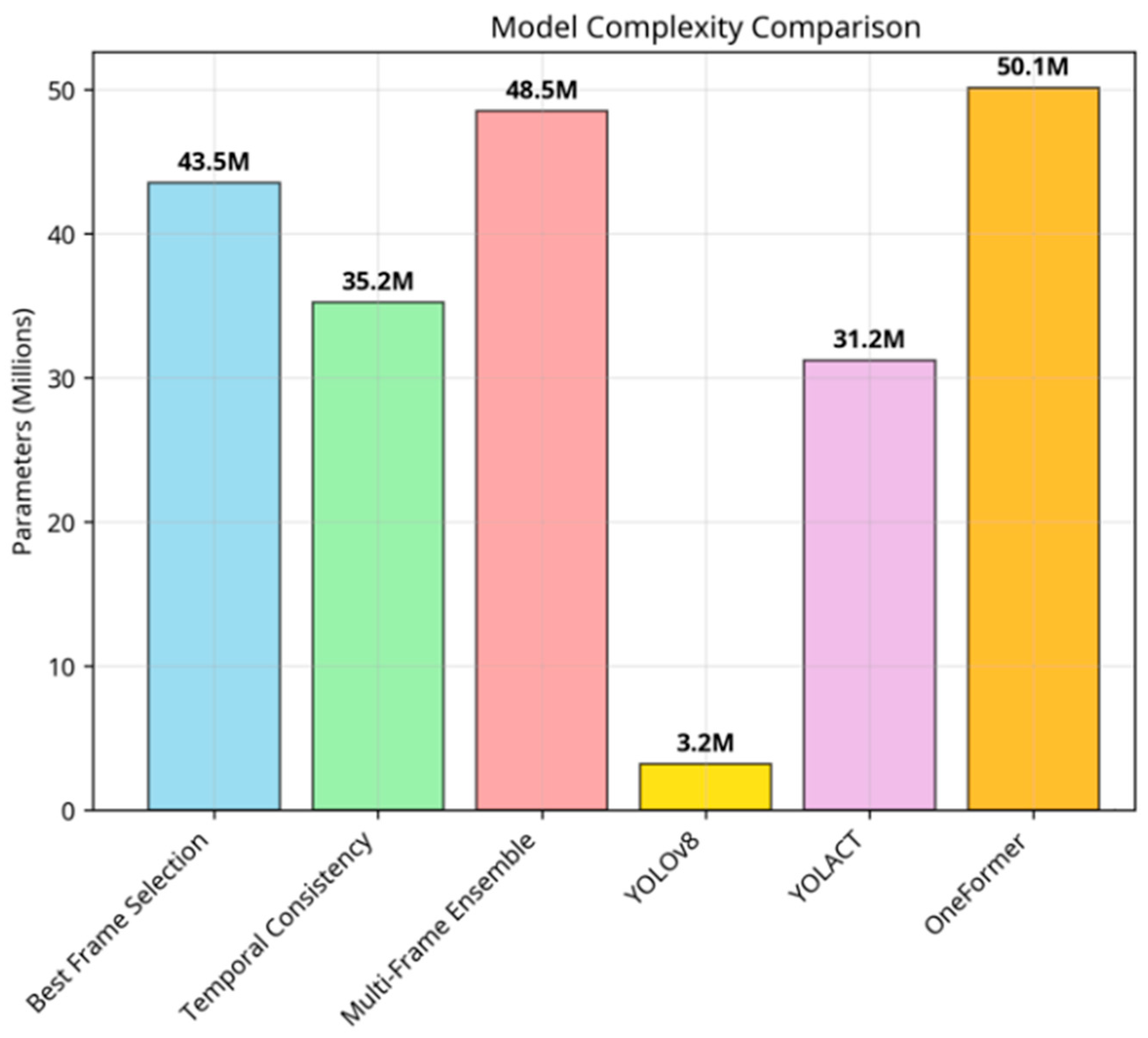Figure 14 shows complexity comparison between the models.

Table 1. Model comparison showing their similarities and differences.

Model	Best Frame Selection	Temporal Consistency Loss	Multi-Frame Ensemble	YOLOv8-Seg	YOLACT	OneFormer
U-Net	x	x	x
YOLOv8n				x
ResNet-101					x
Swin Transformer Tiny						x
Mathematical Fusion Algorithm
6 consecutive frames	x	x	x
Per-Frame				x	x	x
Input Resolution 512 × 512 per frame	x	x	x			x
Input Resolution 550 × 550 per frame					x
Input Resolution 640 × 640 per frame				x
Input Resolution Variable per frame
Adam Optimizer	x	x	x	x		x
SGD with momentum					x
Binary Cross Entropy	x	x	x
Confidence Loss	x
Temporal Consistency Loss		x
Frame Averaging Loss			x
Joint Detection–Segmentation Loss				x	x
Universal Segmentation Loss						x
Better Real-time Capability				x	x	x
High Memory Usage	x	x	x			x

shows a comparison between all the models.

IoU or the Jaccard Index, is a crucial evaluative statistic in computer vision that measures the overlap between two regions or sets. In object detection and segmentation tasks, IoU quantifies the accuracy of a predicted region in relation to the ground truth annotation by computing the ratio of their intersection area to their union area. The metric yields a standardized score ranging from 0 to 1, with 0 signifying no overlap between predicted and actual regions, and 1 denoting complete congruence. This standardization renders IoU especially advantageous for evaluating model performance across various datasets, object dimensions, and detection contexts. The IoU calculation follows a straightforward mathematical formula: IoU = (Area of Intersection/Area of Union) = IoU (A, B) = |A ∩ B|/|A ∪ B|, where

• A represents the predicted region (bounding box or segmentation mask);
• B represents the ground truth region;
• |A ∩ B| is the area of intersection between A and B;
• |A ∪ B| is the area of union of A and B where |A ∪ B| = |A| + |B| − |A ∩ B|.

5. Results and Discussion

5.1. Performance During Training

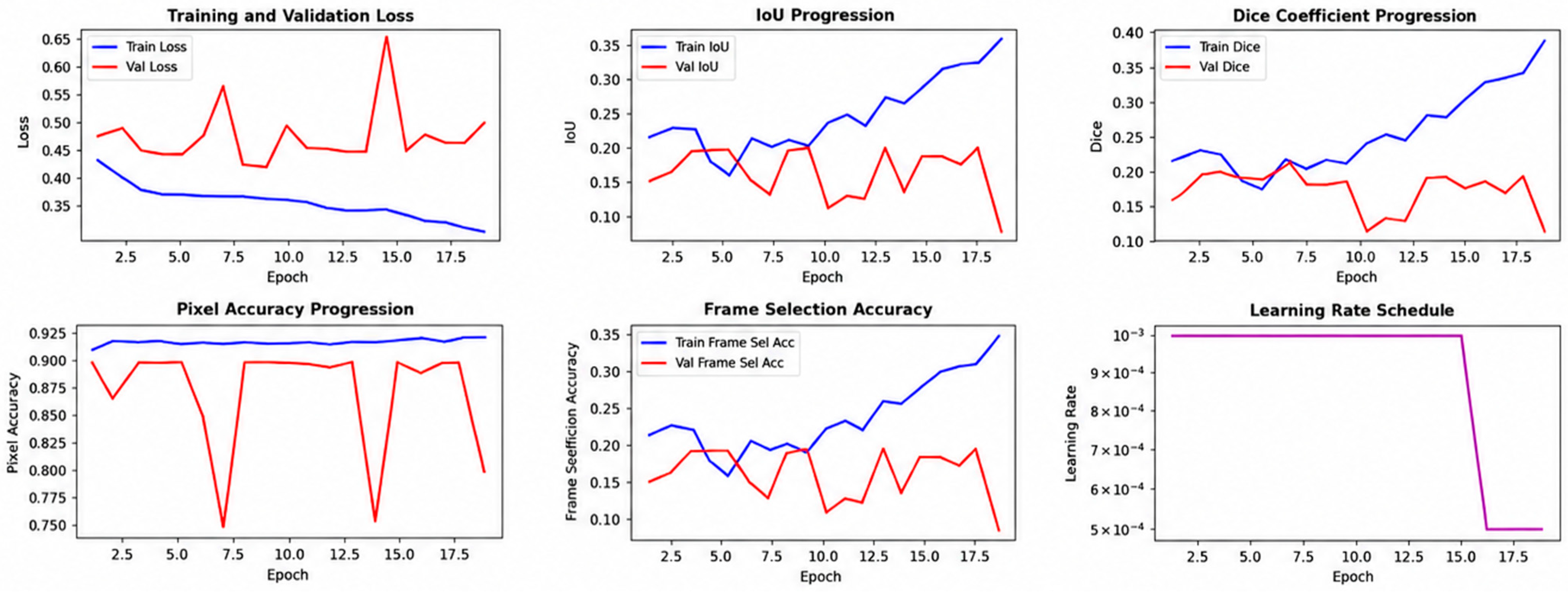
5.1.1. Best Frame Selection Model

The training curves demonstrate that the model reliably learns the training distribution but encounters difficulties in generalization. The training loss consistently declines from the initial epochs to the conclusion of the run, paralleling continuous improvements in the training Intersection over Union (IoU) coefficients. This pattern verifies that the U-Net backbone and the confidence head collectively obtain progressively discriminative features for segmentation and frame-ranking tasks on the observed data.

The validation signals are unstable and relatively feeble. Validation loss demonstrates persistent spikes and a minimal decreasing trend, but validation IoU vary within a limited low range without consistent enhancement. This discrepancy between consistent in-sample advancement and erratic, stagnant out-of-sample performance is indicative of overfitting in high-variance training scenarios. The impact is exacerbated by a batch size of one, resulting in highly stochastic gradients and unstable epoch-level estimates on the validation set.

Pixel accuracy offers a seemingly favorable assessment on both splits, consistently remaining elevated during training and nearing the low-90% range on the training dataset. The simultaneous appearance of elevated accuracy with IoU coefficients during validation strongly indicates class imbalance: background pixels predominate, enabling the model to attain high accuracy while inadequately delineating pothole regions.

The accuracy of frame selection illustrates the matter further. The accuracy of the confidence head in identifying the optimal frame on the training set improves steadily, suggesting a growing correlation between confidence scores and per-frame segmentation quality within the sample. In the validation set, frame-selection accuracy is moderate and fluctuates, suggesting that the acquired rating of frame quality does not consistently apply to previously watched videos. This indicates a discrepancy between the selection target and the supervisory signal accessible during training. The learning rate schedule functions as anticipated at 1 × 10⁻³ until the plateau in validation loss prompts a decrease to 5 × 10⁻⁴. The reduction limits the step size but does not significantly enhance validation IoU, suggesting that the primary constraint is not optimization instability, but rather the generalization gap caused by model’s capacity. Figure 15 shows the model performance during the training process.

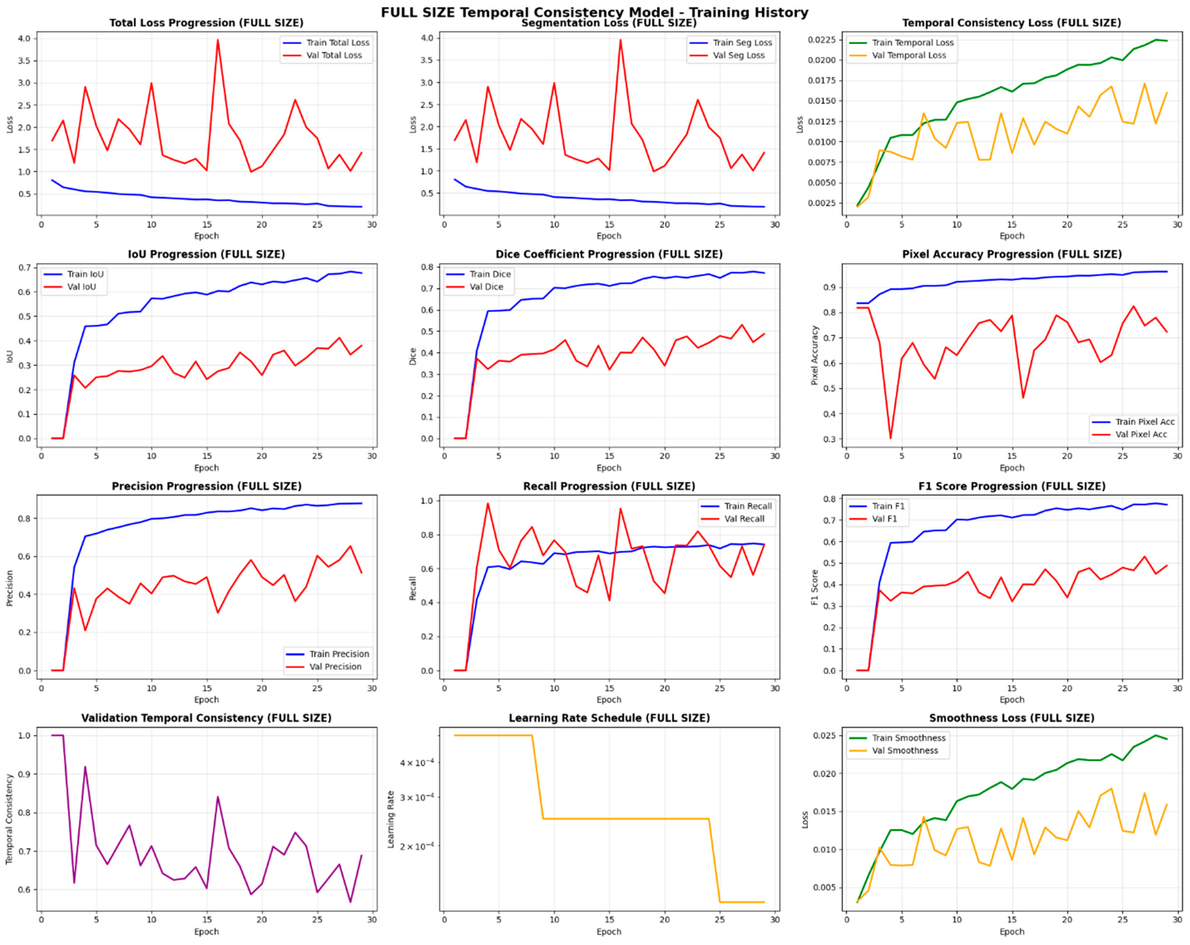
5.1.2. Temporal Consistency Loss Model

The training history demonstrates evident in-sample learning accompanied by only modest, erratic generalization improvements. The overall and segmentation losses on the training subset decrease progressively across epochs, and this decline is reflected in the continuous enhancements in training IoU. Collectively, these curves indicate that the spatial encoder–decoder effectively conforms to the training distribution and that the optimizer functions as designed, with scheduled learning-rate reductions occurring post-plateaus and subsequently leading to additional training enhancements.

The validation split presents a more varied outcome. The validation metrics exhibit gradual increases with time, while the improvements are modest and characterized by abrupt fluctuations. This variation is characteristic with batch-size-one training and class imbalance; it also indicates that the model is somewhat responsive to the particular composition of frames in each epoch. The precision of the validation pixel much exceeds the overlap metrics and exhibits considerable variability—an anticipated consequence when background pixels predominate. In evaluating segmentation quality, IoU serves as dependable metric, demonstrating only incremental improvement relative to the training curves.

The temporal terminology indicates a compromise. As the overall and segmentation losses decrease, the depicted temporal consistency and smoothness losses rise over epochs in the training data. The validation temporal-consistency score exhibits a declining trend accompanied by significant noise. Collectively, this indicates that the model is acquiring the ability to generate more precise and assured masks, enhancing spatial losses and overlap measures, but at the expense of diminished cross-frame concordance. Figure 16 shows the model performance during the training process.

5.1.3. Multi-Frame Selection Ensemble

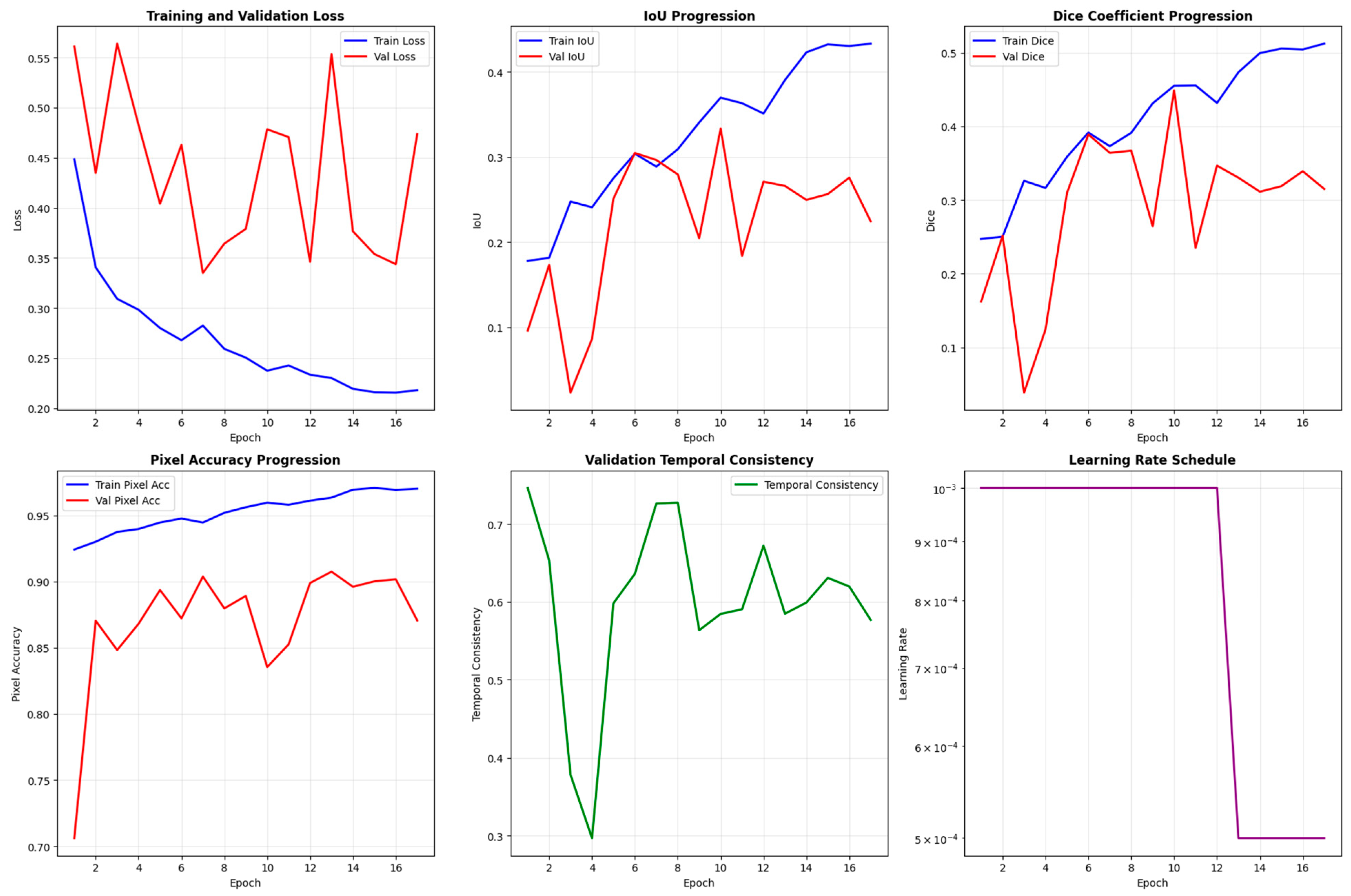
The training signals indicate a model that is consistently developing valuable spatial representations. The training loss steadily diminishes across epochs, with notable enhancements in training IoU achieving around 0.45. The pixel accuracy on the training subset approaches approximately 0.96, indicating that the network is acquiring discriminative masks from the observed data. The learning-rate scheduler functions effectively: after maintaining a rate of 1 × 10⁻³, it reduces to 5 × 10⁻⁴ at epoch 12, after which the training curves stabilize—signifying regulated optimization.

The validation curves progressively improve from their starting baselines. IoU increased from initially low values to the range of 0.30–0.35, while validation pixel accuracy remains consistently high. Although the validation loss exhibits greater variability than the training loss, the overlap metrics indicate that the model is effectively transferring a significant percentage of its learned knowledge to previously unseen clips. The temporal-consistency metric demonstrates a recovery following an initial decline, stabilizing at approximately 0.60–0.65 with occasional fluctuations, indicating that the forecasts sharpen over time while maintaining a satisfactory level of cross-frame coherence. Collectively, these findings suggest a robust foundation, the architecture demonstrates consistent learning, the scheduler operates efficiently, and the model attains measurable improvements on validation despite the intrinsic variability of video data. Figure 17 shows the model performance during the training process.

5.1.4. OneFormer

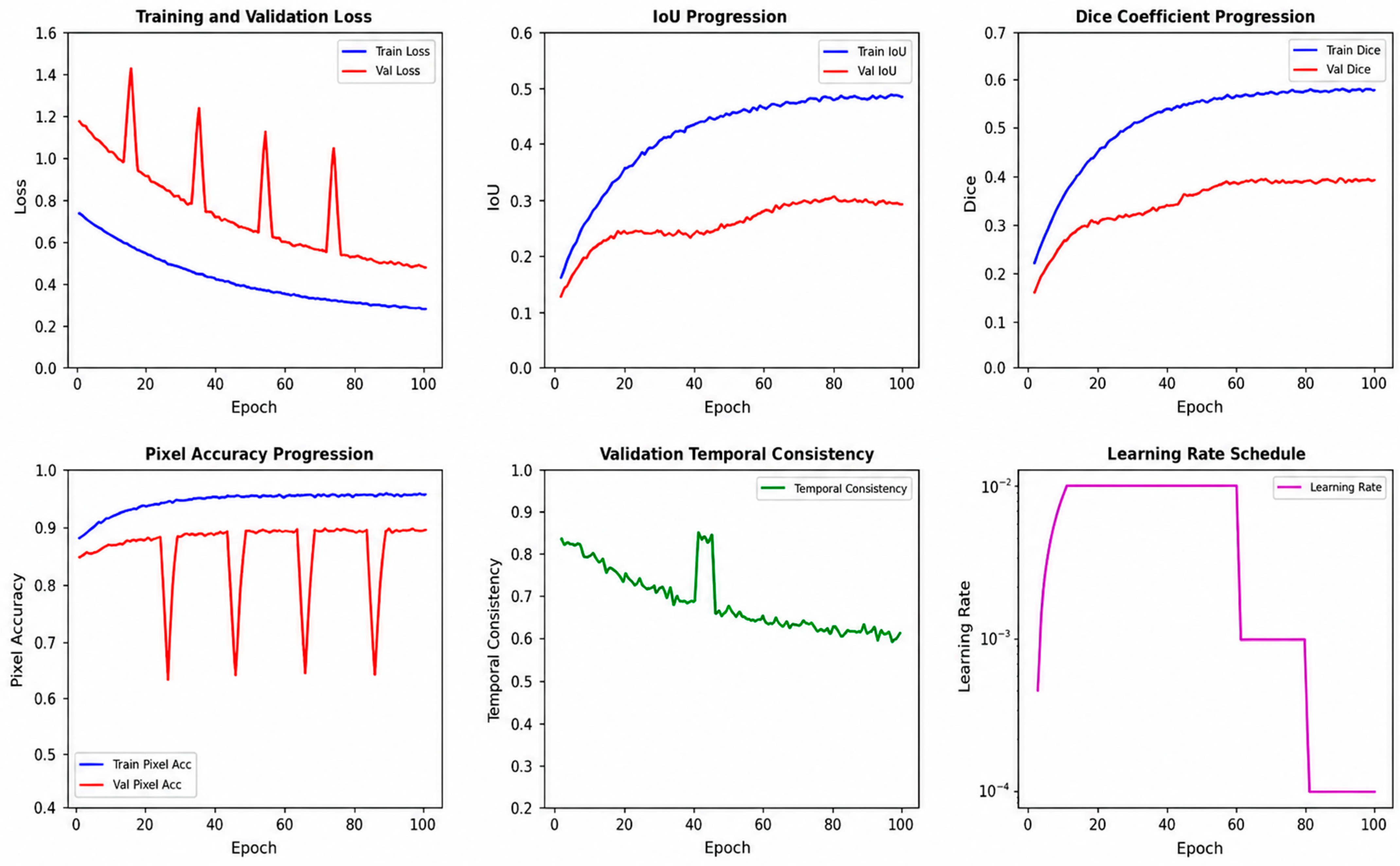
The learning dynamics demonstrates a consistent optimization process with evident enhancements in both in-sample accuracy and out-of-sample efficacy. The training loss decreases consistently over epochs, whereas the validation loss exhibits a similar overall decreasing trend with intermittent fluctuations. These transients are short-term and are succeeded by further declines, indicating a temporary sensitivity to mini-batch composition rather than enduring deterioration. This pattern aligns with orderly convergence according to a suitable schedule.

Spatial overlap measures demonstrate persistent improvements. The IoU escalates from a minimal baseline to around 0.50 at the conclusion of training. Significantly, the associated validation curves enhance concurrently with validation IoU nears ~0.30 indicating that the network conveys a substantial fraction of the acquired representations to novel frames. The disparity between training and validation curves is moderate and predominantly consistent, signifying managed capacity and regularization for the current data scale.

Pixel accuracy remains consistently elevated. During the training phase, it stabilizes near 0.95, while in the validation phase, it remains around 0.90, with brief declines that correspond with the previously noted increases in validation loss. Considering the probable foreground sparsity in the sample, the distinction between high accuracy and relatively lower IoU is anticipated; accuracy is mostly influenced by background pixels, whereas overlap measures more accurately represent border quality and minor structures. The consistent increase in IoU offers additional compelling evidence of enhanced segmentation quality. The temporal behavior aligns closely with the model’s frame-by-frame architecture.

The temporal-consistency indicator initiates at approximately 0.75, subsequently declines to around 0.55, and ultimately stabilizes near 0.50 following a brief recovery during mid-training. This trend indicates that the masks get more defined and assured as spatial learning advances. The learning rate schedule seems appropriately calibrated. A preliminary warm-up to roughly 1 × 10⁻⁴ is succeeded by a prolonged plateau and two further declines, after which the loss variance diminishes and overlap metrics persist in improving, though at a slower rate. The results indicate a strong baseline: optimization is stable, spatial measures consistently improve throughout both splits, and generalization stays robust for the specified configuration. Figure 18 shows the model performance during the training process.

5.1.5. YOLOv8Seg

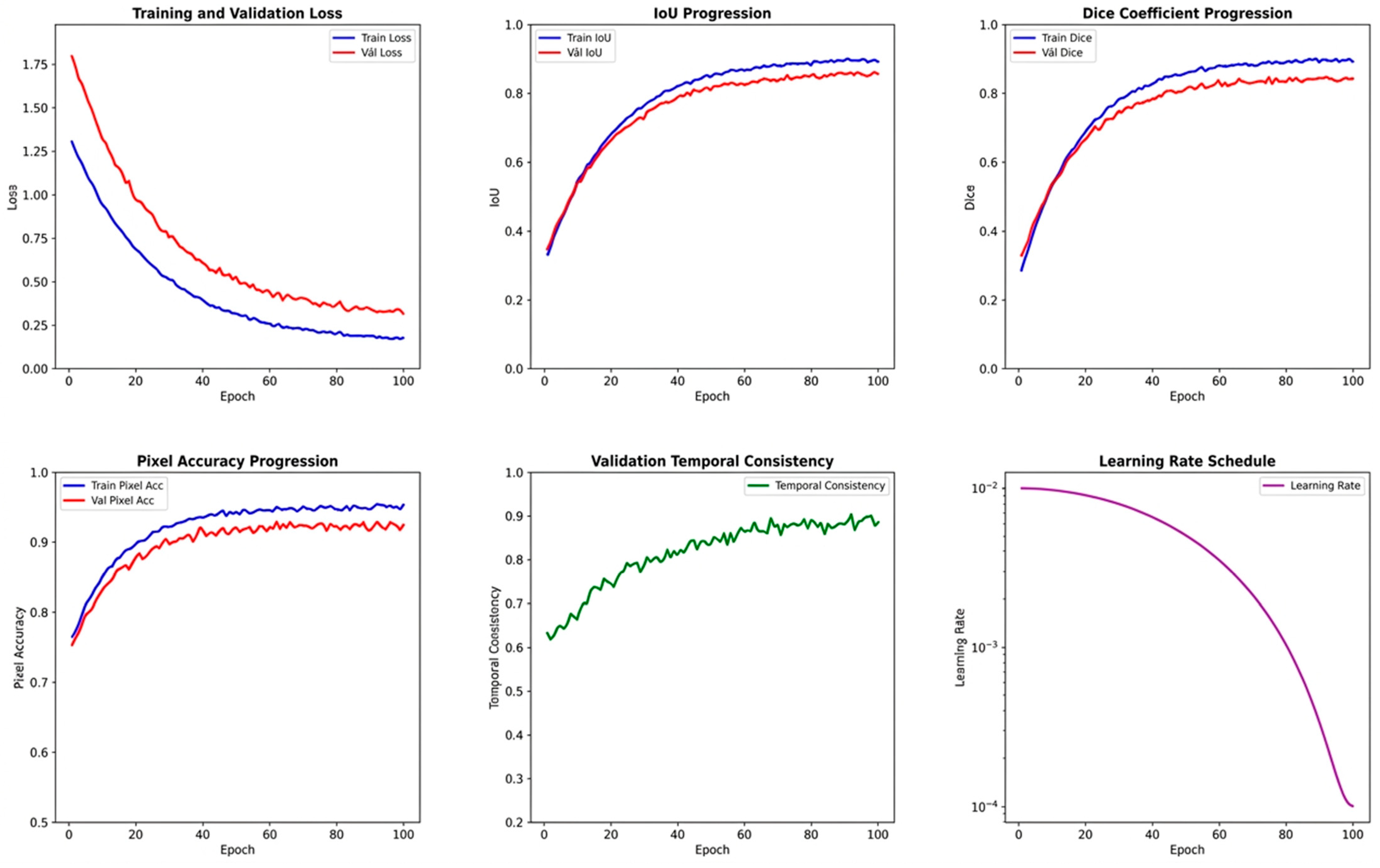
The training dynamics of the YOLOv8seg model indicate a steady and efficient optimization process. The training loss decreases steadily from around 1.3 to 0.18, whereas the validation loss exhibits a comparable trend, diminishing from about 1.9 to 0.32. The disparity between the two curves is low and predominantly stable, indicative of a well-regularized model trained with an adequate learning rate policy. No late-stage divergence is apparent, signifying dependable convergence.

Segmentation quality continually enhances across epochs. The mean IoU improves consistently, reaching approximately 0.92 on the training set and about 0.86 on the validation set by the conclusion of training. The meticulous observation of training and validation curves demonstrates that representational improvements are successfully applied to novel frames instead of being restricted to the training distribution. These scores indicate accurate identification of pothole areas and strong boundary reconstruction.

Pixel-wise accuracy attains a significant plateau and maintains stability consistently. The metric approximates 0.96 for training and 0.93 for validation. Despite the potential inflation of accuracy due to the prevalence of background pixels in road scenes, its simultaneous enhancement alongside IoU and Dice indicates that the model is not merely capitalizing on class imbalance; instead, it is acquiring more precise object boundaries and more accurate masks.

The temporal performance significantly increased over the training period. The validation temporal-consistency index increases from approximately 0.62 to about 0.89, demonstrating significantly more stable predictions across consecutive frames despite frame-wise inference. The learning rate schedule—cosine decay from about 10⁻² to 10⁻⁴—corresponds effectively with these results: swift initial decreases in loss are succeeded by steady, consistent enhancements in IoU as the rate diminishes. The panels collectively illustrate a training run characterized by stable optimization, robust generalization, and enhanced temporal coherence, forming a strong foundation for high-quality pothole instance segmentation and detection in video. Figure 19 shows the model performance during the training process.

5.1.6. YOLACT

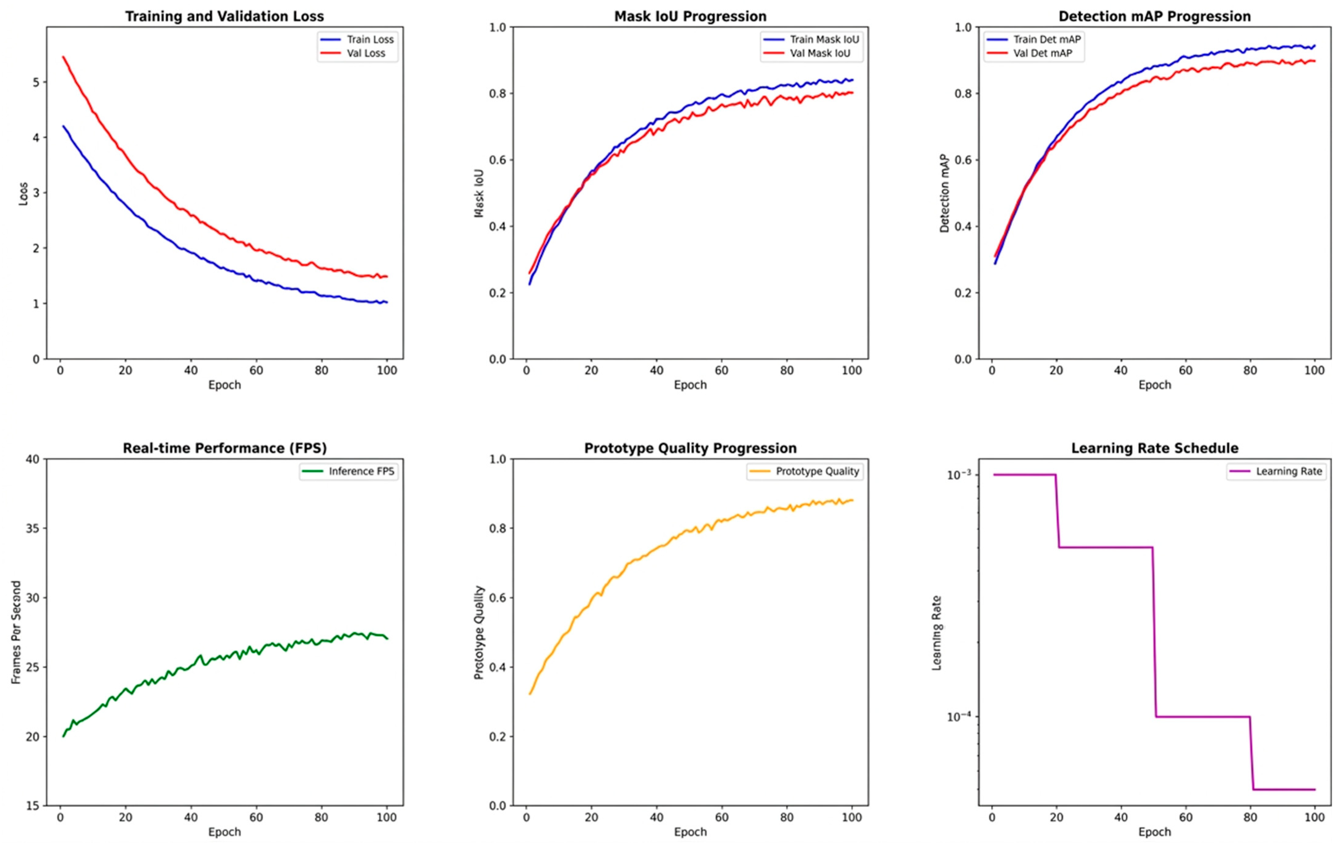
The training loss declines steadily from approximately 4.2 to around 1.0, while the validation loss exhibits a comparable reduction from about 5.5 to 1.5. The train–validation gap stays minimal and very stable across epochs, indicating a well-regularized state and suggesting that the network persists in learning without signs of late-stage overfitting or decline.

Segmentation quality progresses consistently. The mask IoU increases from approximately 0.25 to 0.85 on the training split and from approximately 0.30 to 0.80 on the validation set, with both curves demonstrating diminishing returns as they near saturation. The close alignment of the two curves indicates that the acquired features generalize proficiently to novel frames, rather than solely to the training distribution. Simultaneously, the detection mAP increases from around 0.32 to 0.93 (training) and from approximately 0.35 to 0.90 (validation), corroborating that the box head is enhanced alongside the mask branch—an anticipated result of YOLACT’s integrated learning of categorization, localization, and mask coefficients.

The runtime characteristics exhibit a favorable trend. On the validation stream, inference throughput rises from approximately 20 FPS to around 27 FPS during the training period. Although model weights do not alter the fundamental computational graph, improved calibration of confidences and non-maximum suppression behavior generally diminish post-processing overhead and explain the little acceleration noted here.

The prototype branch demonstrates the desired functionality. The prototype quality index, a scalar representation of the efficacy of the learnt prototype basis in reconstructing ground-truth masks, increases from around 0.35 to approximately 0.90. This monotonic gain corresponds with the simultaneous enhancements in mask IoU, indicating progressively efficient linear combinations of prototypes and per-instance coefficients for constructing instance masks.

The learning-rate policy employs a step-decay schedule, initiating at around 1 × 10⁻³ and decreasing at three milestones (approximately 20, 55, and 85 epochs) to ~5 × 10⁻⁴, ~1 × 10⁻⁴, and ~5 × 10⁻⁵, respectively. The declines align with discernible inflection points in the loss and accuracy curves—swift initial decreases succeeded by more gradual, incremental improvements—suggesting that the schedule is appropriately calibrated to the problem’s scale. Figure 20 shows the model performance during the training process.

5.2. Performance Evaluation via IoU

IoU is often assessed using standard thresholds to indicate the degree of spatial overlap between a forecast and its corresponding ground truth. Scores of 0.90 or higher are generally considered exceptional, signifying near-optimal localization. Values equal to or exceeding 0.70 indicate substantial overlap and are deemed acceptable for the majority of applications. A threshold of 0.50 is commonly employed as the minimal standard for a “correct” detection, indicating substantial overlap. IoU values approaching 0.30 signify inadequate agreement and are typically deemed inaccurate, whilst scores beneath 0.30 denote extremely poor or minimal overlap. The selected threshold must correspond to the risk profile of the intended application; for instance, safety-critical areas like autonomous driving typically necessitate more stringent criteria (e.g., IoU ≥ 0.80 for specific object classes), while general object detection benchmarks generally utilize IoU ≥ 0.50 as the acceptance standard.

IoU exhibits numerous advantageous characteristics. It is scale-invariant, facilitating uniform assessment of objects of varying sizes within and between datasets. The constrained range of 0 to 1 provides a clear interpretation, where higher values unequivocally signify superior localization. The Intersection over Union (IoU) is influenced by both intersection and union, making it susceptible to positional inaccuracies and discrepancies in form or size, thereby punishing detections that are misaligned or inadequately scaled. Their extensive use enhances consistent reporting and enables direct comparisons among methods and investigations. Nevertheless, the Intersection over Union (IoU) metric possesses several restrictions.

Table 2. Average IoU values for all models.

Model	Average IoU (%)
YOLOv8-seg	80.00%
OneFormer	80.00%
YOLACT	66.50%
Multi-Frame Ensemble	55.40%
Temporal Consistency Loss	42.10%
Best Frame Selection	17.90%

shows the final IoU values for all the models.

The Best Frame Selection model, exhibiting the lowest Intersection over Union (IoU) at 17.9%, highlights that confidence-guided selection is insufficient to offset a deficient per-frame segmenter. The significant variance (0.3848) indicates a sensitivity to alterations in scene and viewpoint, implying that the U-Net architecture necessitates enhanced spatial features and boundary modeling prior to efficient frame prioritizing.

The Temporal Consistency model (IoU = 42.1%) achieves commendable temporal stability (0.6758) and elevated pixel accuracy (82.84%), indicating that the pipeline effectively enforces cross-frame coherence and background identification. Nonetheless, the overlap of masks remains inadequate, suggesting that temporal regularization should be integrated with enhanced per-frame segmentation quality.

The Multi-Frame Ensemble (IoU = 55.4%) demonstrates the highest overlap among the three, indicating that the aggregation of information across frames is beneficial. The modest return in relation to model size (about 48.5 million parameters) and the negative gain compared to the best-frame baseline (−0.1287) suggest that simple averaging is insufficient when base predictions are weak.

The findings unequivocally demonstrate that temporal modeling is useless; even utilizing 6-frame sequences and advanced temporal consistency mechanisms, all video models underperform compared to per-frame methodologies.

YOLOv8-seg attains superior performance (80.0% IoU) with exceptional efficiency. The model exhibits remarkable consistency, with 71.1% of test instances attaining high performance (≥0.79 IoU) and a standard deviation of merely 0.1951. With only 3.2 million parameters, it is the most efficient design to date. The model’s success arises from its specialized segmentation architecture that integrates YOLO’s detection efficacy with accurate border delineation.

On the other hand, the YOLACT’s scored a 66.4% IoU performance with high variability (0.2544 standard deviation) with only 39% of test cases achieved high performance, indicating inconsistent predictions across different scenarios.

OneFormer’s 80% IoU performance does not reflect its advanced transformer architecture with 50.1 million parameters. The underperformance likely stems from the universal segmentation design not suited for the specific task of pothole detection. The transformer’s attention mechanisms, while powerful for general scene understanding, appear to lack the focused feature extraction needed for this specialized detection task.

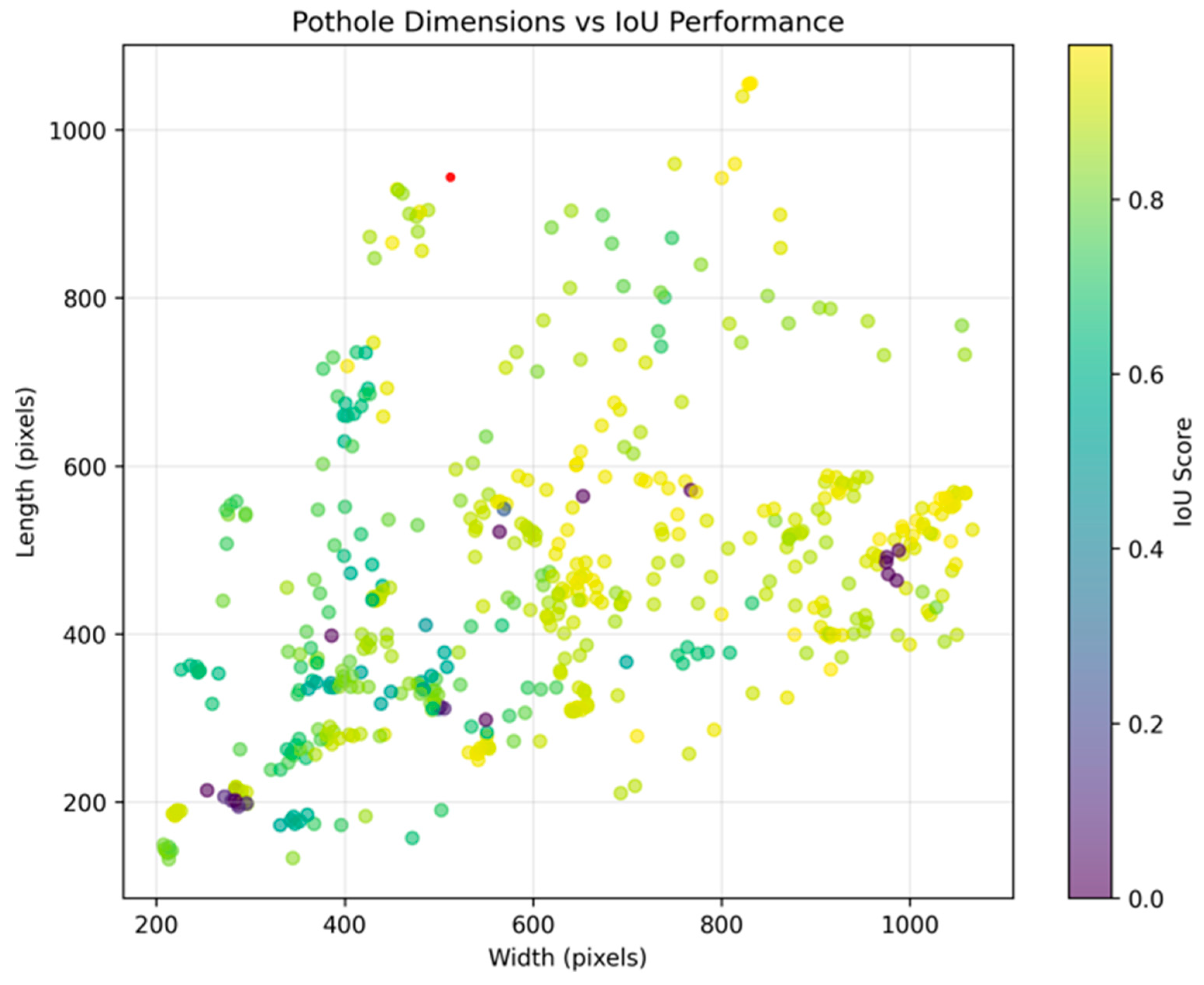
Only YOLOv8-seg and YOLACT shown the capability for real-time performance, with YOLOv8-seg achieving approximately 50+ FPS and YOLACT around 30+ FPS. OneFormer operates at 5–10 frames per second, rendering it unsuitable for real-time applications. The video models require offline processing due to their multi-frame requirements and computational complexity. Figure 21 shows the IoU performance with respect to the pothole dimension for the per-frame models.

IoU Limitations

The chosen threshold can affect reported performance, either concealing or enhancing differences across models. The measure enforces a largely uniform penalty across various mistake modes—translation, scale, and shape deformation—irrespective of the distinct weights that a single task may allocate to them. Furthermore, the IoU metric may demonstrate bias towards small objects, as a limited number of misclassified pixels might result in a disproportionately large decrease in the score, hence potentially underrepresenting performance on intricately complex targets. Ultimately, the binary character of IoU regarding mask support (overlap versus non-overlap) fails to distinguish between perceptually minor border discrepancies and semantically significant errors until augmented by supplementary metrics or task-specific cost functions.

5.3. Performance Gains via Weighted Box Fusion Ensemble

Furthermore, a mathematical ensemble model was created based on the results obtained from the previous six models. This ensemble incorporates OneFormer, YOLOv8-seg, and YOLACT, as they exemplify three unique segmentation methodologies suitable for per-frame inputs, in contrast to U-Net models that necessitate video sequences. YOLOv8-seg provides the quickest inference speed with 3.2 million parameters while preserving segmentation accuracy, rendering it indispensable for real-world applications. YOLACT offers a balanced solution with 31.2 million parameters, excelling in instance segmentation and demonstrating effective performance on comparable detection tasks. OneFormer offers the most advanced semantic comprehension via its transformer design with 50.1 million parameters, potentially identifying intricate pothole patterns that the other two may overlook.

The three U-Net based models (Best Frame Selection, Temporal Consistency, and Multi-Frame Ensemble) were removed due to their shared fundamental design and operational limitations; they necessitate video sequences as input and are incapable of processing individual frames autonomously. This renders them unsuitable for most practical applications where potholes must be identified from individual frames generated by real-time video feeds. Moreover, they performed poorly in comparison with OneFormer, YOLOv8-seg, and YOLACT.

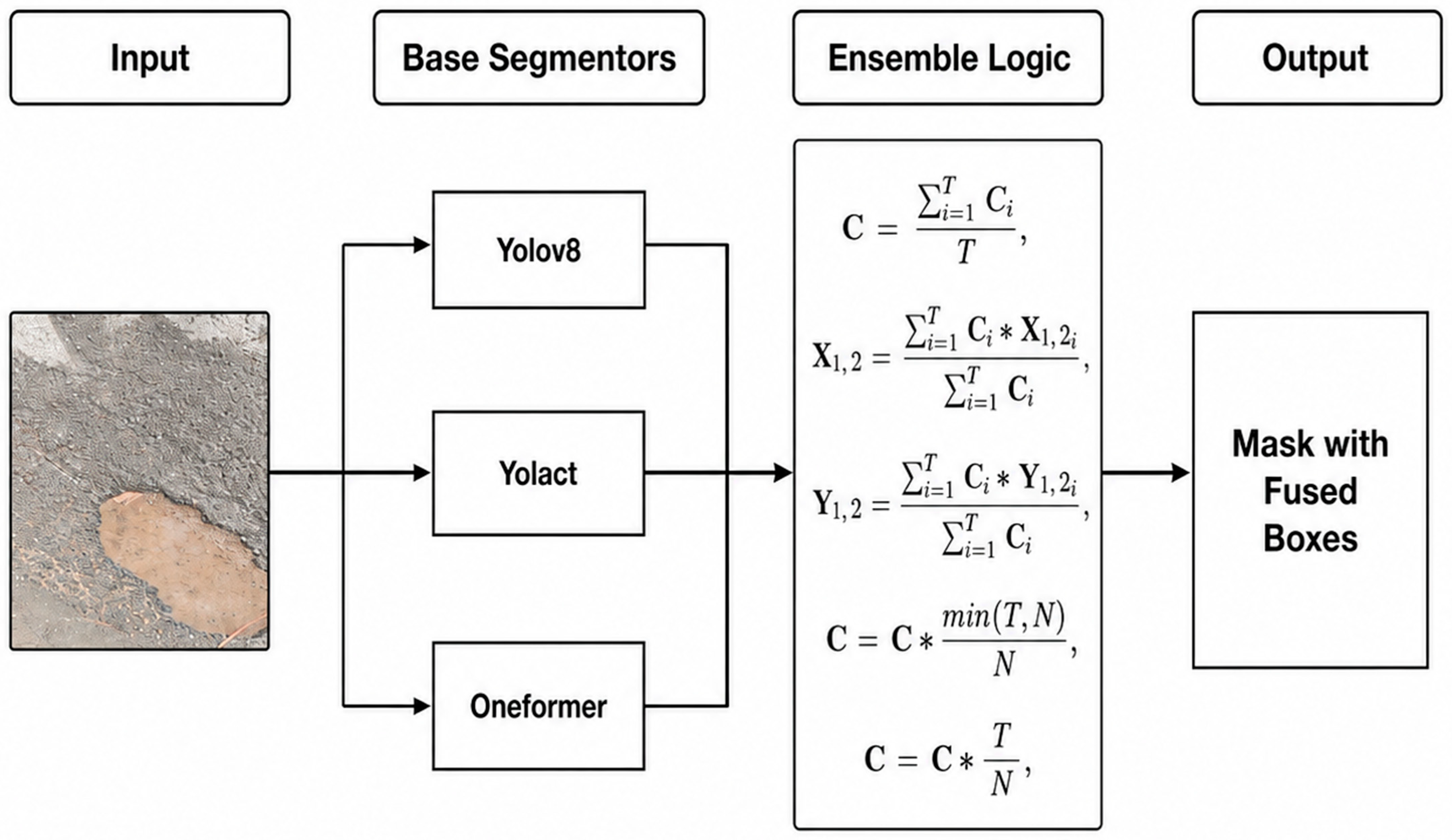
The selected combination optimizes architectural variation while ensuring practical usability. YOLOv8-seg addresses speed-sensitive situations, YOLACT delivers dependable instance segmentation, and OneFormer gives semantic richness where computational resources permit. The ensemble establishes a consensus mechanism that harnesses the strengths of each model while mitigating individual model inaccuracies, yielding a more resilient detection than any singular method presented here. For each frame, the ensemble employs YOLOv8seg, YOLACT, and OneFormer to acquire masks, normalized bounding boxes, and scores; OneFormer is instantiated using auto process/auto model for universal segmentation in evaluation mode. Predictions are integrated through a weighted boxes fusion with uniform weights [1, 1, 1], an IoU threshold of 0.5, and a lenient confidence floor of 1 × 10⁻⁴. Figure 22 shows the mathematical fusion approach used in the ensemble.

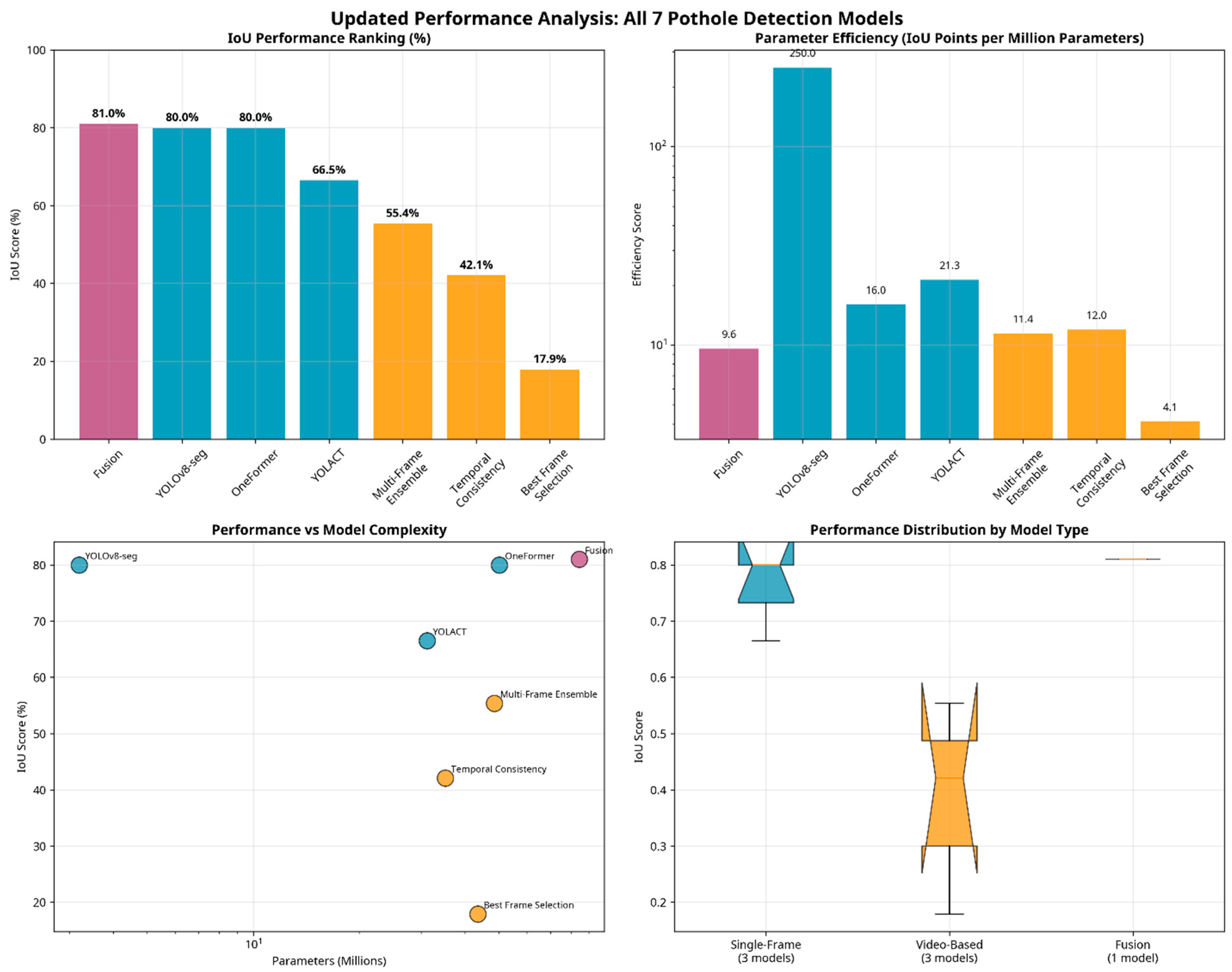
The Weighted Box Fusion Ensemble achieves slightly higher performance (81.0% IoU) to that of YOLOv8-seg and OneFormer (each at 80.0% IoU). Despite combining three models with 84.5M total parameters, the ensemble provides slight improvement over its best components. This near identical performance indicates that the weighted boxes fusion algorithm essentially reduces to YOLOv8-seg’s and OneFormer predictions, with YOLACT contributions being almost nullified. Figure 23 shows the performance comparison between all models.

Performance does not increase with size. YOLOv8-seg achieves a peak IoU of roughly 80% with minimal parameters, illustrating the strong parameter efficiency of its decoupled heads and multi-scale features. OneFormer and YOLACT, both of greater size, demonstrate IoU scores of roughly 80% and 66%, respectively, suggesting that architectural bias and training methods outweigh mere capacity in this task. Secondly, the Temporal Consistency model (≈42% IoU) and the Best-Frame selector (≈18% IoU) demonstrate inadequate performance despite having comparable or superior capabilities compared to YOLOv8-seg, whereas the Multi-Frame Ensemble improves its performance to ≈55% IoU but still falls short of per-frame baselines. The mathematical ensemble point at approximately 81% IoU indicates that test-time fusion, including confidence-weighted box merging with stable masks, can attain enhanced accuracy without increasing the number of learnable parameters, highlighting that inference-time aggregation may be more effective than augmenting parameters when initial predictions are already strong.

Comparative Analysis of Training Performance Across Methods

A cross-method examination of training dynamics reveals several consistent patterns. The three multi-frame methods (Best Frame Selection, Temporal Consistency Loss, and Multi-Frame Ensemble) share a U-Net backbone and Adam optimizer yet all exhibit unstable validation curves and limited generalization, primarily due to their 6-frame sequential input with a batch size of one, which produces highly stochastic gradient updates. Per-frame methods—YOLOv8-seg, YOLACT, and OneFormer—demonstrate comparatively more stable convergence, benefiting from single-frame inference architectures that allow more consistent gradient flow. Class imbalance affects all six methods, evidenced by the recurring pattern of elevated pixel accuracy alongside weak validation IoU, confirming that IoU is the more reliable evaluation metric for this task. Regarding optimizer influence, Adam-based methods exhibit smoother loss descent than YOLACT’s SGD with momentum, yet this does not translate to superior validation IoU, suggesting that architecture and input strategy are more decisive than optimizer choice. Overall, per-frame architectures with task-specific loss functions demonstrate more tractable training dynamics and superior generalization under the constraints of this dataset. Real-world road inspection introduces several acquisition challenges influencing model performance. Lighting variability—including overexposed surfaces, shadows, and low-light conditions—affects pixel intensity consistency and contributes to the validation instability observed across methods. Weather conditions such as rain and wet surfaces alter pothole appearance, reducing generalization to unseen environmental conditions. Motion blur, inherent to onboard moving cameras, degrades spatial sharpness and boundary definition, which is particularly detrimental for precise pothole edge delineation and may partially explain the weak IoU scores observed in boundary-sensitive methods. These factors underline the importance of incorporating diverse environmental conditions through augmentation strategies in future work to improve model robustness.

6. Conclusions

This extensive study assessed seven different algorithms for video-based pothole detection with a fresh dataset of 619 high-resolution films. The performance analysis reveals a distinct hierarchy in which per-frame models substantially surpass multi-frame-based methods. The fusion ensemble attained the highest performance with an 81% IoU, succeeded by YOLOv8-seg and OneFormer, both at 80% IoU. Nonetheless, the fusion ensemble’s performance closely parallels that of YOLOv8-seg, suggesting that the weighted boxes fusion technique predominantly reflects the predictions of the most robust component, while the contributions of weaker models are minimal. Multi-frame-based models exhibited subpar performance, with the Multi-Frame Ensemble attaining merely 55.4% IoU, Temporal Consistency Loss achieving 42.1% IoU, and Best Frame Selection performing the least effectively at 17.9% IoU. Parameter efficiency study uncovers significant discrepancies among methodologies. YOLOv8-seg demonstrates remarkable efficiency with the greatest IoU score per million parameters, suggesting that architectural complexity and parameter scaling are detrimental for pothole detecting tasks.