Economical, Optimal and Uncertain Multiple-View L₂ Triangulation via LMIs

Abstract

This paper proposes a novel approach for multiple-view $L_2$ triangulation, a key problem in computer vision which consists of estimating a scene point from its estimated image projections on two or more cameras and from the estimated projection matrices of the cameras by minimizing the reprojection error in the $L_2$ norm. In the proposed approach, the estimated image projections are allowed to be uncertain in admissible regions described by polynomial inequalities and equalities, and an estimate of the scene point is obtained by solving a linear matrix inequality (LMI) problem built with matrix decompositions, polynomial multipliers, and the Gram matrix method. It is proven that the optimal estimate can always be achieved by using multipliers with sufficiently large degree. Moreover, a simple test is provided in order to establish the optimality of the obtained estimate. As shown by some examples with real and synthetic data, the proposed approach presents key advantages with respect to several existing methods of a different nature, which may fail to find the optimal estimate, may not allow one to establish the optimality of the found estimate, or may require a larger computational burden.

1. Introduction

Multiple-view triangulation is the problem of estimating a scene point from its estimated image projections on two or more cameras and from their estimated projection matrices; see, e.g., [1,2]. This problem is important in various applications, such as map building, object reconstruction, visual servoing, etc.

A simple method for addressing multiple-view triangulation consists of minimizing the algebraic error in the estimated projective relationship between the candidate scene point and its estimated image projections. This method only requires the solution of a linear least-squares optimization, but the obtained estimates can be unsatisfactory. In order to provide more accurate estimates, other methods have been proposed in the literature, generally aimed at minimizing a geometrical error defined as the estimated reprojection error, i.e., the mean of the distances between the image projections of the candidate scene point provided by the estimated projection matrices and its estimated image projections. These distances are typically defined via the $L_2$ norm (i.e., defined as Euclidean distances) due to its isomorphic property; see, e.g., refs. [3,4,5] about multiple-view triangulation with the reprojection error defined via other norms.

Multiple-view $L_2$ triangulation is a nontrivial problem as it is equivalent to a rational least-squares optimization where the function to be minimized can be nonconvex. Various methods have been proposed in the literature for addressing this problem, which include the pioneering methods [1,6] based on the solution of system of polynomial equations for the cases of two and three views, the method [7] based on the recursive partition of the search space via branch-and-bound algorithms, the method [8] based on the use of evolutionary computational techniques, and the method [9] based on reducing the complexity of geometric vision problems through the targeted reweighting of the cost functions used to minimize reprojection errors.

In spite of these contributions, multiple-view $L_2$ triangulation remains a challenging problem in practice. One reason is that the sought scene point may be uncertain in some views due to possible occlusions caused by objects, with the consequence that admissible regions (rather than just points) should be allowed for the estimated image projections. For instance, such admissible regions could be one-dimensional sets such as lines and curves, or two-dimensional sets such as rectangles, polytopes and ellipses. Clearly, this increases the difficulty of the resulting multiple-view $L_2$ triangulation (which is referred to as uncertain multiple-view $L_2$ triangulation in this paper), since the cost function to be minimized may be irrational and may not have an explicit expression.

A possibility for addressing uncertain multiple-view $L_2$ triangulation consists of exploiting numerical methods for nonlinear optimization. However, given the fact that the function to be minimized can be nonconvex, these methods have two main weaknesses. The first weakness is that the solution provided by these methods can depend on the chosen initialization, and it is unclear how such an initialization should be chosen in order to guarantee that the found solution is a global minimizer. The second weakness is that these methods do not allow one to establish if the found solution is a global minimizer. In other words, these methods do not guarantee the achievement or recognition of optimal estimates sought in the uncertain multiple-view $L_2$ triangulation; see, e.g., refs. [10,11,12] for a comprehensive collection of numerical methods for nonlinear optimization and for detailed discussions about the limitations previously mentioned when used for solving nonconvex optimization problems. In order to cope with these issues, two methods known as TFML and TPML have been proposed in [13] for uncertain multiple-view $L_2$ triangulation based on the solution of LMI problems built with the use of sums of squares of polynomials (SOS). However, the estimates provided by these two methods may be not optimal, and the computational burden can be prohibitive; see, e.g., ref. [14] for the complexity of SOS programming.

Before proceeding, it is worth mentioning that camera pose estimation and camera calibration are problems closely related to multiple-view triangulation. Indeed, camera pose estimation consists of estimating the relative orientation and translation among two or more cameras from the estimated image projections of a set of scene points and possibly additional information about the position of such points. Also, camera calibration consists of estimating the intrinsic camera parameters, such as the focal lengths, aspect ratio, and camera center. The relative orientation and translation among the cameras, together with the intrinsic camera parameters, determine the projection matrices used to define multiple-view triangulation, which is used for a number of tasks such as scene reconstruction and human pose estimation. Recent works in these areas include various contributions. For instance, camera pose estimation is addressed in [15] via integration with machine learning model, in [16] via weighted M-estimate sample consensus, and in [17] based on the analytical elimination of translation. Human pose estimation is studied in [18] using appearance similarity and in [19] via the combination of multiple views and wearable inertia measurement units. Scene reconstruction is considered in [20] for the case of complex objects and in [21] using ray regression and deep learning. Also, camera calibration is addressed in [22] by using full camera models, in [23] for heterogeneous cameras, in [24] for portable monocular cameras, in [25] using a starling-inspired strategy optimization algorithm, and in [26] through online cascade optimization.

This paper proposes a novel approach for uncertain multiple-view $L_2$ triangulation where the estimated image projections are allowed to be uncertain in admissible regions described by polynomial inequalities and equalities. Firstly, this problem is transformed by introducing variables in the image domain rather than in the 3D space. Secondly, the semialgebraic set constraining these variables is re-elaborated by using a singular-value decomposition (SVD) in order to obtain a minimal description of the required polynomials. Thirdly, candidate image variables corresponding to the optimal estimate of the scene point are obtained by solving an LMI problem, in particular, a generalized eigenvalue problem (GEVP) or a semidefinite program (SDP), built with the introduction of polynomial multipliers and the use of the Gram matrix method. Lastly, an estimate of the scene point is recovered as the scene point matching such candidates through linear algebra operations on matrices obtained from the solution of the LMI problem. It is proven that the optimal estimate can always be achieved by using multipliers with sufficiently large degree. Moreover, a simple test is provided in order to establish the optimality of the obtained estimate. As shown by some examples with real and synthetic data, the proposed approach presents key advantages with respect to several existing methods of a different nature. Specifically, these examples show that the existing methods based on nonconvex optimization may fail to find the optimal estimate or may not allow one to establish their optimality of the found estimate, while the existing methods based on convex optimization may fail to find the optimal estimate or may require a larger computational burden.

The paper is organized as follows. Section 2 introduces the preliminaries. Section 3 states the problem formulation. Section 4 describes the proposed approach. Section 5 presents the examples. Lastly, Section 6 reports the conclusions.

2. Preliminaries

Let us start by introducing the notation adopted throughout the paper:

• $\mathbb{N},\mathbb{R}$: sets of nonnegative integers and real numbers.
• ${\mathbf{I}}_n$: $n\times n$ identity matrix.
• ${\mathbf{0}}_n$: $n\times 1$ null vector (empty vector $0\times 1$ for $n=0$).
• ${\mathbf{A}}^T$: transpose of matrix $\mathbf{A}$.
• ${\mathbf{A}}^{†}$: pseudo-inverse of matrix $\mathbf{A}$.
• ${\parallel \mathbf{A}\parallel }_2$,${\parallel \mathbf{A}\parallel }_{\infty }$: 2-norm and infinity-norm of matrix $\mathbf{A}$.
• $\mathbf{A}>0$ (resp., $\mathbf{A}\ge 0$): entrywise positive (resp., nonnegative) matrix $\mathbf{A}$.
• $\mathbf{A}\succ 0$ (resp., $\mathbf{A}⪰0$): positive definite (resp., semidefinite) matrix $\mathbf{A}$.
• $diag\left(\mathbf{a}\right)$: diagonal matrix with the $(i,i)$-th entry equal to the i-th entry of vector $\mathbf{a}$.
• ${\left[\mathbf{a}\right]}_{\times }$: skew-symmetric matrix defined by vector $\mathbf{a}$.
• $SO\left(3\right)$: $\{\mathbf{R}\in {\mathbb{R}}^{3\times 3}:{\mathbf{R}}^T\mathbf{R}=\mathbf{R}{\mathbf{R}}^T={\mathbf{I}}_3\}$.
• $SE\left(3\right)$: $SO\left(3\right)\times {\mathbb{R}}^3$.
• $deg\left(\mathbf{A}\right(\mathbf{v}\left)\right)$: degree of matrix polynomial $\mathbf{A}\left(\mathbf{v}\right)$.

Let $\mathbf{X}\in {\mathbb{R}}^3$ be a scene point observed by a perspective camera with coordinate frame $F=(\mathbf{R},\mathbf{t})\in SE\left(3\right)$. Let $\mathbf{x}\in {\mathbb{R}}^2$ be the image projection of $\mathbf{X}$ onto the camera. The relation between $\mathbf{X}$ and $\mathbf{x}$ is given by

$$\beta \left(\begin{array}{c}\mathbf{x}\\ 1\end{array}\right)=\mathbf{P}\left(\begin{array}{c}\mathbf{X}\\ 1\end{array}\right)$$

(1)

where $\beta \in \mathbb{R}$ is a scaling factor and $\mathbf{P}\in {\mathbb{R}}^{3\times 4}$ is the projection matrix of the camera given by

$$\mathbf{P}=\mathbf{K}\left(\mathbf{R},\mathbf{t}\right)$$

(2)

where $\mathbf{K}\in {\mathbb{R}}^{3\times 3}$ is the upper triangular matrix containing the intrinsic parameters of the camera. It follows that

$$\beta =\left(\begin{array}{ccccc}0& ,& 0& ,& 1\end{array}\right)\mathbf{P}\left(\begin{array}{c}\mathbf{X}\\ 1\end{array}\right),$$

(3)

and, hence, the function providing $\mathbf{x}$ from $\mathbf{P}$ and $\mathbf{X}$ in (1) is given by

$$\mathbf{\Phi }(\mathbf{X},\mathbf{P})={\displaystyle \frac{\left(\begin{array}{ccccc}1& ,& 0& ,& 0\\ 0& ,& 1& ,& 0\end{array}\right)\mathbf{P}\left(\begin{array}{c}\mathbf{X}\\ 1\end{array}\right)}{\left(\begin{array}{ccccc}0& ,& 0& ,& 1\end{array}\right)\mathbf{P}\left(\begin{array}{c}\mathbf{X}\\ 1\end{array}\right)}}.$$

(4)

3. Problem Formulation

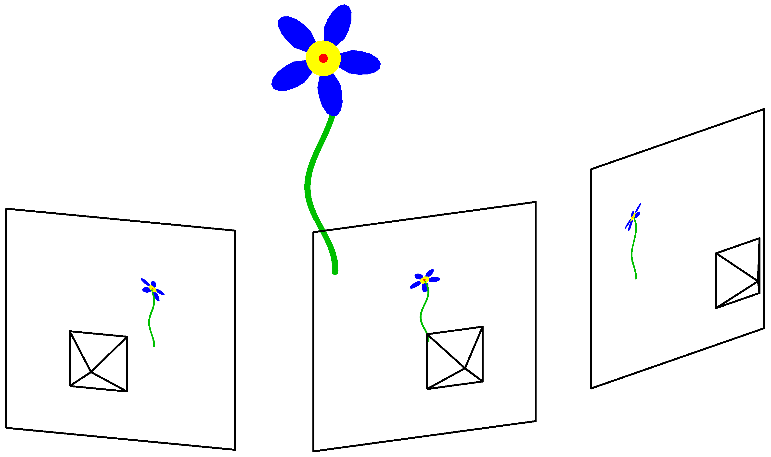
Multiple-view triangulation consists of estimating the scene point from the knowledge of its image projections in two or more cameras and from the knowledge of the projection matrices of such cameras—see Figure 1 for an illustration. In the ideal case where the image projections and the projection matrices are known, the scene point can be recovered by exploiting (1), which consists of solving a system of linear equations. However, in the real case, the image projections and the projection matrices are unknown due to image noise and calibration errors, and the problem consists of estimating the scene point from their available estimates by minimizing an error, typically chosen as the mean square re-projection error in the $L_2$ norm. Moreover, the available estimate of each image projection may be not just a single point but, due to possible occlusions, an admissible region.

Hence, in this paper, we address an uncertain multiple-view $L_2$ triangulation problem, which is formulated as follows. Consider a scene point ${\mathbf{X}}_{obj}\in {\mathbb{R}}^3$ observed by N cameras. The problem consists of estimating ${\mathbf{X}}_{obj}$ from the estimates ${\widehat{\mathbf{P}}}_i$ of the projection matrices of these cameras and from the admissible regions ${\widehat{\mathcal{R}}}_i\subset {\mathbb{R}}^2$ for the image projections ${\mathbf{o}}_i$ of ${\mathbf{X}}_{obj}$ on these cameras, $i=1,\dots ,N$, by minimizing the mean square re-projection error in the $L_2$ norm. It is assumed that the admissible regions ${\widehat{\mathcal{R}}}_i$ can be described by polynomial inequalities and equalities in the image space.

Specifically, let $\mathbf{X}\in {\mathbb{R}}^3$ be the variable scene point used to search for the estimate of ${\mathbf{X}}_{obj}$. The uncertain multiple-view $L_2$ triangulation problem considered in this paper is

$${\gamma }^{*}=\underset{\mathbf{X}\in {\mathbb{R}}^3}{inf}\gamma \left(\mathbf{X}\right)$$

(5)

where $\gamma \left(\mathbf{X}\right)$ is defined as

$$\gamma \left(\mathbf{X}\right)=\sqrt{{\displaystyle \frac{1}{2N}}\sum _{i=1}^{N}d{(\mathbf{\Phi }(\mathbf{X},{\widehat{\mathbf{P}}}_i),{\widehat{\mathcal{R}}}_i)}^2}$$

(6)

and $d(\mathbf{\Phi }(\mathbf{X},{\widehat{\mathbf{P}}}_i),{\widehat{\mathcal{R}}}_i)$ is the Euclidean distance from the image projection $\mathbf{\Phi }(\mathbf{X},{\widehat{\mathbf{P}}}_i)$ to the admissible region ${\widehat{\mathcal{R}}}_i$, i.e.,

$$d(\mathbf{\Phi }(\mathbf{X},{\widehat{\mathbf{P}}}_i),{\widehat{\mathcal{R}}}_i)=\underset{\mathbf{x}\in {\widehat{\mathcal{R}}}_i}{inf}{∥\mathbf{\Phi }(\mathbf{X},{\widehat{\mathbf{P}}}_i)-\mathbf{x}∥}_2.$$

(7)

The estimate ${\mathbf{X}}^{*}$ of the scene point ${\mathbf{X}}_{obj}$ provided by the uncertain multiple-view $L_2$ triangulation problem in (5) is defined as any minimizer of $\gamma \left(\mathbf{X}\right)$, i.e.,

$${\mathbf{X}}^{*}\in arg\underset{\mathbf{X}\in {\mathbb{R}}^3}{inf}\gamma \left(\mathbf{X}\right).$$

(8)

4. Proposed Approach

This section describes the proposed approach. Specifically, Section 4.1 introduces a reformulation of problem via polynomials, Section 4.2 illustrates typical admissible regions for the image projections, Section 4.3 explains how to consider projection constraints, Section 4.4 reviews the Gram matrix method, Section 4.5 introduces the optimization problem, Section 4.6 explains how the estimate is constructed, Section 4.7 presents the main result, and Section 4.8 describes a simplified case.

4.1. Part I: Reformulation via Polynomials

Let us start by defining the estimated image projection of the variable scene point $\mathbf{X}\in {\mathbb{R}}^3$ onto the i-th camera as

$${\mathbf{x}}_i=\mathbf{\Phi }(\mathbf{X},{\widehat{\mathbf{P}}}_i).$$

(9)

The first step of the proposed approach consists of introducing auxiliary variables ${\mathbf{y}}_i\in {\mathbb{R}}^{n_i}$, $i=1,\dots ,N$, (where $n_i=0$ if ${\mathbf{y}}_i$ is not needed) in order to express the following:

• The condition that ${\mathbf{x}}_i$ belongs to the region ${\widehat{\mathcal{R}}}_i$ in terms of polynomial equalities and inequalities in ${\mathbf{x}}_i$ and ${\mathbf{y}}_i$;
• The squared Euclidean distance from ${\mathbf{x}}_i$ to the region ${\widehat{\mathcal{R}}}_i$ as a quadratic function in ${\mathbf{x}}_i$ and ${\mathbf{y}}_i$.

• This process is clarified in Section 4.2 for some typical admissible regions ${\widehat{\mathcal{R}}}_i$ by using the following notation. Define the vector $\mathbf{v}\in {\mathbb{R}}^{N_v}$ as

$$\mathbf{v}={\left({\mathbf{x}}_1^T,\dots ,{\mathbf{x}}_N^T,{\mathbf{y}}_1^T,\dots ,{\mathbf{y}}_N^T\right)}^T$$

(10)

where

$$N_v=2N+n_1+\dots +n_N.$$

(11)

We express the condition

$${\mathbf{x}}_i\in {\widehat{\mathcal{R}}}_i$$

(12)

as

$$\left\{\begin{array}{ccc}\hfill {\mathbf{g}}_i\left(\mathbf{v}\right)& =& 0\hfill \\ \hfill {\mathbf{h}}_i\left(\mathbf{v}\right)& \ge & 0\hfill \end{array}\right.$$

(13)

for some vector polynomials ${\mathbf{g}}_i\left(\mathbf{v}\right)$ and ${\mathbf{h}}_i\left(\mathbf{v}\right)$ (which may be defined as the empty vector ${\mathbf{0}}_0$ if not needed). Moreover, we express the squared Euclidean distance from ${\mathbf{x}}_i$ to the admissible region ${\widehat{\mathcal{R}}}_i$ as

$$d{({\mathbf{x}}_i,{\widehat{\mathcal{R}}}_i)}^2=f_i\left(v\right)$$

(14)

for some quadratic functions $f_i\left(\mathbf{v}\right)$.

4.2. Part II: Typical Admissible Regions

Some cases of interest for the admissible regions ${\widehat{\mathcal{R}}}_i$ and the corresponding expressions (13) and (14) are as follows:

• Case I: ${\widehat{\mathcal{R}}}_i$ is a point, i.e.,

  $${\widehat{\mathcal{R}}}_i={\widehat{\mathbf{x}}}_i$$

  (15)

  for some ${\widehat{\mathbf{x}}}_i\in {\mathbb{R}}^2$. In this case, (13) and (14) hold with

  $$\left\{\begin{array}{ccc}\hfill n_i& =& 0\hfill \\ \hfill f_i\left(\mathbf{v}\right)& =& \parallel {\mathbf{x}}_i-{\widehat{\mathbf{x}}}_i{\parallel }_2^2\hfill \\ \hfill {\mathbf{g}}_i\left(\mathbf{v}\right)& =& {\mathbf{0}}_0\hfill \\ \hfill {\mathbf{h}}_i\left(\mathbf{v}\right)& =& {\mathbf{0}}_0;\hfill \end{array}\right.$$

  (16)
• Case II: ${\widehat{\mathcal{R}}}_i$ is a line segment, i.e.,

  $${\widehat{\mathcal{R}}}_i=\left\{{\widehat{\mathbf{x}}}_i+{\mathbf{y}}_i{\widehat{\mathbf{d}}}_i:{\mathbf{y}}_i\in [-1,1]\right\}$$

  (17)

  for some ${\widehat{\mathbf{x}}}_i,{\widehat{\mathbf{d}}}_i\in {\mathbb{R}}^2$. In this case, (13) and (14) hold with

  $$\left\{\begin{array}{ccc}\hfill n_i& =& 1\hfill \\ \hfill f_i\left(\mathbf{v}\right)& =& \parallel {\mathbf{x}}_i-{\widehat{\mathbf{x}}}_i-{\mathbf{y}}_i{\widehat{\mathbf{d}}}_i{\parallel }_2^2\hfill \\ \hfill {\mathbf{g}}_i\left(\mathbf{v}\right)& =& {\mathbf{0}}_0\hfill \\ \hfill {\mathbf{h}}_i\left(\mathbf{v}\right)& =& 1-{\mathbf{y}}_i^2;\hfill \end{array}\right.$$

  (18)
• Case III: ${\widehat{\mathcal{R}}}_i$ is a convex polytope, i.e.,

  $${\widehat{\mathcal{R}}}_i=\left\{{\mathbf{y}}_i\in {\mathbb{R}}^2:{\parallel {\widehat{\mathbf{B}}}_i{\mathbf{y}}_i+{\widehat{\mathbf{c}}}_i\parallel }_{\infty }\le 1\right\}$$

  (19)

  for some ${\widehat{\mathbf{x}}}_i\in {\mathbb{R}}^2$, ${\widehat{\mathbf{B}}}_i\in {\mathbb{R}}^{m\times 2}$, ${\widehat{\mathbf{c}}}_i\in {\mathbb{R}}^m$. In this case, (13) and (14) hold with

  $$\left\{\begin{array}{ccc}\hfill n_i& =& 2\hfill \\ \hfill f_i\left(\mathbf{v}\right)& =& \parallel {\mathbf{x}}_i-{\mathbf{y}}_i{\parallel }_2^2\hfill \\ \hfill {\mathbf{g}}_i\left(\mathbf{v}\right)& =& {\mathbf{0}}_0\hfill \\ \hfill {\mathbf{h}}_i\left(\mathbf{v}\right)& =& \left(\begin{array}{c}1\\ ⋮\\ 1\end{array}\right)-diag({\widehat{\mathbf{B}}}_i{\mathbf{y}}_i+{\widehat{\mathbf{c}}}_i)({\widehat{\mathbf{B}}}_i{\mathbf{y}}_i+{\widehat{\mathbf{c}}}_i);\hfill \end{array}\right.$$

  (20)
• Case IV: ${\widehat{\mathcal{R}}}_i$ is the border of an ellipse, i.e.,

  $${\widehat{\mathcal{R}}}_i=\left\{{\mathbf{y}}_i\in {\mathbb{R}}^2:{({\mathbf{y}}_i-{\widehat{\mathbf{x}}}_i)}^T{\widehat{\mathbf{D}}}_i^{-1}({\mathbf{y}}_i-{\widehat{\mathbf{x}}}_i)=1\right\}$$

  (21)

  for some ${\widehat{\mathbf{x}}}_i\in {\mathbb{R}}^2$ and ${\widehat{\mathbf{D}}}_i\in {\mathbb{R}}^{2\times 2}$, ${\widehat{\mathbf{D}}}_i\succ 0$ (this set boils down to a circumference for ${\widehat{\mathbf{D}}}_i={\widehat{\rho }}_i^2{\mathbf{I}}_2$, where ${\widehat{\rho }}_i$ is the radius). In this case, (13) and (14) hold with

  $$\left\{\begin{array}{ccc}\hfill n_i& =& 2\hfill \\ \hfill f_i\left(\mathbf{v}\right)& =& \parallel {\mathbf{x}}_i-{\mathbf{y}}_i{\parallel }_2^2\hfill \\ \hfill {\mathbf{g}}_i\left(\mathbf{v}\right)& =& 1-{({\mathbf{y}}_i-{\widehat{\mathbf{x}}}_i)}^T{\widehat{\mathbf{D}}}_i^{-1}({\mathbf{y}}_i-{\widehat{\mathbf{x}}}_i)\hfill \\ \hfill {\mathbf{h}}_i\left(\mathbf{v}\right)& =& {\mathbf{0}}_0;\hfill \end{array}\right.$$

  (22)
• Case V: ${\widehat{\mathcal{R}}}_i$ is an ellipse, i.e.,

  $${\widehat{\mathcal{R}}}_i=\left\{{\mathbf{y}}_i\in {\mathbb{R}}^2:{({\mathbf{y}}_i-{\widehat{\mathbf{x}}}_i)}^T{\widehat{\mathbf{D}}}_i^{-1}({\mathbf{y}}_i-{\widehat{\mathbf{x}}}_i)\le 1\right\}$$

  (23)

  for some ${\widehat{\mathbf{x}}}_i\in {\mathbb{R}}^2$ and ${\mathbf{D}}_i\in {\mathbb{R}}^{2\times 2}$, ${\widehat{\mathbf{D}}}_i\succ 0$ (this set boils down to a circle for ${\widehat{\mathbf{D}}}_i={\widehat{\rho }}_i^2{\mathbf{I}}_2$, where ${\widehat{\rho }}_i$ is the radius). In this case, (13) and (14) hold with

  $$\left\{\begin{array}{ccc}\hfill n_i& =& 2\hfill \\ \hfill f_i\left(\mathbf{v}\right)& =& \parallel {\mathbf{x}}_i-{\mathbf{y}}_i{\parallel }_2^2\hfill \\ \hfill {\mathbf{g}}_i\left(\mathbf{v}\right)& =& {\mathbf{0}}_0\hfill \\ \hfill {\mathbf{h}}_i\left(\mathbf{v}\right)& =& 1-{({\mathbf{y}}_i-{\widehat{\mathbf{x}}}_i)}^T{\widehat{\mathbf{D}}}_i^{-1}({\mathbf{y}}_i-{\widehat{\mathbf{x}}}_i).\hfill \end{array}\right.$$

  (24)

4.3. Part III: Projection Constraints

Define the affine matrix function ${\mathbf{M}}_0\left(\mathbf{v}\right)\in {\mathbb{R}}^{2N\times 4}$ as

$${\mathbf{M}}_0\left(\mathbf{v}\right)=\left(\begin{array}{c}\left({\mathbf{I}}_2,-{\mathbf{x}}_1\right){\widehat{\mathbf{P}}}_1\\ ⋮\\ \left({\mathbf{I}}_2,-{\mathbf{x}}_N\right){\widehat{\mathbf{P}}}_N\end{array}\right).$$

(25)

From (4), it follows that there exists a scene point matching the image projections ${\mathbf{x}}_1,\dots ,{\mathbf{x}}_N$ obtained with the estimated projection matrices if and only if ${\mathbf{M}}_0\left(\mathbf{v}\right)$ has not full rank, which is equivalent to the fact that all the $4\times 4$ submatrices of ${\mathbf{M}}_0\left(\mathbf{v}\right)$ are singular. Hence, let ${\mathbf{m}}_1\left(\mathbf{v}\right)\in {\mathbb{R}}^{N_1}$ be a vector whose entries are the determinants of the $4\times 4$ submatrices of ${\mathbf{M}}_0\left(\mathbf{v}\right)$ constructed with the rows $r_1,\dots ,r_4$ of ${\mathbf{M}}_0\left(\mathbf{v}\right)$ for all $r_1,\dots ,r_4$ such that $1\le r_1<r_2<r_3<r_4\le 2N$, e.g.,

$${\mathbf{m}}_1\left(\mathbf{v}\right)=\left(\begin{array}{c}det\left({\mathbf{M}}_0{\left(\mathbf{v}\right)}_{(1,2,3,4),(1,2,3,4)}\right)\\ det\left({\mathbf{M}}_0{\left(\mathbf{v}\right)}_{(1,2,3,5),(1,2,3,4)}\right)\\ ⋮\\ det\left({\mathbf{M}}_0{\left(\mathbf{v}\right)}_{(2N-3,2N-2,2N-1,2N),(1,2,3,4)}\right)\end{array}\right)$$

(26)

where ${\mathbf{M}}_0{\left(\mathbf{v}\right)}_{a_1,a_2}$ is the submatrix of ${\mathbf{M}}_0\left(\mathbf{v}\right)$ corresponding to the rows and columns indexed by the vectors $a_1$ and $a_2$, and

$$N_1={\displaystyle \frac{\left(2N\right)!}{4!(2N-4)!}}.$$

(27)

Express ${\mathbf{m}}_1\left(\mathbf{v}\right)$ as

$${\mathbf{m}}_1\left(\mathbf{v}\right)={\mathbf{M}}_1{\mathbf{b}}_1\left(\mathbf{v}\right)$$

(28)

where ${\mathbf{b}}_1\left(\mathbf{v}\right)\in {\mathbb{R}}^{N_{b_1}}$ is a vector whose entries are distinct monomials in $\mathbf{v}$, and ${\mathbf{M}}_1\in {\mathbb{R}}^{N_1\times N_{b_1}}$ is the matrix containing the coefficients of ${\mathbf{m}}_1\left(\mathbf{v}\right)$ with respect to ${\mathbf{b}}_1\left(\mathbf{v}\right)$. Define the SVD of ${\mathbf{M}}_1$ as

$${\mathbf{M}}_1={\mathbf{U}}_1{\mathbf{S}}_1{\mathbf{V}}_1$$

(29)

where ${\mathbf{U}}_1\in {\mathbb{R}}^{N_1\times N_1}$ and ${\mathbf{V}}_1\in {\mathbb{R}}^{N_{b_1}\times N_{b_1}}$ are unitary matrices, and ${\mathbf{S}}_1\in {\mathbb{R}}^{N_1\times N_{b_1}}$ is a rectangular diagonal matrix (i.e., a diagonal matrix joined side-by-side or top-to-bottom to a zero matrix) having nonnegative entries in decreasing order on the diagonal part. Define

$$N_2=rank\left({\mathbf{S}}_1\right),$$

(30)

where $N_2\le min\{N_1,N_{b_1}\}$, and let ${\mathbf{S}}_2\in {\mathbb{R}}^{N_2\times N_{b_1}}$ be the matrix containing the first $N_2$ rows of ${\mathbf{S}}_1$. Define the matrix ${\mathbf{M}}_2\in {\mathbb{R}}^{N_2\times N_{b_1}}$ as

$${\mathbf{M}}_2={\mathbf{S}}_2{\mathbf{V}}_1,$$

(31)

and the vector polynomial ${\mathbf{m}}_2\left(\mathbf{v}\right)\in {\mathbb{R}}^{N_2}$ as

$${\mathbf{m}}_2\left(\mathbf{v}\right)={\mathbf{M}}_2{\mathbf{b}}_1\left(\mathbf{v}\right).$$

(32)

The following hold:

• $N_1\ge N_2$;
• $deg\left({\mathbf{m}}_1\left(\mathbf{v}\right)\right)=deg\left({\mathbf{m}}_2\left(\mathbf{v}\right)\right)$;
• ${\mathbf{m}}_1\left(\mathbf{v}\right)=0$ if and only if ${\mathbf{m}}_2\left(\mathbf{v}\right)=0$.

4.4. Part IV: Gram Matrix Method

Let $u\left(\mathbf{v}\right)$ be a polynomial of degree not greater than $\delta \in \mathbb{N}$ (with $\delta$ even). Then, $u\left(\mathbf{v}\right)$ can be expressed according to the Gram matrix method as

$$u\left(\mathbf{v}\right)=\mathbf{b}{\left(\mathbf{v}\right)}^T(\mathbf{U}+\mathbf{L}\left(\mathit{\alpha }\right))\mathbf{b}\left(\mathbf{v}\right)$$

(33)

where $\mathbf{b}\left(\mathbf{v}\right)\in {\mathbb{R}}^{\sigma (\delta /2)}$ is a vector whose entries are all the monomials in $\mathbf{v}$ of degree not greater than $\delta /2$ with

$$\sigma (\delta /2)={\displaystyle \frac{(N_v+\delta /2)!}{N_v!(\delta /2)!}},$$

(34)

$\mathbf{U}\in {\mathbb{R}}^{\sigma (\delta /2)\times \sigma (\delta /2)}$ is a symmetric matrix, and $\mathbf{L}\left(\mathit{\alpha }\right)$ is a linear matrix function that parameterizes the linear set

$$\left\{\overline{\mathbf{L}}={\overline{\mathbf{L}}}^T\in {\mathbb{R}}^{\sigma (\delta /2)\times \sigma (\delta /2)}:\mathbf{b}{\left(\mathbf{v}\right)}^T\tilde{\mathbf{L}}\mathbf{b}\left(\mathbf{v}\right)=0\right\}$$

(35)

where $\mathit{\alpha }\in {\mathbb{R}}^{\tau \left(\delta \right)}$ is a free vector with

$$\tau \left(\delta \right)={\displaystyle \frac{1}{2}}\sigma (\delta /2)(\sigma (\delta /2)+1)-\sigma \left(\delta \right).$$

(36)

The Gram matrix method (33) is useful to establish if the polynomial $u\left(\mathbf{v}\right)$ is SOS, i.e., there exists a vector polynomial $\mathbf{p}\left(\mathbf{v}\right)\in {\mathbb{R}}^k$ such that

$$u\left(\mathbf{v}\right)={\parallel \mathbf{p}\left(\mathbf{v}\right)\parallel }_2^2.$$

(37)

Indeed, $u\left(\mathbf{v}\right)$ is SOS if and only if there exists $\mathit{\alpha }$ satisfying the LMI

$$\mathbf{U}+\mathbf{L}\left(\mathit{\alpha }\right)⪰0.$$

(38)

Hence, the interest for the Gram matrix method lies on the facts that SOS polynomials are naturally nonnegative and they can be established via convex optimization (since feasibility of an LMI can be established by solving a convex optimization problem). Moreover, the condition (38) is still an LMI even if the coefficients of $u\left(\mathbf{v}\right)$ are allowed to be variables since $\mathbf{U}$ is linear in these coefficients; see, e.g., ref. [27] about SOS polynomials, ref. [28] for algorithms for constructing the representation (33), and [14] for special cases where this representation can be simplified.

4.5. Part V: The Optimization Problem

Define the polynomial

$$f\left(\mathbf{v}\right)={\displaystyle \sum _{i=1}^N}{f}_i\left(\mathbf{v}\right)$$

(39)

and the vector polynomials $\mathbf{g}\left(\mathbf{v}\right)\in {\mathbb{R}}^{N_g}$ and $\mathbf{h}\left(\mathbf{v}\right)\in {\mathbb{R}}^{N_h}$ as

$$\left\{\begin{array}{ccc}\hfill \mathbf{g}\left(\mathbf{v}\right)& =& {\left({\mathbf{g}}_1{\left(\mathbf{v}\right)}^T,\dots ,{\mathbf{g}}_N{\left(\mathbf{v}\right)}^T,{\mathbf{m}}_2{\left(\mathbf{v}\right)}^T\right)}^T\hfill \\ \hfill \mathbf{h}\left(\mathbf{v}\right)& =& {\left({\mathbf{h}}_1{\left(\mathbf{v}\right)}^T,\dots ,{\mathbf{h}}_N{\left(\mathbf{v}\right)}^T\right)}^T.\hfill \end{array}\right.$$

(40)

It follows that the uncertain multiple-view $L_2$ triangulation problem (5) can be reformulated as

$$\begin{array}{ccc}\hfill {\gamma }^{*}& =& {\displaystyle \underset{\mathbf{v}}{inf}\sqrt{\frac{1}{2N}f\left(\mathbf{v}\right)}}\hfill \\ \hfill & & \mathrm{s}.\mathrm{t}.\left\{\begin{array}{ccc}\hfill {\mathbf{g}}_i\left(\mathbf{v}\right)& =& 0\hfill \\ \hfill {\mathbf{h}}_i\left(\mathbf{v}\right)& \ge & 0.\hfill \end{array}\right.\hfill \end{array}$$

(41)

For $c\in \mathbb{R}$, and vector polynomials $q\left(\mathbf{v}\right)\in \mathbb{R}$, $\mathbf{r}\left(\mathbf{v}\right)\in {\mathbb{R}}^{N_g}$ and $\mathbf{s}\left(\mathbf{v}\right)\in {\mathbb{R}}^{N_h}$, define the polynomial

$$u\left(\mathbf{v}\right)=q\left(\mathbf{v}\right)\left(f\left(\mathbf{v}\right)-c\right)+\mathbf{r}{\left(\mathbf{v}\right)}^T\mathbf{g}\left(\mathbf{v}\right)+\mathbf{s}{\left(\mathbf{v}\right)}^T\mathbf{h}\left(\mathbf{v}\right).$$

(42)

For $\delta \in \mathbb{N}$, $\delta$ even and $\delta \ge {\delta }_{min}$, where

$${\delta }_{min}=2⌈{\displaystyle \frac{1}{2}}max\left\{deg\left(f\right(\mathbf{v}\left)\right),deg\left(\mathbf{g}\right(\mathbf{v}\left)\right),deg\left(\mathbf{h}\right(\mathbf{v}\left)\right)\right\}⌉,$$

(43)

define the optimization problem

$$\begin{array}{ccc}\hfill c^{*}& =& {\displaystyle \underset{c,q\left(\mathbf{v}\right),\mathbf{r}\left(\mathbf{v}\right),\mathbf{s}\left(\mathbf{v}\right)}{sup}c}\hfill \\ \hfill & & \mathrm{s}.\mathrm{t}.\left\{\begin{array}{c}deg\left(u\right(\mathbf{v}\left)\right)\le \delta \hfill \\ u\left(\mathbf{v}\right),q\left(\mathbf{v}\right)\mathrm{and}\mathrm{each}\mathrm{entry}\mathrm{of}\mathbf{s}\left(\mathbf{v}\right)\mathrm{are}\mathrm{SOS}\hfill \\ q\left(\mathbf{v}\right)\mathrm{is}\mathrm{not}\mathrm{identically}\mathrm{zero}.\hfill \end{array}\right.\hfill \end{array}$$

(44)

By exploiting the Gram matrix method in Section 4.4, the optimization problem (44) can be solved via convex optimization. Indeed, each constraint imposing that a polynomial is SOS can be expressed into an LMI for fixed values of c. Moreover, the constraint that $q\left(\mathbf{v}\right)$ is not identically zero can be expressed via an equality constraint on the trace of the Gram matrix of $q\left(\mathbf{v}\right)$ since $q\left(\mathbf{v}\right)$ is SOS and since $q\left(\mathbf{v}\right)$, $\mathbf{r}\left(\mathbf{v}\right)$ and $\mathbf{s}\left(\mathbf{v}\right)$ are defined up to a positive scale factor. Since c appears only in $u\left(\mathbf{v}\right)$, where it multiplies $q\left(\mathbf{v}\right)$, and since $q\left(\mathbf{v}\right)$ is SOS, the optimization problem (44) is equivalent to a GEVP, which is the minimization of a variable subject to positive semidefinite constraints on linear matrix functions parameterized linearly by such a variable through positive semidefinite matrix coefficients. Also, for fixed $q\left(\mathbf{v}\right)$, the optimization problem (44) can be solved via an SDP, i.e., the minimization of a linear cost function subject to LMIs. See [29] about GEVPs and SDPs. The solution $c^{*}$ of the optimization problem (44) is investigated in Theorem 1 in Section 4.7.

4.6. Part VI: Estimate Construction

Let $u^{*}\left(\mathbf{v}\right)$ be the polynomial $u\left(\mathbf{v}\right)$ evaluated for the optimal values of the decision variables of the optimization problem (44). Let ${\mathbf{v}}^{*}\in {\mathbb{R}}^{N_v}$ be a vector such that

$$u^{*}\left({\mathbf{v}}^{*}\right)=0.$$

(45)

The vector ${\mathbf{v}}^{*}$ contains the candidate image projections ${\mathbf{x}}_1^{*},\dots ,{\mathbf{x}}_N^{*}$ and auxiliary variables ${\mathbf{y}}_1^{*},\dots ,{\mathbf{y}}_N^{*}$ corresponding to the sought estimate according to (10).

In order to extract the scene point corresponding to ${\mathbf{x}}_1^{*},\dots ,{\mathbf{x}}_N^{*}$, define the matrix ${\mathbf{M}}_0^{*}\in {\mathbb{R}}^{2N\times 4}$ as

$${\mathbf{M}}_0^{*}={\mathbf{M}}_0\left({\mathbf{v}}^{*}\right)$$

(46)

where ${\mathbf{M}}_0\left(\mathbf{v}\right)$ is as in (25). Denote the SVD of ${\mathbf{M}}_0^{*}$ as

$${\mathbf{M}}_0^{*}={\mathbf{U}}_0{\mathbf{S}}_0{\mathbf{V}}_0$$

(47)

where ${\mathbf{U}}_0\in {\mathbb{R}}^{2N\times 2N}$ and ${\mathbf{V}}_0\in {\mathbb{R}}^{4\times 4}$ are unitary matrices, and ${\mathbf{S}}_0\in {\mathbb{R}}^{2N\times 4}$ is a rectangular diagonal matrix (i.e., a diagonal matrix joined side-by-side or top-to-bottom to a zero matrix) having nonnegative entries in decreasing order on the diagonal part. Let

$$\mathbf{w}=\left(\begin{array}{c}{w}_1\\ ⋮\\ w_4\end{array}\right)$$

(48)

be the last column of ${\mathbf{V}}_0$. Assuming $w_4\ne 0$, the candidate estimate of the scene point ${\mathbf{X}}_{obj}$ provided by the uncertain multiple-view $L_2$ triangulation problem (5) (i.e., the candidate solution for ${\mathbf{X}}^{*}$ in (8)) is

$$\widehat{\mathbf{X}}={\displaystyle \frac{1}{w_4}}\left(\begin{array}{c}{w}_1\\ w_2\\ w_3\end{array}\right).$$

(49)

The case $w_4=0$ corresponds to an ill-posed multiple-view triangulation problem, which can happen, e.g., when all the estimates of the projection matrices are equal.

The vectors ${\mathbf{v}}^{*}$ satisfying (45) can be found from the positive semidefinite Gram matrix ${\mathbf{U}}^{*}$ of the polynomial $u^{*}\left(\mathbf{v}\right)$ obtained in the solution of the optimization problem (44). Specifically, expressing this polynomial according to (33) as

$$u^{*}\left(\mathbf{v}\right)=\mathbf{b}{\left(\mathbf{v}\right)}^T{\mathbf{U}}^{*}\mathbf{b}\left(\mathbf{v}\right)$$

(50)

with ${\mathbf{U}}^{*}⪰0$, then ${\mathbf{v}}^{*}$ satisfies (45) if and only if

$$\mathbf{b}\left({\mathbf{v}}^{*}\right)\in ker\left({\mathbf{U}}^{*}\right)$$

(51)

since all the eigenvalues of ${\mathbf{U}}^{*}$ are nonnegative. The vectors ${\mathbf{v}}^{*}$ satisfying (51) can be found via linear algebra operations consisting of variable changes, pivoting, and calculations of the roots of univariate polynomials; see, e.g., ref. [30] and references therein.

4.7. Part VII: Main Result

Let $c^{*}$ be the solution of the optimization problem (44), and define

$${\gamma }_{LB}=\sqrt{{\displaystyle \frac{c^{*}}{2N}}}.$$

(52)

Moreover, from $\widehat{\mathbf{X}}$ in (49), define

$${\gamma }_{UB}=\gamma \left(\widehat{\mathbf{X}}\right).$$

(53)

Theorem 1.

For any $\delta \in \mathbb{N}$ and ${\mathbf{v}}^{*}\in {\mathbb{R}}^{N_v}$ satisfying (45), one has

$${\gamma }_{LB}\le {\gamma }^{*}\le {\gamma }_{UB}$$

(54)

and $\widehat{\mathbf{X}}$ in (49) is the candidate for an optimal estimate ${\mathbf{X}}^{*}$ in (8). Moreover, if

$${\gamma }_{LB}={\gamma }_{UB},$$

(55)

then

$${\gamma }^{*}={\gamma }_{LB}={\gamma }_{UB}$$

(56)

and $\widehat{\mathbf{X}}$ in (49) is an optimal estimate ${\mathbf{X}}^{*}$ in (8), i.e.,

$$\widehat{\mathbf{X}}\in arg\underset{\mathbf{X}\in {\mathbb{R}}^3}{inf}\gamma \left(\mathbf{X}\right).$$

(57)

Lastly, if $N_h=0$, there exists $\delta \in \mathbb{N}$ and ${\mathbf{v}}^{*}\in {\mathbb{R}}^{N_v}$ satisfying (45) such that (55)–(57) hold.

Proof. 

“Sufficiency (Part I)”. Suppose that the constraints of the optimization problem in (44) hold. Since $u\left(\mathbf{v}\right)$, $q\left(\mathbf{v}\right)$ and each entry of $\mathbf{s}\left(\mathbf{v}\right)$ are SOS, it follows that

$$\left\{\begin{array}{ccc}\hfill u\left(\mathbf{v}\right)& \ge & 0\hfill \\ \hfill q\left(\mathbf{v}\right)& \ge & 0\hfill \\ \hfill \mathbf{s}\left(\mathbf{v}\right)& \ge & 0\hfill \end{array}\right.\forall \mathbf{v}.$$

Observe that $\mathbf{v}$ corresponds to a scene point $\mathbf{X}$ whose image projections belong to the admissible regions ${\widehat{\mathcal{R}}}_i$, $i=1,\dots ,N$, if and only if

$$\left\{\begin{array}{c}\left(13\right)\mathrm{holds}\hfill \\ {\mathbf{m}}_2\left(\mathbf{v}\right)=0.\hfill \end{array}\right.$$

Hence, let $\overline{\mathbf{v}}$ be any vector such that

$$\left\{\begin{array}{ccc}\hfill \mathbf{g}\left(\overline{\mathbf{v}}\right)& =& 0\hfill \\ \hfill \mathbf{h}\left(\overline{\mathbf{v}}\right)& \ge & 0.\hfill \end{array}\right.$$

From (42), it follows that

$$\begin{array}{ccc}\hfill 0& \le & u\left(\overline{\mathbf{v}}\right)\hfill \\ & =& q\left(\overline{\mathbf{v}}\right)\left(f\left(\overline{\mathbf{v}}\right)-c\right)+\mathbf{r}{\left(\overline{\mathbf{v}}\right)}^T\mathbf{g}\left(\overline{\mathbf{v}}\right)+\mathbf{s}{\left(\overline{\mathbf{v}}\right)}^T\mathbf{h}\left(\overline{\mathbf{v}}\right)\hfill \\ & \le & q\left(\overline{\mathbf{v}}\right)(f\left(\overline{\mathbf{v}}\right)-c).\hfill \end{array}$$

Now, suppose for contradiction that

$$f\left(\overline{\mathbf{v}}\right)-c<0.$$

Since $q\left(\mathbf{v}\right)$ is SOS, it would follow that

$$q\left(\overline{\mathbf{v}}\right)=0$$

since the product of $q\left(\overline{\mathbf{v}}\right)$ and $f\left(\overline{\mathbf{v}}\right)-c$ has to be nonnegative. Observe that the set

$$\left\{\mathbf{v}:q\left(\mathbf{v}\right)=0\right\}$$

has dimension not greater than $N_v-1$ since $q\left(\mathbf{v}\right)$ is not identically zero. This would imply that there exists $\widehat{\mathbf{v}}\in {\mathbb{R}}^{N_v}$ arbitrarily close to $\overline{\mathbf{v}}$ and such that

$$q\left(\widehat{\mathbf{v}}\right)>0.$$

In turn, this would imply that

$$f\left(\widehat{\mathbf{v}}\right)-c>0,$$

which would contradict the continuity of $f\left(\mathbf{v}\right)-c$ since $f\left(\overline{\mathbf{v}}\right)-c<0$ and $\widehat{\mathbf{v}}$ is arbitrarily close to $\overline{\mathbf{v}}$. Hence,

$$c\le f\left(\overline{\mathbf{v}}\right).$$

Moreover, from (6), (14) and (39), one has

$$f\left(\overline{\mathbf{v}}\right)=2N{\gamma }^2\left(\mathbf{X}\right),$$

and, consequently,

$${\gamma }_{LB}\le {\gamma }^{*}.$$

Also, from (53) it follows that

$${\gamma }^{*}\le {\gamma }_{UB},$$

and, therefore, (54) holds.

“Sufficiency (Part II)”. Suppose that (55) holds. This implies that (56) holds, and $\widehat{\mathbf{X}}$ in (49) is a point where ${\gamma }^{*}$ is achieved. Therefore, (57) holds.

“Necessity”. Suppose $N_h=0$. Let ${\mathbf{X}}^{*}$ be any point satisfying (8). Hence, ${\gamma }^{*}$ in (5) satisfies ${\gamma }^{*}=\gamma \left({\mathbf{X}}^{*}\right)$. Let ${\mathbf{v}}^{*}$ be $\mathbf{v}$ in (10) corresponding to ${\mathbf{X}}^{*}$, i.e.,

$$\left\{\begin{array}{ccc}\hfill f\left({\mathbf{v}}^{*}\right)& =& c^{*}\hfill \\ \hfill \mathbf{g}\left({\mathbf{v}}^{*}\right)& =& 0\hfill \end{array}\right.$$

where $c^{*}=2N{\left({\gamma }^{*}\right)}^2$. Then,

$$f\left(\mathbf{v}\right)\ge c^{*}\forall \mathbf{v}:\mathbf{g}\left(\mathbf{v}\right)=0.$$

This means that $c^{*}$ cannot be greater than or equal to $f\left(\mathbf{v}\right)$ if $\mathbf{g}\left(\mathbf{v}\right)=0$ unless $c^{*}-f\left(\mathbf{v}\right)=0$. This fact can be expressed as

$$\varnothing =\left\{\mathbf{v}:c^{*}-f\left(\mathbf{v}\right)\ge 0\mathrm{and}\mathbf{g}\left(\mathbf{v}\right)=0\mathrm{and}{c}^{*}-f\left(\mathbf{v}\right)\ne 0\right\}.$$

From the weak Positivstellensatz, it follows that there exist a vector polynomial ${\mathbf{r}}^{*}\left(\mathbf{v}\right)\in {\mathbb{R}}^{N_g}$ and an SOS polynomial $q^{*}\left(\mathbf{v}\right)$ (not identically zero) such that

$$-q^{*}\left(\mathbf{v}\right)\left(c^{*}-f\left(\mathbf{v}\right)\right)-{\mathbf{r}}^{*}{\left(\mathbf{v}\right)}^T\mathbf{g}\left(\mathbf{v}\right)\mathrm{is}\mathrm{SOS}.$$

This implies that $u\left(\mathbf{v}\right)$ in (42) is SOS for

$$\left\{\begin{array}{ccc}\hfill c& =& c^{*}\hfill \\ \hfill \mathbf{r}\left(\mathbf{v}\right)& =& {\mathbf{r}}^{*}\left(\mathbf{v}\right)\hfill \\ \hfill q\left(\mathbf{v}\right)& =& q^{*}\left(\mathbf{v}\right).\hfill \end{array}\right.$$

Denote this $u\left(\mathbf{v}\right)$ as $u^{*}\left(\mathbf{v}\right)$. Therefore, there exists $\delta$, equal to $deg\left(u^{*}\left(\mathbf{v}\right)\right)$, such that the solution of the optimization problem (44) provides

$${\gamma }_{LB}={\gamma }^{*}.$$

Moreover,

$$\begin{array}{ccc}\hfill u^{*}\left({\mathbf{v}}^{*}\right)& =& q^{*}\left({\mathbf{v}}^{*}\right)\left(f\left({\mathbf{v}}^{*}\right)-c^{*}\right)+{\mathbf{r}}^{*}{\left({\mathbf{v}}^{*}\right)}^T\mathbf{g}\left(\mathbf{v}\right)\hfill \\ & =& 0,\hfill \end{array}$$

which implies that (45) holds. Therefore, (57) holds. □

Theorem 1 states that the solution of the optimization problem (44) provides three main quantities:

• The lower bound ${\gamma }_{LB}$ in (52) and the upper bound ${\gamma }_{UB}$ in (53) of ${\gamma }^{*}$ in (5);
• The estimate $\widehat{\mathbf{X}}$ in (49) of ${\mathbf{X}}^{*}$ in (8).

In this theorem, the integer $\delta$ (which defines the maximum degree of the polynomial $u\left(\mathbf{v}\right)$ in (42)) and the vector ${\mathbf{v}}^{*}$ (which has to satisfy (45)) can be freely chosen.

As explained in Theorem 1, the optimality of the found estimate $\widehat{\mathbf{X}}$ can be established with a simple test, in particular, by checking if ${\gamma }_{LB}$ and ${\gamma }_{UB}$ are equal. Moreover, at least when $N_h=0$ (i.e., there are no inequalities constraints in (13)), ${\gamma }_{LB}$ and ${\gamma }_{UB}$ are guaranteed to coincide for $\delta$ sufficiently large, and $\widehat{\mathbf{X}}$ is guaranteed to be an optimal estimate. In particular, as $\delta$ increases, the lower bound ${\gamma }_{LB}$ converges monotonically to ${\gamma }^{*}$, and, for a finite value of $\delta$, ${\gamma }_{LB}$ and ${\gamma }_{UB}$ converge to ${\gamma }^{*}$ while $\widehat{\mathbf{X}}$ converges to an optimal estimate ${\mathbf{X}}^{*}$. It is interesting to observe that the assumption $N_h=0$ required for ensuring optimality is not restrictive, since inequality constraints can be equivalently defined via equality constraints by introducing additional variables.

As it is not possible to know a priori the value of $\delta$ for achieving the optimal estimate, a simple and effective strategy consists of using, firstly, the minimum value ${\delta }_{min}$ in (43), and, secondly, replacing $\delta$ with $\delta +2$ if optimality is not achieved. This strategy is supported by the fact that ${\delta }_{min}$ is generally sufficient to achieve the optimal estimate, as is shown in Section 5 by some examples with real and synthetic data.

It is worth noticing that Theorem 1 introduces a novel way of exploiting SOS polynomials for solving the uncertain multiple-view $L_2$ triangulation problem (5). Indeed, in the proposed approach, this problem is reformulated into an equivalent polynomial optimization in the image domain by means of matrix decompositions and solved via an LMI problem constructed using the weak Positivstellensatz and the Gram matrix method. This allows the proposed approach to outperform the existing methods TFML and TPML based on SOS polynomials, which may fail to find the optimal estimate or may require a larger computational burden as shown by the examples in Section 5.

The complexity of Theorem 1 can be measured in terms of the number of independent LMI scalar variables (denoted by $N_{LMIVAR}$) present in the GEVP or in the SDP built from the optimization problem (44). Indeed, this number is generally the main factor that determines the complexity of an LMI problem; see, e.g., ref. [29]. In the optimization problem in (44), this number depends on several factors, specifically, the number of views N, the sizes and the degrees of the vector polynomials used to describe the admissible regions ${\widehat{\mathcal{R}}}_i$, and the sizes and the degrees of the vector polynomials $q\left(\mathbf{v}\right)$, $\mathbf{r}\left(\mathbf{v}\right)$ and $\mathbf{s}\left(\mathbf{v}\right)$. In order to provide a simple formula to analyze $N_{LMIVAR}$, we consider hereafter the case where each admissible region is a point according to (15): by exploiting the expressions reported in Section 4.4, it follows that

$$N_{LMIVAR}=1+\tau \left(\delta \right)+{\displaystyle \sum _{i=1}^{N_2}}\sigma \left(\delta -deg\left(m_{2,i}\left(\mathbf{v}\right)\right)\right)$$

(58)

where $m_{2,i}\left(\mathbf{v}\right)$ is the i-th entry of ${\mathbf{m}}_2\left(\mathbf{v}\right)$.

4.8. Part VIII: A Simplified Case

In some cases, the solution of the uncertain multiple-view $L_2$ triangulation problem (5) can be obtained with a simplified version of the optimization problem in (44), which is obtained by exploiting fundamental matrices rather than projection matrices. Specifically, let ${\widehat{\mathbf{F}}}_{i,j}\in {\mathbb{R}}^{3\times 3}$ be the estimate of the fundamental matrix between the i-th and the j-th views. This estimate can be obtained from the estimates of the projection matrices ${\widehat{\mathbf{P}}}_i$ and ${\widehat{\mathbf{P}}}_j$ as

$${\widehat{\mathbf{F}}}_{i,j}={\left[{\widehat{\mathbf{a}}}_j\right]}_{\times }{\widehat{\mathbf{P}}}_i{\widehat{\mathbf{P}}}_j^{†}$$

(59)

where ${\widehat{\mathbf{a}}}_j\in {\mathbb{R}}^3$ is such that

$$\left\{\begin{array}{ccc}\hfill {\widehat{\mathbf{P}}}_j{\widehat{\mathbf{a}}}_j& =& 0\hfill \\ \hfill \parallel {\widehat{\mathbf{a}}}_j{\parallel }_2& =& 1.\hfill \end{array}\right.$$

(60)

Corollary 1.

Redefine ${\mathbf{m}}_1\left(\mathbf{v}\right)$ in (26) with the vector polynomial of size $N(N-1)/2\times 1$ where each entry has the form ${\mathbf{x}}_i^T{\widehat{\mathbf{F}}}_{i,j}{\mathbf{x}}_j$ for all $1\le i<j\le N$, e.g.,

$${\mathbf{m}}_1\left(\mathbf{v}\right)=\left(\begin{array}{c}{\mathbf{x}}_1^T{\widehat{\mathbf{F}}}_{1,2}{\mathbf{x}}_2\\ {\mathbf{x}}_1^T{\widehat{\mathbf{F}}}_{1,3}{\mathbf{x}}_3\\ ⋮\\ {\mathbf{x}}_{N-1}^T{\widehat{\mathbf{F}}}_{N-1,N}{\mathbf{x}}_N\end{array}\right).$$

(61)

Then, for any $\delta \in \mathbb{N}$ and ${\mathbf{v}}^{*}\in {\mathbb{R}}^{N_v}$ satisfying (45), one has

$${\gamma }_{LB}\le {\gamma }^{*}\le {\gamma }_{UB}$$

(62)

and $\widehat{\mathbf{X}}$ in (49) is the candidate for an optimal estimate ${\mathbf{X}}^{*}$ in (8). Moreover, if

$${\gamma }_{LB}={\gamma }_{UB},$$

(63)

then

$${\gamma }^{*}={\gamma }_{LB}={\gamma }_{UB}$$

(64)

and $\widehat{\mathbf{X}}$ in (49) is an optimal estimate ${\mathbf{X}}^{*}$ in (8).

Proof. 

Analogous to the proof of Theorem 1 by observing that

$${\mathbf{m}}_2\left(\mathbf{v}\right)=0\Rightarrow {\overline{\mathbf{m}}}_2\left(\mathbf{v}\right)=0$$

where ${\overline{\mathbf{m}}}_2\left(\mathbf{v}\right)$ is ${\mathbf{m}}_2\left(\mathbf{v}\right)$ obtained for ${\mathbf{m}}_1\left(\mathbf{v}\right)$ redefined as in (61). □

Corollary 1 proposes a simplified approach with respect to the one in Theorem 1 where the geometrical constraints among the views are expressed via fundamental matrices rather than projection matrices. This simplification allows one to reduce the numerical complexity since ${\mathbf{m}}_1\left(\mathbf{v}\right)$ in (61) is a quadratic function, while ${\mathbf{m}}_1\left(\mathbf{v}\right)$ in (26) is a polynomial function of degree up to four. In particular, in the case where each admissible region is a point, it follows that the number of independent LMI scalar variables for Corollary 1 is

$$N_{LMIVAR}=1+\tau \left(\delta \right)+{\displaystyle \frac{N(N-1)}{2}}\sigma (\delta -2)$$

(65)

and, for $\delta =2$ (which is ${\delta }_{min}$ in this case),

$$N_{LMIVAR}=1+{\displaystyle \frac{N(N-1)}{2}}.$$

(66)

It is interesting that, in spite of this simplification, Corollary 1 generally provides the optimal estimate already with $\delta ={\delta }_{min}$; see, e.g., Examples 1 and 5 in Section 5. Hence, like for Theorem 1, a simple and effective strategy for achieving the optimal estimate consists of using, firstly, the minimum value ${\delta }_{min}$ of $\delta$ in (43), and, secondly, replacing $\delta$ with $\delta +2$ if optimality is not achieved.

5. Examples

In this section, we present some examples of the proposed approach. The optimization problem (44) is solved via an SDP with the numerical toolbox SeDuMi for Matlab (version 2023b) on a standard computer with Windows 11, Intel Core i7, 3.2 GHz, 16 GB RAM. This SDP is built by exploiting the Gram matrix method in Section 4.4 with

$$q\left(\mathbf{v}\right)={(1+\parallel \mathbf{v}\parallel }_2^2{)}^{\delta /2-1}$$

which is an SOS polynomial, symmetric with respect to all entries of $\mathbf{v}$. The vectors ${\mathbf{v}}^{*}$ satisfying (45) are found via (51). Since $ker\left({\mathbf{U}}^{*}\right)$ can be empty due to the finite numerical precision used in the calculations, $ker\left({\mathbf{U}}^{*}\right)$ is replaced with the span of the eigenvectors corresponding to the smallest eigenvalue of ${\mathbf{U}}^{*}$.

For completeness, the proposed approach is compared with several existing methods of a different nature:

• The classical Newton method; see, e.g, [12]. This method is implemented using the analytical expressions of the first and second order derivatives of the cost function in (5), and, hence, is applied only when each admissible region is a point.
• The Nelder–Mead simplex (NMS) method; see, e.g, [12].
• The particle swarm optimization (PSO) method; see, e.g., [31].
• The sequential quadratic programming (SQP) method; see, e.g., [12].
• The TFML and TPML methods in [13], which require the solution of an LMI problem in the form of an SDP.

The NMS, PSO and SQP methods are tested by using their available implementations in Matlab with the default values of their parameters (in order to avoid the introduction of specific choices of such parameters that could benefit the proposed approach in the comparisons with these methods). The Newton, NMS and SQP methods are initialized with the estimate obtained by minimizing the algebraic error of (1) relative to the center of the admissible regions. In the examples, the TFML method is omitted for brevity as it coincides with Corollary 1 for $\delta =2={\delta }_{min}$.

In order to provide some information about the complexity of these methods, the computational time (CT) or the average computational time (ACT) are reported in the examples, both measured in seconds. Since the computational time depends on the hardware used, the number of independent LMI scalar variables (denoted by $N_{LMIVAR}$) is also reported for the proposed approach and for the existing methods based on LMIs in order to provide hardware-independent information about the complexity.

Other abbreviations used in the examples are as follows:

• #: number of;
• NA: not applicable (e.g., regarding the possibility of recognizing optimality of the estimate found by a method if the method has not such capability).
• OOM: out of memory (when the estimate of a method cannot be found because the method runs out of memory due to the size of the optimization problem to be solved; in this case, the size of the problem is measured through $N_{LMIVAR}$).

5.1. Example 1: Real Data

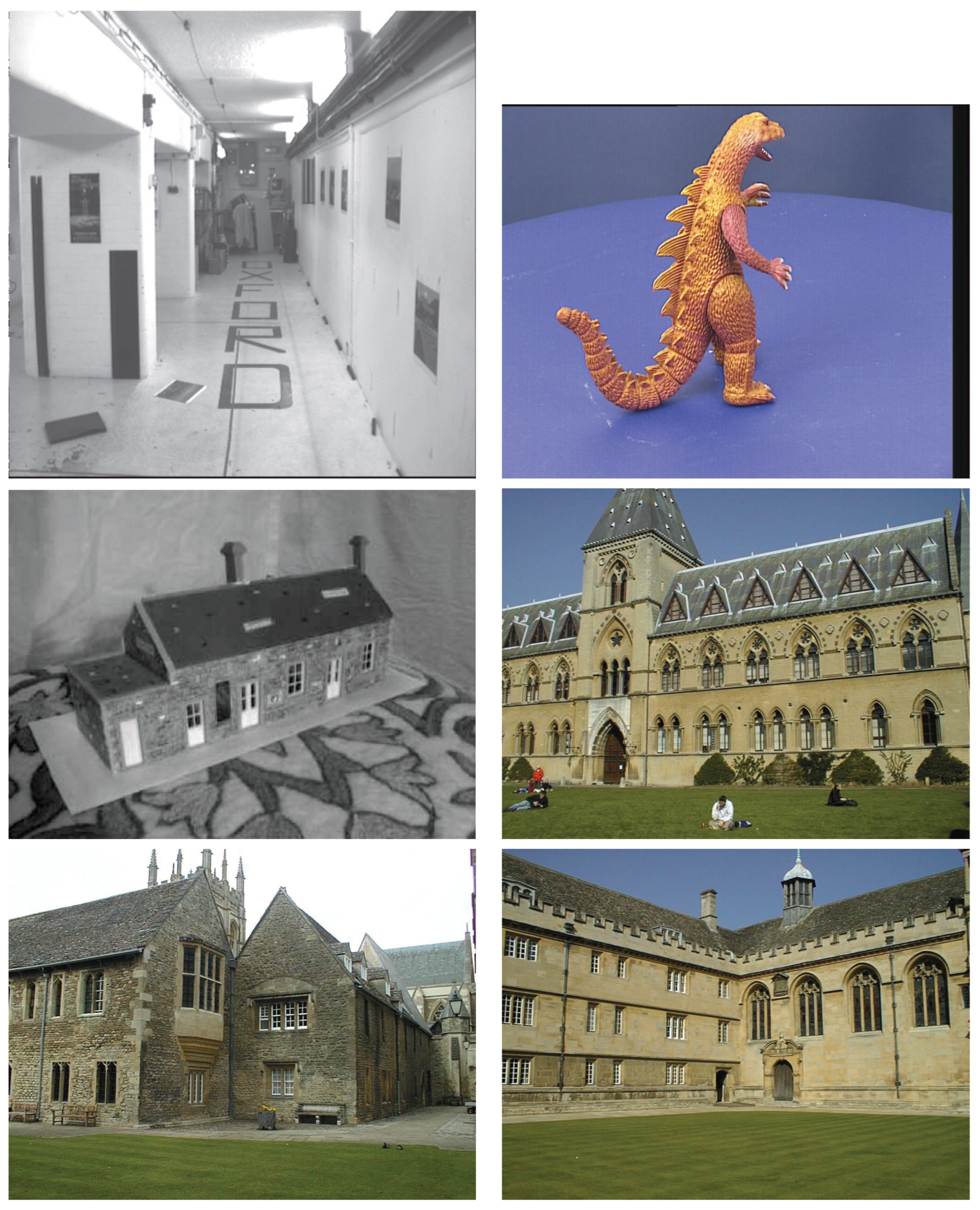
Here we present the results obtained with real data, in particular, using the following image sequences from the Visual Geometry Group at the University of Oxford:

• The corridor sequence (11 views with 737 points);
• The dinosaur sequence (36 views with 4983 points);
• The model house sequence (10 views with 672 points);
• The university library sequence (3 views with 667 points);
• The Merton College III sequence (3 views with 566 points);
• The Wadham College sequence (5 views with 1331 points).

• Only the points of these sequences visible in at least two views are here considered. Figure 2 shows an image of each sequence.

Each 3D point is estimated using all the available views through Corollary 1 with $\delta ={\delta }_{min}=2$. The estimations are carried out, firstly, by normalizing the data in order to improve the numerical accuracy, and, secondly, by de-normalizing the found solutions.

Table 1. Example 1: results for the corridor sequence found with Corollary 1 with $\delta ={\delta }_{min}=2$.

N	# Points Visible in	# Cases	$\mathit{mean}\left({\mathit{\gamma }}_{\mathit{UB}}\right)$	$\mathit{std}\left({\mathit{\gamma }}_{\mathit{UB}}\right)$	${\mathit{N}}_{\mathit{LMIVAR}}$	ACT [s]
	Exactly $\mathit{N}$ Views	${\mathit{\gamma }}_{\mathit{LB}}\ne {\mathit{\gamma }}_{\mathit{UB}}$
3	341	1	0.166	0.137	4	0.025
5	146	0	0.223	0.160	11	0.027
7	88	0	0.260	0.206	22	0.041
9	58	0	0.258	0.221	37	0.062
11	104	0	0.262	0.144	56	0.072

,

Table 2. Example 1: results for the dinosaur sequence found with Corollary 1 with $\delta ={\delta }_{min}=2$.

N	# Points Visible in	# Cases	$\mathit{mean}\left({\mathit{\gamma }}_{\mathit{UB}}\right)$	$\mathit{std}\left({\mathit{\gamma }}_{\mathit{UB}}\right)$	${\mathit{N}}_{\mathit{LMIVAR}}$	ACT [s]
	Exactly $\mathit{N}$ Views	${\mathit{\gamma }}_{\mathit{LB}}\ne {\mathit{\gamma }}_{\mathit{UB}}$
2	2300	0	0.121	0.104	2	0.015
3	1167	0	0.323	1.024	4	0.018
4	584	0	0.498	1.721	7	0.020
5	375	0	0.410	1.011	11	0.021
6	221	0	0.669	1.928	16	0.025
7	141	0	0.459	1.138	22	0.027
8	88	0	0.646	1.859	29	0.030
9	44	0	0.433	0.560	37	0.033
10	26	0	0.450	0.484	46	0.038
11	15	0	1.100	2.867	56	0.044
12	14	0	0.389	0.191	67	0.055
13	5	0	1.103	0.940	79	0.065
14	2	0	0.375	0.248	92	0.077
21	1	0	0.822	0.000	211	0.213

,

Table 3. Example 1: results for the model house sequence found with Corollary 1 with $\delta ={\delta }_{min}=2$.

N	# Points Visible in	# Cases	$\mathit{mean}\left({\mathit{\gamma }}_{\mathit{UB}}\right)$	$\mathit{std}\left({\mathit{\gamma }}_{\mathit{UB}}\right)$	${\mathit{N}}_{\mathit{LMIVAR}}$	ACT [s]
	Exactly $\mathit{N}$ Views	${\mathit{\gamma }}_{\mathit{LB}}\ne {\mathit{\gamma }}_{\mathit{UB}}$
3	382	0	0.209	0.143	4	0.020
4	19	0	0.372	0.125	7	0.027
5	158	0	0.294	0.506	11	0.022
6	3	0	0.625	0.237	16	0.016
7	90	0	0.374	0.320	22	0.030
8	1	0	0.686	0.000	29	0.032
9	12	0	0.476	0.270	37	0.045
10	7	0	0.266	0.104	46	0.052

,

Table 4. Example 1: results for the university library sequence found with Corollary 1 with $\delta ={\delta }_{min}=2$.

N	# Points Visible in	# Cases	$\mathit{mean}\left({\mathit{\gamma }}_{\mathit{UB}}\right)$	$\mathit{std}\left({\mathit{\gamma }}_{\mathit{UB}}\right)$	${\mathit{N}}_{\mathit{LMIVAR}}$	ACT [s]
	Exactly $\mathit{N}$ Views	${\mathit{\gamma }}_{\mathit{LB}}\ne {\mathit{\gamma }}_{\mathit{UB}}$
2	585	0	0.118	0.109	2	0.016
3	82	0	0.200	0.100	4	0.020

,

Table 5. Example 1: results for the Merton College III sequence found with Corollary 1 with $\delta ={\delta }_{min}=2$.

N	# Points Visible in	# Cases	$\mathit{mean}\left({\mathit{\gamma }}_{\mathit{UB}}\right)$	$\mathit{std}\left({\mathit{\gamma }}_{\mathit{UB}}\right)$	${\mathit{N}}_{\mathit{LMIVAR}}$	ACT [s]
	Exactly $\mathit{N}$ Views	${\mathit{\gamma }}_{\mathit{LB}}\ne {\mathit{\gamma }}_{\mathit{UB}}$
2	429	0	0.098	0.072	2	0.017
3	137	0	0.155	0.065	4	0.019

and

Table 6. Example 1: results for the Wadham College sequence found with Corollary 1 with $\delta ={\delta }_{min}=2$.

N	# Points Visible in	# Cases	$\mathit{mean}\left({\mathit{\gamma }}_{\mathit{UB}}\right)$	$\mathit{std}\left({\mathit{\gamma }}_{\mathit{UB}}\right)$	${\mathit{N}}_{\mathit{LMIVAR}}$	ACT [s]
	Exactly $\mathit{N}$ Views	${\mathit{\gamma }}_{\mathit{LB}}\ne {\mathit{\gamma }}_{\mathit{UB}}$
2	1052	0	0.098	0.077	2	0.017
3	215	0	0.143	0.063	4	0.022
4	50	0	0.157	0.055	7	0.020
5	14	0	0.165	0.030	11	0.024

show the obtained results.

As we can see from Table 1, Table 2, Table 3, Table 4, Table 5 and Table 6, ${\gamma }_{LB}$ is always equal to ${\gamma }_{UB}$, i.e., optimal, except for 1 point out of 8956 points. Specifically, this point belongs to the corridor sequence, and is visible in three views. The multiple-view $L_2$ triangulation problem for this point is (5)–(8) with

$$\left\{\begin{array}{ccccccc}\hfill {\widehat{\mathbf{P}}}_1& =& \left(\begin{array}{ccccccc}-736.733& ,& -13.521& ,& -388.497& ,& -828.164\\ -12.172& ,& -749.305& ,& -375.276& ,& -560.653\\ -0.029& ,& -0.062& ,& -1.469& ,& -3.214\end{array}\right)\hfill & ,& \hfill {\widehat{\mathcal{R}}}_1& =& \left(\begin{array}{c}375.782\\ 130.811\end{array}\right)\hfill \\ \hfill {\widehat{\mathbf{P}}}_2& =& \left(\begin{array}{ccccccc}-167.612& ,& -2.13& ,& -94.895& ,& -263.352\\ -2.619& ,& -171.436& ,& -86.19& ,& -185.115\\ -0.001& ,& -0.011& ,& -0.336& ,& -1.039\end{array}\right)\hfill & ,& \hfill {\widehat{\mathcal{R}}}_2& =& \left(\begin{array}{c}405.574\\ 129.657\end{array}\right)\hfill \\ \hfill {\widehat{\mathbf{P}}}_3& =& \left(\begin{array}{ccccccc}-176.193& ,& -1.451& ,& -108.707& ,& -381.816\\ -1.481& ,& -182.319& ,& -91.962& ,& -267.985\\ 0.009& ,& -0.01& ,& -0.357& ,& -1.478\end{array}\right)\hfill & ,& \hfill {\widehat{\mathcal{R}}}_3& =& \left(\begin{array}{c}443.672\\ 125.769\end{array}\right).\hfill \end{array}\right.$$

Using Corollary 1 with $\delta ={\delta }_{min}=2$ (for which $N_{LMIVAR}=4$), we obtain

$${\gamma }_{LB}=0.163,{\gamma }_{UB}=0.175,\widehat{\mathbf{X}}={(-3.869,4.736,-19.787)}^T$$

which does not allow us to conclude optimality of $\widehat{\mathbf{X}}$. However, using Corollary 1 with $\delta =4$ (for which $N_{LMIVAR}=281$) or Theorem 1 with $\delta ={\delta }_{min}=4$ (for which $N_{LMIVAR}=207$), we obtain

$${\gamma }_{LB}=0.170,{\gamma }_{UB}=0.170,\widehat{\mathbf{X}}={(-3.852,4.721,-19.722)}^T$$

which allows us to conclude optimality of $\widehat{\mathbf{X}}$.

Table 7. Results for Example 1 (see the beginning of Section 5 for the definitions of the abbreviations).

Method	# Cases	# Non-Optimal Cases	Optimality Recognized?	ACT [s]
Corollary 1	8956	1	yes for the	0.020
($\delta =2={\delta }_{min}$)			optimal cases
Newton	8956	4	NA	0.002
NMS	8956	11	NA	0.003
PSO	8956	5329	NA	0.299
SQP	8956	21	NA	0.010

reports the found results and the comparisons with the existing methods mentioned at the beginning of Section 5. As can be seen, the proposed approach (Corollary 1 with $\delta =2$), though slower than some of the existing methods, achieves the minimum number of non-optimal cases (one only, as previously explained). Moreover, only the proposed approach allows us to recognize the optimality of the found estimate.

5.2. Example 2

In this example, we consider a situation with three views where an admissible region is a circumference. Specifically, the uncertain multiple-view $L_2$ triangulation problem (5)–(8) is considered with

$$\left\{\begin{array}{ccccccc}\hfill {\widehat{\mathbf{P}}}_1& =& \left(\begin{array}{ccccccc}1& ,& 0& ,& 0& ,& 0\\ 0& ,& 1& ,& 0& ,& 0\\ 0& ,& 0& ,& 1& ,& 1\end{array}\right)\hfill & ,& \hfill {\widehat{\mathcal{R}}}_1& =& \left\{\mathbf{x}\in {\mathbb{R}}^2:{∥\mathbf{x}-\left(\begin{array}{c}0.8\\ 0.2\end{array}\right)∥}_2=1\right\}\hfill \\ \hfill {\widehat{\mathbf{P}}}_2& =& \left(\begin{array}{ccccccc}-1& ,& -1& ,& -1& ,& 0\\ 1& ,& 0& ,& -1& ,& 1\\ 1& ,& 0& ,& 1& ,& 1\end{array}\right)\hfill & ,& \hfill {\widehat{\mathcal{R}}}_2& =& \left(\begin{array}{c}0.4\\ -0.8\end{array}\right)\hfill \\ \hfill {\widehat{\mathbf{P}}}_3& =& \left(\begin{array}{ccccccc}0& ,& 1& ,& 0& ,& 0\\ 0& ,& 0& ,& 1& ,& -1\\ 1& ,& 1& ,& 0& ,& 1\end{array}\right)\hfill & ,& \hfill {\widehat{\mathcal{R}}}_3& =& \left(\begin{array}{c}-0.6\\ -1.8\end{array}\right).\hfill \end{array}\right.$$

Table 8. Results for Example 2 (see the beginning of Section 5 for the definitions of the abbreviations).

Method	${\widehat{\mathbf{X}}}^{\mathit{T}}$	$\mathit{\gamma }\left(\widehat{\mathbf{X}}\right)$	$\widehat{\mathbf{X}}$ Optimal?	${\mathit{N}}_{\mathit{LMIVAR}}$	CT [s]
			Optimality
			Recognized?
Theorem 1	$(-0.815,-0.070,0.793)$	0.412	yes, yes	676	0.968
($\delta =4={\delta }_{min}$)
Corollary 1	$(-0.747,-0.177,0.890)$	0.828	no, no	5	0.124
($\delta =2={\delta }_{min}$)
Corollary 1	$(-0.815,-0.070,0.793)$	0.412	yes, yes	721	1.066
($\delta =4$)
Newton	NA	NA	NA, NA	NA	NA
NMS	$(-0.815,-0.070,0.793)$	0.412	yes, NA	NA	0.030
PSO	$(-0.815,-0.070,0.793)$	0.412	yes, NA	NA	4.886
SQP	$(-0.815,-0.070,0.793)$	0.412	yes, NA	NA	0.046
TPML	$(-0.792,-0.109,0.821)$	0.459	no, no	829	1.555
(degree = 4)
TPML	?	?	?	14652	?
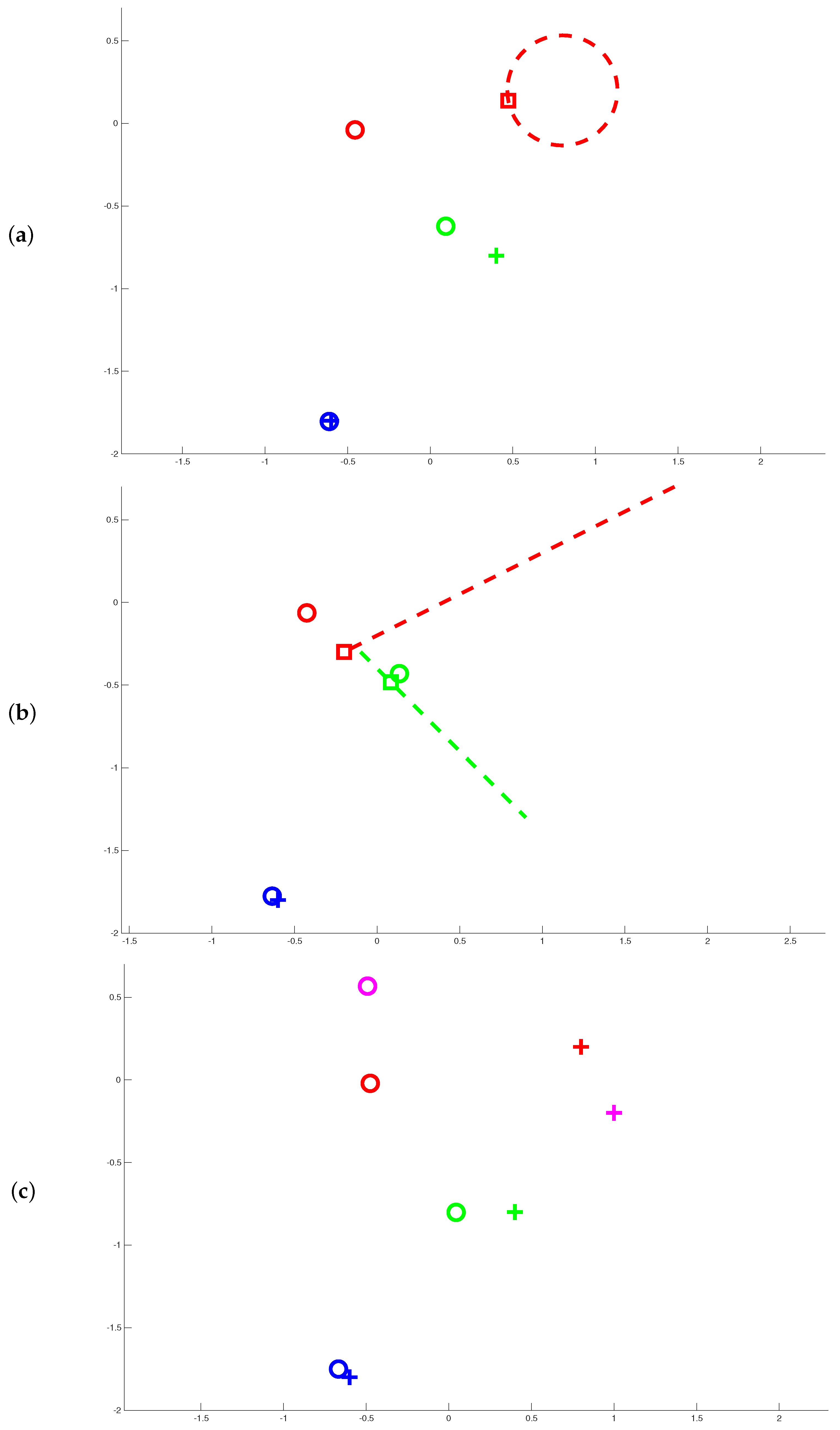
(degree = 6)					OOM

reports the found results and the comparisons with the existing methods mentioned at the beginning of Section 5. As can be seen, the optimal estimate is found by the proposed approach (Theorem 1 or Corollary 1 with $\delta =4$) and by the NMS, PSO and SQP methods. However, only the proposed approach allows us to recognize its optimality. Figure 3a shows the admissible regions ${\widehat{\mathcal{R}}}_i$ and the found image projections ${\mathbf{x}}_i^{*}$ in ${\mathbf{v}}^{*}$.

5.3. Example 3

In this example, we consider a situation with three views where two admissible regions are line segments. Specifically, the uncertain multiple-view $L_2$ triangulation problem (5)–(8) is considered with ${\widehat{\mathbf{P}}}_1$, ${\widehat{\mathbf{P}}}_2$ and ${\widehat{\mathbf{P}}}_3$ as in Example 2, and with

$$\left\{\begin{array}{ccc}\hfill {\widehat{\mathcal{R}}}_1& =& \left\{\left(\begin{array}{c}0.8\\ 0.2\end{array}\right)+{\mathbf{y}}_1\left(\begin{array}{c}1\\ 0.5\end{array}\right):{\mathbf{y}}_1\in [-1,1]\right\}\hfill \\ \hfill {\widehat{\mathcal{R}}}_2& =& \left\{\left(\begin{array}{c}0.4\\ -0.8\end{array}\right)+{\mathbf{y}}_2\left(\begin{array}{c}-0.5\\ 0.5\end{array}\right):{\mathbf{y}}_2\in [-1,1]\right\}\hfill \\ \hfill {\widehat{\mathcal{R}}}_3& =& \left(\begin{array}{c}-0.6\\ -1.8\end{array}\right).\hfill \end{array}\right.$$

Table 9. Results for Example 3 (see the beginning of Section 5 for the definitions of the abbreviations).

Method	${\widehat{\mathbf{X}}}^{\mathit{T}}$	$\mathit{\gamma }\left(\widehat{\mathbf{X}}\right)$	$\widehat{\mathbf{X}}$ Optimal?	${\mathit{N}}_{\mathit{LMIVAR}}$	CT [s]
			Optimality
			Recognized?
Theorem 1	$(-0.722,-0.108,0.698)$	0.138	yes, yes	721	1.216
($\delta =4={\delta }_{min}$)
Corollary 1	$(-0.685,-0.268,0.864)$	2.171	no, no	6	0.145
($\delta =2={\delta }_{min}$)
Corollary 1	$(-0.722,-0.108,0.698)$	0.138	yes, yes	766	1.283
($\delta =4$)
Newton	NA	NA	NA, NA	NA	NA
NMS	$(-0.744,-0.099,0.721)$	0.139	no, NA	NA	0.038
PSO	$(-1.665,-1.670,5.114)$	0.656	no, NA	NA	2.092
SQP	$(-0.722,-0.108,0.698)$	0.138	yes, NA	NA	0.051
TPML	$(-0.710,-0.133,0.725)$	0.166	no, no	874	2.418
(degree = 4)
TPML	?	?	?	16227	?
(degree = 6)					OOM

reports the found results and the comparisons with the existing methods mentioned at the beginning of Section 5. As can be seen, the optimal estimate is found by the proposed approach (Theorem 1 or Corollary 1 with $\delta =4$) and by the SQP method. However, only the proposed approach allows us to recognize its optimality. Figure 3b shows the admissible regions ${\widehat{\mathcal{R}}}_i$ and the found image projections ${\mathbf{x}}_i^{*}$ in ${\mathbf{v}}^{*}$.

5.4. Example 4

In this example, we consider a situation with four views. Specifically, the uncertain multiple-view $L_2$ triangulation problem (5)–(8) is considered with ${\widehat{\mathbf{P}}}_1$, ${\widehat{\mathbf{P}}}_2$ and ${\widehat{\mathbf{P}}}_3$ as in Example 2, and with

$$\left\{\begin{array}{c}{\widehat{\mathbf{P}}}_4=\left(\begin{array}{ccccccc}1& ,& -1& ,& 0& ,& 0\\ 1& ,& 0& ,& 1& ,& 1\\ 0& ,& 1& ,& 2& ,& 0\end{array}\right)\\ {\widehat{\mathcal{R}}}_1=\left(\begin{array}{c}0.8\\ 0.2\end{array}\right),{\widehat{\mathcal{R}}}_2=\left(\begin{array}{c}0.4\\ -0.8\end{array}\right),{\widehat{\mathcal{R}}}_3=\left(\begin{array}{c}-0.6\\ -1.8\end{array}\right),{\widehat{\mathcal{R}}}_4=\left(\begin{array}{c}1\\ -0.2\end{array}\right).\end{array}\right.$$

Table 10. Results for Example 4 (see the beginning of Section 5 for the definitions of the abbreviations).

Method	${\widehat{\mathbf{X}}}^{\mathit{T}}$	$\mathit{\gamma }\left(\widehat{\mathbf{X}}\right)$	$\widehat{\mathbf{X}}$ Optimal?	${\mathit{N}}_{\mathit{LMIVAR}}$	CT [s]
			Optimality
			Recognized?
Theorem 1	$(-0.901,-0.039,0.897)$	0.760	yes, yes	591	1.308
($\delta =4={\delta }_{min}$)
Corollary 1	$(-0.921,-0.650,1.784)$	0.925	no, no	7	0.139
($\delta =2={\delta }_{min}$)
Corollary 1	$(-0.901,-0.039,0.897)$	0.760	yes, yes	811	1.442
($\delta =4$)
Newton	$(-84.55,1387,-414.2)$	2.049	no, NA	NA	0.004
NMS	$(-0.849,0.493,-0.571)$	1.597	no, NA	NA	0.006
PSO	$(-13.58,-44.31,100)$	0.824	no, NA	NA	0.098
SQP	$(-100,-22.31,-77.22)$	1.215	no, NA	NA	0.025
TPML	$(-0.979,-0.975,2.136)$	0.901	no, no	1259	4.396
(degree = 4)
TPML	?	?	?	22303	?
(degree = 6)					OOM

reports the found results and the comparisons with the existing methods mentioned at the beginning of Section 5. As can be seen, only the proposed approach (Theorem 1 or Corollary 1 with $\delta =4$) allows to find the optimal estimate and to recognize its optimality. Figure 3c shows the admissible regions ${\widehat{\mathcal{R}}}_i$ and the found image projections ${\mathbf{x}}_i^{*}$ in ${\mathbf{v}}^{*}$.

5.5. Example 5

In this last example, we aim to investigate multiple trials for acquiring the estimates of the image projections and of the projection matrices with the same level of the uncertainty, as well as investigating the obtained results for different levels of the uncertainty. To this end, we generate a total of 1000 cases, as follows:

• Firstly, we randomly generate 25 scene points ${\mathbf{X}}_{obj}$ visible in the four views described by the projection matrices ${\mathbf{P}}_1,\dots ,{\mathbf{P}}_4$ chosen as the projection matrices used in Example 4 and normalized in order to have unitary 2-norm;
• Secondly, for each scene point, we calculate its image projections ${\mathbf{x}}_1,\dots ,{\mathbf{x}}_4$ in the four views;
• Thirdly, we consider four different levels of the uncertainty parameterized by the scalar $\theta$ according to $\theta =0.05,0.1,0.15,0.2$;
• Fourthly, for each scene point and for each level of the uncertainty, we generate, over 10 times (the trials), the following:

  –

  The estimates ${\widehat{\mathcal{R}}}_i,\dots ,{\widehat{\mathcal{R}}}_4$ of the image projections of the scene point by adding a random uncertainty in the interval $[-\theta A,\theta A]$ to each entry of the true image projections ${\mathbf{x}}_1,\dots ,{\mathbf{x}}_4$, where $A={max}_{i=1,\dots ,4}{\parallel {\mathbf{x}}_i\parallel }_2$;

  –

  The estimates ${\widehat{\mathbf{P}}}_1,\dots ,{\widehat{\mathbf{P}}}_4$ of the projection matrices by adding a random uncertainty in the interval $[-\theta ,\theta ]$ to each entry of the true projection matrices.

Table 11. Results for Example 5 part 1 (see the beginning of Section 5 for the definitions of the abbreviations).

Method	# Non-Optimal Cases for				Optimality	${\mathit{N}}_{\mathit{LMIVAR}}$	ACT [s]
	$\mathit{\theta }=\mathbf{0.05}$	$\mathit{\theta }=\mathbf{0.1}$	$\mathit{\theta }=\mathbf{0.15}$	$\mathit{\theta }=\mathbf{0.2}$	Recognized?
Theorem 1	0	0	0	0	yes	591	0.892
($\delta =4={\delta }_{min}$)
Corollary 1	0	0	6	41	yes for the	7	0.023
($\delta =2={\delta }_{min}$)					optimal cases
Corollary 1	0	0	0	0	yes	811	1.013
($\delta =4$)
Newton	1	17	37	71	NA	NA	0.002
NMS	0	0	2	7	NA	NA	0.004
PSO	23	22	33	47	NA	NA	0.338
SQP	0	0	1	6	NA	NA	0.009
TPML	0	0	6	40	yes for the	1259	1.811
(degree = 4)					optimal cases
TPML	?	?	?	?	?	22303	?
(degree = 6)							OOM

and

Table 12. Results for Example 5 part 2 (see the beginning of Section 5 for the definitions of the abbreviations).

Method	Average Distance from $\widehat{\mathbf{X}}$ to ${\mathbf{X}}_{\mathit{obj}}$ for
	$\mathit{\theta }=\mathbf{0.05}$	$\mathit{\theta }=\mathbf{0.1}$	$\mathit{\theta }=\mathbf{0.15}$	$\mathit{\theta }=\mathbf{0.2}$
Theorem 1	0.195	0.387	0.543	0.846
($\delta =4={\delta }_{min}$)
Corollary 1	0.195	0.387	0.543	1.070
($\delta =2={\delta }_{min}$)
Corollary 1	0.195	0.387	0.543	0.846
($\delta =4$)
Newton	0.205	6.773	13.29	27.25
NMS	0.195	0.387	0.553	1.542
PSO	3.393	4.233	8.844	6.771
SQP	0.195	0.387	0.594	1.932
TPML	0.195	0.387	0.710	1.075
(degree = 4)
TPML	?	?	?	?
(degree = 6)				OOM

report the found results and the comparisons with the existing methods mentioned at the beginning of Section 5. As can be seen, only the proposed approach (Theorem 1 or Corollary 1 with $\delta =4$) achieves zero non-optimal cases, allows us to recognize the optimality of the found solution, and achieves the minimum average distance from the estimated scene point to the true one.

6. Conclusions

This paper has proposed a novel approach for uncertain multiple-view $L_2$ triangulation where the estimated image projections are allowed to be uncertain in admissible regions described by polynomial inequalities and equalities. The proposed approach is based on the introduction of polynomial multipliers and requires the solution of an LMI problem. It has been proven that the optimal estimate of the scene point can always be achieved by using multipliers with sufficiently large degree. Moreover, a simple test has been provided in order to establish the optimality of the found estimate.

The complexity of the proposed approach has been investigated by deriving analytical expressions for the number of independent LMI scalar variables present in the derived LMI problems. Although these expressions show that this number may quickly grow with the number of views and with the number and degree of the polynomials involved, various examples with real and synthetic data have shown that the complexity is not only manageable but also competitive at least with respect to the existing methods based on convex optimization.

The proposed approach presents key advantages with respect to several existing methods of a different nature. Indeed, various examples with real and synthetic data have shown that the existing methods based on nonconvex optimization may fail to find the optimal estimate or may not allow one to establish the optimality of the found estimate, while the existing methods based on convex optimization may fail to find the optimal estimate or may require a larger computational burden.

Future work could consider reducing the complexity of the proposed approach (for instance, by exploiting KKT conditions or duality theory), integrating the proposed approach with methods for camera pose estimation, and developing an open-source code of the proposed approach.

References

1. Hartley, R.; Zisserman, A. Multiple View in Computer Vision; Cambridge University Press: New York, NY, USA, 2000. [Google Scholar]
2. Torralba, A.; Isola, P.; Freeman, W. Foundations of Computer Vision; MIT Press: Cambridge, UK, 2024. [Google Scholar]
3. Hartley, R.; Schaffalitzky, F. L minimization in geometric reconstruction problems. In Proceedings of the IEEE Conference on Computer Vision and Pattern Recognition, Washington, DC, USA, 27 June–2 July 2004; pp. 504–509. [Google Scholar]
4. Ke, Q.; Kanade, T. Uncertainty models in quasiconvex optimization for geometric reconstruction. In Proceedings of the IEEE Conference on Computer Vision and Pattern Recognition, New York, NY, USA, 17–22 June 2006; pp. 1199–1205. [Google Scholar]
5. Zhang, L.; Zhang, J.; Hu, Y. Triangulation in omnidirectional vision under the L-norm. In Proceedings of the IEEE International Conference on Information and Automation, Harbin, China, 20–23 June 2010; pp. 1757–1762. [Google Scholar]
6. Stewenius, H.; Schaffalitzky, F.; Nister, D. How hard is 3-view triangulation really? In Proceedings of the International Conference on Computer Vision, Beijing, China, 17–20 October 2005; pp. 686–693. [Google Scholar]
7. Lu, F.; Hartley, R. A fast optimal algorithm for L2 triangulation. In Proceedings of the Asian Conference on Computer Vision, Tokyo, Japan, 18–22 November 2007; Volume 4844, pp. 279–288. [Google Scholar]
8. Nair, N.S.; Nair, M.S. On evolutionary computation techniques for multi-view triangulation. Mach. Vis. Appl. 2020, 31, 29. [Google Scholar] [CrossRef]
9. Rydell, F.; Bokman, G. A framework for reducing the complexity of geometric vision problems and its application to two-view triangulation with approximation bounds. In Proceedings of the International Conference on 3D Vision, Vancouver, BC, Canada, 20–23 March 2026; pp. 257–266. [Google Scholar]
10. Boyd, S.; Vandenberghe, L. Convex Optimization; Cambridge University Press: Cambridge, UK, 2004. [Google Scholar]
11. Hendrix, E.M.T.; Toth, B.G. Introduction to Nonlinear and Global Optimization; Springer: Berlin/Heidelberg, Germany, 2010. [Google Scholar]
12. Grippo, L.; Sciandrone, M. Introduction to Methods for Nonlinear Optimization; Springer: Berlin/Heidelberg, Germany, 2023. [Google Scholar]
13. Chesi, G.; Hung, Y.S. Fast multiple-view L2 triangulation with occlusion handling. Comput. Vis. Image Underst. 2011, 115, 211–223. [Google Scholar] [CrossRef]
14. Chesi, G. On the complexity of SOS programming and applications in control systems. Asian J. Control 2018, 20, 2005–2013. [Google Scholar]
15. Gisleris, E.; Serackis, A. Enhancing 3D pose estimation accuracy from multiple camera perspectives through machine learning model integration. In Proceedings of the IEEE Jubilee Workshop on Advances in Information, Electronic and Electrical Engineering, Vilnius, Lithuania, 27–29 April 2023; pp. 1–4. [Google Scholar]
16. Lin, X.; Zhou, Y.; Zhang, X.; Liu, Y.; Zhu, C. Efficient and effective multi-camera pose estimation with weighted M-estimate sample consensus. In Proceedings of the IEEE International Conference on Acoustics, Speech and Signal Processing, Rhodes Island, Greece, 4–10 June 2023; pp. 1–5. [Google Scholar]
17. Skarbek, W.; Salamonowicz, M.; Krol, M. Camera pose revisited. Appl. Sci. 2026, 16, 2690. [Google Scholar] [CrossRef]
18. Hwang, T.; Kim, M. Noise-robust 3D pose estimation using appearance similarity based on the distributed multiple views. Sensors 2024, 24, 5645. [Google Scholar] [CrossRef] [PubMed]
19. Chen, M.; Tan, G. 3D human pose estimation based on wearable IMUs and multiple camera views. Electronics 2024, 13, 2926. [Google Scholar] [CrossRef]
20. Konyashov, V.V.; Sergeev, A.S.; Kolganov, O.A.; Fedorov, A.V.; Konyashova, K.A.; Bychenok, V.V. Study of the applicability of the method of optical triangulation for evaluation of the geometric parameters and cleanliness of the surface of products of complex shapes. In Proceedings of the International Conference on Information, Control, and Communication Technologies, Astrakhan, Russia, 2–6 October 2023; pp. 1–6. [Google Scholar]
21. Kim, J.W.; Ha, J.E. End-to-end camera pose estimation with camera ray token. Electronics 2025, 14, 4624. [Google Scholar] [CrossRef]
22. Ding, G.; Chen, T.; Sun, L.; Fan, P. High precision camera calibration method based on full camera model. In Proceedings of the Chinese Control and Decision Conference, Xi’an, China, 25–27 May 2024; pp. 4218–4223. [Google Scholar]
23. Dhatrak, S.; Kumar, S.; Shah, A.; Gupta, A. Stereo calibration of heterogeneous RGB-ToF camera for robotics applications. In Proceedings of the International Conference on Artificial Intelligence, Robotics and Control, Savannah, GA, USA, 9–11 April 2025; pp. 23–28. [Google Scholar]
24. Hung, C.W.; Chang, T.A.; Chen, X.N.; Wang, C.C. Monocular camera pose estimation and calibration system based on raspberry Pi. Electronics 2025, 14, 3694. [Google Scholar] [CrossRef]
25. Li, L.; Xiao, Z.; Hu, T. Camera Calibration optimization algorithm based on nutcracker optimization algorithm. Sensors 2025, 25, 3521. [Google Scholar] [CrossRef] [PubMed]
26. Hou, C.; He, Z.; Zhao, T.; Guo, Z.; Ji, X. Online extrinsic calibration of camera and LiDAR based on cascade optimization. Sensors 2026, 26, 2282. [Google Scholar] [CrossRef] [PubMed]
27. Scheiderer, C. A Course in Real Algebraic Geometry: Positivity and Sums of Squares; Springer: Berlin/Heidelberg, Germany, 2024. [Google Scholar]
28. Chesi, G. LMI-Based Robustness Analysis In Uncertain Systems; Foundations and Trends in Systems and Control; Now Publishers: Hanover, MA, USA, 2024. [Google Scholar]
29. Boyd, S.; El Ghaoui, L.; Feron, E.; Balakrishnan, V. Linear Matrix Inequalities in System and Control Theory; SIAM: Philadelphia, PA, USA, 1994. [Google Scholar]
30. Chesi, G. Domain of Attraction: Analysis and Control via SOS Programming; Springer: Berlin/Heidelberg, Germany, 2011. [Google Scholar]
31. Shami, T.M.; El-Saleh, A.A.; Alswaitti, M.; Al-Tashi, Q.; Summakieh, M.A.; Mirjalili, S. Particle swarm optimization: A comprehensive survey. IEEE Access 2022, 10, 10031–10061. [Google Scholar] [CrossRef]
Figure 1. An illustration of multiple-view triangulation, where a flower is observed by three cameras, and the scene point to be estimated is the center of the red portion.
Bdcc 10 00222 g001
Figure 2. Example 1: an image of each sequence.
Bdcc 10 00222 g002
Figure 3. Plots for Examples 2 (subfigure (a)), 3 (subfigure (b)) and 4 (subfigure (c)). The subfigures show the admissible regions R ^ i (denoted by the “+” markers and by the curves and lines) and the found image projections x i * (denoted by the “o” markers) for i = 1 (red), i = 2 (green), i = 3 (blue) and i = 4 (violet). The square markers in the subfigures (a,b) denote the closest points to x i * in the admissible regions R ^ i .
Bdcc 10 00222 g003