Towards an Ultra-High-Speed Combustion Pyrometer †


Abstract
:1. Introduction
2. System Design and Theoretical Model
- A sensor: a 2 m long gold-coated multi-mode (MM) step-index fibre, with 400 µm core diameter, numerical aperture NA = 0.22, stainless-steel monocoil sheathing, a sub-miniature (SMA) connector on one end (hot front end) and a fibre-channel (FC) connector on the other end (cold back end)—for testing purposes, this was placed inside a ~1.7 m long stainless-steel tube (outer diameter: 20 mm, inner diameter: 16 mm), with the SMA connector protected by a recessed sapphire window; sensor and packaging can be tailored to the final application and installation requirements (e.g., addition of a collimating lens).
- An extension lead fibre: a lightly-armoured 10 m long MM step-index fibre patch-cord, with 600 µm core diameter, NA = 0.22, dual acrylate coating, 3 mm diameter polyvinyl chloride (PVC) sleeve and FC connectors on both ends—this connects the sensor (on the FC connector) to the interrogator.
- A passive optoelectronic interrogator, assembled in-house and consisting mainly of:
- ○
- a custom-made 1 × 3 mm2 step-index fibre coupler/splitter with 600 µm core diameter, NA = 0.22 and FC connectors on all ports;
- ○
- three photodetector assemblies, using off-the-shelf components, for measuring optical thermal radiation at 3 different wavelengths: λ1 = 850 nm, λ2 = 1050 nm and λ3 = 1300 nm;
- ○
- a power supply unit to power the photodetectors.
- A National Instrument (NI) data acquisition (DAQ) system, with maximum sampling rate fMAX = 1 MHz, connected to the optoelectronic interrogator via BNC cables and to a Personal Computer (PC) via a USB cable.
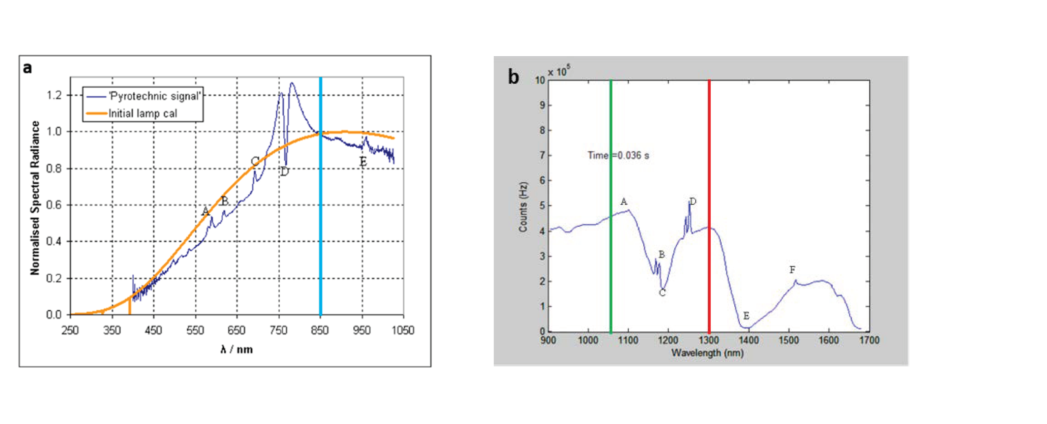
- 589 nm—Sodium (Na) emission lines;
- 619 nm—CaOH emission lines;
- 693 nm—Potassium (K) emission lines;
- 767 nm—K emission and absorption lines;
- 960 nm—Uncertain of assignment.
- 1104 nm—K emission lines;
- 1169 nm—K emission lines;
- Broad OH absorption in the fibre;
- 1243 and 1252 nm—K emission lines;
- Broad OH absorption in the fibre;
- 1517 nm—K emission lines.
- T is the blackbody temperature in K;
- σ = 5.67 × 10⁻⁸ W·m−2·K−4 is the Stefan–Boltzmann constant;
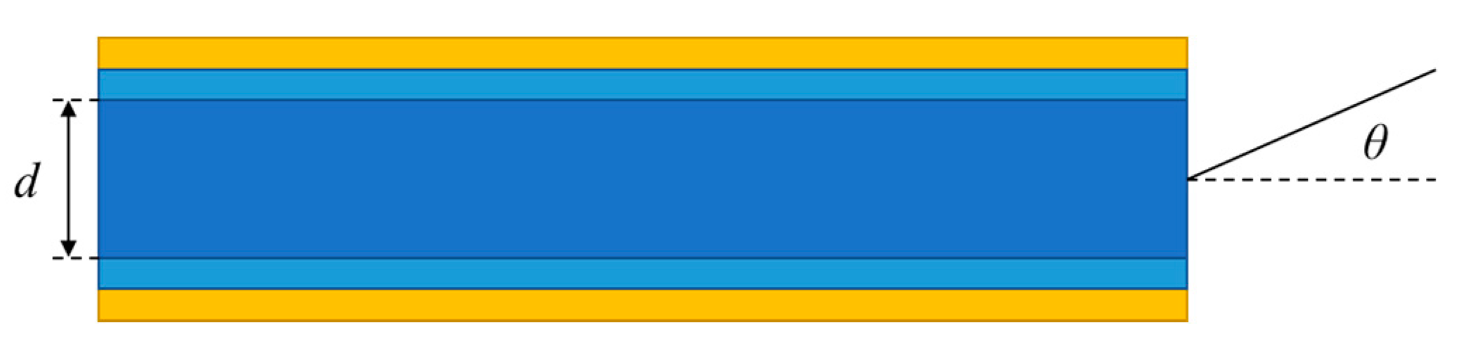
- A = πd2/4 = 1.25664 × 10⁻⁷ m2 is the fibre core area;
- Ω = πtan2(θ) is the maximum solid acceptance angle of the Au-coated fibre, with θ the maximum acceptance half-angle of the Au-coated fibre, which is related to the NA of the fibre as: NA = nsin(θ) = 0.22
- The transmission factor of the sapphire window placed in front of the fibre end-facet, due to Fresnel reflection losses (7% at each interface/surface): t0 = 0.93 × 0.93 = 0.8649.
- The transmission factor at the end-facet of the Au-coated fibre, due to Fresnel reflection losses: t1 = 0.96.
- Transmission losses of 12 m of fibre (2 m sensor + 10 m of extension lead fibre)—considering that typical losses for large-core multi-mode fibre are of the order of 10 dB/km or less at λ = (0.6–1.6) μm: tfibre = −0.12 dB ≈ 0.973.
- Losses due to optical connectors (3), typically of the order of 0.3 dB each—i.e., a transmission factor tconnector = 0.933
- The splitting ratio of the 1 × 3 optical coupler/splitter: tsplitter ≈ 0.333.
- The optical transmission (tfilter) of the bandpass filters in the photodetector assemblies—it is worth noting that the filters used have different values of optical transmission peak and Full-Width-at-Half Maximum (FWHM):
- ○
- t850 nm = 70%;
- ○
- t1050 nm = 45%;
- ○
- t1300 nm = 40%;
- ○
- FWHM850 nm = 40 nm ± 8 nm;
- ○
- FWHM1050 nm = 10 nm ± 2 nm;
- ○
- FWHM1300 nm = 30 nm ± 6 nm.
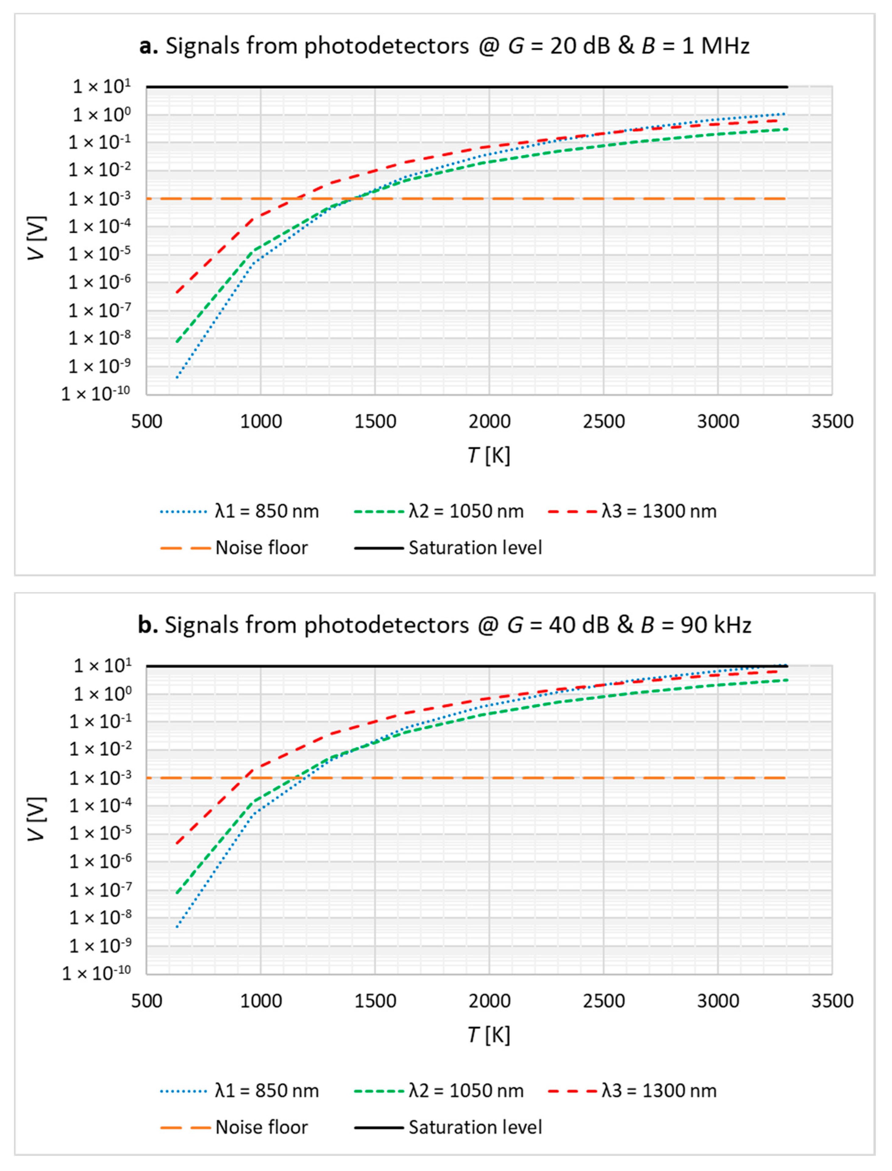
- With a gain of G = 20 dB (B = 1 MHz—Figure 5a), the instrument can measure a minimum temperature of ~1150 K at a single wavelength (λ3 = 1300 nm) or ~1400 K at all three wavelengths.
- With a gain of G = 30 dB (B = 260 kHz), the minimum measurable temperature can be brought down to ~1025 K for single-wavelength measurement (λ3 = 1300 nm) and ~1275 K at all three wavelengths, but at cost of reduced sampling speed (f ≤ B = 260 kHz), while still avoiding saturation at 3300 K, our maximum temperature of interest.
- With a gain of G ≥ 40 dB (B = 90 kHz—Figure 5b), the photodetectors would start saturating at TMAX < 3300 K and their bandwidth would decrease significantly, down to B = 3 kHz at G = 70 dB.
3. Instrument Calibration
3.1. Test Rig
3.2. Test Method
- The blackbody furnace was set at the required temperature set-point.
- The temperature of the blackbody cavity was monitored using the LP3.
- Once the blackbody temperature reached stability, a measurement was taken from the LP3, by measuring the average and standard deviation over ~30 s (the LP3 is sampled at 1 Hz).
- The LP3 was moved out of the way and the sensor moved into place, so that it was in line with and parallel to the long axis of the blackbody, as shown in Figure 6.
- Data acquisition and logging were started on the instrument.
- Manually, the sensor was quickly moved into and out of the blackbody (within a few seconds).
- Two measurements were made at each set-point temperature.
3.3. Test Data Analysis Method
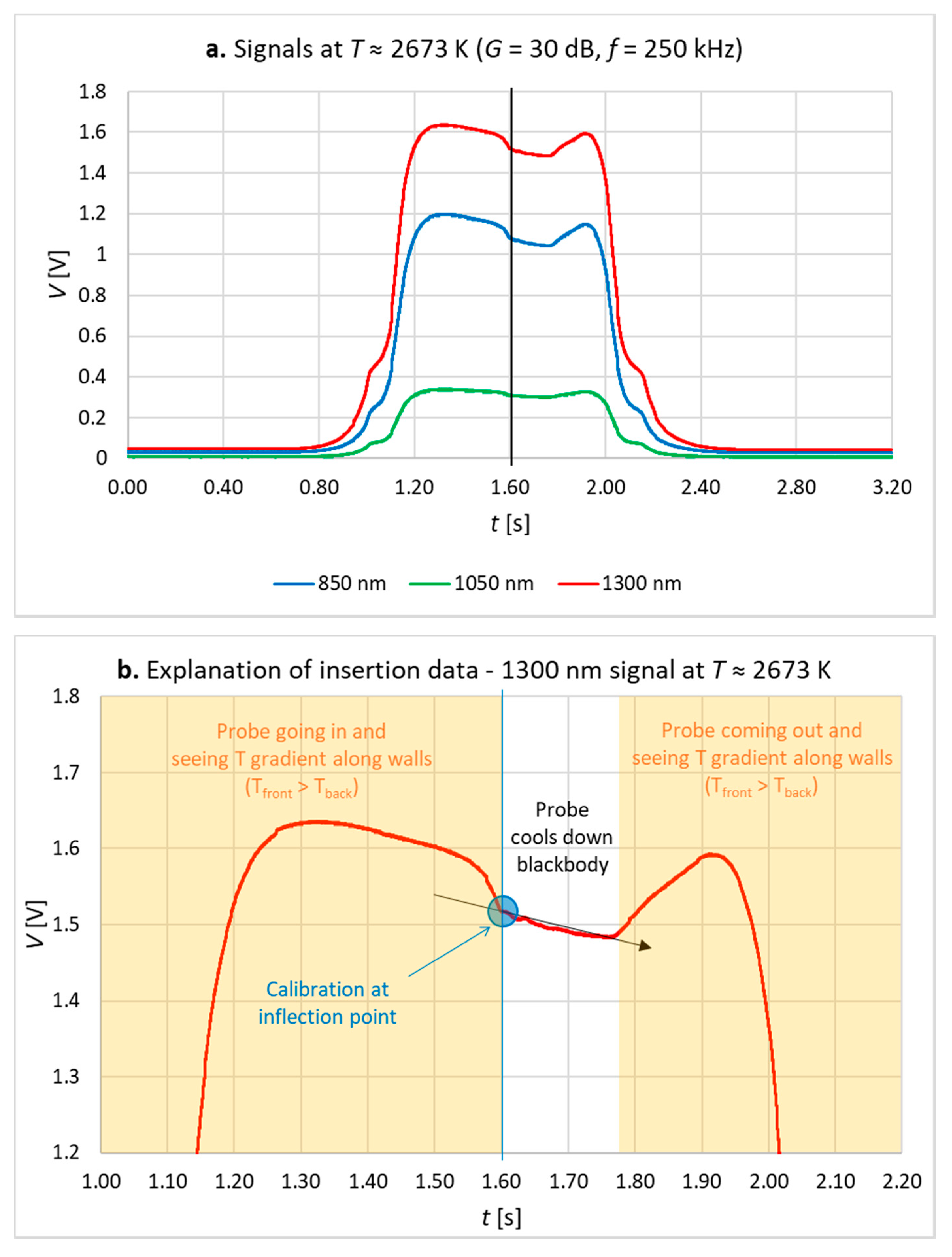
- t < 1.3 s: the blackbody cavity had a temperature gradient along the cavity wall and across its rear surface, it was hotter to the outside, and this was seen as the sensor approached: the radiance signal increased as the field of view of the sensor was initially filled.
- t ≈ (1.3–1.6) s: the signal fell as the sensor progressively saw more of the cooler central section of the back wall.
- t ≈ (1.6–1.77) s: there was a period when the blackbody temperature fell due to heat lost to the cold sensor.
- t ≈ (1.77–1.92) s: as the sensor was withdrawn, the hotter regions of the blackbody cavity were seen again, so that the signal increased.
- t > 1.92 s: the signal decreased, as the sensor was withdrawn from the blackbody cavity.
- The maximum in the signal during sensor removal was lower than during insertion. This is consistent with the cooling of the blackbody cavity.
- The voltages recorded for calibration were chosen at the inflection point of each signal, highlighted by the blue circle, as it corresponds to the point when the field of view of the fibre is filled with thermal radiation from the back wall, before any further cooling caused by the sensor.
3.4. Calibration Test Results
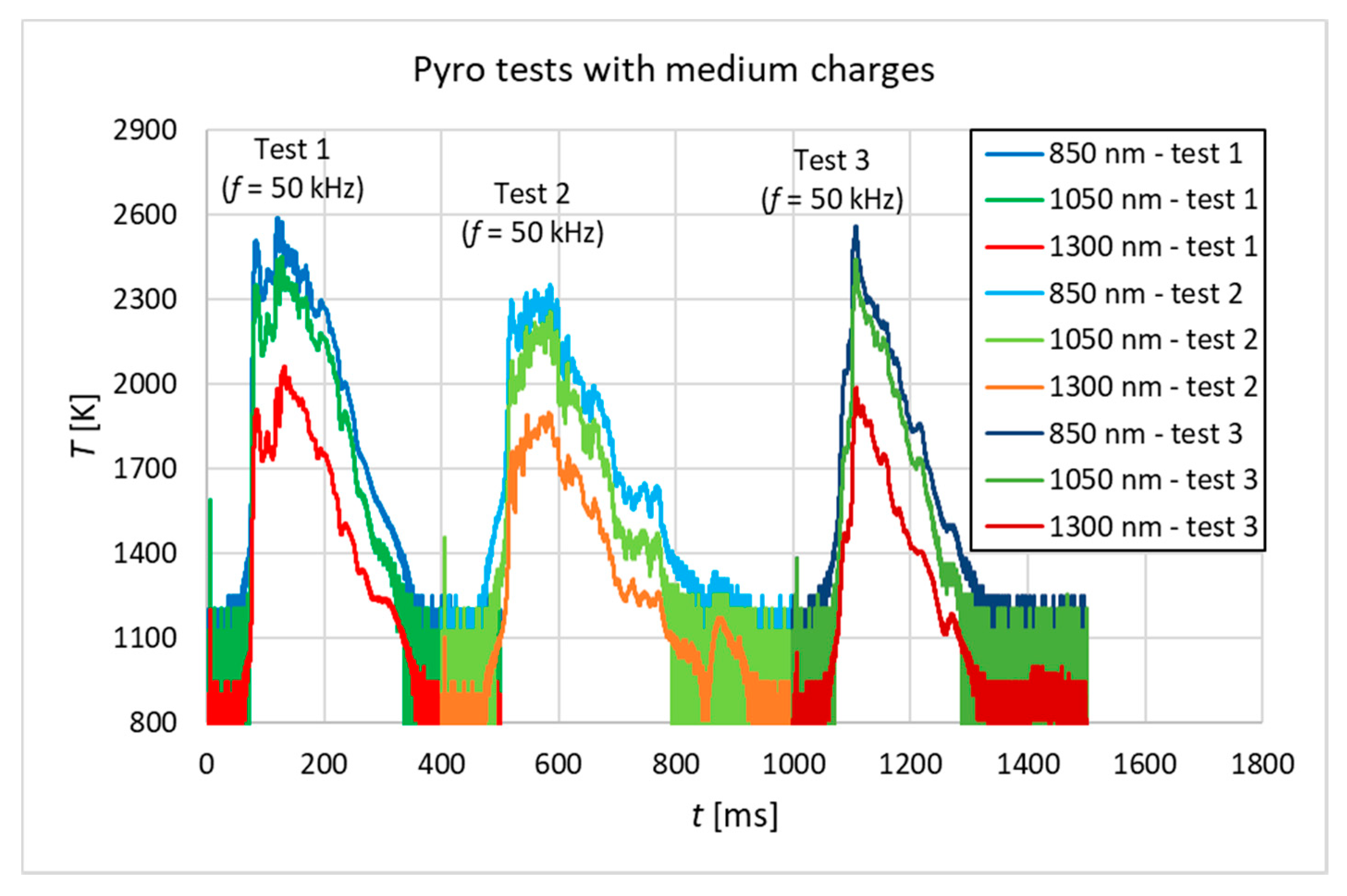
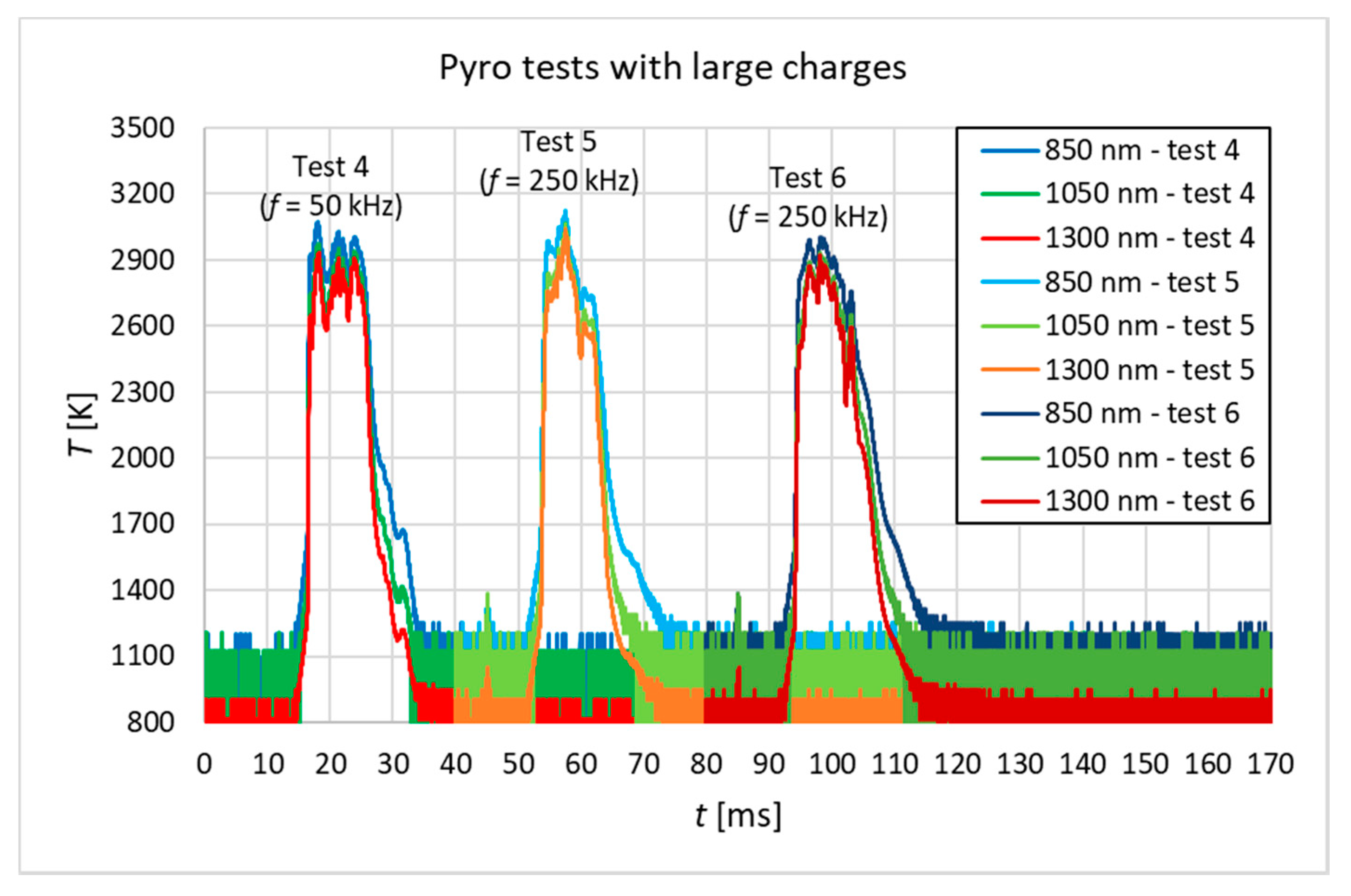
4. Dynamic Tests
4.1. Test Rig
4.2. Test Method
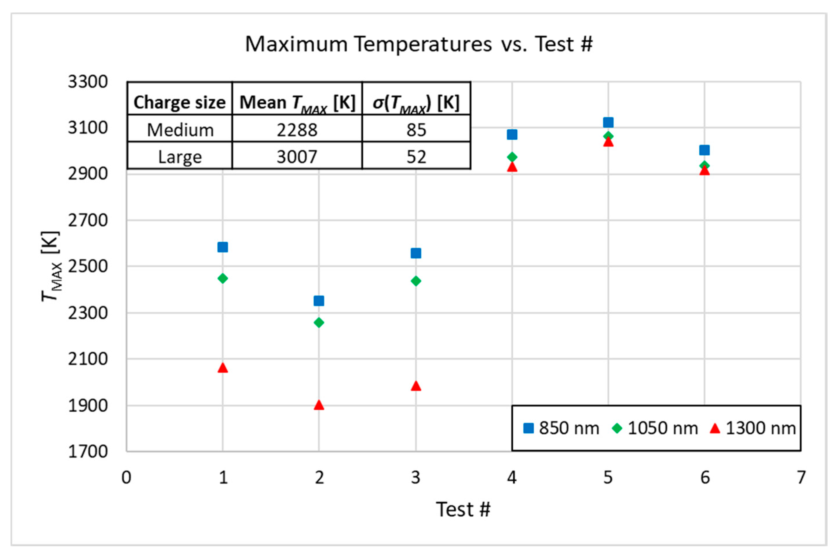
4.3. Test Results
5. Conclusions
Author Contributions
Funding
Conflicts of Interest
References
- Teichmann, R.; Wimmer, A.; Schwarz, C.; Winklhofer, E. Combustion Diagnostic. In Combustion Engines Development—Mixture Formation, Combustion, Emissions and Simulation; Merker, G.P., Schwarz, C., Teichmann, R., Eds.; Springer: Berlin/Heidelberg, Germany, 2012; p. 115. [Google Scholar]
- Saxholm, S.; Högström, R.; Sarraf, C.; Sutton, G.; Wynands, R.; Arrhén, F.; Jönsson, G.; Durgut, Y.; Peruzzi, A.; Fateev, A. Development of measurement and calibration techniques for dynamic pressures and temperatures (DynPT): Background and objectives of the 17IND07 DynPT project in the European Metrology Programme for Innovation and Research (EMPIR). J. Phys. Conf. Ser. 2018, 1065, 162015. [Google Scholar] [CrossRef]
- Preston-Thomas, H. The International Temperature Scale of 1990 (ITS-90). Metrologia 1990, 27, 3–10. [Google Scholar] [CrossRef]
- Saunders, P.; White, D.R. Physical basis of interpolation equations for radiation thermometry. Metrologia 2003, 40, 195–203. [Google Scholar] [CrossRef]
- Safety Datasheet of LeMaitre Ltd. Theatrical Flashes. Available online: https://www.lemaitreltd.com/products/pyrotechnics/pyroflash/theatrical-flashes-stars/theatrical-flashes/sds-flashes-robotics-spds/ (accessed on 22 November 2020).


| λi [nm] | Ai [V] | ci [µm K] |
|---|---|---|
| 850 | 527.6 | 14,082.2 |
| 1050 | 53.0 | 14,431.8 |
| 1300 | 91.7 | 14,307.3 |
| λi [nm] | TMIN [K] | TMAX [K] |
|---|---|---|
| 850 | 1260 | 4160 |
| 1050 | 1260 | 7470 |
| 1300 | 960 | 4740 |
Publisher’s Note: MDPI stays neutral with regard to jurisdictional claims in published maps and institutional affiliations. |
© 2020 by the authors. Licensee MDPI, Basel, Switzerland. This article is an open access article distributed under the terms and conditions of the Creative Commons Attribution (CC BY-NC-ND) license (http://creativecommons.org/licenses/by-nc-nd/4.0/).
Share and Cite
Sposito, A.; Lowe, D.; Sutton, G. Towards an Ultra-High-Speed Combustion Pyrometer. Int. J. Turbomach. Propuls. Power 2020, 5, 31. https://doi.org/10.3390/ijtpp5040031
Sposito A, Lowe D, Sutton G. Towards an Ultra-High-Speed Combustion Pyrometer. International Journal of Turbomachinery, Propulsion and Power. 2020; 5(4):31. https://doi.org/10.3390/ijtpp5040031
Chicago/Turabian StyleSposito, Alberto, Dave Lowe, and Gavin Sutton. 2020. "Towards an Ultra-High-Speed Combustion Pyrometer" International Journal of Turbomachinery, Propulsion and Power 5, no. 4: 31. https://doi.org/10.3390/ijtpp5040031
APA StyleSposito, A., Lowe, D., & Sutton, G. (2020). Towards an Ultra-High-Speed Combustion Pyrometer. International Journal of Turbomachinery, Propulsion and Power, 5(4), 31. https://doi.org/10.3390/ijtpp5040031