Article

Novel UAV Flight Designs for Accuracy Optimization of Structure from Motion Data Products

1
Institute of Data Science, German Aerospace Center, Maelzerstraße 3-5, 07745 Jena, Germany
2
Department for Earth Observation, Friedrich Schiller University, Leutragraben 1, 07743 Jena, Germany
*
Author to whom correspondence should be addressed.
Remote Sens. 2023, 15(17), 4308; https://doi.org/10.3390/rs15174308
Submission received: 22 July 2023 / Revised: 16 August 2023 / Accepted: 29 August 2023 / Published: 31 August 2023
(This article belongs to the Section Remote Sensing Image Processing)

Abstract

:
Leveraging low-cost drone technology, specifically the DJI Mini 2, this study presents an innovative method for creating accurate, high-resolution digital surface models (DSMs) to enhance topographic mapping with off-the-shelf components. Our research, conducted near Jena, Germany, introduces two novel flight designs, the “spiral” and “loop” flight designs, devised to mitigate common challenges in structure from motion workflows, such as systematic doming and bowling effects. The analysis, based on height difference products with a lidar-based reference, and curvature estimates, revealed that “loop” and “spiral” flight patterns were successful in substantially reducing these systematic errors. It was observed that the novel flight designs resulted in DSMs with lower curvature values compared to the simple nadir or oblique flight patterns, indicating a significant reduction in distortions. The results imply that the adoption of novel flight designs can lead to substantial improvements in DSM quality, while facilitating shorter flight times and lower computational needs. This work underscores the potential of consumer-grade unoccupied aerial vehicle hardware for scientific applications, especially in remote sensing tasks.

1. Introduction

Unoccupied aerial vehicles (UAVs), also known as drones, have gained increasing public attention in recent years. They are omnipresent in numerous segments of work, science, and society and offer the possibility of exploring the Earth’s surface from perspectives that were previously difficult to reach. For this reason, the demand and usage of cost-effective, consumer-grade UAV hardware has grown significantly [1]. UAVs allow for the collection of Earth observation data at very high spatial (in the millimeter to centimeter range) and temporal scales while maintaining low cost and user-friendly application [2,3]. Greater flexibility and versatility in survey scales and imaging schemes, relative to airborne methods, are afforded by recent advances in UAV technology [3]. The incorporation of high-precision real-time kinematic (RTK) or post-processing kinematic (PPK) global navigation satellite systems (GNSSs) allows for the precise detection of spatial processes and patterns on the Earth’s surface, even in very small UAV systems. Concurrent technological progression in the sensor field has expanded from the historically ubiquitous RGB sensors to include a wide range of passive sensors operating across different wavelength ranges. These now encompass near-infrared (NIR) and short-wave infrared (SWIR) sensors, as well as hyperspectral sensors [3]. In addition, it is now possible to equip UAVs with active sensors, such as light detection and ranging (lidar) or radio detection and ranging (radar) sensors [2], which has been instrumental in their growing adoption for Earth exploration research. This surge has been further propelled by a substantial decrease in UAV costs, the advent of new imaging sensors, and the emergence of more sophisticated, user-friendly tools for processing UAV data. These catalysts have collectively broadened the scope of UAV applications across various industries [3,4]. For this reason, UAVs are already in widespread use in agriculture [5,6,7,8], forestry [9,10,11,12,13,14], archaeology [15,16], urban and infrastructure monitoring [16,17] as well as disaster management [18] and many more fields of society and science [3].
While there are limitations in the use of UAVs, such as the limited range and mission duration compared to airborne remote sensing or the dependence on specific meteorological conditions [3], the structure from motion (SfM) processing workflow still remains one of the biggest challenges in utilizing UAV data acquisitions. In datasets generated using low-cost UAVs that lack metric camera systems, real-time kinematic (RTK) capabilities, and the provision for ground control points (GCPs)—systems and features primarily utilized within highly specialized domains and often priced in the upper tens of thousands—considerable uncertainties can be introduced. One of the most common errors introduced due to hardware limitations is the height deformation of the processed three-dimensional datasets such as digital surface models (DSMs). These errors persist particularly in scenarios employing low-cost drone solutions that lack RTK-GNSS, or when the in situ collection of GCPs is impracticable. Though the utilization of RTK-GNSS, GCPs, and metric cameras can substantially mitigate these effects, it often remains unfeasible due to constraints of time or budget [19,20,21,22]. In addition, these mitigation tactics might also not be practicable due to difficult terrain or the absence of necessary infrastructure in very remote places. In order to reduce systematic vertical deformations of DSMs, the acquisition of oblique images [21,23,24,25] and the development and application of novel flight designs is recommended [4].

1.1. Structure from Motion Workflow

In UAV-based photogrammetry, the most common method for data processing is SfM, which is based on stereoscopic principles using overlapping images to estimate camera motion and allows the creation of a 3D representation of an object or scene. The SfM process involves detecting salient features in the images, computing the geometry of the images, and then optimizing the overall model, while the internal geometry, position, and orientation of the camera can be determined a priori from the image information [26]. The data basis for the SfM method is a series of highly overlapping 2D images taken by a moving sensor [26]. Parallax differences occur between these images, which are exploited by the SfM multi-view-stereo-matching (SfM-MVS or simply SfM) algorithms [27]. The SfM approach first looks for image features (keypoints) present in multiple images based on spatial extrema using the most widespread SIFT algorithm (scale-invariant feature transform) [28]. While SIFT is a widely used method for identifying and matching key points in images, alternative techniques are being developed that can outperform SIFT in certain situations [29]. In order to be most useful for the SfM process, key objects should be selected with a broad baseline (distance between two consecutive images)—correspondingly from different perspectives [30].
After the keypoints have been selected, the corresponding points between the images are estimated. This process depends on the image texture and the overlap of the images [31]. Subsequently, bundle adjustment algorithms that allow simultaneous estimation of the 3D geometry of a scene, the different camera positions (extrinsic calibration) and the intrinsic camera parameters (intrinsic calibration) are applied [30,32]. Based on this information, as well as derived scaling and rotational factors, a sparse and georeferenced point cloud is generated. The photogrammetric network typically manifests localized strains, which can be mitigated through the application of a global bundle adjustment, refining visual reconstructions to yield collectively optimized structure and viewing parameter estimates [33]. In the final step, multi-view stereo matching, a fully reconstructed, three-dimensional scene geometry is calculated from a collection of images with known intrinsic and extrinsic camera parameters [34]. In achieving this, the MVS algorithm allows for densification of the sparse point cloud [34,35]. This can be implemented using different MVS algorithms, which involves matching salient features, such as edges between different images. Patches with additional texture information are formed based on these matches and are finally filtered based on depth images in a last step to generate a georeferenced dense point cloud, which is the basis for computing various final data products, such as 3D models, digital surface models, or orthomosaics.

1.2. Sources of Errors in the Creation of SfM-Based Digital Surface Models

There are several factors that can affect the 3D reconstruction and, thus, the quality of digital surface models (DSM). These include the scale of the scene, the distance between the sensor and the surface, the image resolution, illumination conditions, and the accuracy and distribution of homologous pixels and GCPs, but most importantly the camera calibration, image acquisition geometry, surface texture, and flight patterns [4,35,36]. Thus, SfM-based models can exhibit height (Z-offset), rotation (Y- and Z-rotations), as well as scaling errors. Camera calibration constitutes a critical methodology, central to the creation of geometrically qualitative DSMs [35]. Intrinsic camera parameter misestimations within the SfM workflow, particularly the radial distortion parameters, can induce deformations in the resultant image data [37,38,39,40]. Such inaccuracies may emanate from the scarcity of distinctive geometric features in the scene, crucial for effective camera self-calibration [41]. Consequently, this faulty self-calibration can lead to pronounced systematic vertical distortions [21,41].
Image acquisition geometry also plays a large role in preventing doming effects. The doming effect is a large-scale, systematic deformation of the surface reconstructed by SfM-MVS algorithms. In this case, this deformation affects the entire DSM, mainly affecting the vertical dimension [42,43]. The terms “doming” and “bowling” refer to the appearance of these deformations (see Figure 1). If convex deformations exist, they are referred to as doming, while concave deformations are referred to as bowling [42]. A poor image network can lead to unreliable camera calibration, which can produce doming effects [37]. Several parameters are important for the geometry of the image network: image overlap, oblique image capture, convergence, and the number of images captured [35]. A high degree of image overlap is essential to detect homologous points between different images [35]. Accordingly, a high image overlap value can reduce doming error [21]. The number of images is equally important in reducing DSM errors. An increase in the number of images does not necessarily result in a linear increase in accuracy and the final number of images must be carefully considered [35]. Importantly, the convergence of flight patterns can improve the accuracy of DSMs [35,42,44]. In this context, the angle of convergence is crucial. Up to a certain point, the larger the angle of convergence, the better the photogrammetric network, which in turn increases the accuracy. However, if the convergence angle is too high, it can have the opposite effect and degrade the quality of the DSM [35]. The flight altitude of the UAV has likewise a crucial influence on the Z-accuracy [31]. Accordingly, vertical accuracy decreases proportionally to flight altitude [20,31].
The quality of the DSMs is substantially influenced by the texture and contrast of the area of interest. The detection of a sufficient quantity of homologous pixels between images, each characterized by adequate contrast and texture, emerges as a paramount consideration [35]. A paucity of such pixels is frequently attributed to poorly textured surfaces with reduced contrast. Furthermore, it warrants mention that “doming effects” become more pronounced when areas with low relief energy, such as linear topographies, are observed and traversed using nadir flight patterns. This is due to the lack of geometric features inherent in such topographies, which hinders the self-calibration of the camera model [41]. Thus, in areas with more prominent relief and surface texture, the occurrence of vertical distortions could be weaker [4].

1.3. State of the Art of Minimizing Systematic Elevation Errors

In the absence of metric cameras, which are specifically designed to mitigate intrinsic errors, distortions stemming from the camera lens are an inevitability, particularly with the ubiquity of consumer-grade cameras on consumer-grade UAVs. Figure 1 illustrates two distinct types of distortion effects: doming and bowling. Such deformations are attributable to variations in lens construction and aberration effects, which subsequently distort the photographic output. Carbonneau and Dietrich [42] emphasize that this primarily impinges upon small-format and compact cameras, akin to those typically deployed in UAVs. If multiple images are captured through lenses that exhibit the described distortions and are combined in the SfM-MVS workflow, this can lead to the aforementioned doming effects. Accordingly, bowling and doming effects are predominantly based on the incorrect estimation of lens models. The magnitude of the bowling or doming increases with the degree of misestimation of the lens distortion [44], which can assume dimensions in the range of multiple meters and can usually be easily detected. Significant deformations can also occur in the decimeter range, which are more difficult to spot. Comparisons with a more accurate DEM dataset (reference dataset) are, therefore, advisable. An easy optimization approach can involve calibrating the camera model using a chessboard pattern, allowing for the independent estimation of camera parameters separate from the actual field-based image acquisitions. In addition, deformations of the dataset can be quantified by the use of GCPs [4]. An overview of the current related literature on this topic is given in Table 1.
In addition to lens distortions, other factors that promote the doming effect are also present. These include the exclusive use of nadir imagery especially over flat terrain, the acquisition of image data using parallel flight patterns which lead to the erroneous estimation of intrinsic camera parameters and subsequent low-accuracy DSMs [20,24,41,45]. Other measures to reduce deformations include the use of a reliable camera model and the use of the relationship between radial distortion parameters and dome or bowl size [21]. In addition, a ground detection method was published to reduce the doming effect [38]. As described in the previous sections, the accuracy of DSMs and, thus, the occurrence of systematic vertical doming effects depends on several factors. The literature sees great potential in minimizing the doming effects with the additional acquisition of oblique images as well as in the design of novel flight patterns, such as point of interest (POI) flight patterns (for a detailed description, see Section 2.2).

1.3.1. Oblique View Imaging

All examined publications noted an increase in the Z-accuracy with the use of oblique imaging in their studies (see Table 1). The degree of improvement differed. While Vacca et al. [46] noted a 50–90% increase in vertical accuracy, a reduction in the doming effect of up to two orders of magnitude was measured by James and Robson [37]. Sanz-Ablanedo et al. [4] investigated the mean dome and bowl sizes of different flight patterns. They found that the use of oblique imagery resulted in significantly lower systematic altitude distortions compared to nadir flight patterns. The authors determined the mean convexity size of each DSM [42]. Here, the value of the nadir flight patterns (0.813 m) significantly exceeded that of the oblique imagery (0.149 m) and POI imagery (0.101 m). These findings indicate that the use of specific flight patterns, such as POI or oblique imagery, can increase Z-accuracies. The use of alternative flight designs, such as POI and oblique imagery produce a higher number of link points between imagery as well as a larger number of camera viewpoints. Thus, the photogrammetric network is strengthened, leading to a reduction in doming error [4].
When taking oblique images, the off-nadir angle of the camera is critical. Numerous publications have examined which off-nadir angle gives the best results. Stumpf et al. [50] point out that an off-nadir angle above 30° leads to poorer results, so oblique images should be taken with an off-nadir angle smaller than 30°. However, notably smaller off-nadir angles can also reduce the doming error [37]. Moreover, off-nadir angles between 20° and 35° enhance accuracy to a greater degree than smaller off-nadir angles [47]. Concurrently, studies have demonstrated that oblique images captured at an off-nadir angle of 30° produce the highest level of accuracy [22,49]. Other recommended optimal off-nadir angles include 10–20° [51], 25–45° [19], 20–45° [42], and 35° [52]. Given the variability inherent in individual experiments, a universally agreed upon optimal off-nadir angle may never be established. Nevertheless, it has been consistently demonstrated across all experiments that the implementation of off-nadir angles invariably enhances the accuracy of DSMs, even though the optimal angle may vary according to the specifics of each experiment. It can be deduced that oblique view images are advantageous in urban areas as well as in flat or hilly natural areas. Griffiths and Burningham [41] showed in their work that especially flat and structurally weak study areas cause the doming effect. Therefore, it can be assumed that especially when viewing flat areas, the acquisition of additional oblique images should be considered.

1.3.2. Novel Flight Patterns

The proposition for devising innovative, bespoke flight patterns to optimize the accuracies in SfM processing is gaining traction, complementing the incorporation of oblique image capture. It has been observed that specific UAV flight designs can substantially reduce doming error. Certain strategies such as the combination of POI and nadir flight patterns, which collectively leverage the strengths of both nadir and oblique imaging, have been identified as particularly effective [4,45]. This approach mitigates the limitations of the exclusive acquisition of either nadir images or oblique imagery as seen in independent POI flight designs. Other suggested flight designs involve multiple intersecting circular trajectories, enabling the integration of numerous focal points within a single flight design. Such approaches expand the spatial limits of POI-based flight patterns while concurrently minimizing doming effects [4]. The subsequent study delineates and assesses two advanced flight patterns relative to the existing nadir, oblique, and POI flight designs. In addition to enhancing Z-accuracy in the resultant DSMs, the study also considers the optimization of flight time per captured area.

1.3.3. Scope of This Study

In our understanding, there has been no comparison of these novel flight designs with the widely used nadir and oblique flight designs and its impact on the robustness and accuracy of photogrammetric networks created from UAV-based photogrammetry. Therefore, in this study, we offer an in-depth exploration of how varying flight designs—specifically POI, spiral, loop, nadir, and oblique,—and two different altitudes influence the stability and accuracy of the photogrammetric network and the subsequent digital surface models. Our aim is to provide a deeper understanding of the trade-offs and benefits associated with each flight design to enhance the quality and reliability of photogrammetric data gathered in UAV survey missions.

2. Materials and Methods

The following section introduces all the necessary information on the study site characteristics, UAV data acquisition using novel flight patterns, the reference data collection, processing of the UAV data products and methodology for evaluating the systematic height deformations of the UAV DSMs. Figure 2 shows the general workflow from the resampled UAV DSMs and further processing in order to produce the necessary analysis height difference model products (HDMs).

2.1. Study Site “Windknollen”

The UAV data were recorded in Cospeda, a district of the city of Jena in the central German state of Thuringia. The study area is located in the area of the “Windknollen”. An overview of the study area is given in Figure 3. The study area, which is located in the area of shell limestone slopes of the western Saaleplatte in the nature reserve “Windknollen”, covers an area of 222 m by 253 m (5.6 ha) at an elevation between 345 m and 360 m a.s.l. Predominant habitat types are extensive mown meadows of flat and hilly country as well as unmanaged chalk heath (German: Trespen-Schwingel-Kalk-Trockenrasen). The study area is mostly free of woody vegetation and is characterized by a flat to gently sloping plateau site. It is also interspersed with temporary small water bodies, which were not filled with water at the time of the surveys [53]. The aerial surveys were carried out as part of a cooperation agreement with the Jena City Administration. When selecting a suitable survey area, it was important to find as little overgrowing vegetation and low relief energy as possible, which is the case for the presented survey area. Based on the CORINE land cover map of the Copernicus service, the land cover of the study area is characterized as natural grassland within a near-natural area [54].
During the computation of the elevation difference products, discrepancies between the UAV and lidar data were observed in the southeastern region of the study area. These discrepancies are attributable to variations in vegetation height. Given these localized inconsistencies, it was deemed necessary to revise the boundaries of the study area to ensure the integrity of the analysis. The UAV flights were conducted between late spring and the beginning of summer 2022, while the lidar data were recorded in winter (February 2020). During the UAV flight period, the tree and shrub structures had pronounced foliage. In contrast, the vegetation during the lidar flight period should have had no foliage, allowing the laser pulse to penetrate deeper into the vegetation, resulting in a lower measured height in the lidar DSM [55,56]. The area of the cropped inconsistency here was 3500 m2. Through masking, the area of the adjusted study area consists of an area of 5.25 ha. The masked study area is shown in Figure 3.

2.2. UAV Flight Patterns

The flight designs were created as waypoint missions using a Python 3.9 script and uploaded to the “Mission Hub” of the proprietary software “Litchi 4.23.0” [57]. This was necessary, as the utilized UAV “Da-Jiang Innovations Science and Technology Co., Ltd.’s Shenzhen, China (DJI) Mini 2” does not natively support waypoint missions (see Table 2 for a detailed overview of the DJI Mini 2). The “Litchi” application allows for autonomous flying based on preprogrammed waypoints with specific predefined camera angle and acquisition instructions. In order to capture the influence of the flight altitude on the DSM accuracy, all flights were conducted at two different altitudes: 120 m and 80 m above the launch point. Accordingly, ten UAV flights were conducted on each of the five total survey days, resulting in a total of 50 flights (see Table 3). Repeated flying of the same flight patterns was intended to identify random errors.
Five different flight designs were designed to perform the aerial surveys: nadir, oblique (30° off-nadir), POI, spiral, and loop. The camera of the DJI Mini 2 drone is pointed vertically toward the ground (0°) during nadir flights. The straight and mutually parallel trajectories of the UAV are applied to both the nadir and oblique views. Cross-pattern flights were not used as the grid patterns already took the longest flight time. The arrangement of the trajectories allowed an image overlap of 80% in the horizontal and vertical directions. The oblique view images were captured with a gimbal angle of 30° off-nadir. The identical flight paths of both flight designs are shown in Figure 4A. The concept of the POI flight pattern involves the definition of a reference or central point. This reference point is circled by the UAV. Along the flight path, the UAV acquires off-nadir imagery data at regular intervals, all of which is aligned with the reference point [4]. It is important to note here that while the horizontal angle (along-track) changes for each image, the vertical angle (perpendicular to track) stays the same for the entire mission.
A clear advantage of this flight pattern is the acquisition of image data at different horizontal angles relative to nadir missions, as these include more key points and, thus, more geometrically consistent points and link lines (see Section 1.2). The off-nadir gimbal angle is set to 50° for 120 m flight altitude and to 61° for the 80 m flight altitude in order to keep the reference point centered. A disadvantage of POI flights is the limited spatial coverage. Sanz-Ablanedo et al. [4] recommend that the size of the survey area should not exceed four to five times the flight altitude, otherwise the optical axes at the edges of the survey area become too skewed. The flight design is visualized using Figure 4B.
In addition to the conventional flight designs mentioned above, two other novel flight patterns were created to be tested for accuracy in this work (see Section 1.3.2). These include the spiral flight (Figure 4C) and the loop flight (Figure 4D). For the spiral flights, a central reference point is defined and the camera is pointed at this point throughout the flight. The drone starts its flight over this reference point and then flies outward in a spiral trajectory at ever increasing intervals. This results in the area being imaged with steep horizontal and vertical angles at the beginning of the flight and progressively flatter horizontal and vertical angles as the flight continues. In this way, the flight pattern combines both nadir and oblique view acquisition patterns (at the beginning) and POI flight patterns at greater distances from the starting point. The off-nadir gimbal angle ranges from 0° to 50° for the spiral flight missions and from 17° to 43° for the loop flight missions (see Table 3).
The other novel flight pattern is the loop flight, which represents several connected POI flights recorded one after the other. Several points of interest, or reference points, are defined along a horizontal axis. The drone circles around these points in the form of an ellipse along the defined flight path, whereby each reference point has its own elliptical flight path around it. Each reference point is thereby centered within the respective ellipse by the camera during the recording. This ensures that each image is focused on that point. After the first ellipse is flown by the drone, the drone transitions to flying over the adjacent ellipse, aligning itself with the adjacent reference point. The loop flight is thus intended to take advantage of the aforementioned benefit of POI flights, and by flying ellipse-like flight patterns multiple times in the process, achieve greater coverage of the study area (compared to POI flights), within a shorter time (compared to nadir and oblique flights). One advantage of this flight design over the normal POI flight is the change in both horizontal and vertical angle, which further improves the photogrammetric network (see Section 1.2). It should be added that the resolution of POI-based imagery can vary. For example, the resolution is lowest near the reference point and increases as the distance from the flight path decreases. Outside the flight path, the resolution subsequently decreases again. In all three novel flight designs, a fixed photo time interval of three seconds was selected, as this was the maximum interval speed for this camera model.
It is critical to acknowledge that with all novel flight designs, an alteration in flight altitude instigates a corresponding modification in viewing angles, which subsequently affects the operation of the SfM algorithm. Additionally, varying flight altitudes may lead to the extraction of features at disparate scales, which are then incorporated into the SfM workflow. This variance introduces complexities when attempting to directly compare outcomes between two flight altitudes, and as such, these should be understood as distinct use cases tested within the context of this study. Therefore, the two flight altitudes primarily serve as indicative scenarios, offering insights into the expected behavior of each flight design. The surveys took place on five days, 10 May, 18 May, 19 May, 28 June, and 5 July 2022. These dates were selected to ensure that similar meteorological conditions prevailed on all survey days (low wind speed, cloud-free sky). The grassy vegetation did not change during the surveys or even during the two months of the entire survey time. The flight missions were all carried out between the late morning (10:30 a.m. UTC+2) and early afternoon (02:00 p.m. UTC+2), so no strong illumination changes can be expected. The camera acquisition parameters were set to “auto” for all flights in order to ensure similar brightness levels for all images as the spectral accuracy was no priority in this flight campaign. In addition, ten GCPs were placed and measured with the “ppm 10xx-04 full RTK GNSS” [59] sensor in conjunction with a Novatel VEXXIS® GNSS-500 Series L1/L2-Antenna [60]. It should be noted that the GCPs were used solely as check points and were not included in the processing of the UAV data. The distribution of the ten GCPs (artificial 30 × 30 cm red and white plastic boards) is shown in Figure 3. Each GCP was measured 20 times and the averaged position (XYZ-accuracy < 0.03 m) was stored. The selected study site was deemed appropriate for this investigation, as low-relief and homogeneous landscapes are considered particularly challenging for SfM workflows [41]. The area thus serves as a suitable test environment for UAV-based monitoring procedures.

2.3. SfM Processing of the UAV Data

All datasets were independently processed using the photogrammetry software Metashape 1.8.3 (Agisoft LLC) utilizing a batch script to ensure similar processing for each dataset of each survey (see Table 4). For each dataset, a sparse point cloud, dense point cloud, and DSM was calculated. The raw DNG (digital negative) images were imported without previous preprocessing and location information extracted from the EXIF (exchangeable image file format) data. The SfM parameters are briefly explained in Table 5.
The use of ground control points (GCPs) as checkpoints revealed that the vertical UAV GNSS values from the Mini 2 were frequently inaccurate, often deviating by more than a dozen meters from the actual flight altitude. Consequently, the relative barometric altitude, which is recorded with each image, was used in conjunction with the measured altitude of the launch point GCP to significantly enhance the Z-accuracy of each image. Given the sub-optimal accuracy of the GNSS module, a positional accuracy of 10 m was maintained for the processing. Even though the same UAV was deployed for all flight surveys, the camera parameters were independently calculated for each dataset. The resulting practical subset of the study area, which is significantly smaller at 5.25 ha, is centrally positioned beneath all flight paths of the missions (see Section 2.1). Due to different camera viewing angles, each mission design achieved a distinct area coverage extent. It is important to note that the outer reaches of the coverage extent do not provide valuable data because of the extremely low resolution and significant distortion. Additionally, the processing results for each dataset show a great difference in point density and point number as well as some difference in ground sampling resolution. As the datasets are later resampled to 10 m resolution, this difference is negligible.
Table 6 compares estimated camera model parameters for various mission designs at different flight altitudes, demonstrating a notable variance in the estimated focal length (f) between different mission designs. The nadir mission, in particular, showcases a unique trend, where its estimated focal length substantially deviates from other designs, regardless of the flight altitude. For instance, at a flight altitude of 120 m, the focal length (measured in pixels) for the nadir mission is estimated to be 2731.81, while the focal lengths for the oblique, POI, spiral, and loop missions are all relatively close to each other, with estimates ranging from 2911.55 to 2945.83. This trend continues at a flight altitude of 80 m, where the estimated focal length for the nadir mission (2823.92) remains distinct from the others, which are in the range of 2911.45 to 2943.29. This significant misestimation of the focal length in the nadir mission might be responsible for the large absolute offsets observed for Z-direction positioning. This indicates the critical role that mission design plays in the estimation of camera parameters, especially the focal length, and subsequently, its impact on 3D positioning accuracy. When calibrating the camera using Metashape’s built-in calibration pattern, the following camera parameters are estimated: f: 2941.78, cx: −1.266, cy: −10.03, k1: 0.23, k2: −1.72, k3: 0.54, p1: 1.7 × 10 4 , p2: 2.9 × 10 4 . At least the estimated focal length closely aligns with the values estimated using oblique images like in the novel flight designs (see Table 6). As the built-in calibration did not yield better results but rather a stronger deformation, it was omitted in this study.

2.4. Generation of the UAV DSM Datasets

In order to estimate any doming effects within the UAV-generated DSMs, a reference digital terrain model (DTM) dataset was obtained from the “Geoportal Thüringen” of the Thuringian State Office of Land Management and Geological Information (German acronym: TLBG). This dataset is based on lidar elevation data acquired in 2020 and has a resolution of 1 m with stated XY-accuracy of 0.15 m and Z-accuracy of 0.09 m. The lidar-based elevation data were selected as the reference dataset because we employed an area-based approach to evaluate deformation patterns in the SfM workflow, necessitating a complementary lidar-based DSM of the whole study site, supplemented by 10 GCPs, for comprehensive accuracy assessment. The metadata also provided a projection in the ETRS89/UTM zone 32N coordinate system and in the German Main Elevation Network 2016 (DHHN16) in height. Thus, the drone datasets were reprojected to ETRS89/UTM zone 32N. The major difference between the lidar dataset and the drone data is reflected in the elevation reference used in each case. While the state office uses the German Combined Quasigeoid 2016 (GCG2016), and thus, orthometric heights to estimate elevation, the drone’s GNSS sensor measures ellipsoidal heights. The resulting systematic height offset between both datasets (geoid undulation) was corrected by applying a factor of 45.8122 m. The UAV-based DSM and reference DTM datasets were also resampled to 10 m using bilinear resampling [61] to rule out any small-scale influence of changing vegetation cover between 2020 and the time of the UAV surveys.

2.5. Evaluation of Systematic Height Differences

First, the RMSE as well as the mean offset of both datasets was calculated. In addition, a height difference model (HDM) between both datasets (lidarz—DSMz) was calculated. Based on this product, the slope and aspect were calculated for each pixel of the HDM. The slope indicates the rate of change in the elevation difference of each pixel, while the aspect indicates the direction of inclination of each difference pixel in a given direction (Figure 5). The process to calculate the mean offset involves subtracting the UAV DSM from the reference DTM and then averaging the resulting pixel values to derive the absolute offset between the two datasets (see Equation (1)). To explore potential doming effects within the generated DSMs, we focused on the height difference models. Specifically, we extracted the height difference values at these five points: the central point and the four corner points of the DSMs. This approach facilitated the detection of doming effects by comparing elevation disparities at these crucial points within each model. The maximum and minimum height differences were identified, and their horizontal distance was computed. This distance was then used to calculate the normalized slope per 100 m within the height difference model (see Equation (2)).
M e a n O f f s e t = D T M L i d a r D S M U A V
N o r m a l i z e d s l o p e = E d g e P i x e l m a x E d g e P i x e l m i n D i s t a n c e × 100
C u r v a t u r e = C e n t e r P i x e l M e a n E d g e P i x e l s
We used the normalized slope to evaluate the tilt of each model. The average of the height difference values of the four corner points was calculated, and a curvature value was determined for each model (see Equation (3)). The curvature value was obtained by comparing the height difference value of the central pixel with the mean value of the corner points. A bowling effect in the original UAV-derived DSM was identified if the central pixel value was higher than the mean value of the corner points [4]. Conversely, a doming effect was indicated if the central pixel value was lower than the mean value of the corner points. Note that these effects are inversely visualized in the height difference model (HDM) due to the nature of our analysis (see Figure 5).

2.6. Tie Point Angle Analysis

Based on the work by Sanz-Ablanedo et al. [4], the number of intersections and the angles between the epipolar lines of every tie point were calculated to gain more insight into the sources of potential uncertainties. In this context, “intersections” refer to tie point intersections arising from each homologous SfM local feature—essentially, they are the overlap areas in images where corresponding local features meet and provide a common point of reference. “Epipolar lines” represent the intersection of the epipolar plane (formed by the camera centers and a point in space) with the image plane. These lines facilitate image matching by constraining the search for corresponding points along a line, rather than throughout the entire image. The tie points provide the foundation for the model to estimate the real-world locations of each surface feature as well as to estimate the camera parameters. Understanding the behavior of the tie points should provide insights into the connection between flight mission design and model processing capabilities. It is hypothesized that not only the number of intersections of images at each tie point play a role in the model accuracy, but also the distribution of viewing angles of images towards the respective tie points. Sanz-Ablanedo et al. [4] suggest optimal angles of 60° for the highest model accuracy, while other literature highlights the need for a stable network of intersections based on a wider distribution of angles of intersection [35,42,44].

3. Results

In this section, we show the improvements brought by utilizing the presented novel flight designs compared to the established designs in this regard. For the missions flown at 120 m altitude, the number of tie points ranges from 12,016 for nadir missions up to 30,910 points for oblique missions. The dense point clouds contain between 17 million and 27 million points depending on the mission design, with the nadir and loop missions being on the lower end and the oblique, POI, and spiral missions being on the higher end. Comparing the root mean square error (RMSE) of the datasets against the check points, a considerable difference between mission designs becomes apparent. For nadir missions the Z-RMSE value reaches values of over 25 m, while the Z-RMSE for the other mission types never exceeds 5 m. For the missions flown at 80 m the number of tie points ranges from 28,130 points for POI missions to 67,404 points for oblique missions. The dense point clouds contain between 13 million and 40 million points, with POI and spiral missions being on the lower end and the nadir and oblique missions on the higher end. The nadir missions still show the highest Z-RMSE value, but here the POI and spiral missions also show higher values than the oblique and loop mission designs (see Table 7). The results section presents the different observed HDM deformations depending on the flight mission design, visualizing the deformation types using 3D plots as well as calculating the curvature and slope for each dataset.
This allows for the separation between low- and high-deformation mission designs in order to specify an optimized flight design for consumer-grade UAV systems. Figure 6 represents examples of the different deformations which occurred in this study. The data shown represents the resampled HDM with the masked inconsistency (top right corner) where all axes dimensions are given in meters. It should be noted, that the z-axis value range changes for each subplot, highlighting the height differences with different degrees. The camera model parameters give a first insight into the behavior of the processing algorithms depending on the input images of the different mission designs. Table 6 shows clear differences in the camera model parameters between nadir and the four remaining mission designs. The estimation of focal lengths, for example, is very similar for the oblique, POI, loop, and spiral missions, while it is considerably lower for the nadir missions. The average error in the camera positions shows the lowest values for the POI design and highest values for the nadir design. The same pattern holds true for the RMSE of the check points used to determine the absolute error in the precisely measured GCPs. While the comparison with the ten placed GCPs serves as an easy way to determine the overall absolute errors of the dataset, a more detailed review of the internal distortions of each produced DSM is necessary to derive the optimal mission flight design for minimal error susceptibility.

3.1. Height Difference Products

The mean offset of the entire UAV-based DSM and the reference DTM already presents strong differences between flight designs (see column #7 of Table 8). For the nadir missions in 120 m flight altitude the offset between DSM and reference DTM ranges from −1.31 m to over −15.72 m, while ranging from −1.43 m to −1.40 m for the remaining four flight designs, where the values rarely exceed −1 m. The standard deviation between all five survey days for the offset reaches over 9 m for the nadir missions (9.01 m) and stays around one meter for the remaining four mission designs (POI: 0.97 m, loop: 0.69 m, oblique: 0.96 m, spiral: 1.18 m). This not only shows a stronger vertical absolute error for nadir missions compared to oblique designs, but also a more unstable behavior with unpredictable changes in error size for each new mission.
The same holds true for 80 m flight altitude but with overall improved accuracy. The absolute offset ranges from −1.50 m to −11.06 m for the nadir missions while generally staying below 1.5 m for all remaining flight profiles. The standard deviation at 80 m flight altitude between all five survey days for the absolute offset is 3.21 m for the nadir missions, 1.04 m for the POI missions, 0.09 m for the loop missions, 0.32 m for the oblique missions, and 0.81 m for the oblique flight designs. For all missions the offset is negative, meaning all UAV-based DSMs are shifted above the reference lidar dataset to some degree.
As expected, the different flight designs result in vastly different distortion characteristics, showing doming, bowling, and tilting in varying degrees of severity. Only the nadir missions present strong doming or bowling distortions, while doming (center higher than edges) occurred on four out of five flights and bowling (center lower than edges) only occurred on the 10 May 2022 flight (see Figure 6A,B). In the context of height difference product analysis, a larger center pixel value in the difference indicates a lower corresponding center pixel in the original UAV-derived DSM. The bowling and doming characterizations always refer to the UAV-derived DSM and not the HDM. The curvature (difference between edge and center pixels) ranges from −1.93 m to +2.88 m at 120 m flight altitude and from −1.70 m to 3.44 m at 80 m flight altitude for the nadir mission designs. All other curvature values stay below 0.3 m, except for the oblique flight designs at 80 m altitude which reach values of up to −1.97 m presenting a slight doming distortion (see column #5 of Table 8). The absolute offset between the UAV and reference DSM is consistently larger at the higher flight altitude across all flight designs. However, the doming effect at 120 m altitude exhibits more pronounced deviation than at 80 m on three of the five acquisition dates, with similar magnitudes observed on 28 Jun 2022 and 5 July 2022.
The oblique flight missions produced DSM models with slight systematic height distortions, but the height offset was significantly less pronounced than in models based on nadir images (see Figure 6C). The model from 28 Jun 2022 had the largest height offset within the oblique flight missions, with a difference range of 1.5 m. While a slight concave curvature can be observed for all oblique flight missions, the effect is not nearly as pronounced as with the nadir flight missions. All other flight patterns (POI, loop, spiral) do not show any doming or bowling effects across different dates but show systematic tilting to some degree with no distinct tilt direction observable (see Figure 6D–F). It should be noted that the tilting effects can range from below 5 cm elevation change per 100 m up to over 1 m per 100 m depending on the flight pattern. Especially the POI and loop flight missions present a low susceptibility to develop tilting effects in the processed DSMs (see column #6 of Table 8).
As the absolute offset of the entire DTM can be corrected comparatively easily, the internal and non-uniform distortions such as doming, bowling, or tilting are of greater interest to achieve reliable processing results. For the practical application, a flight design needs to present low susceptibility to distortions and no change in behavior due to other external factors. Thus, the mean curvature and slope values for all survey times need also be considered. The nadir flight missions show a mean curvature of −1.21 m with a standard deviation of 3.95 m and mean slope value of −1.39 m with a standard deviation of 0.43 m. While the other four flight mission show considerably lower curvature and slope values, the loop and spiral flight design stand out, with a very stable curvature value of −1.05 m (loop std. dev.: 0.15 m, spiral std. dev.: 0.13 m) and mean slope values of −1.16 m (loop std. dev.: 0.07 m) and −1.18 m (spiral std. dev.: 0.01 m), even compared to the POI and oblique flight designs.

3.2. Number of Intersections

Looking at the number of calculated projections during the creation of the sparse point cloud for the flights at 120 m altitude, it becomes apparent that the POI, spiral and loop flight designs result in considerably more projections (≥300,000) compared to the nadir and oblique flight designs (<185,000). This also holds true for the number of projections per tie point (nadir, oblique: ≤9; POI, loop, spiral: ≥17) in these datasets (see Table 7). Interestingly, the number of projections per image are comparable between the oblique and spiral and loop flight designs, while the nadir flight designs still show the lowest number of projections per image and the POI and loop designs show the highest numbers. For the flight missions at 80 m altitude, the behavior changes considerably (see Table 7). The nadir and oblique flight missions show the highest number of projections (>440,000), while the POI, spiral, and loop mission designs show slightly decreased numbers of projections (<400,000). The number of projections per image and per tie point also remains relatively comparable between all five datasets. All values are represented by the averaged values over the five survey dates.
Analysis of the tie point intersections at the 120 m flight altitude reveals a similar pattern to that of the projections. The nadir and oblique mission designs yield under one million intersections, while the remaining three designs (POI, spiral, loop) generate between 4.3 to 6.5 million intersections. The intersections per image vary around 10,000 for the oblique and nadir missions, while for the other three designs they range between 34,000 and 51,000. The differences become even more pronounced when examining intersections per tie point. Here, the oblique design records the fewest with 32.4, followed by the nadir design at 66.7. The POI mission design exhibits moderate numbers, hovering around 241.2, while the loop and spiral mission designs produce the highest number of intersections per tie point, with respective averages of 334.3 and 352.4 (see Table 7). A notable shift in behavior is observed at the lower flight altitude, akin to what was seen with the number of projections. All the metrics related to intersections appear more aligned among the five mission designs at 80 m flight altitude. The same holds true for the number of intersections per image and per tie point. All values increase for the nadir and oblique mission designs at the lower flight altitude while the values decrease for the POI, loop, and spiral mission designs (see Table 7).
An important distinction to note is the handling of overlap settings across different flight altitudes. While the nadir and oblique missions maintain a similar front and side overlap of 80% for both altitudes, the POI, spiral, and loop missions adopt a different approach. These latter missions retain their exact flight paths unchanged across altitudes, leading to an effective reduction in image overlap when transitioning to the lower flight altitude. As others have suggested [4,42,44], the comparatively low number of projections as well as intersections for the oblique and nadir mission designs might contribute in part to the lower stability of the photogrammetric network during the processing of the data. However, even with the increased number of intersections in the lower altitude missions, the nadir and oblique missions remain more unstable, with a higher susceptibility to deformations compared to the novel flight designs POI, spirals and loops.

3.3. Tie Point Intersection Angles

Figure 7 shows the distribution of the angles of epipolar lines (intersections) for every tie point as well as the total number of intersections for each flight design at 120 m flight altitude. The values represent the cumulative sum of all five survey repetitions to better visualize the behavior of each flight design. The first obvious observation is the very high number of very small (>10°) angles for the circular POI flight design (blue). This might be explained by the high number of very closely neighboring images with similar viewing angles. According to [4], this behavior should lead to a weak network with high susceptibility to distortions. That the degree of deformation remains low for this flight design might be attributed to the very high number of overall intersections with another peak at around 50°, which strengthen the photogrammetric network. In addition, the viewing angle is always centered at a central point, leading to a broad sensor coverage for each tie point, which could explain the more stable model estimation.
The angles of the loop flight design (black) show an overall very diverse angle distribution, ranging from a peak at very low angles to >50° with another prominent peak at around >30°. Even though the loop flight design is mostly a connected continuation of the POI flight design, a very different distribution of intersection angles can be observed. Here, the changing vertical angles of the sensor explain the difference compared to the POI flight design. A similar pattern can be observed for the spiral flight design (orange), where the peak is around 20°. Interestingly, with the spiral flight design, the intersection angles range further (>90°) than with all other flight designs. The optimal angles of 60° cited by [4] are only reached by this flight design, but no considerable improvement can be observed compared to the POI or loop flight designs.
The nadir (red) and oblique (green) missions show a considerably lower overall number of intersections compared to the POI, loop and spiral mission designs (see Table 7). The relative distribution of intersection angles also shows some differences, with a relatively low number of very low intersection angles and a first peak around 10° for both mission designs. The distribution of angles for the nadir mission design shows multiple periodic peaks in line with the periodic front and side overlap settings of 80% of the neighboring images and the images next to the neighboring images. The additional peaks are reached at 15°, 20°, 35°, and 50° with a decrease in frequency with increasing angle size, in line with the observations of [4]. The angle distribution of the oblique mission design only has a second peak around 30° and the frequency falls off towards >50°.

4. Discussion

In this section, the potential effectiveness of novel flight patterns, specifically spiral and loop designs, in minimizing systematic doming or bowling distortions and achieving higher geometric accuracy compared to nadir and oblique flight patterns will be explored. The advantages of these novel designs compared to existing suggestions such as the POI flight pattern are discussed and the challenges of the study, including hardware- and software-related biases, the impact of terrain on the performance of these novel flight designs, and potential issues with the reference data used are brought into context.

4.1. Height Difference Products

The analyses of SfM-MVS-based DSMs conducted in this study revealed systematic vertical doming and bowling effects, which are mostly attributable to unreliable camera calibrations [25,35,42]. An independent camera calibration using Metashape’s built-in chessboard calibration pattern was tested and yielded no significant improvement for the nadir flight designs, while even leading to an increase in deformations for the novel flight designs. An optimized flight design is, therefore, one feasible way to achieve improved model accuracy. The deformation analysis revealed doming and bowling deformations, which occurred only for the nadir and oblique flight designs as well as tilting in various directions and varying strength. The dominant deformation form was doming (center higher than edges), which aligns with findings from other publications [4]. Interestingly, the absolute offset between the UAV datasets and reference data was exclusively negative, meaning the UAV datasets were always offset above the actual elevation by some degree. This could be attributed to the corrected UAV altitude using the barometric altitude as well as a misestimation of the focal length biased towards one direction. One clear driver for this behavior is hard to determine as there are many influencing factors on the estimated elevation of the UAV dataset. The curvature values of the nadir flight patterns were considerably higher than those of other flight patterns. The average curvature size, with 4.36 m (120 m) and 4.67 m (80 m), was also significantly higher than the doming size (0.813 m) determined by [4]. The high deformation values presented in this study might be explained by the use of very low-end consumer-grade hardware, namely, the DJI Mini 2 drones. Table 1 shows that most conducted studies either use higher-end hardware such as the DJI Phantom series or even dedicated camera systems, which are expected to be of higher build quality and have less internal hardware instabilities. The findings of this study support the earlier conclusions that off-nadir image acquisition can help mitigate the effects of doming and bowling in digital surface models, as suggested by multiple studies [4,19,22,24,37,43,45,46,47,48,49]. The results of this study show that the use of novel flight designs containing only oblique images from various horizontal angles leads to a noticeable reduction in distortions caused by the widely used nadir flight patterns.
All surveys using novel flight designs showed no other deformation forms than tilting of the entire surface model in one direction. Kaiser et al. [43] has shown the significant effort necessary in correcting these errors in a post-processing manner. If the novel flight designs can help reduce the errors based on the flight design and SfM processing beforehand, this could lead to a more optimized and streamlined workflow from data acquisition to finalized product with increased accuracy. This study supports the use of novel flight patterns such as loop or spiral flights for drone surveys using low-cost UAVs without the need for GCPs to reduce systematic errors. Based on the curvature values, it can be inferred that spiral and loop flight patterns are suitable for minimizing systematic doming or bowling distortions within DSM data. At the same time, they have the advantage of covering a larger area compared to POI flight designs. All spiral and loop flight designs show low curvature values, ranging from −1.07 m to 0.29 m (spiral) and −1.23 m to 0.32 m (loop). When comparing the normalized slopes of both flight designs with the nadir and oblique designs, it is evident that they produce significantly lower values. Simply using flight designs such as grid-based oblique or POI flights also reduces these errors, but either with less effect or with the introduction of additional challenges. The POI flight design, for example, leads to a very uneven resolution distribution due to the missing image acquisitions at the center of the survey site. In addition, the maximum area is limited, as the POI flight design results in the optical axes becoming too oblique, with shallow viewing angles when applied to a large area [4].
Previous studies focused on the augmentation of grid-based nadir flight designs with additional oblique or POI images (see Table 1) [4,22,24,37,44]. While this approach certainly brings some improvements, the uncertainties introduced by the nadir images still remain to some degree in most cases. Using flight designs resulting only in oblique viewing angles with varying vertical and/or horizontal angles could, thus, lead to even more stable processing results. The decreased flight time for a similar area coverage with comparable ground resolution is also noteworthy (see Table 3). These improvements could lead to an increased adaption of consumer-grade UAV hardware for scientific applications and enable access to the scientific process by a broader community as well as allow for easier data acquisition in very remote areas. This is showcased in the project “UndercoverEisAgenten”, where the developed novel flight designs are already applied by school students to generate high-quality datasets for permafrost research using the same consumer drones [62,63]. This proves the ease of use of the current UAV systems with the flight software to utilize the novel flight designs. Additionally, the novel flight designs need considerably less flight time to achieve the same area coverage with similar ground resolution of the results (see Table 3 and Table 4), which is itself another huge advantage for the application in remote areas without abundant power sources.

4.2. External Influences

Certain hardware- or software-related issues have been suggested by previous studies as potential sources of uncertainties and drivers of deformation, such as major lens distortion, equipment malfunction, or incorrect application of SfM algorithms. However, these influences have been largely dismissed through comprehensive investigations [4,64,65]. In this study, the exact same UAV system was used for every acquisition but similar behavior was observed with other drones of the same model during the preliminary testing phase. The changing behavior of the deformations is, thus, most likely caused by insufficient model stability based on the weak photogrammetric network caused by the flight designs. Furthermore, the UAV flights were conducted exclusively in a flat area with sparse vegetation. Particularly, testing the novel flight patterns on other terrain and vegetation forms could be of great importance, as Ref. [41] found an influence of the geometry of the study area on doming and bowling effects. It is noteworthy that the nadir flight missions conducted in June and July, as well as the first acquisition in May, exhibit substantially lower (>3 m for 120 m) curvature values in comparison to those carried out in the middle of May (<7 m for 120 m). This variation in curvature values may be partially attributed to subtle structural changes in the vegetation across these months. While such alterations might not be visually apparent during an on-site inspection, they can potentially influence the flight mission outcomes. More pronounced vegetation in June and July could have generated more geometric structures within the image data, which in turn could have strengthened the photogrammetric network, allowing the SfM-MVS algorithm to retrieve more accurate tie points [35]. The use of the lowest-end, off-the-shelf hardware certainly presents a challenge in itself, as the model uncertainties can be expected to be high. On the other hand, this also strikingly shows the strength of these novel flight designs in bringing down the errors in the derived surface models, with a decrease in errors measured in multiple meters. In addition to these improvements, a substantial reduction in flight time is noteworthy for the novel flight designs, while retaining a similar ground resolution for the resulting datasets. Compared to the simpler POI flight design, the novel loop and spiral flight designs also retain a homogeneous ground resolution for the entire area of interest, similar to the established nadir and oblique flight designs.

4.3. Intersection and Projection Quality

While there are certainly many different approaches for the optimization of an SfM workflow from data acquisition to final product, the time and processing power varies widely depending on the chosen optimization approach. Additionally, some approaches are more difficult to implement if there are no high-quality reference datasets available. Most studies focus on the optimization of the workflow during or after processing (see Table 1), which either requires a lot of post-processing [43], good reference data, for example GCPs measured with RTK-DGNSS systems, or intricate knowledge of the internal camera systems [42,44]. Optimizing the data acquisition phase of the workflow produces multiple advantages, such as a reduced flight time and reduced processing time. By ensuring a sufficiently high number of projections and varying the viewing angles for the SfM workflow, a more stable photogrammetric network can be expected [3,4,42]. The results show a three to six times higher number of projections as well as intersections for the novel flight designs compared to nadir and even oblique survey designs with only 30% to 70% more images. This alone should help improve the accuracy and stability of the SfM model output.
The results indicate that the POI, spiral, and loop flight designs have more calculated projections and a higher number of projections per tie point compared to the nadir and oblique flight designs. This might suggest these designs create a more complex photogrammetric network during image processing, potentially leading to higher accuracy and stability. At 80 m flight altitude, this behavior is much less pronounced, with a very similar number of projections and intersections for all five flight designs. This difference in behavior between the 120 m and 80 m altitude flights may be attributable to varying overlap conditions and off-nadir angles. While the nadir and oblique missions maintained a consistent image overlap at both altitudes, the image overlap for the POI, spiral, and loop missions declined at the lower altitude, as these flight paths remained unchanged. Furthermore, the latter three designs also introduced different off-nadir angles, which could contribute to this observed discrepancy. The lower stability of the photogrammetric network during the processing of the nadir and oblique missions data, as suggested by fewer projections and intersections, could be contributing to their higher susceptibility to deformations.
The total number of tie points, the distribution of angles of epipolar lines (intersections) for every tie point, as well as the total number of intersections for each flight design can provide important insights into the robustness of photogrammetric networks for different flight designs. The circular POI flight design has a high number of very small intersection angles, which is generally associated with a weaker photogrammetric network. The centered viewing angle might also contribute to the stability of the network. The spiral design uniquely reaches intersection angles greater than 90°, and notably, it is the only design that reaches the optimal angles of 60° cited by [4]. However, no substantial improvement is observed for the spiral flight design when compared to the POI or loop designs, suggesting the intersection angle alone is not the determining factor for network stability. The distribution of intersection angles and the total number of intersections vary significantly across different flight designs.

5. Conclusions

Our investigation centered around the application of the DJI Mini 2, a low-cost UAV, integrated with novel flight designs—“spiral” and “loop”—to enhance the generation of high-accuracy DSMs. This study revealed promising results in using these strategies to address pervasive challenges in SfM workflows, particularly the reduction in doming and bowling effects that traditionally hamper SfM-derived DSMs. The field test conducted near Jena, Germany, presented clear and substantial results. The novel “spiral” and “loop” flight designs, in addition to proving practical and efficient, demonstrated an ability to improve the accuracy of the DSM generation. In terms of DSM accuracy, the images captured by the DJI Mini 2 using these flight designs yielded DSMs with curvature values below 1 m, while the curvature values for nadir and oblique flight designs ranged between 1.3 m and 7.9 m. This shows that cost-effective UAV technology, when paired with intelligent design and strategy, can produce geospatial data with improved reliability. By using affordable and easily accessible technology such as the DJI Mini 2 and incorporating efficient flight designs, we open doors to widespread usage of such methods in various fields. This includes, but is not limited to, topographic surveying, disaster risk management, environmental conservation, and more. The ease of use of this technology should enable a very wide possible user base. This investigation has shed light on the considerable potential for integrating novel flight designs with low-cost UAVs in geospatial science, particularly in data generation through SfM workflows.
The novel designs (spiral, loop) show interesting patterns that suggest potential advantages in photogrammetric network stability, but also highlight the complexity of these relationships. The intersection angles and their distribution are important factors to consider when designing flight paths for UAV survey missions, as they can significantly influence the robustness and accuracy of the resulting photogrammetric network. However, these results also highlight that the susceptibility to deformations is most likely not dependent on singular design specifications but on a wider range of external and internal factors such as image overlap, horizontal and vertical viewing angle, camera characteristics, as well as land surface features. This makes it very difficult to create a one-size-fits-all solution for the optimal flight design and is most likely always dependent on the active use case. However, we acknowledge that our research is a single step in a broader exploration. We anticipate that further advancements and discoveries in UAV technology and flight strategy will continue to enrich this field, extending the boundaries of what we can achieve in environmental mapping and monitoring.

Author Contributions

Conceptualization, C.T., M.M.M. and S.D.; methodology, M.M.M., C.T., S.D. and M.N.; software, M.N., M.M.M. and S.D.; validation, M.M.M., M.N., F.B. and J.Z.; formal analysis, M.M.M., M.N., S.D. and J.L.; investigation, M.N., M.M.M., S.D, F.B. and J.Z.; resources, M.M.M., S.D, M.N., C.T. and M.N.; data curation, M.N., M.M.M. and S.D.; writing—original draft preparation, M.M.M., M.N. and S.D; writing—review and editing, M.M.M., S.D., M.N., C.T., J.L., C.D., J.Z. and S.H.; visualization, M.M.M. and M.N.; supervision, C.T., S.H. and C.D.; project administration, C.T. and S.H.; funding acquisition, C.T. All authors have read and agreed to the published version of the manuscript.
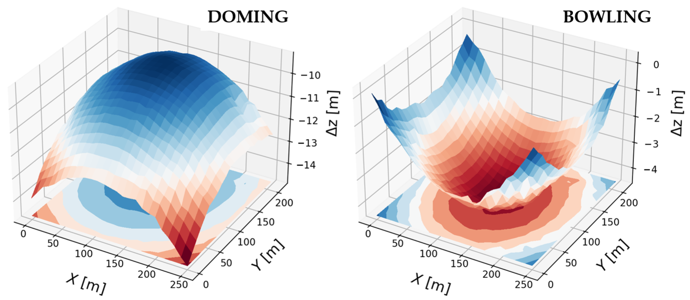
Funding

The project underlying this report was funded by the German Federal Ministry of Education and Research (German: Bundesministerium für Bildung und Forschung, BMBF) under the funding code 01BF2115C of the second Citizen Science funding guideline (2021–2024) (German: zweite Förderrichtlinie Citizen Science (2021–2024)). The responsibility for the content of this publication lies with the authors.

Data Availability Statement

The data presented in this study are available on request from the corresponding author. The data are not publicly available due to privacy reasons.

Acknowledgments

The authors would like to thank the Jena City Administration for the cooperation during the drone flight campaigns.

Conflicts of Interest

The authors declare no conflict of interest.

References

  1. Templin, T.; Popielarczyk, D. The Use of Low-Cost Unmanned Aerial Vehicles in the Process of Building Models for Cultural Tourism, 3D Web and Augmented/Mixed Reality Applications. Sensors 2020, 20, 5457. [Google Scholar] [CrossRef]
  2. Heipke, C. (Ed.) Photogrammetrie und Fernerkundung; Springer: Berlin/Heidelberg, Germany, 2017. [Google Scholar] [CrossRef]
  3. Eltner, A.; Hoffmeister, D.; Kaiser, A.; Karrasch, P.; Klingbeil, L.; Stöcker, C.; Rovere, A. (Eds.) UAVs for the Environmental Sciences: Methods and Applications; WBG Academic: Darmstadt, Germany, 2022. [Google Scholar]
  4. Sanz-Ablanedo, E.; Chandler, J.H.; Ballesteros-Pérez, P.; Rodríguez-Pérez, J.R. Reducing systematic dome errors in digital elevation models through better UAV flight design. Earth Surf. Process. Landforms 2020, 45, 2134–2147. [Google Scholar] [CrossRef]
  5. Kim, J.; Kim, S.; Ju, C.; Son, H.I. Unmanned Aerial Vehicles in Agriculture: A Review of Perspective of Platform, Control, and Applications. IEEE Access 2019, 7, 105100–105115. [Google Scholar] [CrossRef]
  6. Ju, C.; Son, H. Multiple UAV Systems for Agricultural Applications: Control, Implementation, and Evaluation. Electronics 2018, 7, 162. [Google Scholar] [CrossRef]
  7. Hassan-Esfahani, L.; Ebtehaj, A.M.; Torres-Rua, A.; McKee, M. Spatial Scale Gap Filling Using an Unmanned Aerial System: A Statistical Downscaling Method for Applications in Precision Agriculture. Sensors 2017, 17, 2106. [Google Scholar] [CrossRef]
  8. Christiansen, M.P.; Laursen, M.S.; Jørgensen, R.N.; Skovsen, S.; Gislum, R. Designing and Testing a UAV Mapping System for Agricultural Field Surveying. Sensors 2017, 17, 2703. [Google Scholar] [CrossRef]
  9. Wallace, L.O.; Lucieer, A.; Watson, C.S. Assessing the feasibility of uav-based lidar for high resolution forest change detection. Int. Arch. Photogramm. Remote Sens. Spat. Inf. Sci. 2012, XXXIX-B7, 499–504. [Google Scholar] [CrossRef]
  10. Schiefer, F.; Kattenborn, T.; Frick, A.; Frey, J.; Schall, P.; Koch, B.; Schmidtlein, S. Mapping forest tree species in high resolution UAV-based RGB-imagery by means of convolutional neural networks. ISPRS J. Photogramm. Remote Sens. 2020, 170, 205–215. [Google Scholar] [CrossRef]
  11. Shin, J.I.; Seo, W.W.; Kim, T.; Park, J.; Woo, C.S. Using UAV Multispectral Images for Classification of Forest Burn Severity—A Case Study of the 2019 Gangneung Forest Fire. Forests 2019, 10, 1025. [Google Scholar] [CrossRef]
  12. Mohan, M.; Leite, R.V.; Broadbent, E.N.; Wan Mohd Jaafar, W.S.; Srinivasan, S.; Bajaj, S.; Dalla Corte, A.P.; do Amaral, C.H.; Gopan, G.; Saad, S.N.M.; et al. Individual tree detection using UAV-lidar and UAV-SfM data: A tutorial for beginners. Open Geosci. 2021, 13, 1028–1039. [Google Scholar] [CrossRef]
  13. Thiel, C.; Mueller, M.M.; Epple, L.; Thau, C.; Hese, S.; Voltersen, M.; Henkel, A. UAS Imagery-Based Mapping of Coarse Wood Debris in a Natural Deciduous Forest in Central Germany (Hainich National Park). Remote Sens. 2020, 12, 3293. [Google Scholar] [CrossRef]
  14. Thiel, C.; Müller, M.M.; Berger, C.; Cremer, F.; Dubois, C.; Hese, S.; Baade, J.; Klan, F.; Pathe, C. Monitoring Selective Logging in a Pine-Dominated Forest in Central Germany with Repeated Drone Flights Utilizing A Low Cost RTK Quadcopter. Drones 2020, 4, 11. [Google Scholar] [CrossRef]
  15. Xu, Z.; Wu, L.; Shen, Y.; Li, F.; Wang, Q.; Wang, R. Tridimensional Reconstruction Applied to Cultural Heritage with the Use of Camera-Equipped UAV and Terrestrial Laser Scanner. Remote Sens. 2014, 6, 10413–10434. [Google Scholar] [CrossRef]
  16. Nex, F.; Remondino, F. UAV for 3D mapping applications: A review. Appl. Geomat. 2014, 6, 1–15. [Google Scholar] [CrossRef]
  17. Mukhamediev, R.I.; Symagulov, A.; Kuchin, Y.; Zaitseva, E.; Bekbotayeva, A.; Yakunin, K.; Assanov, I.; Levashenko, V.; Popova, Y.; Akzhalova, A.; et al. Review of Some Applications of Unmanned Aerial Vehicles Technology in the Resource-Rich Country. Appl. Sci. 2021, 11, 10171. [Google Scholar] [CrossRef]
  18. Erdelj, M.; Natalizio, E. UAV-assisted disaster management: Applications and open issues. In Proceedings of the 2016 International Conference on Computing, Networking and Communications (ICNC), Piscataway, NJ, USA, 5–8 June 2016; pp. 1–5. [Google Scholar] [CrossRef]
  19. Harwin, S.; Lucieer, A.; Osborn, J. The Impact of the Calibration Method on the Accuracy of Point Clouds Derived Using Unmanned Aerial Vehicle Multi-View Stereopsis. Remote Sens. 2015, 7, 11933–11953. [Google Scholar] [CrossRef]
  20. Yurtseven, H. Comparison of GNSS-, TLS- and Different Altitude UAV-Generated Datasets on The Basis of Spatial Differences. ISPRS Int. J.-Geo-Inf. 2019, 8, 175. [Google Scholar] [CrossRef]
  21. Eltner, A.; Schneider, D. Analysis of Different Methods for 3D Reconstruction of Natural Surfaces from Parallel-Axes UAV Images. Photogramm. Rec. 2015, 30, 279–299. [Google Scholar] [CrossRef]
  22. Clark, A.; Moorman, B.; Whalen, D.; Fraser, P. Arctic coastal erosion: UAV-SfM data collection strategies for planimetric and volumetric measurements. Arct. Sci. 2021, 7, 605–633. [Google Scholar] [CrossRef]
  23. Rosnell, T.; Honkavaara, E. Point cloud generation from aerial image data acquired by a quadrocopter type micro unmanned aerial vehicle and a digital still camera. Sensors 2012, 12, 453–480. [Google Scholar] [CrossRef] [PubMed]
  24. Nesbit, P.R.; Hubbard, S.M.; Hugenholtz, C.H. Direct Georeferencing UAV-SfM in High-Relief Topography: Accuracy Assessment and Alternative Ground Control Strategies along Steep Inaccessible Rock Slopes. Remote Sens. 2023, 14, 490. [Google Scholar] [CrossRef]
  25. James, M.R.; Robson, S.; d’Oleire Oltmanns, S.; Niethammer, U. Optimising UAV topographic surveys processed with structure-from-motion: Ground control quality, quantity and bundle adjustment. Geomorphology 2017, 280, 51–66. [Google Scholar] [CrossRef]
  26. Westoby, M.J.; Brasington, J.; Glasser, N.F.; Hambrey, M.J.; Reynolds, J.M. ‘Structure-from-Motion’ photogrammetry: A low-cost, effective tool for geoscience applications. Geomorphology 2012, 179, 300–314. [Google Scholar] [CrossRef]
  27. Hartley, R.; Zisserman, A. Multiple View Geometry in Computer Vision, 2nd ed.; Cambridge University Press: Cambridge, UK, 2003. [Google Scholar]
  28. Lowe, D.G. Distinctive Image Features from Scale-Invariant Keypoints. Int. J. Comput. Vis. 2004, 60, 91–110. [Google Scholar] [CrossRef]
  29. Zhuo, X.; Koch, T.; Kurz, F.; Fraundorfer, F.; Reinartz, P. Automatic UAV Image Geo-Registration by Matching UAV Images to Georeferenced Image Data. Remote Sens. 2017, 9, 376. [Google Scholar] [CrossRef]
  30. Smith, M.W.; Carrivick, J.L.; Quincey, D.J. Structure from motion photogrammetry in physical geography. Prog. Phys. Geogr. Earth Environ. 2016, 40, 247–275. [Google Scholar] [CrossRef]
  31. Deliry, S.I.; Avdan, U. Accuracy of Unmanned Aerial Systems Photogrammetry and Structure from Motion in Surveying and Mapping: A Review. J. Indian Soc. Remote Sens. 2021, 49, 1997–2017. [Google Scholar] [CrossRef]
  32. Javernick, L.; Brasington, J.; Caruso, B. Modeling the topography of shallow braided rivers using Structure-from-Motion photogrammetry. Geomorphology 2014, 213, 166–182. [Google Scholar] [CrossRef]
  33. Triggs, B.; McLauchlan, P.F.; Hartley, R.I.; Fitzgibbon, A.W. Bundle Adjustment—A Modern Synthesis. In Vision Algorithms: Theory and Practice; Triggs, B., Zisserman, A., Szeliski, R., Eds.; Springer: Berlin/Heidelberg, Germany, 2000; pp. 298–372. [Google Scholar]
  34. Carrivick, J.L.; Smith, M.W.; Quincey, D.J. Structure from Motion in the Geosciences; New Analytic Methods in Earth and Environmental Science; Wiley Blackwell: Chichester, UK, 2016. [Google Scholar]
  35. Eltner, A.; Kaiser, A.; Castillo, C.; Rock, G.; Neugirg, F.; Abellán, A. Image-based surface reconstruction in geomorphometry—Merits, limits and developments. Earth Surf. Dyn. 2016, 4, 359–389. [Google Scholar] [CrossRef]
  36. Sanz-Ablanedo, E.; Chandler, J.; Rodríguez-Pérez, J.; Ordóñez, C. Accuracy of Unmanned Aerial Vehicle (UAV) and SfM Photogrammetry Survey as a Function of the Number and Location of Ground Control Points Used. Remote Sens. 2018, 10, 1606. [Google Scholar] [CrossRef]
  37. James, M.R.; Robson, S. Mitigating systematic error in topographic models derived from UAV and ground-based image networks. Earth Surf. Process. Landforms 2014, 39, 1413–1420. [Google Scholar] [CrossRef]
  38. Magri, L.; Toldo, R. Bending the doming effect in structure from motion reconstructions through bundle adjustment. Int. Arch. Photogramm. Remote Sens. Spat. Inf. Sci. 2017, XLII-2/W6, 235–241. [Google Scholar] [CrossRef]
  39. Hastedt, H.; Luhmann, T.; Przybilla, H.J.; Rofallski, R. Evaluation of interior orientation modelling for cameras with aspheric lenses and image pre-processing with special emphasis to sfm reconstruction. Int. Arch. Photogramm. Remote Sens. Spat. Inf. Sci. 2021, XLIII-B2, 17–24. [Google Scholar] [CrossRef]
  40. Samboko, H.T.; Schurer, S.; Savenije, H.H.G.; Makurira, H.; Banda, K.; Winsemius, H. Evaluating low-cost topographic surveys for computations of conveyance. Geosci. Instrum. Methods Data Syst. 2022, 11, 1–23. [Google Scholar] [CrossRef]
  41. Griffiths, D.; Burningham, H. Comparison of pre- and self-calibrated camera calibration models for UAS-derived nadir imagery for a SfM application. Prog. Phys. Geogr. Earth Environ. 2019, 43, 215–235. [Google Scholar] [CrossRef]
  42. Carbonneau, P.E.; Dietrich, J.T. Cost-effective non-metric photogrammetry from consumer-grade sUAS: Implications for direct georeferencing of structure from motion photogrammetry. Earth Surf. Process. Landforms 2017, 42, 473–486. [Google Scholar] [CrossRef]
  43. Kaiser, S.; Boike, J.; Grosse, G.; Langer, M. The Potential of UAV Imagery for the Detection of Rapid Permafrost Degradation: Assessing the Impacts on Critical Arctic Infrastructure. Remote Sens. 2022, 14, 6107. [Google Scholar] [CrossRef]
  44. Wackrow, R.; Chandler, J.H. A convergent image configuration for DEM extraction that minimises the systematic effects caused by an inaccurate lens model. Photogramm. Rec. 2008, 23, 6–18. [Google Scholar] [CrossRef]
  45. Roncella, R.; Forlani, G. UAV Block Geometry Design and Camera Calibration: A Simulation Study. Sensors 2021, 21, 6090. [Google Scholar] [CrossRef]
  46. Vacca, G.; Dessì, A.; Sacco, A. The Use of Nadir and Oblique UAV Images for Building Knowledge. ISPRS Int. J. Geo-Inf. 2017, 6, 393. [Google Scholar] [CrossRef]
  47. Nesbit, P.R.; Hugenholtz, C.H. Enhancing UAV–SfM 3D Model Accuracy in High-Relief Landscapes by Incorporating Oblique Images. Remote Sens. 2019, 11, 239. [Google Scholar] [CrossRef]
  48. Zapico, I.; Molina, A.; Laronne, J.B.; Sánchez Castillo, L.; Martín Duque, J.F. Stabilization by geomorphic reclamation of a rotational landslide in an abandoned mine next to the Alto Tajo Natural Park. Eng. Geol. 2020, 264, 105321. [Google Scholar] [CrossRef]
  49. Štroner, M.; Urban, R.; Seidl, J.; Reindl, T.; Brouček, J. Photogrammetry Using UAV-Mounted GNSS RTK: Georeferencing Strategies without GCPs. Remote Sens. 2021, 13, 1336. [Google Scholar] [CrossRef]
  50. Stumpf, A.; Malet, J.P.; Allemand, P.; Pierrot-Deseilligny, M.; Skupinski, G. Ground-based multi-view photogrammetry for the monitoring of landslide deformation and erosion. Geomorphology 2015, 231, 130–145. [Google Scholar] [CrossRef]
  51. Bemis, S.P.; Micklethwaite, S.; Turner, D.; James, M.R.; Akciz, S.; Thiele, S.T.; Bangash, H.A. Ground-based and UAV-Based photogrammetry: A multi-scale, high-resolution mapping tool for structural geology and paleoseismology. J. Struct. Geol. 2014, 69, 163–178. [Google Scholar] [CrossRef]
  52. Carvajal-Ramírez, F.; Agüera-Vega, F.; Martínez-Carricondo, P.J. Effects of image orientation and ground control points distribution on unmanned aerial vehicle photogrammetry projects on a road cut slope. J. Appl. Remote Sens. 2016, 10, 034004. [Google Scholar] [CrossRef]
  53. TLUBN. Antares. Kartendienst des TLUBN. 2022. Available online: https://antares.thueringen.de/cadenza/;jsessionid=71996B707F06A05525B9B42337F8A6A1 (accessed on 15 July 2023).
  54. CLMS. Copernicus GMES Initial Operations/Copernicus Land Monitoring Services—Validation of Products (CORINE Land Cover Map 2018). 2021. Available online: https://land.copernicus.eu/pan-european/corine-land-cover/clc2018 (accessed on 15 July 2023).
  55. Gaveau, D.L.; Hill, R.A. Quantifying canopy height underestimation by laser pulse penetration in small-footprint airborne laser scanning data. Can. J. Remote Sens. 2003, 29, 650–657. [Google Scholar] [CrossRef]
  56. Hopkinson, C.; Chasmer, L.E.; Sass, G.; Creed, I.F.; Sitar, M.; Kalbfleisch, W.; Treitz, P. Vegetation class dependent errors in lidar ground elevation and canopy height estimates in a boreal wetland environment. Can. J. Remote Sens. 2005, 31, 191–206. [Google Scholar] [CrossRef]
  57. Litchi. 2023. Available online: https://flylitchi.com/ (accessed on 15 July 2023).
  58. DJI. DJI Mini 2 User Manual v1.4. 2022. Available online: https://dl.djicdn.com/downloads/DJI_Mini_2/20210630/DJI_Mini_2_User_Manual-EN.pdf (accessed on 15 July 2023).
  59. PPM. ppm 10xx GNSS Sensor. 2023. Available online: https://ppmgmbh.com/gps-produkte/externer-ppm-10xx-gnss-sensor/ (accessed on 15 July 2023).
  60. Novatel. VEXXIS® GNSS-500 Series Antennas. 2023. Available online: https://novatel.com/products/gps-gnss-antennas/vexxis-series-antennas/vexxis-gnss-500-series-antennas (accessed on 15 July 2023).
  61. Baboo, S.S.; Devi, M.R. An analysis of different resampling methods in Coimbatore, District. Glob. J. Comput. Sci. Technol. 2010, 5, 9611. [Google Scholar]
  62. Fritz, O.; Marx, S.; Herfort, B.; Kaiser, S.; Langer, M.; Lenz, J.; Thiel, C.; Zipf, A. Das Potenzial von Citizen Science für die Kartierung von Landschaftsveränderungen in arktischen Perma-frostregionen. AGIT—J. Fur Angew. Geoinformatik 2022, 8, 30–40. [Google Scholar] [CrossRef]
  63. Mueller, M.M.; Thiel, C.; Kaiser, S.; Lenz, J.; Langer, M.; Lantuit, H.; Marx, S.; Fritz, O.; Zipf, A. UndercoverEisAgenten—Monitoring Permafrost Thaw in the Arctic using Local Knowledge and UAVs. In Proceedings of the EGU General Assembly 2023, Vienna, Austria, 24–28 April 2023. EGU23-2698. [Google Scholar] [CrossRef]
  64. Goetz, J.; Brenning, A.; Marcer, M.; Bodin, X. Modeling the precision of structure-from-motion multi-view stereo digital elevation models from repeated close-range aerial surveys. Remote Sens. Environ. 2018, 210, 208–216. [Google Scholar] [CrossRef]
  65. Rogers, S.R.; Manning, I.; Livingstone, W. Comparing the spatial accuracy of digital surface models from four unoccupied aerial systems: Photogrammetry versus LiDAR. Remote Sens. 2020, 12, 2806. [Google Scholar] [CrossRef]
Figure 1. Examples of 3D model systematic deformations (bowling and doming) investigated in this study.
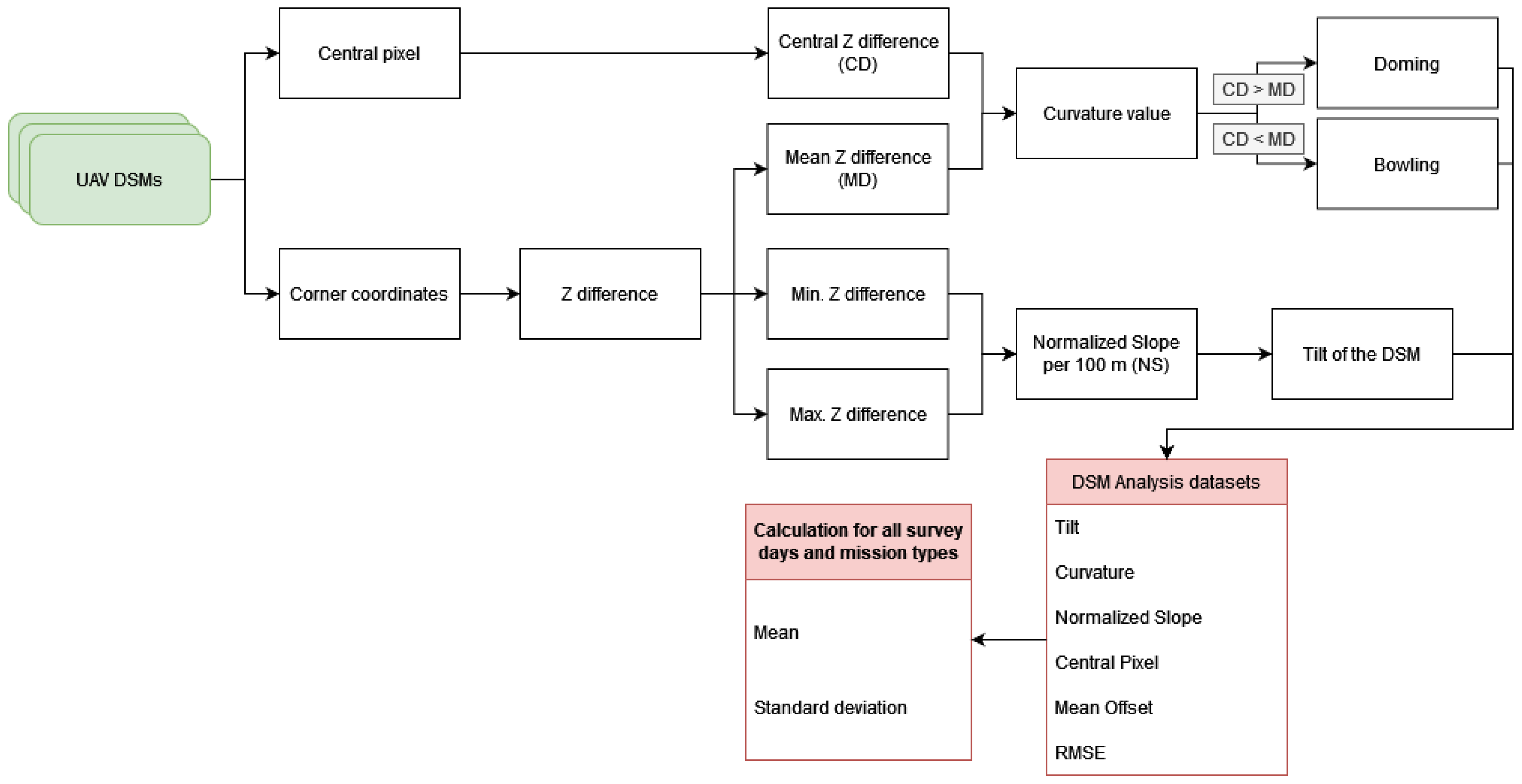
Remotesensing 15 04308 g001
Figure 2. Workflow of processing the SfM-MVS based HDMs. Green/yellow = input data, white = processing, red = output data. HDM = height difference model.
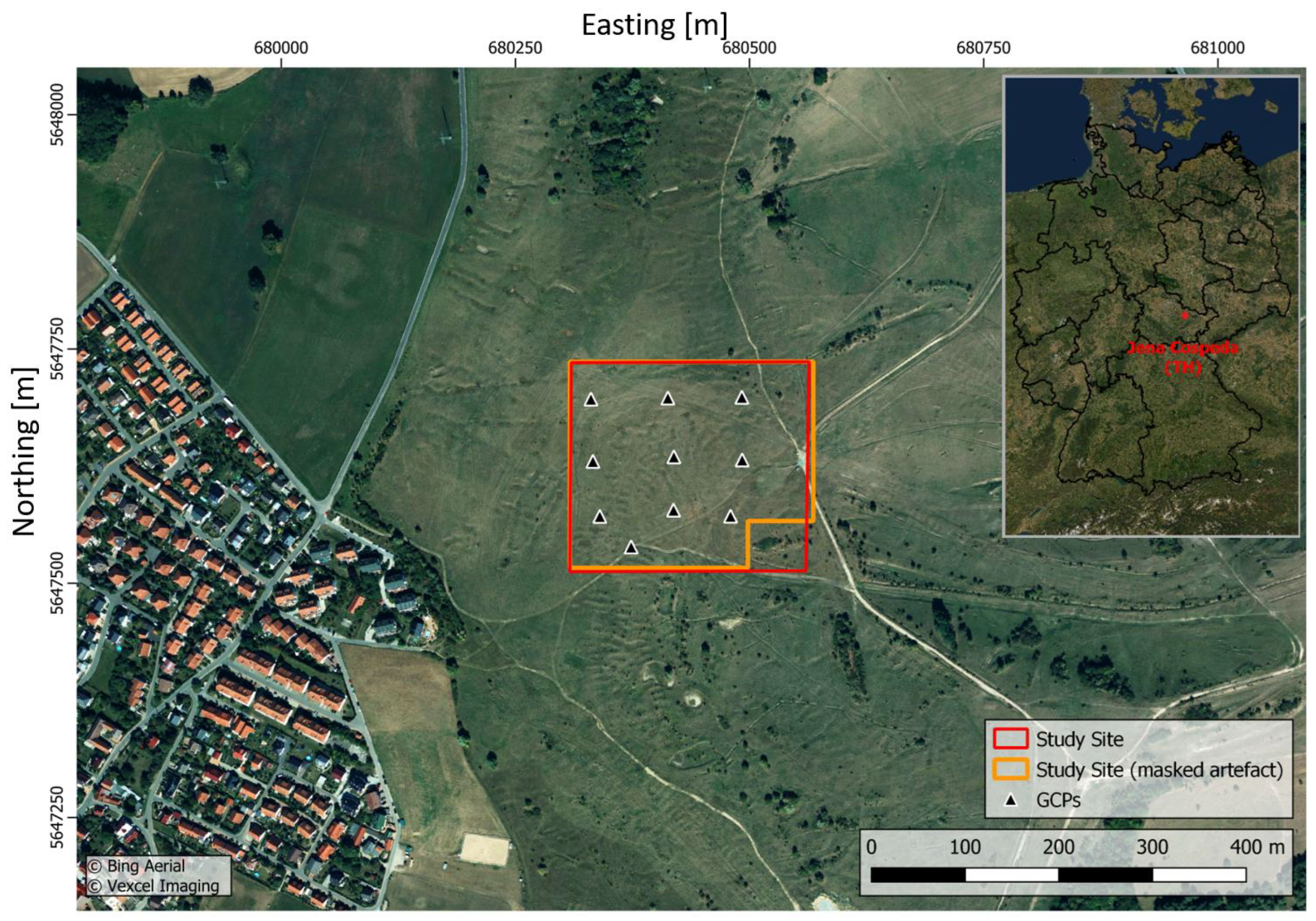
Remotesensing 15 04308 g002
Figure 3. Map of the study area (red) and masked study area (orange) with the locations of ten ground control points (black), all datasets are projected in WGS 84/UTM zone 32N. The Jena district of Cospeda is located in the western area. The city of Jena is located to the south of the study area.
Remotesensing 15 04308 g003
Figure 4. (A) Nadir and oblique view flight plan, the markers (purple) show individual waypoints on the UAV’s flight paths (yellow). The camera captures the image data with an angle of 0° (nadir flight pattern) and off-nadir angle of 30° (oblique view images). (B) POI flight plan, where the UAV circles the reference point (camera symbol in the center of the circular flight path) on the flight path. (C) Spiral flight plan where the UAV orbits the center reference point on the flight path in a spiral orbit. (D) Loop flight plan with three reference points (camera symbols), around which the UAV circles in an elliptical pattern. All figures are taken from the “Mission Hub” of the “Litchi” application.
Remotesensing 15 04308 g004
Figure 5. The extraction of curvature and slope deformation was performed by focusing on the central and edge pixels, leading to the computation of digital surface model (DSM) analysis products. These products were then employed to interpret the effects of deformation associated with various flight designs.
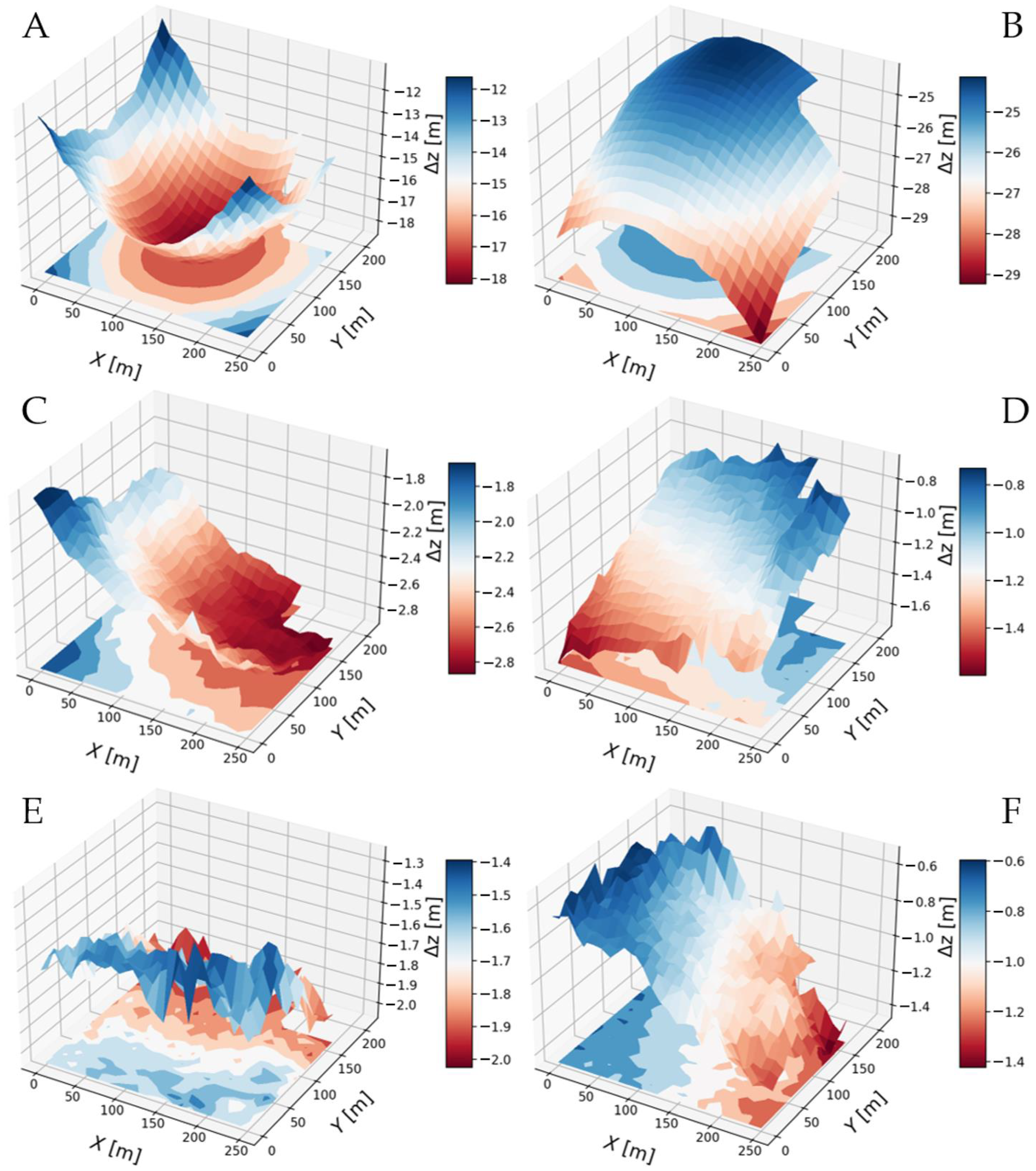
Remotesensing 15 04308 g005
Figure 6. 3D visualization of the different distortion effects observed in this study. Doming effect of the Nadir_120m flight mission on 19 May 2022 (A), bowling effect of the Nadir_120m flight mission on 10 May 2022 (B), slight doming effect of the Oblique_120m flight mission on 5 July 2022 (C). The other flight designs (POI_120m on 10 May 2022 (D), Spiral_120m on 10 May 2022 (E), Loop_120m on 18 May 2022 (F)) all show a varying degree of tilted distortions with no dominant tilt direction. It should be noted that the Δz-axis (z-offset) range is different for each subplot.
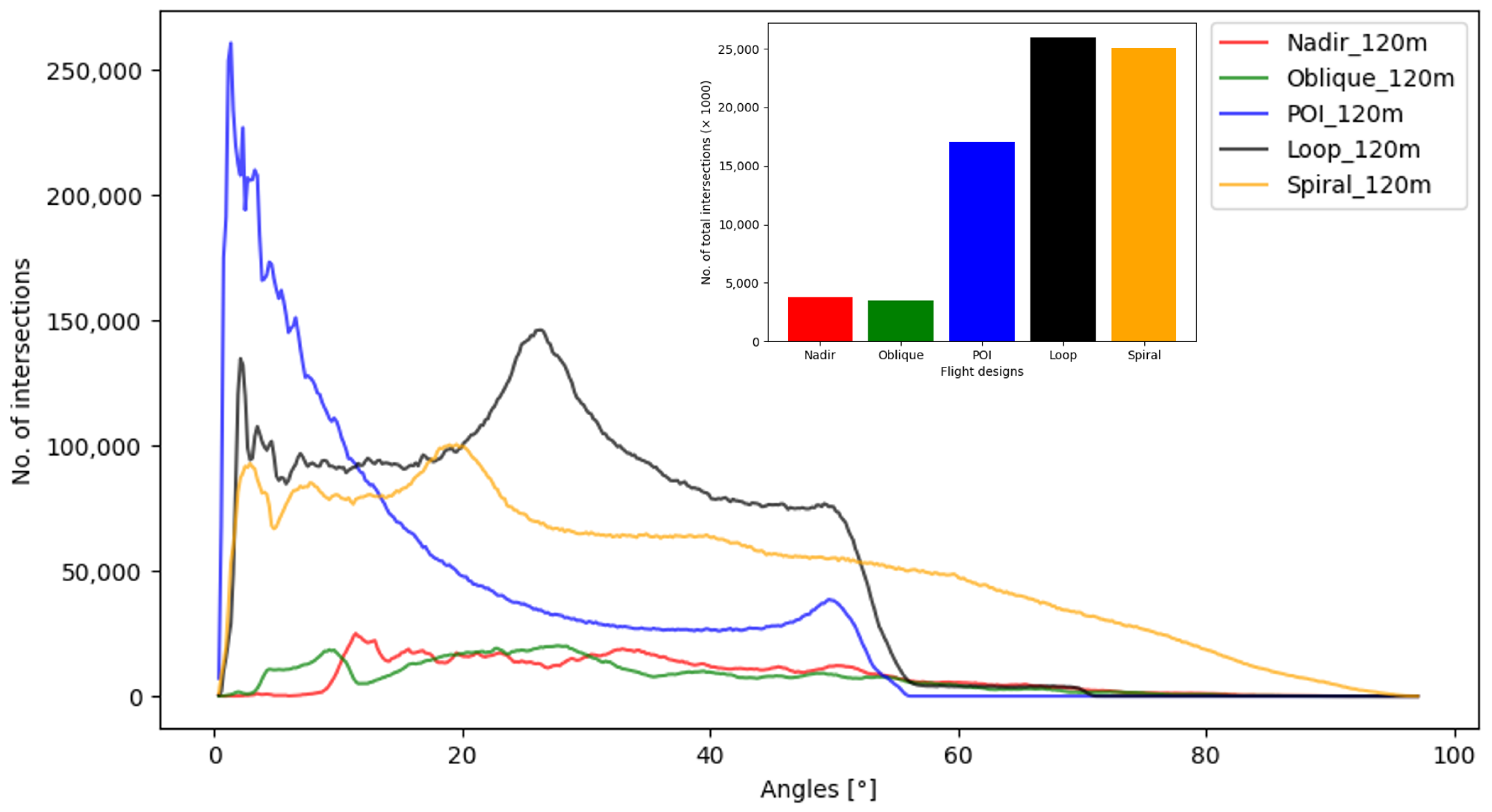
Remotesensing 15 04308 g006
Figure 7. Distribution of the angle intersections of the epipolar lines of all tie points for each mission design at 120 m flight altitude (POI: red, nadir: green, loops: blue, spirals: black, oblique: orange) and total number of intersections per mission design.
Remotesensing 15 04308 g007
Table 1. Overview of relevant scientific publications on the additional and exclusive use of oblique images to increase Z-accuracy. Additionally, different camera angles, heights, and image overlaps are examined.
Ref.HardwareGimbalAltitudeSiteAreaOverlap (%)Oblique Effect
[4]DJI Phantom 4 Pro (3×)Nadir, oblique, POI35–65 mUrban, flat2.1 ha65/45Doming sizes: nadir: 0.813 m, oblique: 0.149 m, POI: 0.101 m, nadir + ob: 0.082 m
[19]Canon 550DNadir, POI20–25 m (nadir), 18 m (POI)Nature, River3.5 ha80/90Significant improvement in horizontal and vertical accuracy
[22]DJI M210, senseFly eBee X, DJI Mavic ProNadir, oblique80–100 mPermafrost0.3–0.5 ha70/80Increases z-accuracy significantly (MAE from 0.2 m (nadir) to 0.03 m (nadir + oblique))
[24]DJI Phantom 4 RTKNadir, oblique30–60 mHilly, steep ravinesn.a.n.a.Nadir significantly higher standard deviation and mean error than oblique images or combination of nadir and oblique images
[37]Canon 450DNadir, obliqueVaryingVolcanic rock samplen.a.n.a.Reduce the doming effect by up to two orders of magnitude
[45]DJI Phantom 3 ProNadir, oblique, POI49 mFlat, hilly27.4 ha80/70Improved accuracy by 5 to 9 orders of magnitude
[46]FlyNovexNadir, oblique90 m (nadir), 50 m (oblique)Urbann.a.80/75 (nadir), 80/80 (oblique)50–90% improvement in accuracy
[47]DJI Phantom 3 ProNadir, oblique40 mHilly0.7 ha90/90, 90/70, 70/70Accuracies of oblique images in the range 20–35° higher than oblique images 0–15°
[48]DJI Phantom 4 ProNadir, oblique65 mPlateau, steep ravinesn.a.80/80Error reduction up to 50%
[49]DJI Phantom 4 RTKNadir, oblique100 m (nadir), 75/125 m (oblique)Fallow land, ruraln.a.75/75Combination nadir + oblique with best results, higher oblique angles with better results
Table 2. UAV specifications of DJI Mini 2 [58].
UAVDJI Mini 2
GNSSGPS/GLONASS/Galileo
Image sensorDJI FC7303; 1/2,3″-CMOS; Focal length 24 mm (35 mm equivalent)
No. of pixels4000 × 3000 (12 MP)
Focal length4.49 mm
Field of view73° (horizontal); 53° (vertical); 84° (diagonal)
Electronic shutter4–1/8000 s
Data formatDNG (16 bit)
Aircraft weight249 g
Table 3. UAV missions and acquisition parameters for both 120 m and 80 m altitudes. All values are averaged for the five survey dates. The camera acquisition parameters were set to “auto” to balance any brightness differences between images. The covered area refers to the entire area covered by the UAV acquisitions. The area of interest (see Figure 3), is a subset of the UAV coverage area.
Missions (120 m)
ParameterNadirObliquePOISpiralLoop
Avg. number of images9390123161128
Avg. flight time (min)1414697
Gimbal angle (°)030500–5017–43
Max. geometric resolution (cm)4.124.936.945.464.75
Overlap (front/side) (%)80/8080/80NANANA
Flight speed (m/s)3.33.33.33.33.3
Missions (80 m)
ParameterNadirObliquePOISpiralLoop
Avg. number of images182183123159127
Avg. flight time (min)1919697
Gimbal angle (°)030610–6126–54
Max. geometric resolution (cm)2.83.355.274.33.64
Overlap (front/side) (%)80/8080/80NANANA
Flight speed (m/s)3.33.33.33.33.3
Table 4. Summary of the UAV processing parameters (Agisoft Metashape v1.8.3) used for the processing of all datasets. f, focal length; cx and cy, principal point offset; k1, k2, and k3, radial distortion coefficients; p1 and p2, tangential distortion coefficients.
Processing ParametersParameter Values
Photo alignment accuracyHigh
Image preselectionGeneric/Source
Key point limit40,000
Tie point limit4000
Guided image matchingNo
Adaptive camera model fittingNo
Camera positional accuracy10 m
Adapted camera parametersf, cx, cy, k1–k3, p1, p2
Dense cloud qualityHigh
Depth filteringOff
Table 5. Concise explanation of parameters from UAV data processing results.
ParameterExplanation
No. of tie pointsThe total number of valid matching points between different images.
Reprojection error (pix)The root mean square error between the reconstructed 3D point and its original 2D projection on the image. Measured in pixels.
No. of points (dense cloud)The total number of 3D points generated in the dense point cloud during processing.
fThe estimated focal length of the camera measured in pixels.
cx, cyThe estimated coordinates of the principal point, which is where the optical axis of the lens intersects the image plane.
k1, k2, k3The estimated coefficients for radial distortion correction.
p1, p2The estimated coefficients for tangential distortion correction.
Average error in camera pos. (X, Y, Z) (m)The average error in determining the camera’s position in X-, Y-, and Z-directions.
RMSE of check points (X, Y, Z) (m)The root mean square error of the positions of check points, which are pre-known reference points, in X-, Y-, and Z-directions.
Projections per image/per tie pointSignifies average tie point projections per image and per tie point, influencing 3D reconstruction accuracy in SfM workflows.
Intersections per image/per tie pointQuantifies image overlaps and their distribution per image and per tie point, crucial for accurate 3D point positioning. Optimal intersecting angles enhance reconstruction stability and accuracy.
Table 6. Comparison of estimated camera model parameters for mission designs at different flight altitudes (80 m vs. 120 m), averaged over five repetitions. The parameters include the estimated focal length (f), principal point offsets (cx, cy), radial distortion coefficients (k1, k2, k3), and tangential distortion coefficients (p1, p2).
Parameter (Avg. 5 Repeats)NadirObliquePOISpiralLoop
120 m Flight Altitude
f2731.812911.552945.832938.702927.75
cx, cy6.36, −9.083.08, −8.820.49, −12.792.48, −5.123.60, −5.23
k1, k2, k30.17, −0.43, 0.270.17, −0.51, 0.360.11, −0.35, 0.220.11, −0.34, 0.210.14, −0.38, 0.30
p1, p22.2 ×  10 4 , 9.0 ×  10 4 −7.0 ×  10 5 , −5.0 ×  10 4 −1.8 ×  10 4 , 6.7 ×  10 4 −3.1 ×  10 4 , 3.4 ×  10 4 −3.2 ×  10 4 , 4.1 ×  10 4
80 m Flight Altitude
f2823.922911.452941.062933.992933.29
cx, cy5.10, −10.281.22, −8.970.35, −11.713.54, −5.413.32, −6.49
k1, k2, k30.17, −0.49, 0.330.17, −0.27, 0.370.11, −0.36, 0.230.12, −0.39, 0.260.13, −0.42, 0.28
p1, p22.0 ×  10 4 , 7.8 ×  10 4 −3.8 ×  10 5 , −5.5 ×  10 5 −1.7 ×  10 4 , 6.7 ×  10 4 −2.3 ×  10 4 , 3.8 ×  10 4 −3.7 ×  10 4 , 3.6 ×  10 4
Table 7. UAV data processing results, estimated camera model parameters averaged for each mission design based on five repetitions and check point accuracies. The camera parameters were estimated for each dataset independently.
Mission DesignNadirObliquePOISpiralLoop
120 m Flight Altitude
No. of tie points1.5 ×  10 4 2.5 ×  10 4 1.8 ×  10 4 1.7 ×  10 4 1.9 ×  10 4
Reprojection error (pix)1.071.190.680.650.82
No. of points (dense cloud)2.0 ×  10 7 2.6 ×  10 7 2.1 ×  10 7 2.3 ×  10 7 1.8 ×  10 7
Average error in camera pos. (X, Y, Z) (m)0.96, 1.25, 1.220.95, 0.65, 0.630.23, 0.28, 0.260.56, 0.74, 0.840.54, 0.67, 0.74
RMSE of check points (X, Y, Z) (m)4.26, 3.71, 19.651.43, 1.91, 2.031.20, 2.02, 1.441.40, 2.38, 2.511.38, 1.52, 2.02
No. of projections1.4 ×  10 5 1.8 ×  10 5 3.1 ×  10 5 3.0 ×  10 5 3.5 ×  10 5
per image/per tie point1.5 ×  10 3 /92.0 ×  10 3 /72.5 ×  10 3 /171.9 ×  10 3 /172.7 ×  10 3 /18
No. of intersections9.5 ×  10 5 8.7 ×  10 5 4.3 ×  10 6 6.3 ×  10 6 6.5 ×  10 6
per image/per tie point1.0 ×  10 4 /679.7 ×  10 3 /323.4 ×  10 4 /2413.9 ×  10 4 /3525.1 ×  10 4 /334
80 m Flight Altitude
No. of tie points 3.9 × 10 4 5.1 × 10 4 3.0 × 10 4 3.5 × 10 4 3.2 × 10 4
Reprojection error (pix)1.101.160.680.830.85
No. of points (dense cloud) 3.4 × 10 7 3.9 × 10 7 1.5 × 10 7 2.2 × 10 7 2.6 × 10 7
Average error in camera pos. (X, Y, Z) (m)0.45, 0.48, 1.130.57, 0.47, 0.550.22, 0.27, 0.260.20, 0.24, 0.480.20, 0.23, 0.30
RMSE of check points (X, Y, Z) (m)2.32, 1.62, 6.500.91, 0.41, 0.950.90, 1.89, 1.510.81, 1.73, 1.160.69, 1.13, 0.65
No. of projections 4.4 × 10 5 4.5 × 10 5 3.8 × 10 5 4.0 × 10 5 3.6 × 10 5
per image/per tie point 2.5 × 10 3 /11 2.4 × 10 3 /9 3.0 × 10 3 /13 2.5 × 10 3 /11 2.8 × 10 3 /11
No. of intersections 3.5 × 10 6 3.1 × 10 6 3.3 × 10 6 4.2 × 10 6 3.6 × 10 6
per image/per tie point 2.0 × 10 4 /93 1.7 × 10 4 /60 2.6 × 10 4 /112 2.6 × 10 4 /123 2.8 × 10 4 /113
Table 8. Overview of computed DSM analysis data derived from masked height difference models. “Offset CenterPixel” refers to the Z-value deviation of the HDM center pixel from the reference DTM (m), “Offset EdgePixels” denotes the mean Z-value deviation of the four HDM corner pixels from the reference DTM (m), “curvature” quantifies the degree of DSM deformation (m), “normalized slope” signifies the normalized elevation difference per 100 m (m), “mean offset” represents the mean offset between all UAV DSM and lidar DSM pixels (m), and “mean slope” is the average slope of the height difference model (°). For all parameters, an ideal value is zero, indicating no deviation. In the color coding, red corresponds to high negative deviation and blue to high positive deviation.
DateFilenameOffset CenterPixelOffset EdgePixelsCurvatureNormalized SlopeMean OffsetMean Slope
10 May 2022Nadir_120m−14.79−17.672.88−1.24−15.721.31
18 May 2022Nadir_120m−11.06−13.13−1.93−1.31−18.093.08
19 May 2022Nadir_120m−18.2−11.16−1.04−1.12−15.572.75
28 Jun 2022Nadir_120m−1.9−1.58−1.32−1.11−1.310.64
5 July 2022Nadir_120m−1.07−1.45−1.62−1.15−1.091.03
10 May 2022Nadir_80m−1.88−13.323.44−1.98−11.061.42
18 May 2022Nadir_80m−1.47−1.09−1.38−1.22−1.132.47
19 May 2022Nadir_80m−10.08−1.38−1.7−1.23−1.292.95
28 Jun 2022Nadir_80m−1.05−1.49−1.56−1.39−1.50.62
5 July 2022Nadir_80m−1.44−1.19−1.25−1.26−1.891.64
10 May 2022Oblique_120m−1.52−1.530.01−1.43−1.430.49
18 May 2022Oblique_120m−1.67−1.34−1.33−1.26−1.470.36
19 May 2022Oblique_120m−1.3−1.04−1.26−1.28−1.140.29
28 Jun 2022Oblique_120m−1.52−1.36−1.16−1.53−1.340.57
5 July 2022Oblique_120m−1.69−1.03−1.66−1.27−1.480.33
10 May 2022Oblique_80m−1.74−1.66−1.08−1.4−1.620.37
18 May 2022Oblique_80m−1.65−1.08−1.57−1.24−1.370.35
19 May 2022Oblique_80m−1.98−1.44−1.54−1.12−1.70.35
28 Jun 2022Oblique_80m−1.63−1.81−1.82−1.41−1.360.38
5 July 2022Oblique_80m−1.23−1.26−1.97−1.59−1.930.45
10 May 2022POI_120m−1.1−1.320.22−1.31−1.110.25
18 May 2022POI_120m−1.97−10.03−1.22−1.030.27
19 May 2022POI_120m−1.81−1.920.11−1.19−1.870.27
28 Jun 2022POI_120m−1.45−1.760.31−1.28−1.510.41
5 July 20225POI_120m−1.43−1.710.28−1.07−1.540.26
10 May 2022POI_80m−1.12−1.340.22−1.19−1.140.21
18 May 2022POI_80m−1.82−1.870.05−1.03−1.830.24
19 May 2022POI_80m−1.28−1.310.03−1.29−1.290.34
28 Jun 2022POI_80m−1.34−1.640.3−1.15−1.420.33
5 July 2022POI_80m−1.2−1.450.25−1.04−1.290.27
10 May 2022Loop_120m−1.01−1.95−1.06−1.07−1.960.2
18 May 2022Loop_120m−1.05−1.87−1.18−1.22−1.990.29
19 May 2022Loop_120m−1.07−1.84−1.23−1.24−10.32
28 Jun 2022Loop_120m−1.85−1.940.09−1.1−1.820.32
5 July 2022Loop_120m−1.27−1.420.15−1.17−1.30.26
10 May 2022Loop_80m−1.82−1.930.11−1.25−1.820.23
18 May 2022Loop_80m−1.88−1.920.04−1.1−1.860.22
19 May 2022Loop_80m−1.81−1.61−1.2−1.24−1.740.34
28 Jun 2022Loop_80m−1.62−1.940.32−1.33−1.660.31
5 July 2022Loop_80m−1.87−1.170.3−1.31−1.910.32
10 May 2022Spiral_120m−1.8−1.77−1.03−1.2−1.740.3
18 May 2022Spiral_120m−1.65−1.58−1.07−1.16−1.660.36
19 May 2022Spiral_120m−1.91−1.9−1.01−1.17−1.940.27
28 Jun 2022Spiral_120m−1.32−1.610.29−1.18−1.40.33
5 July 2022Spiral_120m−1−1.090.09−1.19−1.080.24
10 May 2022Spiral_80m−1.33−1.28−1.05−1.32−1.310.27
18 May 2022Spiral_80m−1.34−1.3−1.04−1.16−1.330.29
19 May 2022Spiral_80m−1.05−1.01−1.04−1.16−1.040.29
28 Jun 2022Spiral_80m−1.74−1.950.21−1.37−1.80.36
5 July 2022Spiral_80m−1.1−1.360.26−1.15−1.210.31
Disclaimer/Publisher’s Note: The statements, opinions and data contained in all publications are solely those of the individual author(s) and contributor(s) and not of MDPI and/or the editor(s). MDPI and/or the editor(s) disclaim responsibility for any injury to people or property resulting from any ideas, methods, instructions or products referred to in the content.

