A Data-Driven Approach for Urban Heat Island Predictions: Rethinking the Evaluation Metrics and Data Preprocessing


Abstract
1. Introduction
2. Methodology
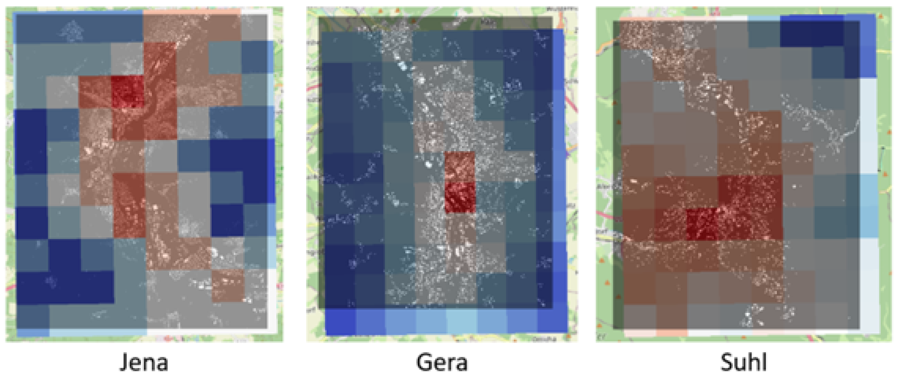
2.1. Study Area
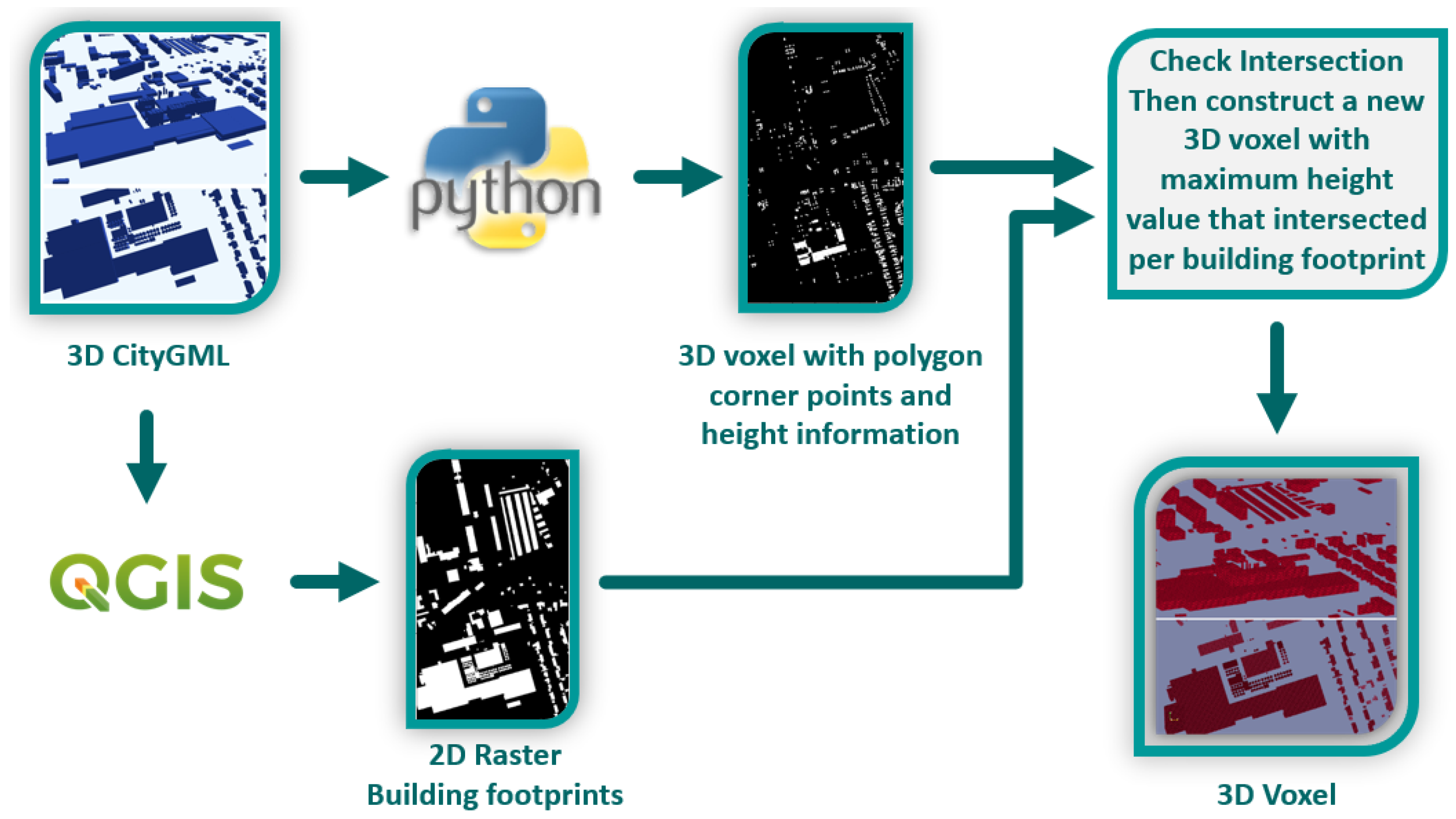
2.2. Creating 2D Building Volume Data in Raster
2.2.1. Retrieving 2D Building Footprint Areas
2.2.2. Real-World Coordinate System to Voxel Coordinate System
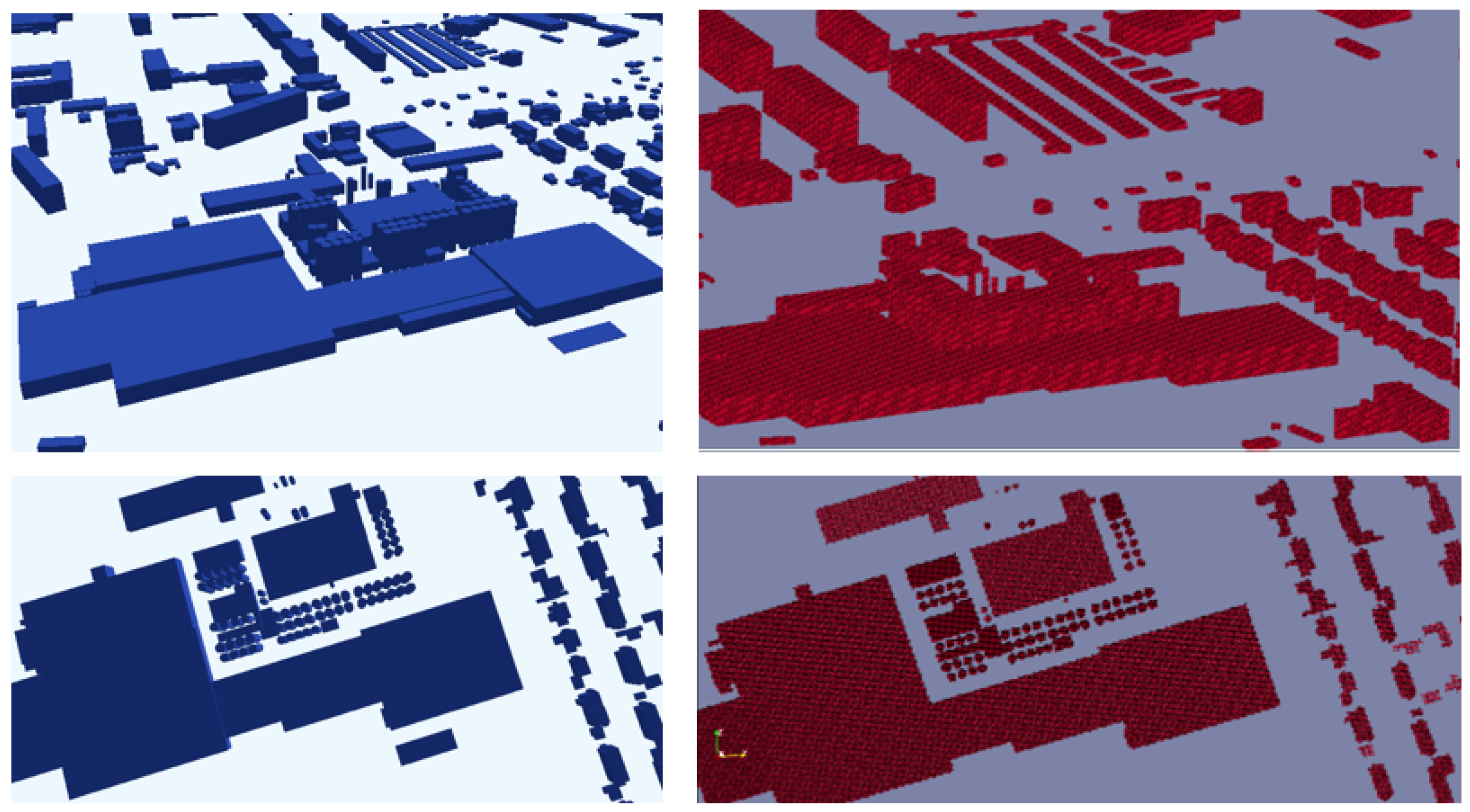
2.2.3. Assigning the Height Information to Building Footprints
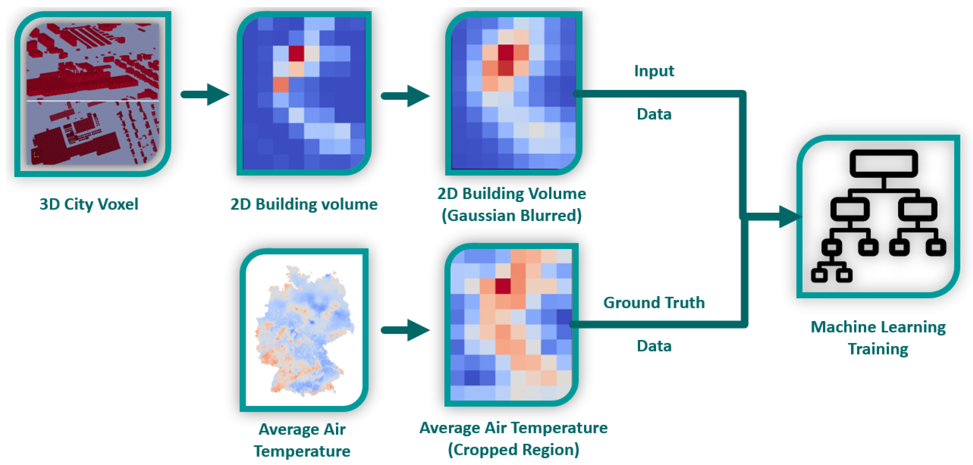
2.3. Machine Learning Training
3. Results
4. Discussion
5. Conclusions
Author Contributions
Funding
Data Availability Statement
Acknowledgments
Conflicts of Interest
References
- Han, Y.; Taylor, J.E.; Pisello, A.L. Toward mitigating urban heat island effects: Investigating the thermal-energy impact of bio-inspired retro-reflective building envelopes in dense urban settings. Energy Build. 2015, 102, 380–389. [Google Scholar] [CrossRef]
- Lan, Y.; Zhan, Q. How do urban buildings impact summer air temperature? The effects of building configurations in space and time. Build. Environ. 2017, 125, 88–98. [Google Scholar] [CrossRef]
- Liu, L.; Liu, J.; Jin, L.; Liu, L.; Gao, Y.; Pan, X. Climate-conscious spatial morphology optimization strategy using a method combining local climate zone parameterization concept and urban canopy layer model. Build. Environ. 2020, 185, 107301. [Google Scholar] [CrossRef]
- Ren, Z.; Jiang, B.; Seipel, S. Capturing and characterizing human activities using building locations in America. ISPRS Int. J. Geo-Inf. 2019, 8, 200. [Google Scholar] [CrossRef]
- Zhong, C.; Schläpfer, M.; Müller Arisona, S.; Batty, M.; Ratti, C.; Schmitt, G. Revealing centrality in the spatial structure of cities from human activity patterns. Urban Stud. 2017, 54, 437–455. [Google Scholar] [CrossRef]
- Tehrani, A.A.; Veisi, O.; Delavar, Y.; Bahrami, S.; Sobhaninia, S.; Mehan, A. Predicting urban Heat Island in European cities: A comparative study of GRU, DNN, and ANN models using urban morphological variables. Urban Clim. 2024, 56, 102061. [Google Scholar] [CrossRef]
- Arnfield, A.J. Two decades of urban climate research: A review of turbulence, exchanges of energy and water, and the urban heat island. Int. J. Climatol. J. R. Meteorol. Soc. 2003, 23, 1–26. [Google Scholar] [CrossRef]
- Yang, Z.; Chen, Y.; Zheng, Z.; Huang, Q.; Wu, Z. Application of building geometry indexes to assess the correlation between buildings and air temperature. Build. Environ. 2020, 167, 106477. [Google Scholar] [CrossRef]
- Eliasson, I. The use of climate knowledge in urban planning. Landsc. Urban Plan. 2000, 48, 31–44. [Google Scholar] [CrossRef]
- Ng, E. Towards planning and practical understanding of the need for meteorological and climatic information in the design of high-density cities: A case-based study of Hong Kong. Int. J. Climatol. 2012, 32, 582–598. [Google Scholar] [CrossRef]
- Fathi, S.; Srinivasan, R.; Fenner, A.; Fathi, S. Machine learning applications in urban building energy performance forecasting: A systematic review. Renew. Sustain. Energy Rev. 2020, 133, 110287. [Google Scholar] [CrossRef]
- Liu, L.; Silva, E.A.; Wu, C.; Wang, H. A machine learning-based method for the large-scale evaluation of the qualities of the urban environment. Comput. Environ. Urban Syst. 2017, 65, 113–125. [Google Scholar] [CrossRef]
- Tekouabou, S.C.K.; Diop, E.B.; Azmi, R.; Jaligot, R.; Chenal, J. Reviewing the application of machine learning methods to model urban form indicators in planning decision support systems: Potential, issues and challenges. J. King Saud-Univ.-Comput. Inf. Sci. 2022, 34, 5943–5967. [Google Scholar] [CrossRef]
- Venter, Z.S.; Brousse, O.; Esau, I.; Meier, F. Hyperlocal mapping of urban air temperature using remote sensing and crowdsourced weather data. Remote Sens. Environ. 2020, 242, 111791. [Google Scholar] [CrossRef]
- Yoo, S.J.; Kwon, T.; Lyoo, Y.S. Challenges of influenza A viruses in humans and animals and current animal vaccines as an effective control measure. Clin. Exp. Vaccine Res. 2018, 7, 1–15. [Google Scholar] [CrossRef] [PubMed]
- Fan, C.; Zou, B.; Li, J.; Wang, M.; Liao, Y.; Zhou, X. Exploring the relationship between air temperature and urban morphology factors using machine learning under local climate zones. Case Stud. Therm. Eng. 2024, 55, 104151. [Google Scholar] [CrossRef]
- Lau, T.K.; Lin, T.P. Investigating the relationship between air temperature and the intensity of urban development using on-site measurement, satellite imagery and machine learning. Sustain. Cities Soc. 2024, 100, 104982. [Google Scholar] [CrossRef]
- Zheng, Z.; Zhou, W.; Yan, J.; Qian, Y.; Wang, J.; Li, W. The higher, the cooler? Effects of building height on land surface temperatures in residential areas of Beijing. Phys. Chem. Earth Parts A/B/C 2019, 110, 149–156. [Google Scholar] [CrossRef]
- Hu, Y.; Dai, Z.; Guldmann, J.M. Modeling the impact of 2D/3D urban indicators on the urban heat island over different seasons: A boosted regression tree approach. J. Environ. Manag. 2020, 266, 110424. [Google Scholar] [CrossRef]
- Li, H.; Li, Y.; Wang, T.; Wang, Z.; Gao, M.; Shen, H. Quantifying 3D building form effects on urban land surface temperature and modeling seasonal correlation patterns. Build. Environ. 2021, 204, 108132. [Google Scholar] [CrossRef]
- Oke, T.R. The heat island of the urban boundary layer: Characteristics, causes and effects. In Wind Climate in Cities; Springer: Dordrecht, The Netherlands, 1995; pp. 81–107. [Google Scholar]
- Stewart, I.D.; Oke, T.R. Local climate zones for urban temperature studies. Bull. Am. Meteorol. Soc. 2012, 93, 1879–1900. [Google Scholar] [CrossRef]
- Voogt, J.A.; Oke, T.R. Thermal remote sensing of urban climates. Remote Sens. Environ. 2003, 86, 370–384. [Google Scholar] [CrossRef]
- Wu, J. Urban sustainability: An inevitable goal of landscape research. Landsc. Ecol. 2010, 25, 1–4. [Google Scholar] [CrossRef]
- Zhou, W.; Huang, G.; Cadenasso, M.L. Does spatial configuration matter? Understanding the effects of land cover pattern on land surface temperature in urban landscapes. Landsc. Urban Plan. 2011, 102, 54–63. [Google Scholar] [CrossRef]
- Lin, A.; Wu, H.; Luo, W.; Fan, K.; Liu, H. How does urban heat island differ across urban functional zones? Insights from 2D/3D urban morphology using geospatial big data. Urban Clim. 2024, 53, 101787. [Google Scholar] [CrossRef]
- Liu, B.; Guo, X.; Jiang, J. How urban morphology relates to the urban heat island effect: A multi-indicator study. Sustainability 2023, 15, 10787. [Google Scholar] [CrossRef]
- Raaymakers, T. Understanding Urban Temperature Differences through 2D/3D Urban Morphology. In Context of the Belt & Road Initiative; Wageningen University and Research: Wageningen, The Netherlands, 2024. [Google Scholar]
- Isa, N.A.; Salleh, S.A.; Mohd, W.M.N.W.; Chan, A.; Ooi, M.C.G.; Zakaria, N.H.; Islam, M.A. Building Volume Effects on Ambient Temperature In The Kuala Lumpur City. In IOP Conference Series: Earth and Environmental Science, Proceedings of the 15th International Conference on Atmospheric Sciences and Applications to Air Quality, Kuala Lumpur, Malaysia, 28–30 October 2019; IOP Publishing: Bristol, UK, 2020; Volume 489, p. 012011. [Google Scholar]
- Wang, Z.; Bovik, A.C.; Sheikh, H.R.; Simoncelli, E.P. Image quality assessment: From error visibility to structural similarity. IEEE Trans. Image Process. 2004, 13, 600–612. [Google Scholar] [CrossRef]
- Zhang, R.; Isola, P.; Efros, A.A.; Shechtman, E.; Wang, O. The unreasonable effectiveness of deep features as a perceptual metric. In Proceedings of the IEEE Conference on Computer Vision and Pattern Recognition, Salt Lake City, UT, USA, 18–23 June 2018; pp. 586–595. [Google Scholar]
- Ghildyal, A.; Liu, F. Attacking perceptual similarity metrics. arXiv 2023, arXiv:2305.08840. [Google Scholar]
- Tancik, M.; Weber, E.; Ng, E.; Li, R.; Yi, B.; Wang, T.; Kristoffersen, A.; Austin, J.; Salahi, K.; Ahuja, A.; et al. Nerfstudio: A modular framework for neural radiance field development. In Proceedings of the ACM SIGGRAPH 2023 Conference Proceedings, Los Angeles, CA, USA, 6–10 August 2023; pp. 1–12. [Google Scholar]
- Voogt, J.A.; Oke, T. Effects of urban surface geometry on remotely-sensed surface temperature. Int. J. Remote. Sens. 1998, 19, 895–920. [Google Scholar] [CrossRef]
- Cai, Z.; Han, G.; Chen, M. Do water bodies play an important role in the relationship between urban form and land surface temperature? Sustain. Cities Soc. 2018, 39, 487–498. [Google Scholar] [CrossRef]
- Guo, G.; Zhou, X.; Wu, Z.; Xiao, R.; Chen, Y. Characterizing the impact of urban morphology heterogeneity on land surface temperature in Guangzhou, China. Environ. Model. Softw. 2016, 84, 427–439. [Google Scholar] [CrossRef]
- Wu, C.D.; Lung, S.C.C.; Jan, J.F. Development of a 3-D urbanization index using digital terrain models for surface urban heat island effects. ISPRS J. Photogramm. Remote Sens. 2013, 81, 1–11. [Google Scholar] [CrossRef]
- Ren, C.; Cai, M.; Li, X.; Shi, Y.; See, L. Developing a rapid method for 3-dimensional urban morphology extraction using open-source data. Sustain. Cities Soc. 2020, 53, 101962. [Google Scholar] [CrossRef]
- Heeramaglore, M.; Kolbe, T.H. Semantically enriched voxels as a common representation for comparison and evaluation of 3D building models. ISPRS Ann. Photogramm. Remote Sens. Spat. Inf. Sci. 2022, 10, 89–96. [Google Scholar] [CrossRef]
- Padsala, R.; Gebetsroither-Geringer, E.; Bao, K.; Coors, V. The Application of CityGML Food Water Energy ADE to Estimate the Biomass Potential for a Land Use Scenario. In CITIES 20.50–Creating Habitats for the 3rd Millennium: Smart–Sustainable–Climate Neutral, Proceedings of the REAL CORP 2021, 26th International Conference on Urban Development, Regional Planning and Information Society, Vienna, Austria, 7–10 September 2021; CORP—Competence Center of Urban and Regional Planning: Vienna, Austria, 2021; pp. 851–861. [Google Scholar]
- Biljecki, F.; Ledoux, H.; Stoter, J. An improved LOD specification for 3D building models. Comput. Environ. Urban Syst. 2016, 29, 25–37. [Google Scholar] [CrossRef]
- Henn, A.; Römer, C.; Gröger, G.; Plümer, L. Automatic classification of building types in 3D city models: Using SVMs for semantic enrichment of low resolution building data. GeoInformatica 2012, 16, 281–306. [Google Scholar] [CrossRef]
- Hofierka, J.; Zlocha, M. A new 3-D solar radiation model for 3-D city models. Trans. GIS 2012, 16, 681–690. [Google Scholar] [CrossRef]
- Mulder, D. Automatic Repair of 3D City Building Model Using a Voxel–Based Repair Method. Master Thesis, Delft University of Technology, Delft, The Netherlands, 2015. [Google Scholar]
- Nourian, P.; Gonçalves, R.; Zlatanova, S.; Ohori, K.A.; Vo, A.V. Voxelization algorithms for geospatial applications: Computational methods for voxelating spatial datasets of 3D city models containing 3D surface, curve, and point data models. MethodsX 2016, 3, 69–86. [Google Scholar] [CrossRef]
- Willenborg, B.; Sindram, M.; Kolbe, T.H. Semantic 3D city models serving as information hub for 3D field based simulations. Lösungen Für Eine Welt Im Wandel 2016, 25, 54–65. [Google Scholar]
- Sindram, M.; Machl, T.; Steuer, H.; Pültz, M.; Kolbe, T.H. Voluminator 2.0–Speeding up the approximation of the volume of defective 3D building models. ISPRS Ann. Photogramm. Remote Sens. Spat. Inf. Sci. 2016, 3, 29–36. [Google Scholar] [CrossRef]
- Konde, A.; Saran, S. Web enabled spatio-temporal semantic analysis of traffic noise using CityGML. J. Geomat. 2017, 11, 248–259. [Google Scholar]
- Ridzuan, N.; Ujang, U.; Azri, S. 3D vectorization and rasterization of CityGML standard in wind simulation. Earth Sci. Inform. 2023, 16, 2635–2647. [Google Scholar] [CrossRef]
- Jahn, M.; Bradley, P. Computing watertight volumetric models from boundary representations to ensure consistent topological operations. ISPRS Ann. Photogramm. Remote Sens. Spat. Inf. Sci. 2021, VIII-4/W2-2021, 21–28. [Google Scholar] [CrossRef]
- Jahn, M.; Bradley, P. A Robustness Study for the Extraction of Watertight Volumetric Models from Boundary Representation Data. ISPRS Int. J. Geo-Inf. 2022, 11, 224. [Google Scholar] [CrossRef]
- Jahn, M. Distributed & Parallel Data Management to Support Geo-Scientific Simulation Implementations. Ph.D. Thesis, Karlsruhe Institute of Technology, Karlsruhe, Germany, 2022. [Google Scholar]
- Pusacker, K.; Coors, V.; Eckhardt, J.D.; Rupf, I. A Concept for 3D Geological and Urban Subsurface Modeling with a Unified Voxel Model Examined by a Case Study for the City Center of Stuttgart (Baden-Württemberg), Germany. ISPRS Ann. Photogramm. Remote Sens. Spat. Inf. Sci. 2024, 10, 193–200. [Google Scholar] [CrossRef]
- Konarska, J.; Holmer, B.; Lindberg, F.; Thorsson, S. Influence of vegetation and building geometry on the spatial variations of air temperature and cooling rates in a high-latitude city. Int. J. Climatol. 2016, 36, 2379–2395. [Google Scholar] [CrossRef]
- Kim, H.J.; Shrestha, A.; Sapkota, E.; Pokharel, A.; Pandey, S.; Kim, C.S.; Shrestha, R. A study on the effectiveness of spatial filters on thermal image pre-processing and correlation technique for quantifying defect size. Sensors 2022, 22, 8965. [Google Scholar] [CrossRef] [PubMed]
- Zumwald, M.; Knüsel, B.; Bresch, D.N.; Knutti, R. Mapping urban temperature using crowd-sensing data and machine learning. Urban Clim. 2021, 35, 100739. [Google Scholar] [CrossRef]
- Du, Z.; Wang, H. Is a higher correlation necessary for a more accurate prediction? Sci. China Phys. Mech. Astron. 2011, 54, 172–175. [Google Scholar] [CrossRef]
- Open Source CityGML Data of Thuringia/Germany. Available online: https://geoportal.thueringen.de/gdi-th/download-offene-geodaten/download-3d-gebaeudedaten (accessed on 10 February 2024).
- Krähenmann, S.; Walter, A.; Brienen, S.; Imbery, F.; Matzarakis, A. High-resolution grids of hourly meteorological variables for Germany. Theor. Appl. Climatol. 2018, 131, 899–926. [Google Scholar] [CrossRef]
- DWD Climate Data Center (CDC): Annual Mean of Station Observations of Daily Air Temperature at 2 m Above Ground in °C for Germany. Available online: https://opendata.dwd.de/climate_environment/CDC/grids_germany/hourly/hostrada/air_temperature_mean/ (accessed on 3 August 2024).
- Sandia National Labs; Kitware Inc.; Los Alamos National Labs. Paraview: Parallel Visualization Application. Available online: https://www.paraview.org/ (accessed on 5 January 2023).
- QGIS Development Team. Organization: Open Source Geospatial Foundation. QGIS Geographic Information System (Used QGIS version: 3.18.0 with GRASS 7.8.5). Available online: https://qgis.org/ (accessed on 23 April 2025).
- Vitalis, S.; Arroyo Ohori, K.; Stoter, J. CityJSON in QGIS: Development of an open-source plugin. Trans. GIS 2020, 24, 1147–1164. [Google Scholar] [CrossRef] [PubMed]
- GDAL/OGR Contributors. GDAL/OGR Geospatial Data Abstraction Software Library; Version 3.2.1 Is Used—This Version Is Introduced in 2021; Zenodo: Geneva, Switzerland, 2024. [Google Scholar] [CrossRef]
- Ledoux, H.; Arroyo Ohori, K.; Kumar, K.; Dukai, B.; Labetski, A.; Vitalis, S. CityJSON: A compact and easy-to-use encoding of the CityGML data model. Open Geospat. Data Softw. Stand. 2019, 4, 1–12. [Google Scholar] [CrossRef]
- Tanoori, G.; Soltani, A.; Modiri, A. Machine Learning for Urban Heat Island (UHI) Analysis: Predicting Land Surface Temperature (LST) in Urban Environments. Urban Clim. 2024, 55, 101962. [Google Scholar] [CrossRef]
- Krizhevsky, A.; Sutskever, I.; Hinton, G.E. Imagenet classification with deep convolutional neural networks. Adv. Neural Inf. Process. Syst. 2012, 25. Available online: https://proceedings.neurips.cc/paper/2012/hash/c399862d3b9d6b76c8436e924a68c45b-Abstract.html (accessed on 23 April 2025). [CrossRef]

| Datasets | Correlation with Building Volume and Air Temperature | Correlation with Gaussian Blurred Building Volume and Air Temperature |
|---|---|---|
| Altenburg | 0.78 | 0.93 |
| Erfurt | 0.85 | 0.90 |
| Gera | 0.76 | 0.87 |
| Gotha | 0.71 | 0.83 |
| Jena | 0.73 | 0.82 |
| Schmalkalden | 0.48 | 0.65 |
| Sondershausen | 0.62 | 0.71 |
| Sonneberg | 0.53 | 0.74 |
| Suhl | 0.52 | 0.66 |
| Weimar | 0.67 | 0.77 |
| Building Volume Data | Gaussian Blurred Building Volume Data | Air Temperature Data | |
|---|---|---|---|
| Altenburg |  | 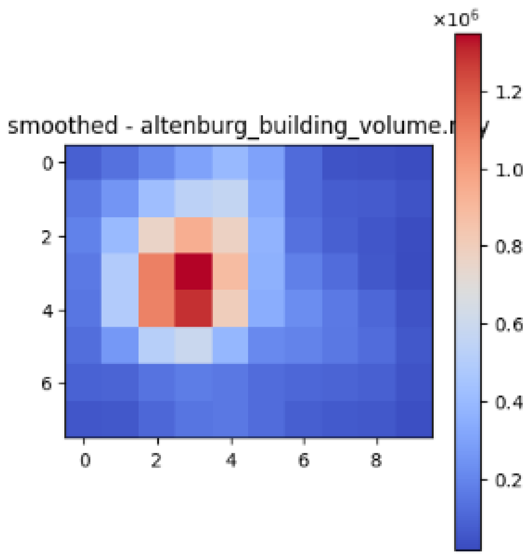 | 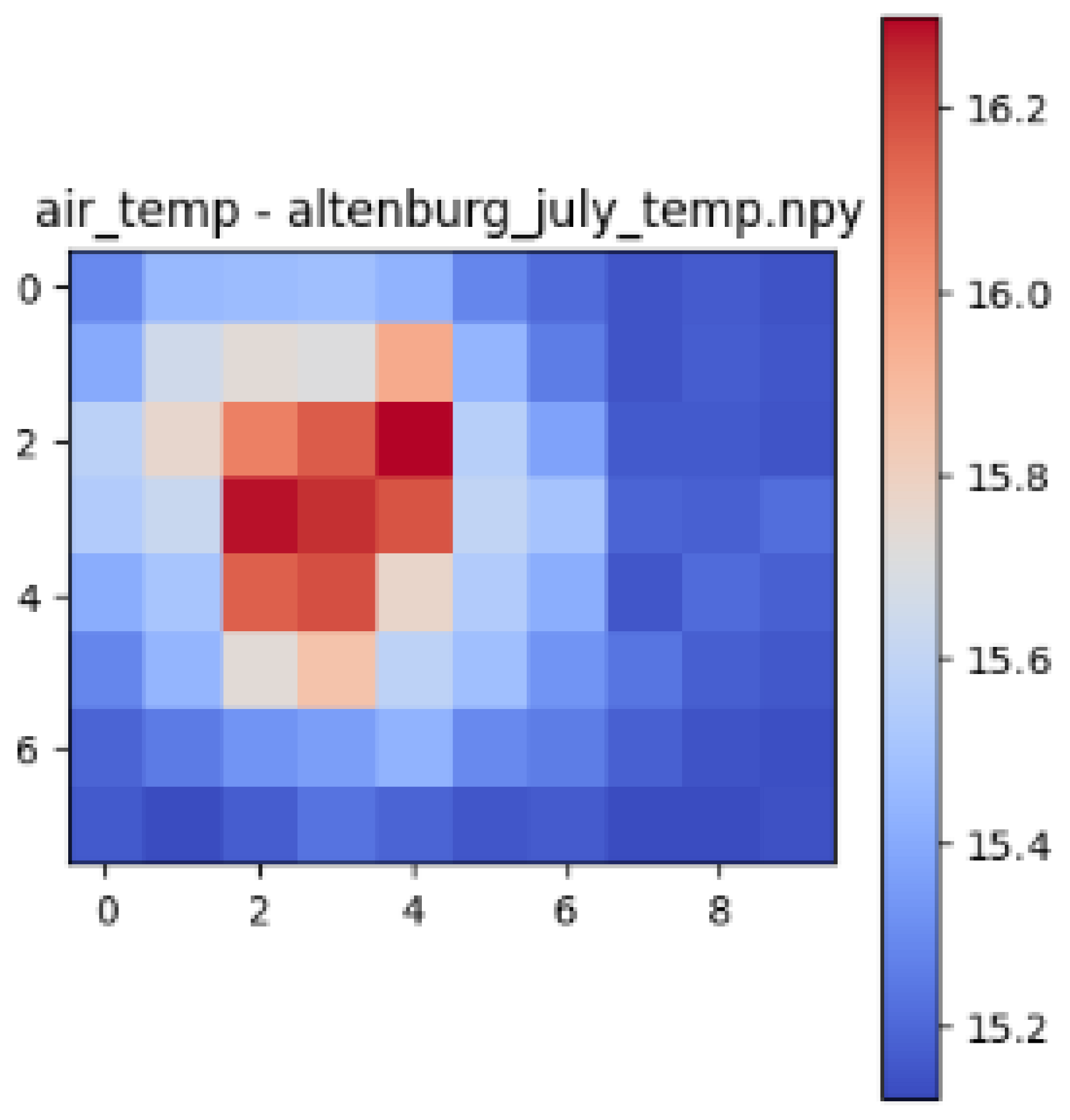 |
| Gera | 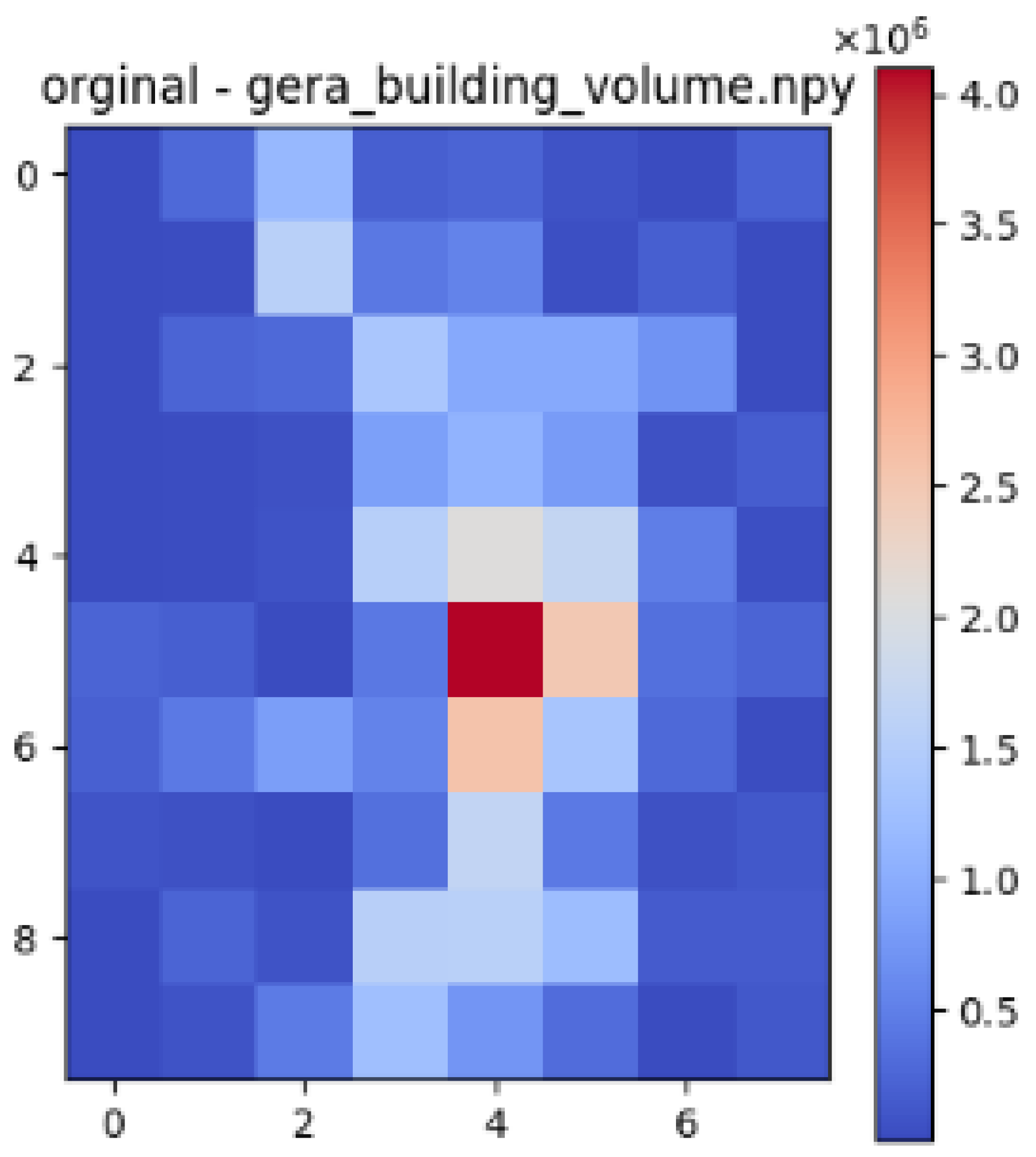 | 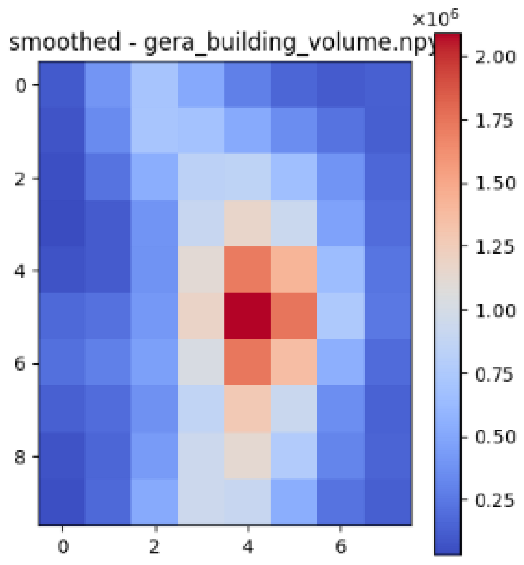 | 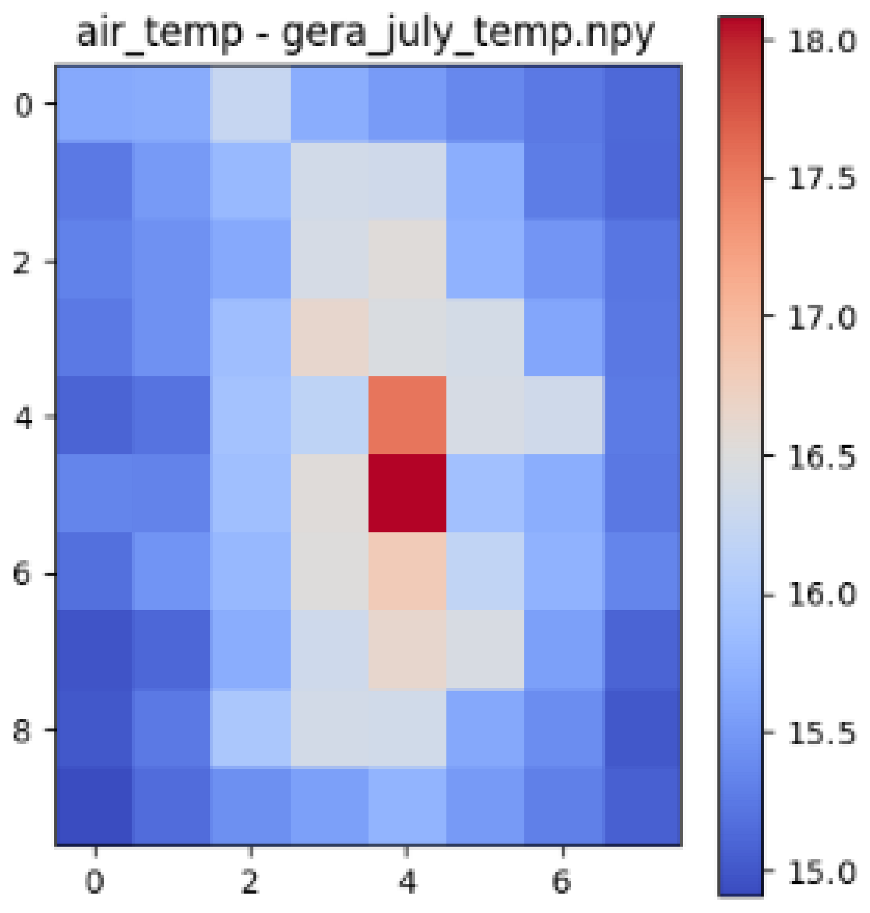 |
| Jena | 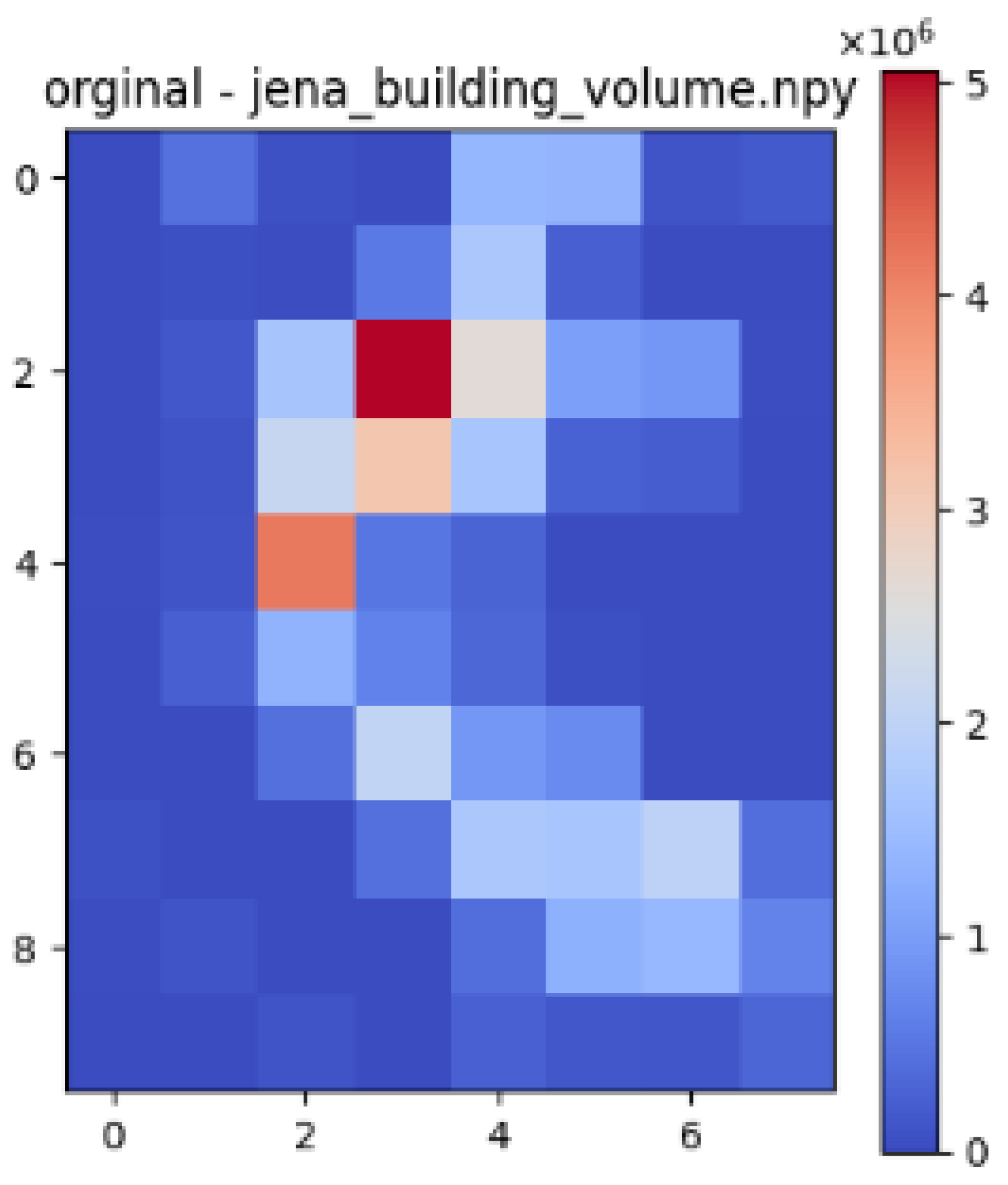 | 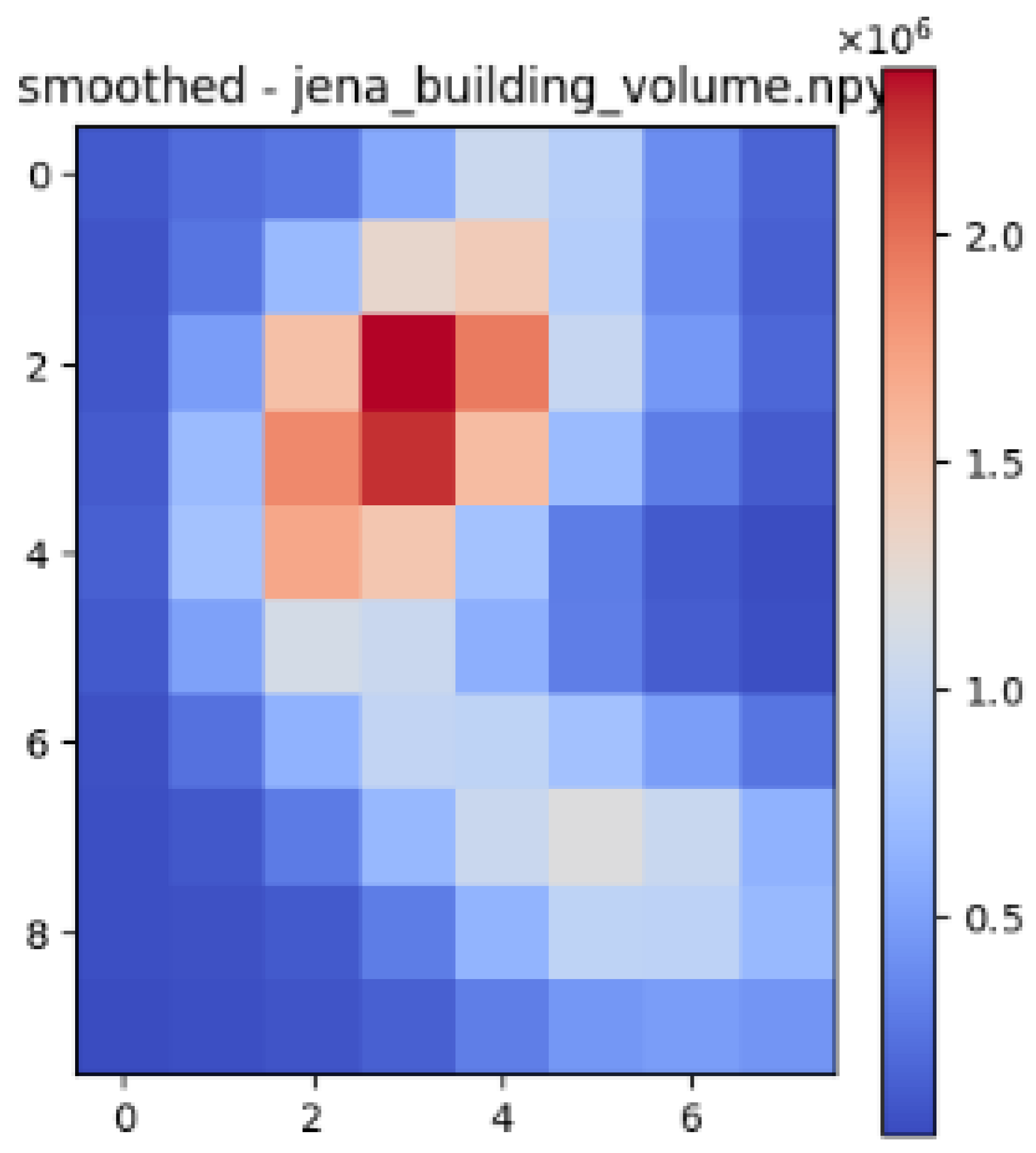 |  |
| Sonneberg |  | 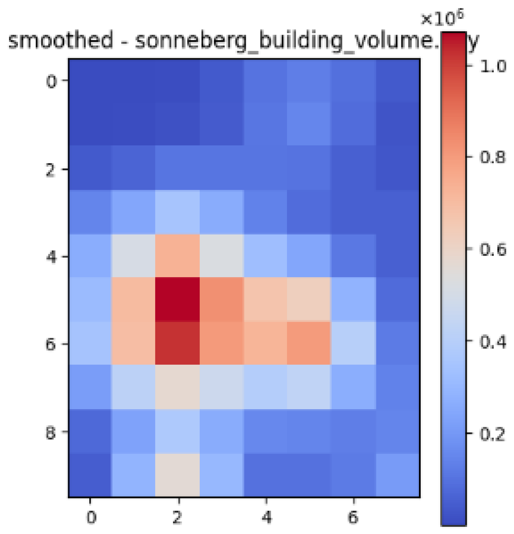 | 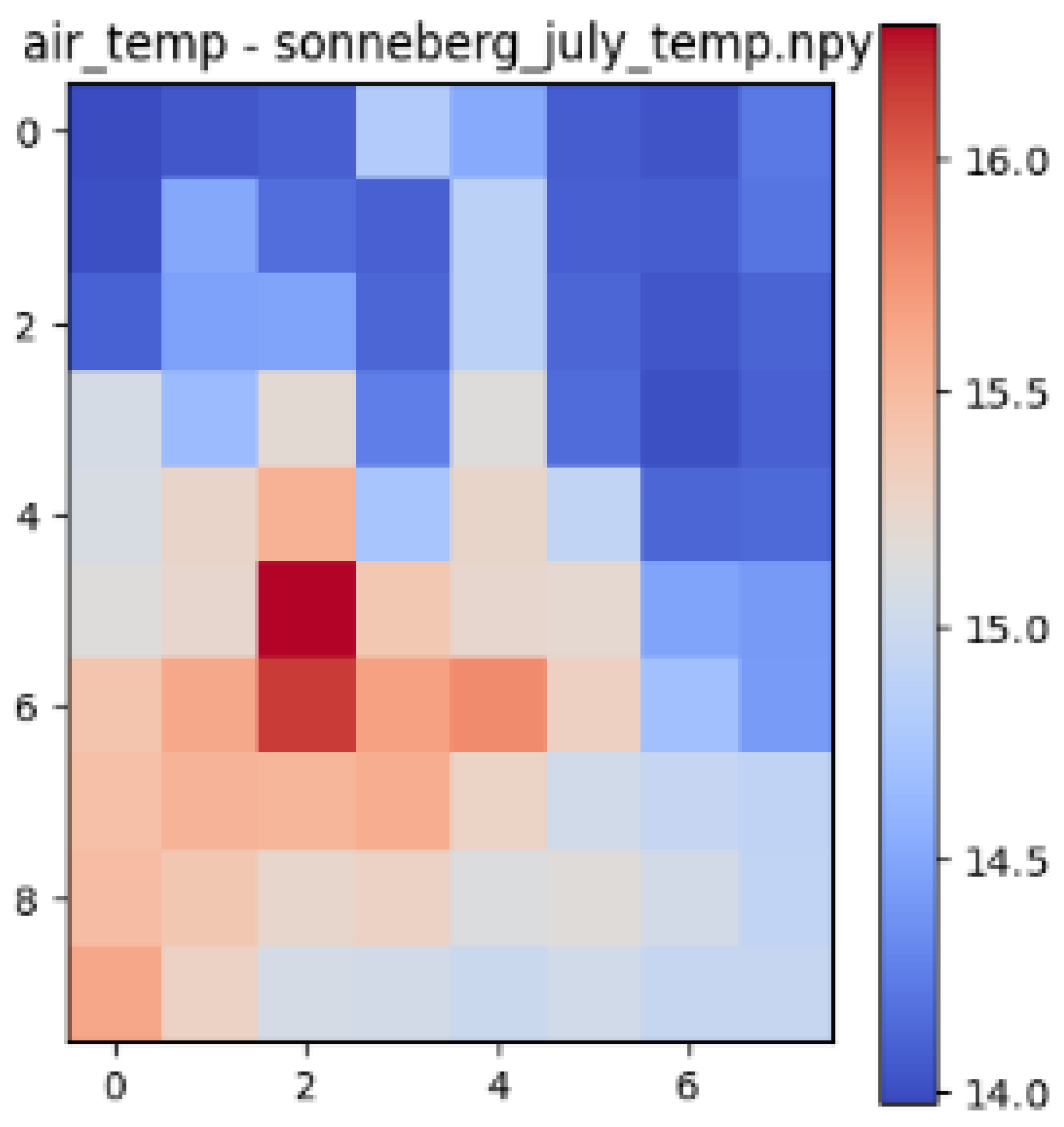 |
| Dataset | Random Forest | XGBoost | ||
|---|---|---|---|---|
| SSIM | LPIPS | SSIM | LPIPS | |
| Altenburg | 0.89 | 0.0000059 | 0.74 | 0.0000183 |
| Erfurt | 0.82 | 0.0000504 | 0.71 | 0.0002 |
| Gera | 0.88 | 0.0000377 | 0.72 | 0.0001 |
| Gotha | 0.80 | 0.0000479 | 0.77 | 0.0000430 |
| Jena | 0.77 | 0.00014 | 0.61 | 0.0003 |
| Schmalkalden | 0.70 | 0.0000479 | 0.47 | 0.0001 |
| Sondershausen | 0.65 | 0.0001 | 0.45 | 0.0002 |
| Sonneberg | 0.65 | 0.0001 | 0.46 | 0.0001 |
| Suhl | 0.62 | 0.0001 | 0.46 | 0.0002 |
| Weimar | 0.80 | 0.0000924 | 0.71 | 0.0001 |
| Ground Truth Air Temperature Map | Predicted Air Temperature Map | Difference Between Ground Truth and Predictions | |
|---|---|---|---|
| Sonneberg | 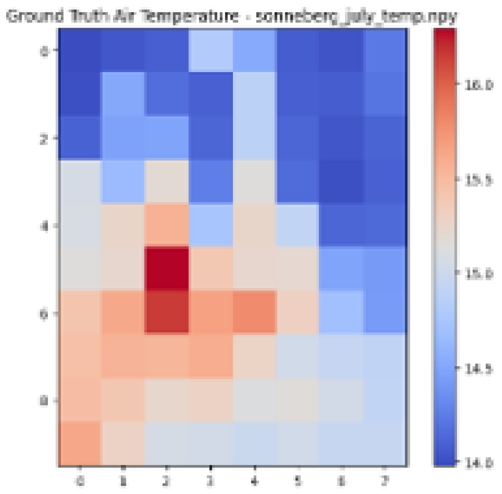 | 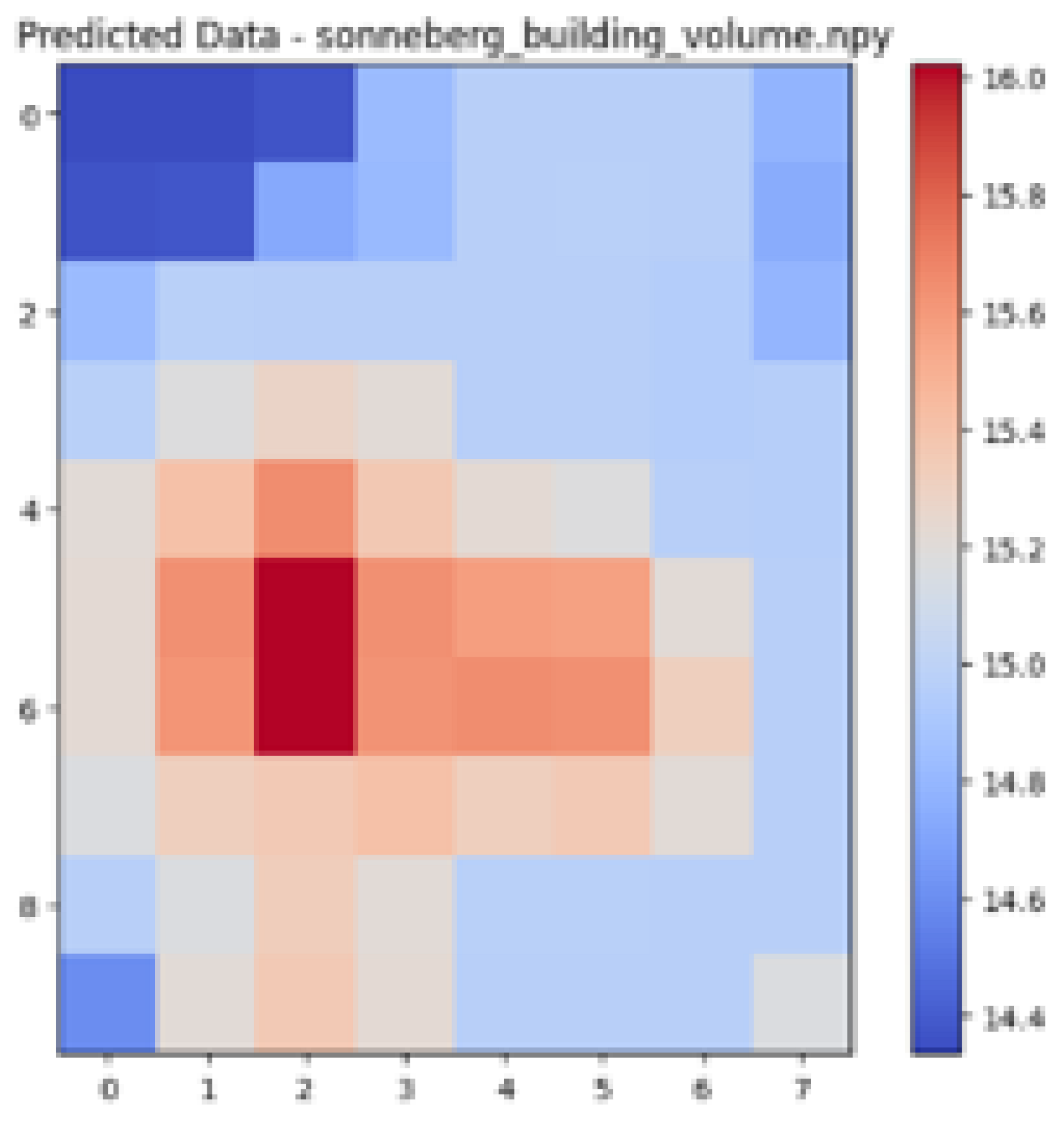 |  |
| Erfurt | 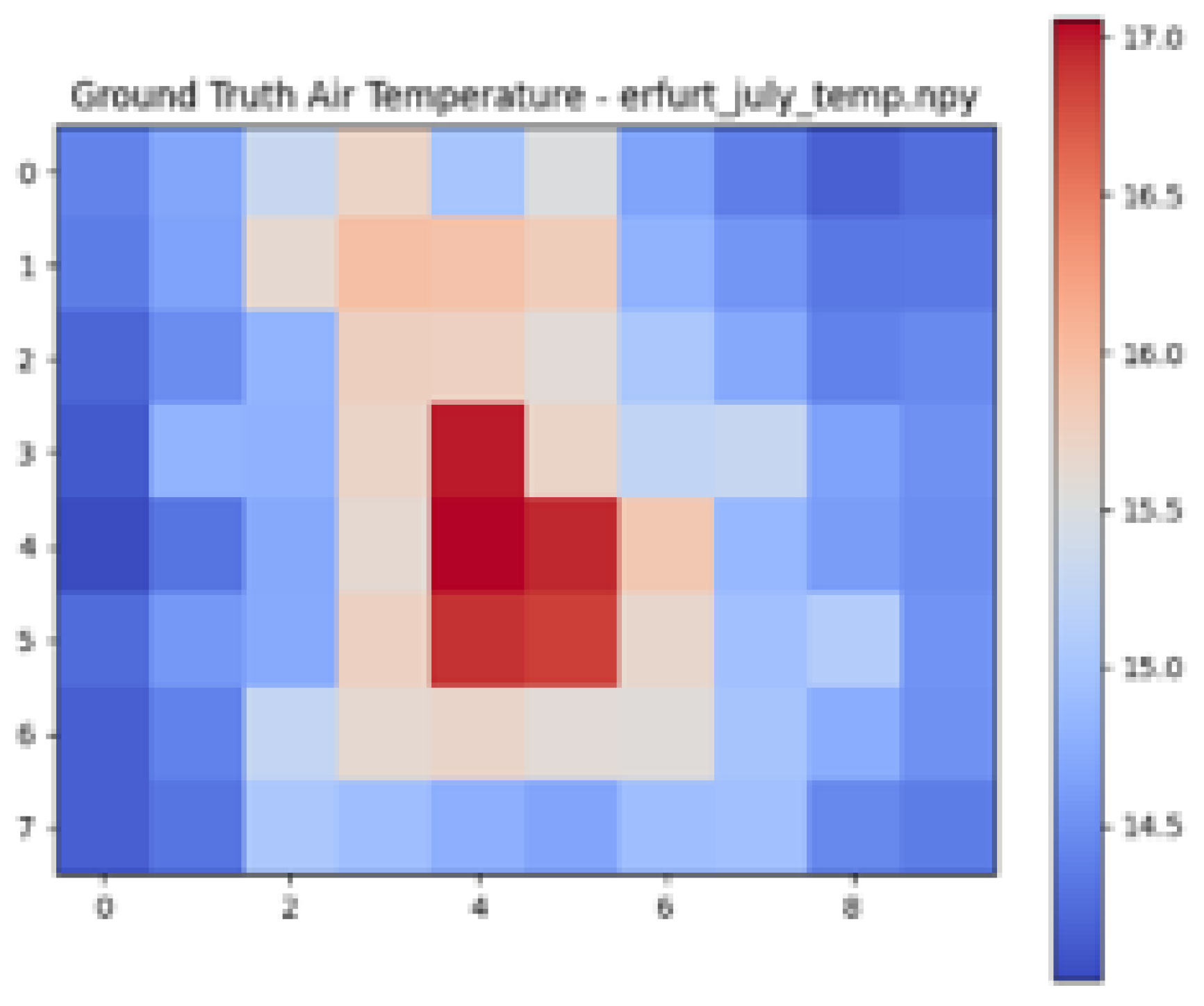 | 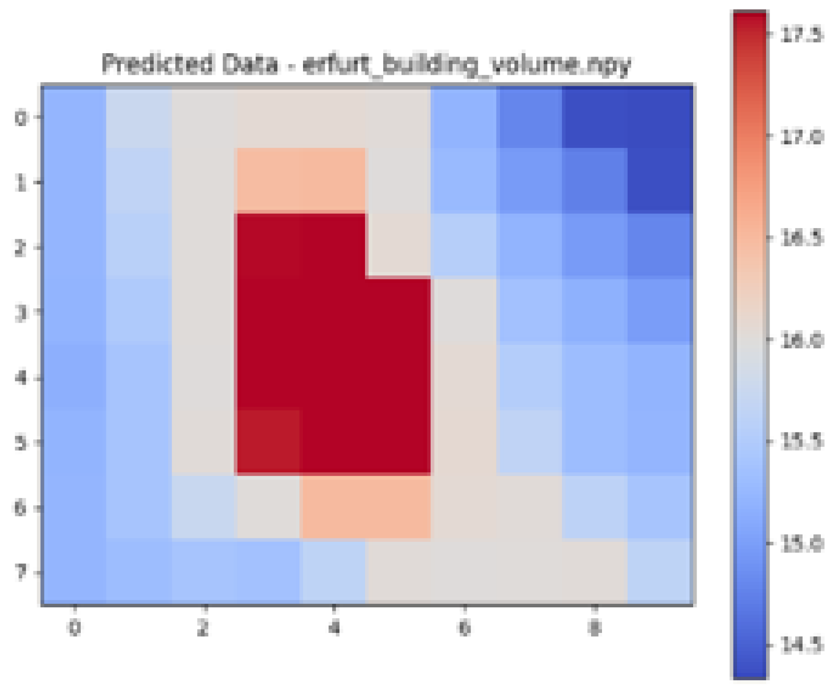 | 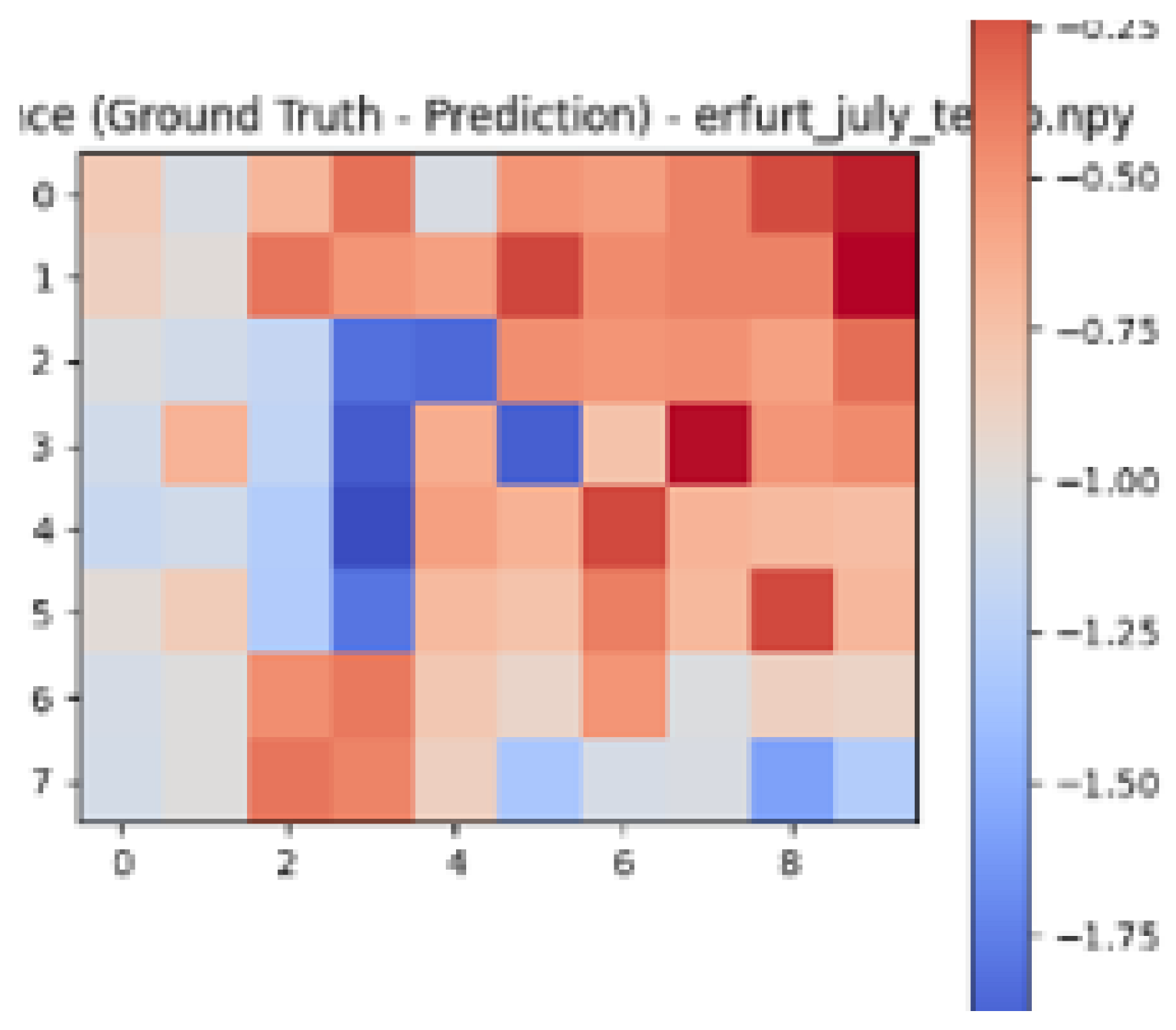 |
| Suhl | 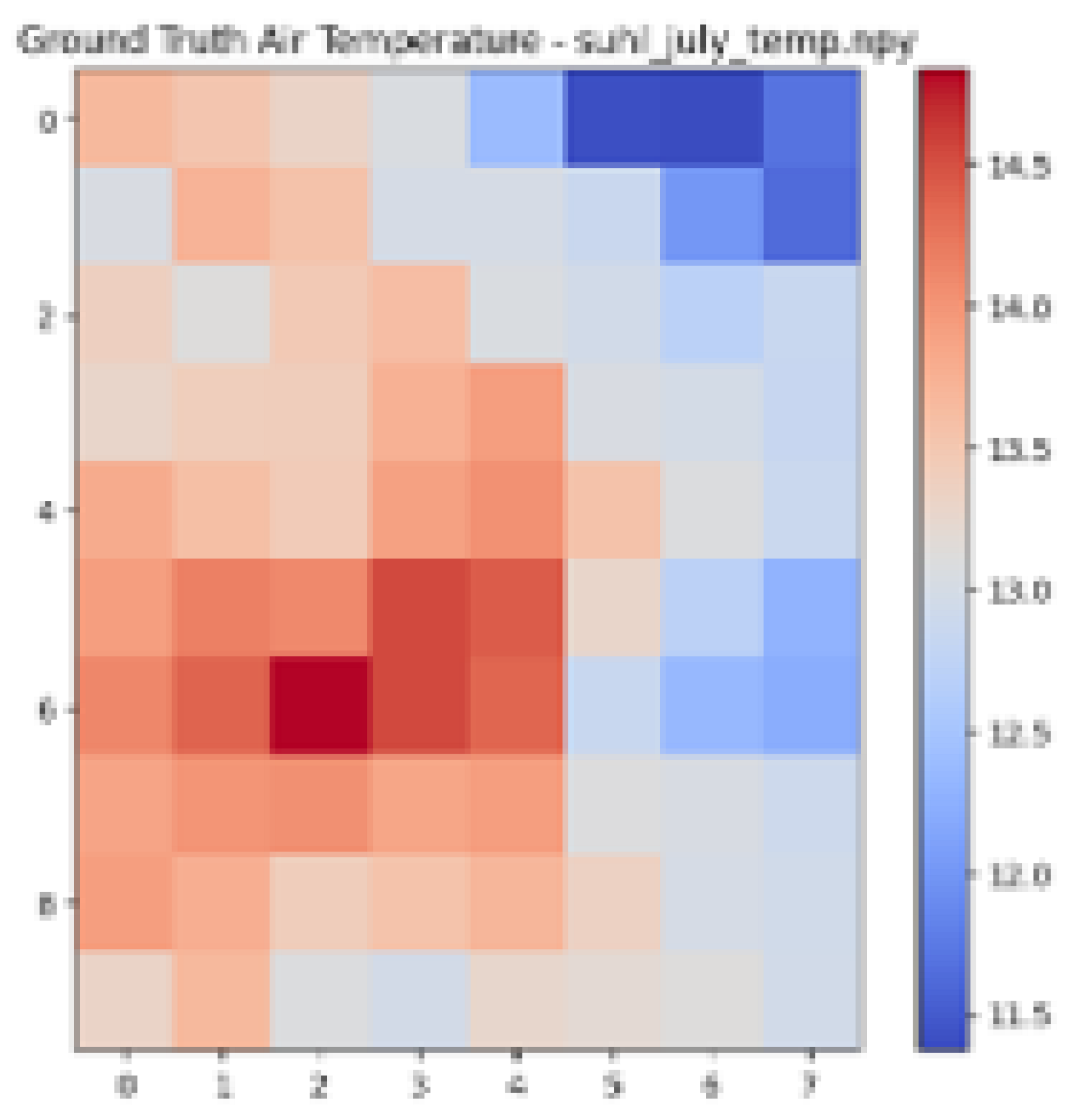 | 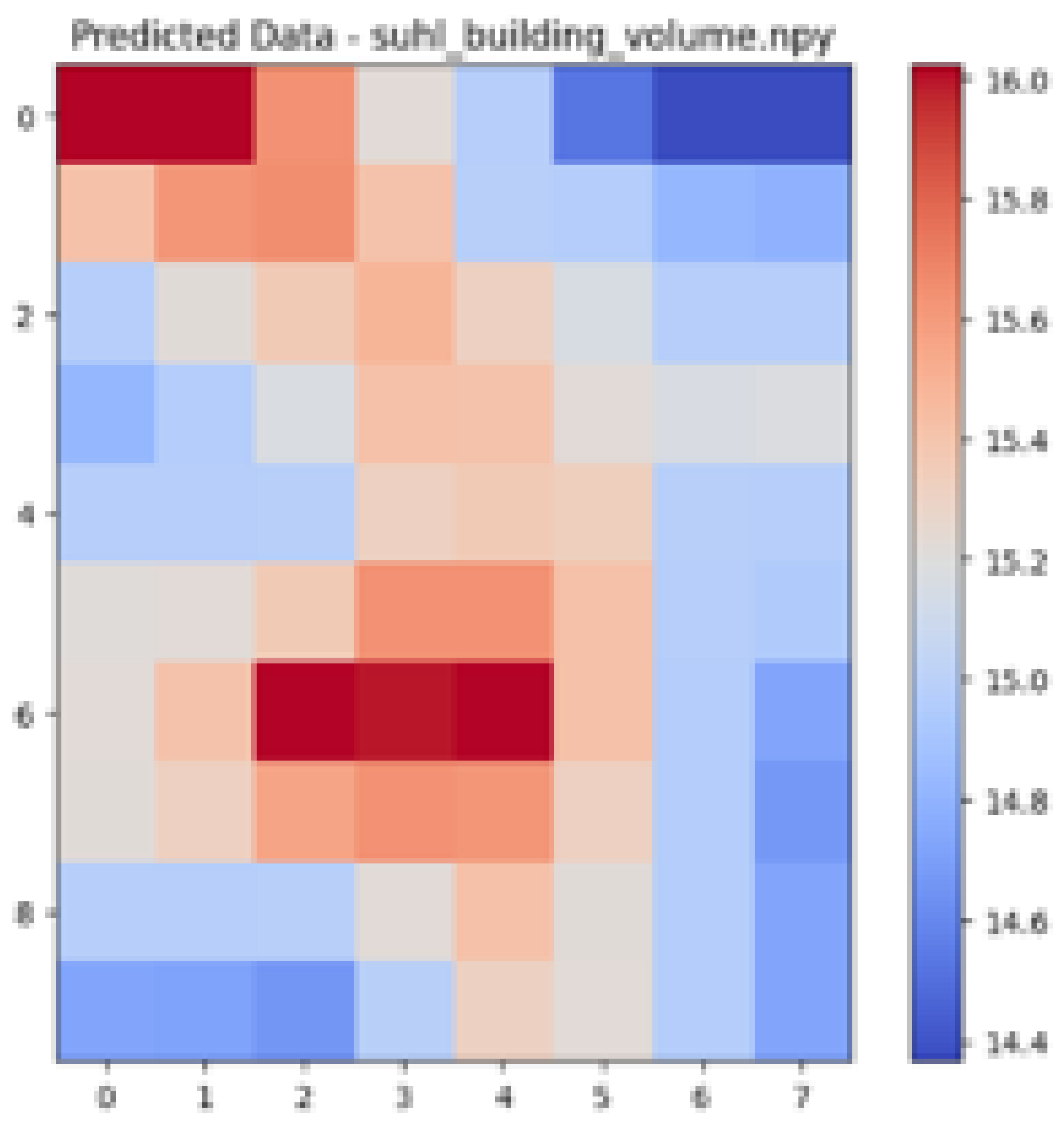 |  |
| Ground Truth Air Temperature Map | Predicted Air Temperature Map | Difference Between Ground Truth and Predictions | |
|---|---|---|---|
| Sondershausen | 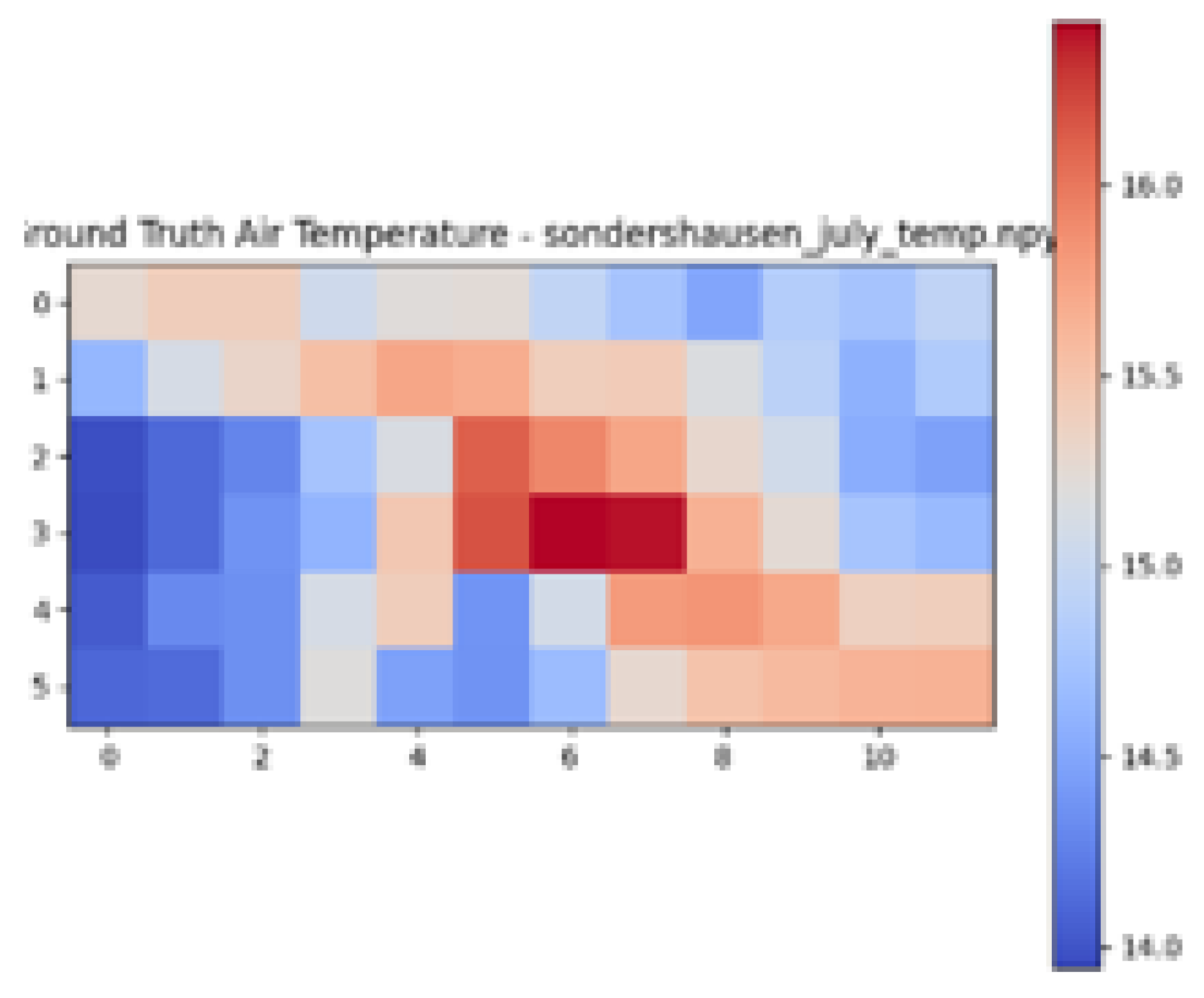 | 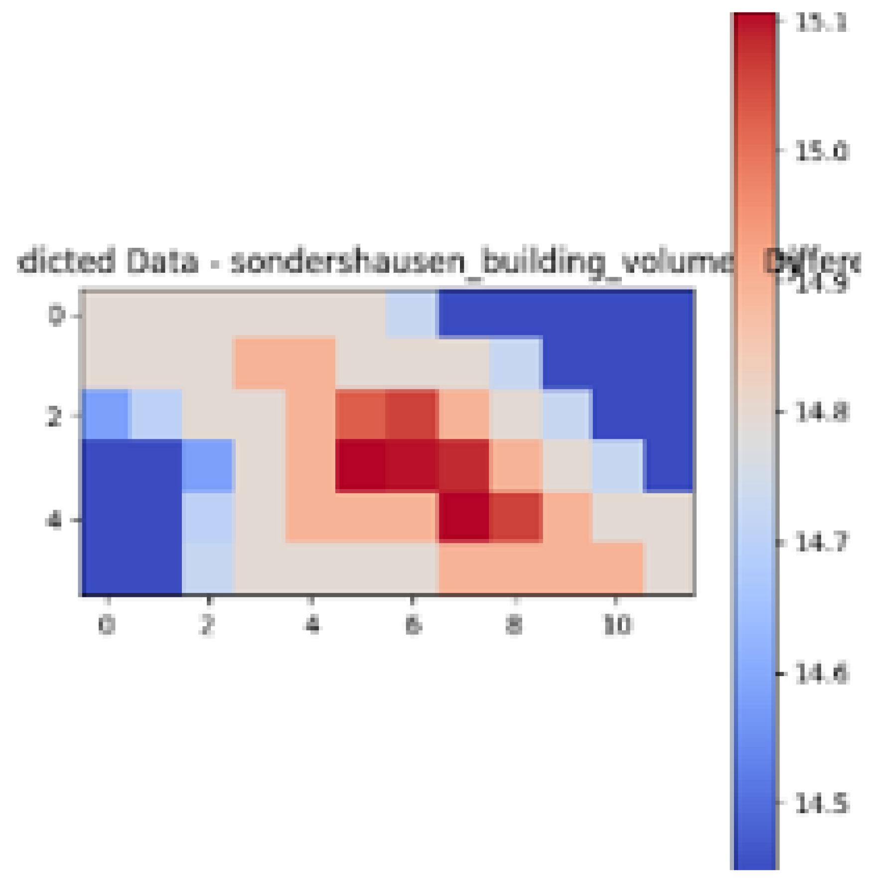 |  |
| Erfurt |  |  | 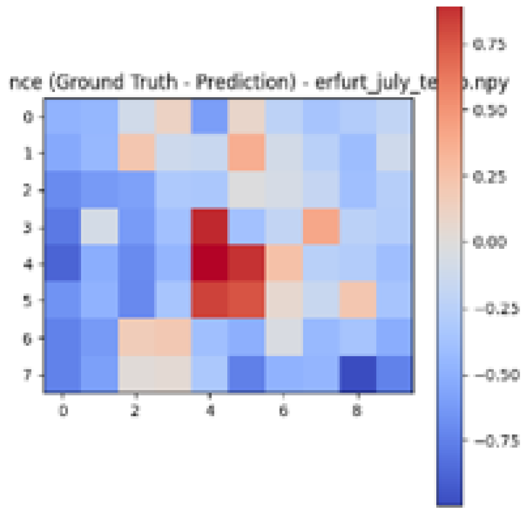 |
| Schmalkalden | 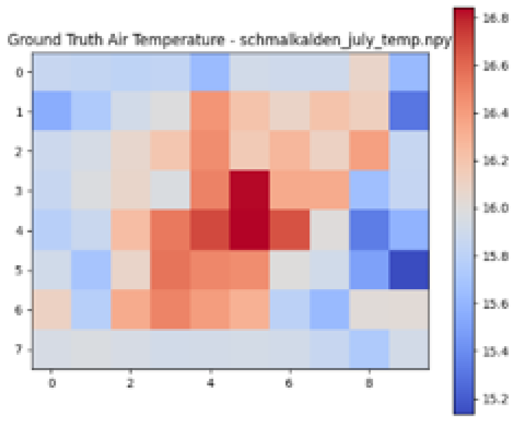 | 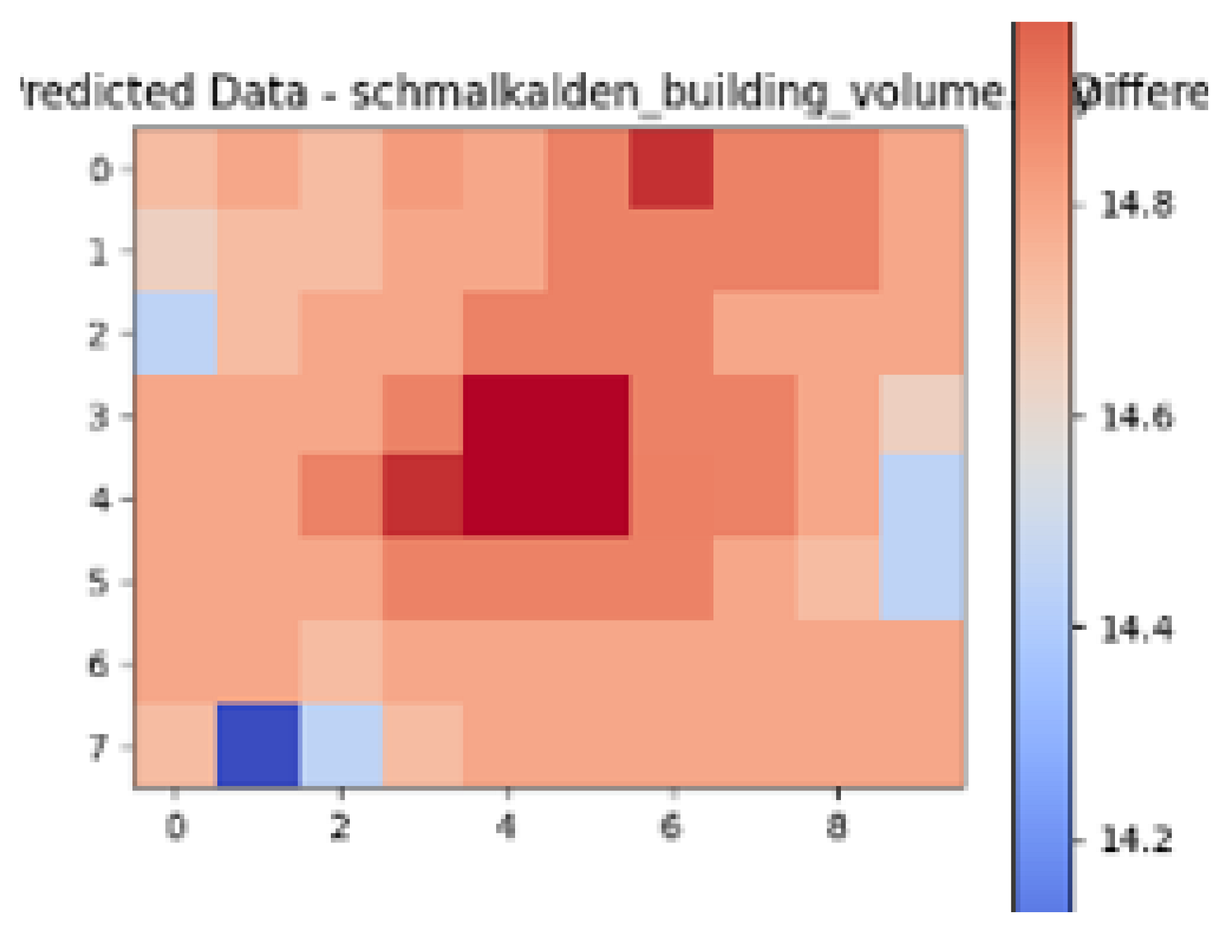 |  |
Disclaimer/Publisher’s Note: The statements, opinions and data contained in all publications are solely those of the individual author(s) and contributor(s) and not of MDPI and/or the editor(s). MDPI and/or the editor(s) disclaim responsibility for any injury to people or property resulting from any ideas, methods, instructions or products referred to in the content. |
© 2025 by the authors. Licensee MDPI, Basel, Switzerland. This article is an open access article distributed under the terms and conditions of the Creative Commons Attribution (CC BY) license (https://creativecommons.org/licenses/by/4.0/).
Share and Cite
Kıvılcım, B.; Bradley, P.E. A Data-Driven Approach for Urban Heat Island Predictions: Rethinking the Evaluation Metrics and Data Preprocessing. Urban Sci. 2025, 9, 151. https://doi.org/10.3390/urbansci9050151
Kıvılcım B, Bradley PE. A Data-Driven Approach for Urban Heat Island Predictions: Rethinking the Evaluation Metrics and Data Preprocessing. Urban Science. 2025; 9(5):151. https://doi.org/10.3390/urbansci9050151
Chicago/Turabian StyleKıvılcım, Berk, and Patrick Erik Bradley. 2025. "A Data-Driven Approach for Urban Heat Island Predictions: Rethinking the Evaluation Metrics and Data Preprocessing" Urban Science 9, no. 5: 151. https://doi.org/10.3390/urbansci9050151
APA StyleKıvılcım, B., & Bradley, P. E. (2025). A Data-Driven Approach for Urban Heat Island Predictions: Rethinking the Evaluation Metrics and Data Preprocessing. Urban Science, 9(5), 151. https://doi.org/10.3390/urbansci9050151