Article

Weather Forecasting Using Radial Basis Function Neural Network in Warangal, India

by
Venkataramana Veeramsetty
1,
Prabhu Kiran
2,
Munjampally Sushma
2 and
Surender Reddy Salkuti
3,*
1
Center for AI and Deep Learning, Department of Electrical and Electronics Engineering, SR University, Warangal 506371, India
2
Department of Electrical and Electronics Engineering, SR University, Warangal 506371, India
3
Department of Railroad and Electrical Engineering, Woosong University, Daejeon 34606, Republic of Korea
*
Author to whom correspondence should be addressed.
Urban Sci. 2023, 7(3), 68; https://doi.org/10.3390/urbansci7030068
Submission received: 25 March 2023 / Revised: 2 June 2023 / Accepted: 16 June 2023 / Published: 21 June 2023

Abstract

:
Weather forecasting is an essential task in any region of the world for proper planning of various sectors that are affected by climate change. In Warangal, most sectors, such as agriculture and electricity, are mainly influenced by climate conditions. In this study, weather (WX) in the Warangal region was forecast in terms of temperature and humidity. A radial basis function neural network was used in this study to forecast humidity and temperature. Humidity and temperature data were collected for the period of January 2021 to December 2021. Based on the simulation results, it is observed that the radial basis function neural network model performs better than other machine learning models when forecasting temperature and humidity.

1. Introduction

The daily atmospheric fluctuation is called weather (WX). WX forecasting, as a vital and necessary function in people’s everyday lives, analyzes changes in the existing state of the atmosphere. It is a critical activity that impacts many areas such as agriculture [1,2,3], irrigation [4], and the marine trade [5], and it has the potential to save many lives from unanticipated mishaps [6]. It is described as the examination of atmospheric factors such as temperature [7,8], irradiation [9,10,11,12,13,14], airflow, wind speed [15,16], wind direction, humidity [17], precipitation [18], and rainfall [19]. Forecast precision can be affected by a variety of circumstances. Season, geographical location, input data accuracy, WX classifications, lead time, and validity time are some of these effective elements [20,21].
Warangal is the ancient capital of the Kakatiyas Dynasty and currently one of the major cities in Telangana State, India. The Warangal district map is shown in Figure 1. It is spread over 1766 square kilometers. According to the 2011 census (https://warangal.telangana.gov.in/ (accessed on 12 March 2023)) Warangal has a population of 890,651 people. Agriculture is the most important economic sector, with irrigation mostly dependent on monsoon and seasonal rainfalls. Paddy, cotton, mango, and wheat are the most important crops. In addition to rainfall, crops also grow with groundwater using pumps that require electricity. WX forecasting is very important in this region as it affects agricultural yield and the load on the electric substations.

2. Literature Review

WX forecast provide essential information about future WX conditions [22]. WX forecasting employs various methodologies, ranging from basic sky observations to complex computerized mathematical models. Presently, WX forecasts are primarily based on physical computer models that utilize discrete numerical grids to solve governing equations. Overall, this approach has been highly successful. However, many important applications still face limitations with current numerical WX prediction (NWP) models [23,24,25]. Initially, linear techniques and machine learning approaches were used for WX forecasting over NWP [26]. For instance, solar irradiation was forecast using a multiple linear regression model [27], while support vector machines were employed for predicting solar power generation [28]. Neural networks were utilized for precipitation forecasting [29], and their performance was compared to linear regression models.
In Beijing, surface temperature, humidity, wind speed, and wind direction at 24 automatic WX stations were forecast using an ensemble of a spatial–temporal attention network and multi-layer perceptron [30]. In Göztepe, İstanbul, a neuro-fuzzy network and ARIME model-based approach were used for WX forecasting [31]. Temporal convolutional neural networks were implemented for WX forecasting [32], while photovoltaic power generation was predicted using a sequential model, namely long short-term memory [33]. All these works have made valuable contributions to WX forecasting using machine learning models such as artificial neural networks, convolutional neural networks, linear regression, and support vector machines.
This study focused on forecasting two WX parameters: temperature and humidity. The values of temperature and humidity from one hour and one day prior, as well as the season, were used as input features for temperature (Temp(T)) and humidity (Humd(T)) prediction. Therefore, the input features for forecasting temperature and humidity include Temp(T-1), Temp(T-24), Humd(T-1), Humd(T-24), and Season. A radial basis function neural network (RBFNN) [34] was employed to forecast the WX in terms of temperature and humidity. The optimal RBFNN model was identified by tuning hyperparameters such as the number of centroids and the width parameter. The best model was determined based on the lowest mean square error on the validation data.
The remaining sections of the paper are organized as follows: Section 2 explains the data analytics, RBFNN architecture, and its training algorithm. Section 3 presents the simulation results, and Section 4 discusses the conclusions of this work, and Appendix A describes sample radial basis function neural network (RBFNN) architecture, and Appendix A.1 presents unsupervised learning between input and hidden layers of RBFNN, and Appendix A.2 presents supervised learning between output and hidden layer of RBFNN, and Appendix B explains prediction using trained RBFNN.

3. Materials and Methods

This section provides a detailed explanation of the analytics conducted on the temperature and humidity data collected in the Warangal region from January 2021 to December 2021. It also describes the architecture of the radial basis function neural network (RBFNN) and the training procedure.

3.1. Temperature Dataset

The temperature dataset consists of a total of 5 input features: Temp(T-1), Temp(T-24), Humd(T-1), Humd(T-24), and season. The dataset also includes one output label, Temp(T). The data for this dataset were obtained and arranged from the source available at https://data.mendeley.com/datasets/tj54nv46hj (accessed on 28 August 2022). A few sample entries from the temperature dataset are presented in Table 1. Statistical information such as the mean, standard deviation, minimum, and maximum values of the temperature dataset can be found in Table 2.

3.2. Humidity Dataset

The humidity dataset also comprises 5 input features: Temp(T-1), Temp(T-24), Humd(T-1), Humd(T-24), and season, which are the same as the temperature dataset. However, the output label for the humidity dataset is different, namely Humd(T). A selection of sample entries from the humidity dataset is presented in Table 3. Statistical information, including the mean, standard deviation, minimum, and maximum values of the humidity dataset, can be found in Table 4.

3.3. Data Pre-Processing

The temperature and humidity data underwent several data pre-processing techniques, including missing value treatment, outlier data treatment, normalization, and data splitting. The missing value information for each column in the dataset is presented in Table 5. It can be observed from Table 5 that there are no missing values in the data.
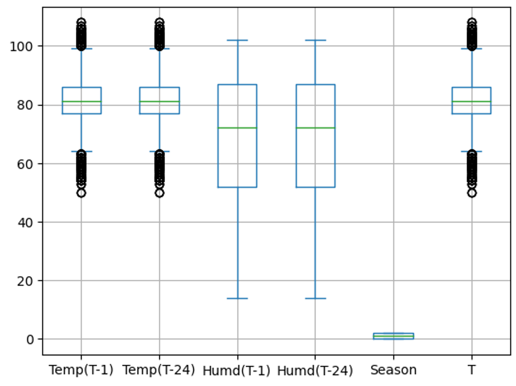
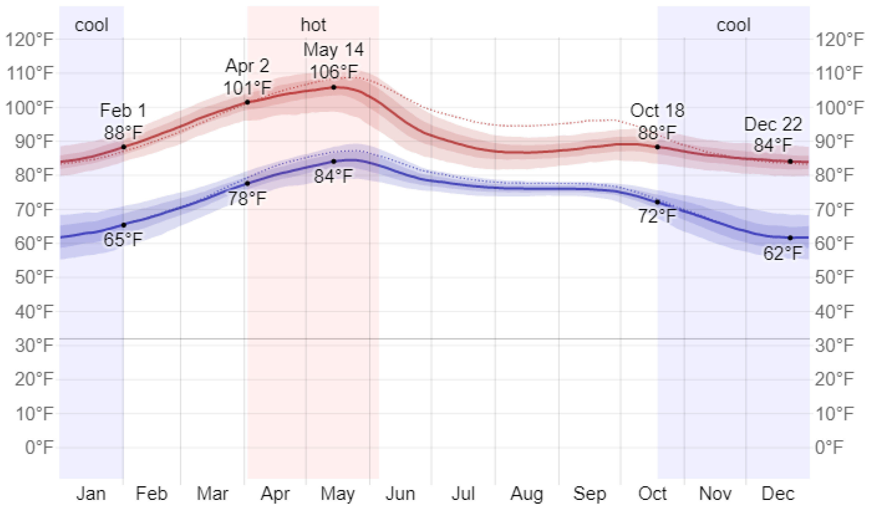
The box plot for each feature in the temperature dataset is depicted in Figure 2. This box plot helps visualize any outliers present in the data. It can be observed from the box plot that there are a few outlier samples; however, these outliers are not considered actual outliers. The samples fall outside the box due to the significant variation in the data from the winter season to the summer season in Warangal, as illustrated in Figure 3.
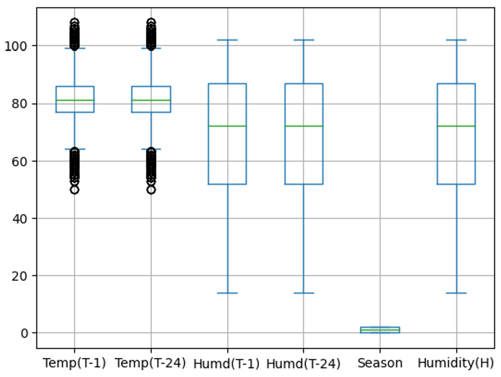
Similarly, the box plot for each feature in the humidity dataset is presented in Figure 4. This box plot is used to identify any outliers in the data.
Data normalization was implemented on the data using Equation (1) in order to reduce data redundancy in a table and improve data integrity.
D a t a n o r m = D a t a D a t a m i n D a t a m a x D a t a m i n
Finally, the data were randomly divided into training and testing sets to train and validate the radial basis function neural network (RBFNN). As part of the data split, 5853 samples were used for training, and 2883 samples were used for testing.

3.4. Radial Basis Function Neural Network (RBFNN)

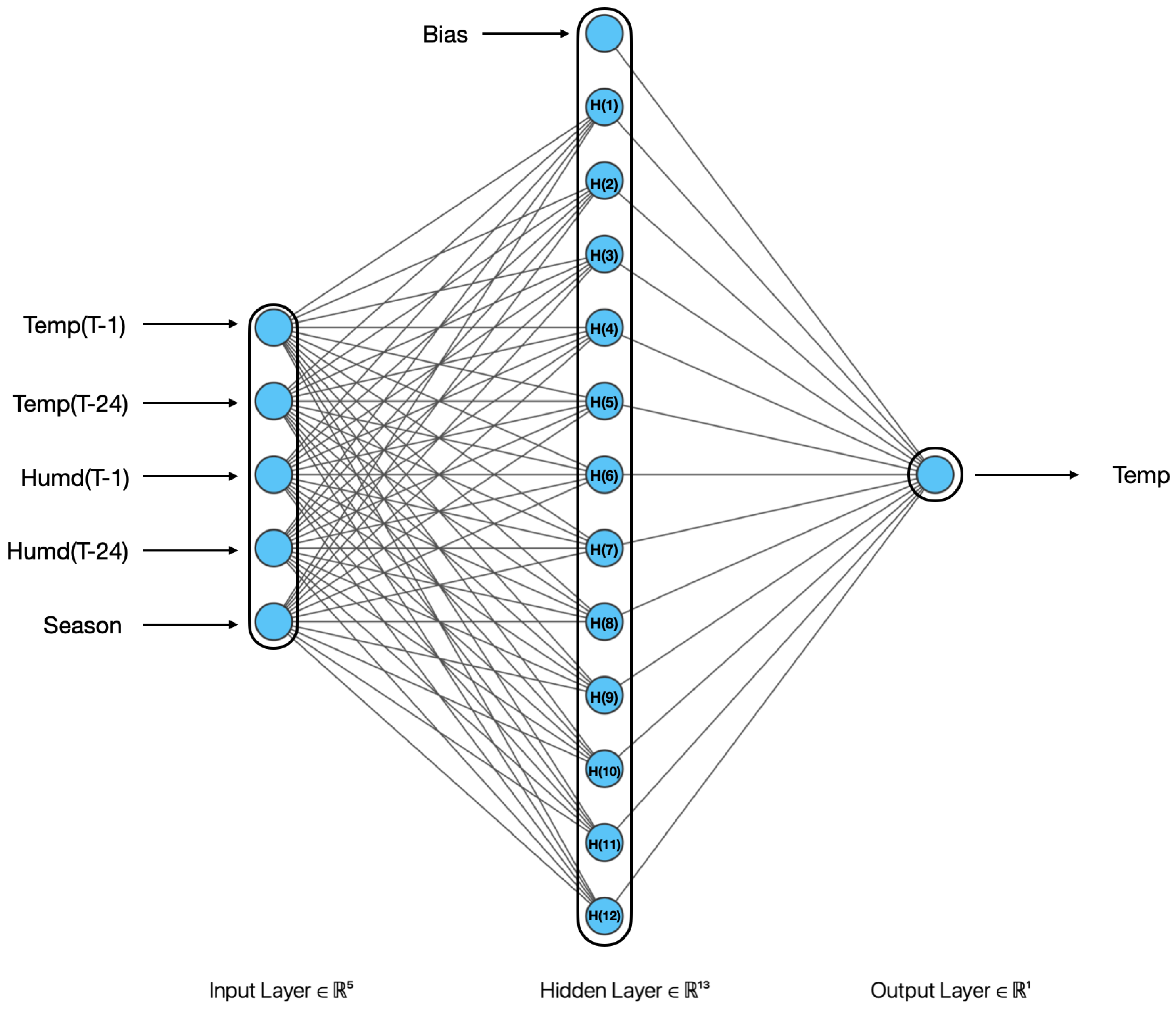
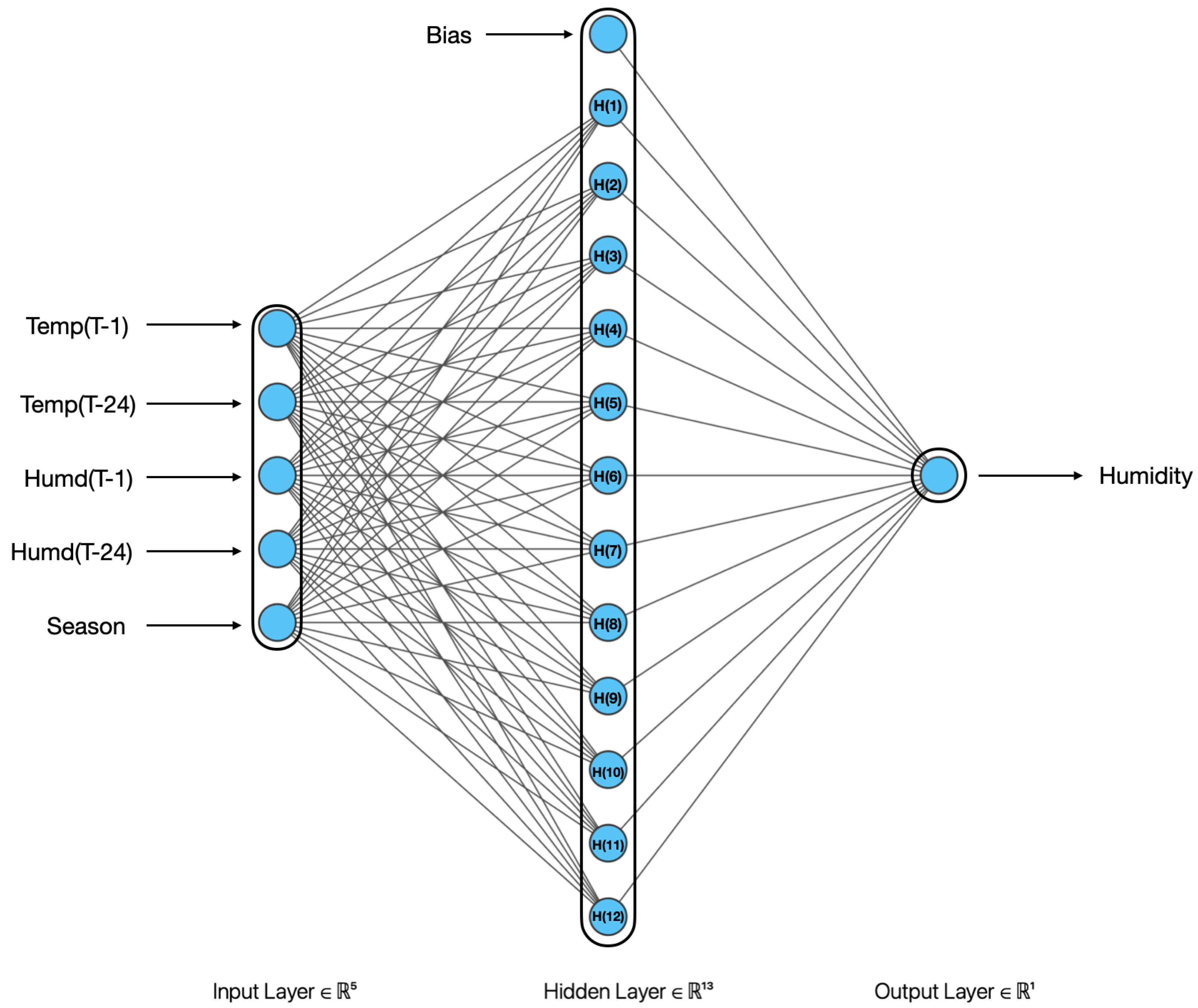
The RBFNN consists of one input layer, one hidden layer, and one output layer [35,36,37]. The input layer comprises five neurons since temperature and humidity are forecast using five input features. The output layer consists of one neuron, as only either temperature or humidity is forecast by this model. The number of neurons in the hidden layer, also known as centroids, is a hyperparameter that will be tuned to obtain the best model. Unlike an ANN [38,39], the training of the RBFNN includes both supervised and unsupervised learning. The training between the input layer and hidden layer is based on unsupervised learning [40], while the training between the output layer and hidden layer is based on supervised learning. The hidden layer uses the Gaussian activation function [41], which is mathematically represented by Equation (2). The standard deviation σ [42] is calculated based on the width parameter “p” as shown in Equation (3). The RBFNN architecture for temperature forecasting is illustrated in Figure 5, and for humidity forecasting, it is depicted in Figure 6. The complete algorithm to train the RBFNN model using the stochastic gradient descent optimizer [43] is presented in Algorithm 1. The performance of the RBFNN is evaluated in terms of mean square error [44,45,46,47,48], as shown in Equation (4).
g ( x , μ , σ ) = e ( x μ ) 2 2 σ 2
σ ( p , μ i ) = 1 p ( μ i μ j ) 2
M S E = 1 n s a m p l e i = 1 n s a m p l e ( A c t u a l   l o a d P r e d i c t e d   l o a d ) 2
Algorithm 1 RBFNN training algorithm.
  Step 1: Read input and output features of temperature dataset ▹ X = {Temp(T-1), Temp(T-24), Humd(T-1), Humd(T-24), season} and Tempt(T), In case of humidity forecasting output is Humd(T) instead of Temp(T)
  Step 2: Initialize number of centriods (neurons) in hidden layer, weights W h k , bias parameter b k , learning rate η and tol = 1
  Step 3: Randomly pick few samples from training dataset and assign as mean vector ( μ ) for each neuron/centriod.
  while tol ≥ 0.001 do   ▹ Unsupervised learning between input and hidden layer of RBFNN
  Step 4: Calculate the euclidean distance (ED) between each sample and mean vector using Equation (5)
E D = ( X μ ) 2
  Step 5: Assign the sample which has minimum ED to that particular centroid and update mean value ( μ ) as an average of all assigned samples to that particular centroid.
  Step 6: Calculate tolerance (tol) as the maximum difference between old and new mean values among all centriods.
  end while
  Step 7: Calculate the standard deviation ( σ ) using Equation (6)
σ = 1 P ( j ϵ P _ n e i g h b o u r ( C i C j ) 2 )
  Step 8: Calculate the output of each hidden neuron (h) using Equation (7)
O h = exp ( X μ h ) 2 2 σ h 2
  while d e l W 0.001 do   ▹ Supervised learning between output and hidden layer of RBFNN
  Step 9: Calculate output of the RBFNN output layer using Equation (8)
O k = W h k T O h + b 0
  Step 10: Update W h k using Equation (9) and b k using (10)
W h k = W h k + η ( T e m p ( T ) O k ) O h
b o = b o + η ( T e m p ( T ) O k )
  Step 11: Find d e l W as maximum change among W h k and b k
  end while
  Step 12: Store model in terms of model parameters W h k , μ , σ and b k , and architecture

4. Results

The proposed RBFNN model was trained and tested using the temperature and humidity data collected from January 2021 to December 2021, comprising a total of 8736 samples. The model training and testing were implemented using Python programming in the Visual Studio environment, leveraging the specified dataset.

Optimal RBFNN Model to Forecast the Temperature

The RBFNN architecture with the minimum validation loss is considered the optimal model. Several RBFNN architectures are developed by tuning the number of centroids/neurons and the width parameter (P) in the hidden layer. The training and validation losses for different RBFNN architectures used for temperature forecasting are presented in Table 6 and Table 7, respectively. Among these architectures, the RBFNN model with 12 centroids and a width parameter of 11 was selected as the optimal model due to its lower validation loss of 0.0022, while the corresponding training loss is 0.0037.
The optimal RBFNN architecture for temperature forecasting, consisting of 12 centroids and a width parameter of 11, was trained using different batch sizes: 8, 16, 32, and 64. The convergence characteristics of the RBFNN architecture for these batch sizes are illustrated in Figure 7. It can be observed from the figure that the RBFNN model trained with a batch size of 32 achieves the minimum validation loss of 0.0022. Furthermore, the small difference between the training and validation losses indicates that the model is well trained without encountering underfitting or overfitting issues.
The training and validation losses for different RBFNN architectures used for humidity forecasting are presented in Table 8 and Table 9, respectively. Among these architectures, the RBFNN model with 12 centroids and a width parameter of 10 is considered the optimal model due to its lower validation loss of 0.0078. The corresponding training loss for this architecture is 0.011.
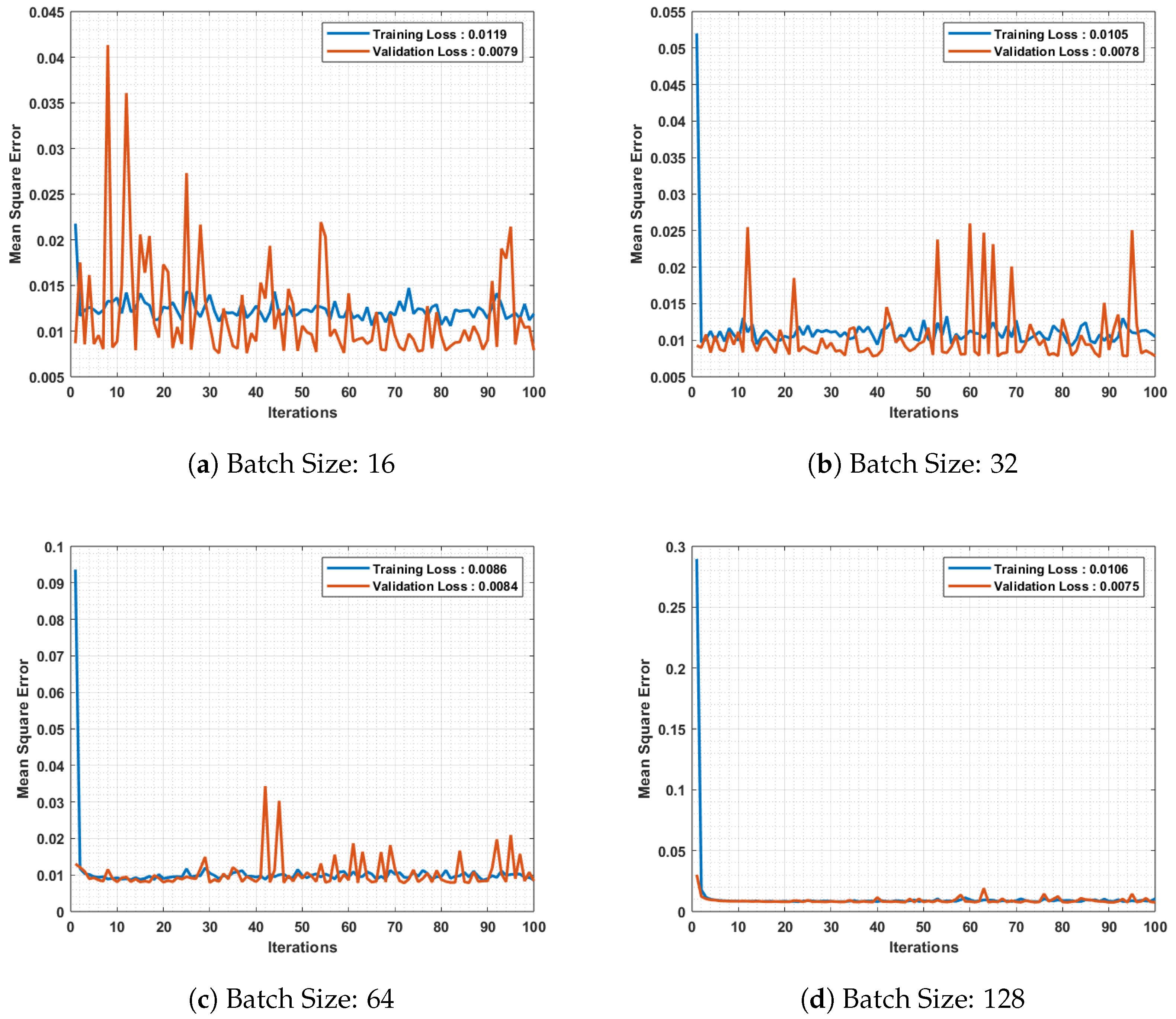
The optimal RBFNN architecture for humidity forecasting, consisting of 12 centroids and a width parameter of 10, was trained using different batch sizes: 16, 32, 64, and 128. The convergence characteristics of the RBFNN architecture for these batch sizes are illustrated in Figure 8. It can be observed from the figure that the RBFNN model trained with a batch size of 128 achieves the minimum validation loss of 0.0075. Additionally, the small difference between the training and validation losses indicates that the model is well trained without encountering underfitting or overfitting issues.
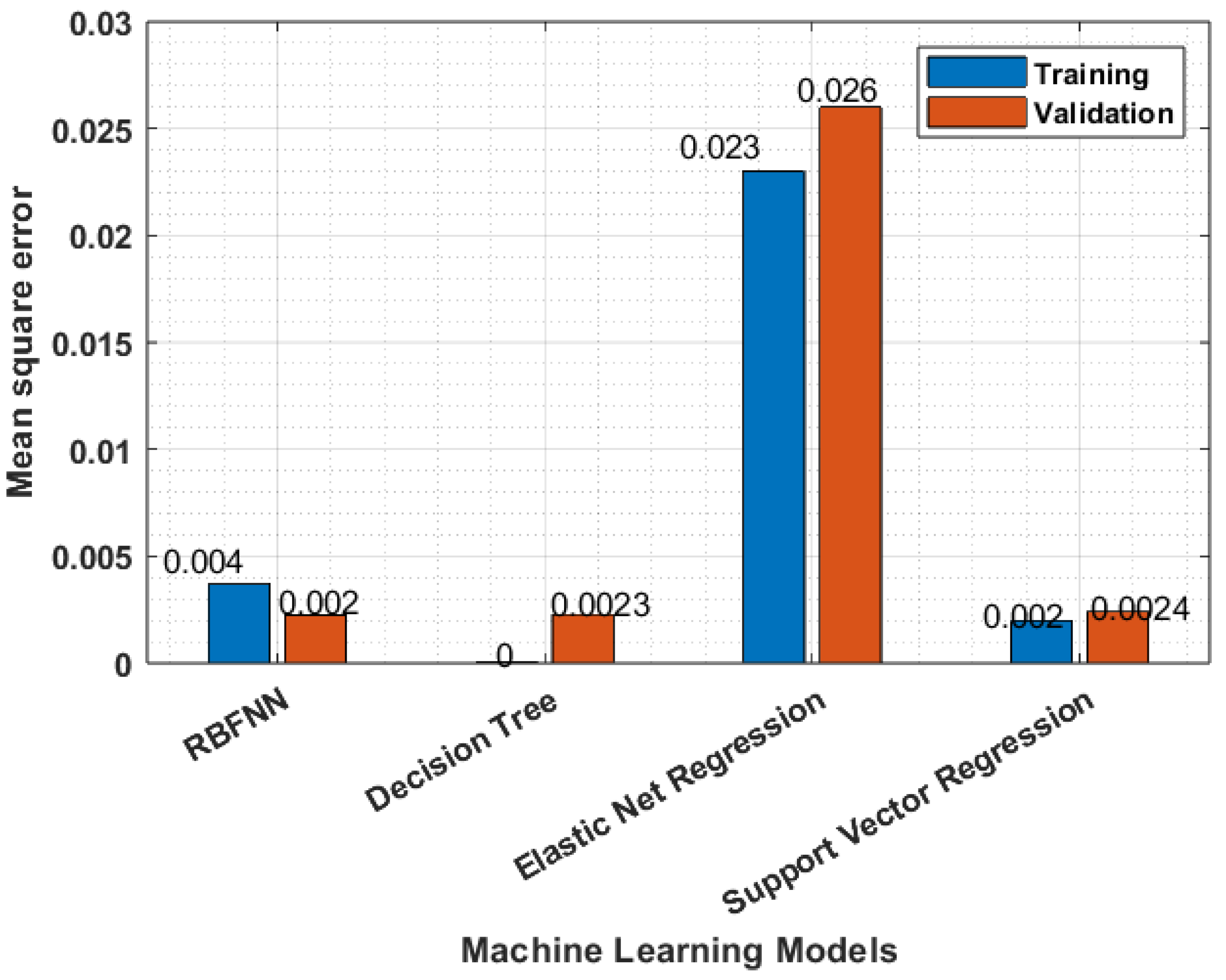
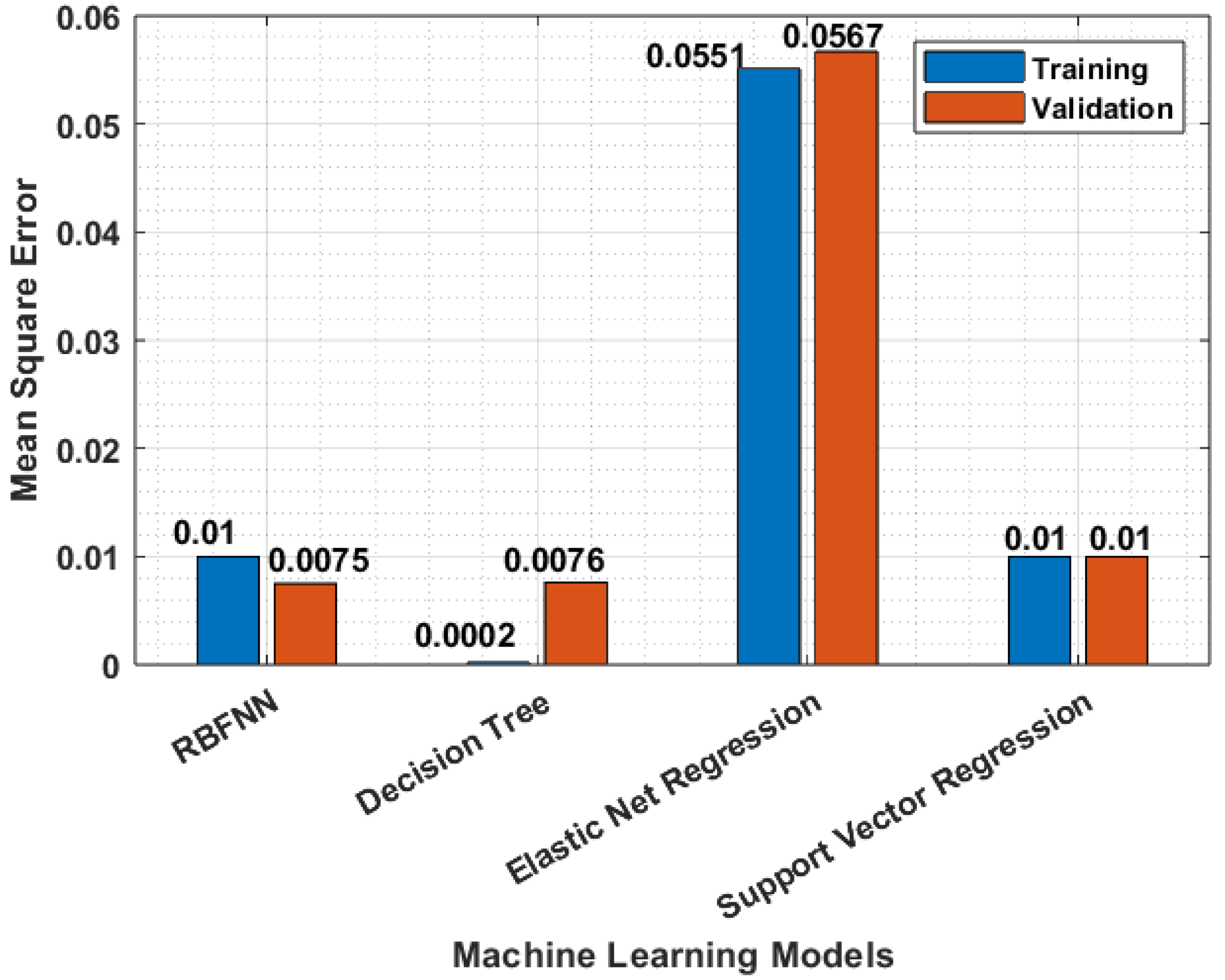
The performance of the RBFNN model for temperature forecasting was validated by comparing it with the decision tree model [49], support vector regression [50], and elastic net regression [51] in terms of training and validation losses, as shown in Figure 9. From Figure 9, it is observed that the RBFNN model has lower validation losses, while the decision tree model exhibits signs of overfitting. Similarly, the performance of the RBFNN model for humidity forecasting was validated by comparing it with the decision tree model in terms of training and validation losses, as shown in Figure 10. From Figure 10, it is observed that the RBFNN model achieves lower validation losses compared to the decision tree model. Additionally, the decision tree model shows signs of overfitting. These comparisons demonstrate the superior performance of the RBFNN model over the decision tree model in terms of validation losses for both temperature and humidity forecasting tasks.
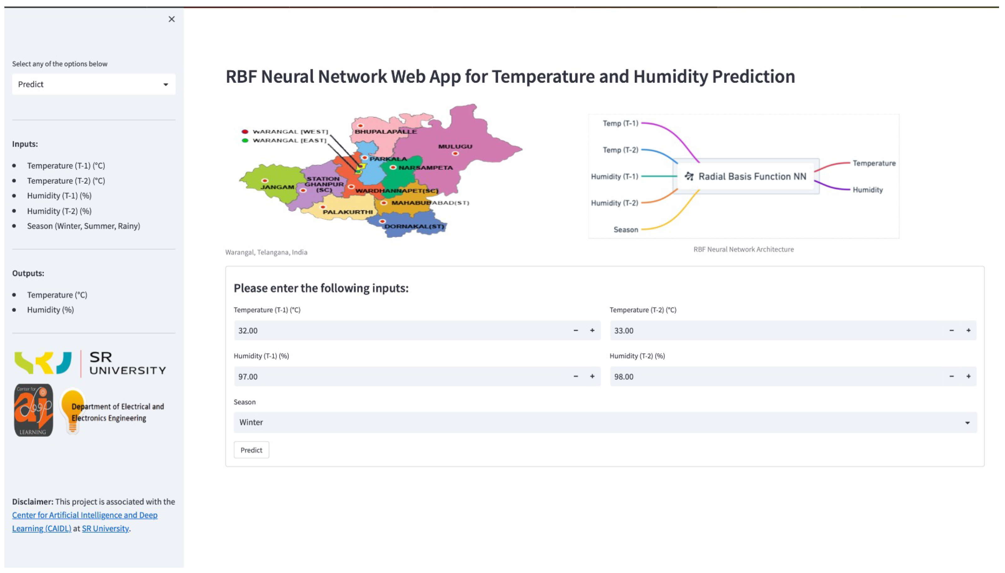
A web application was developed to enable temperature and humidity forecasting in the Warangal region. The application utilizes the RBFNN model in the backend. Figure 11 depicts the user interface of the web application. It can be accessed through the web link: https://sru-stlf-temp-humidity-rbf.streamlit.app/ (accessed on 12 March 2023).
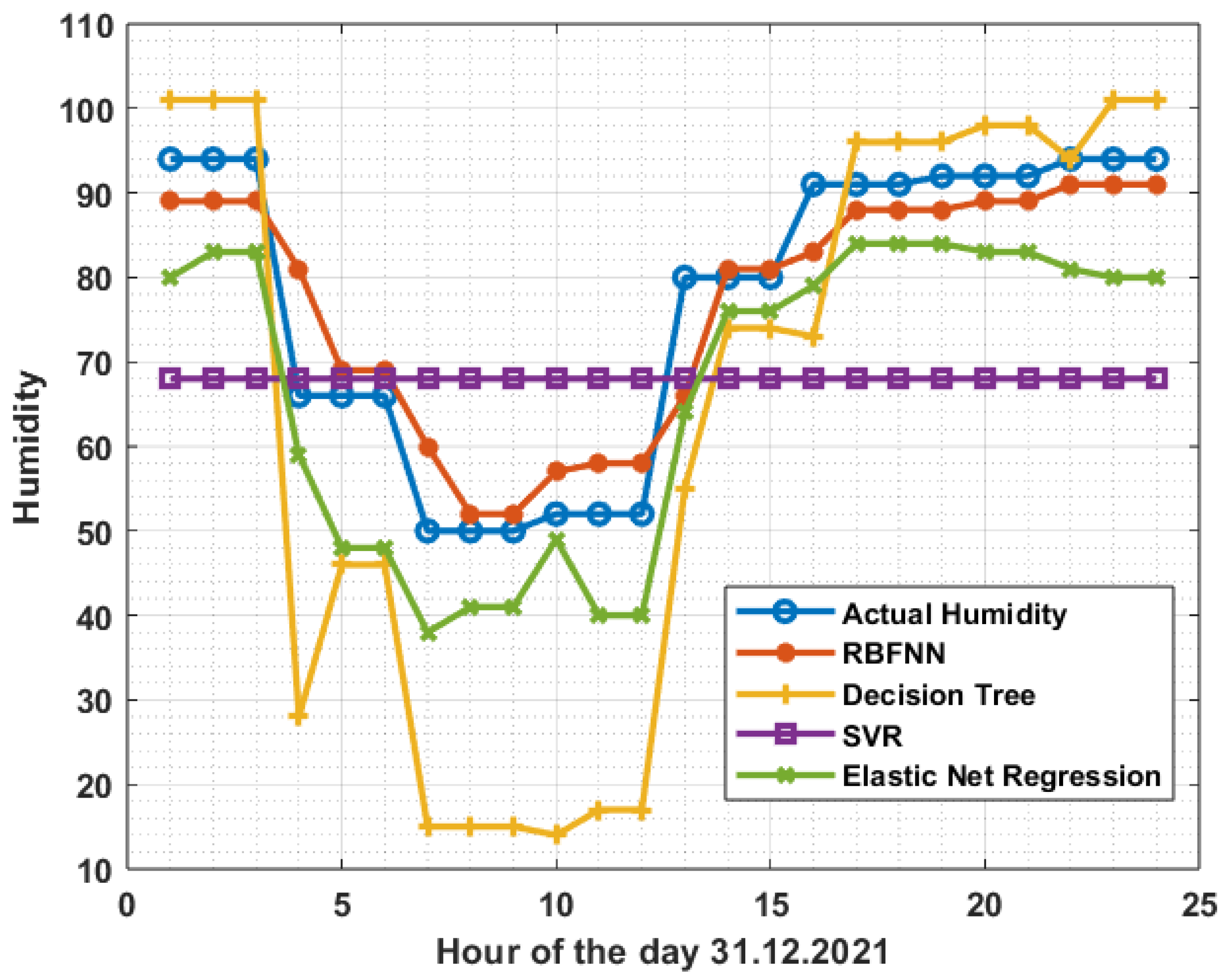
Temperature and humidity forecast obtained from different machine learning models, including the RBFNN, decision tree model [49], support vector regression [50], and elastic net regression [51], were compared with the corresponding actual values. As depicted in Figure 12 for temperature comparison and Figure 13 for humidity comparison, it can be observed that the forecast from the RBFNN model are closer to the actual values compared to the forecast from the other models.
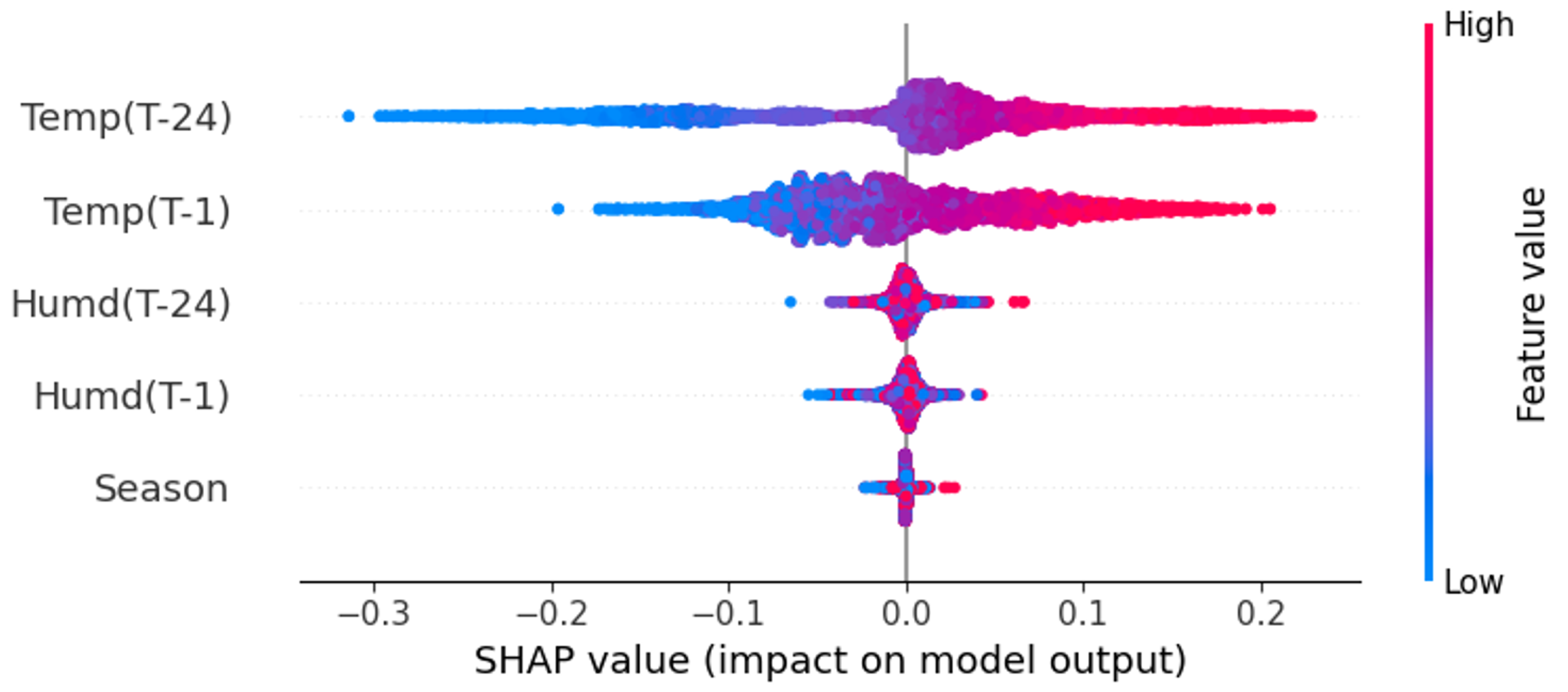
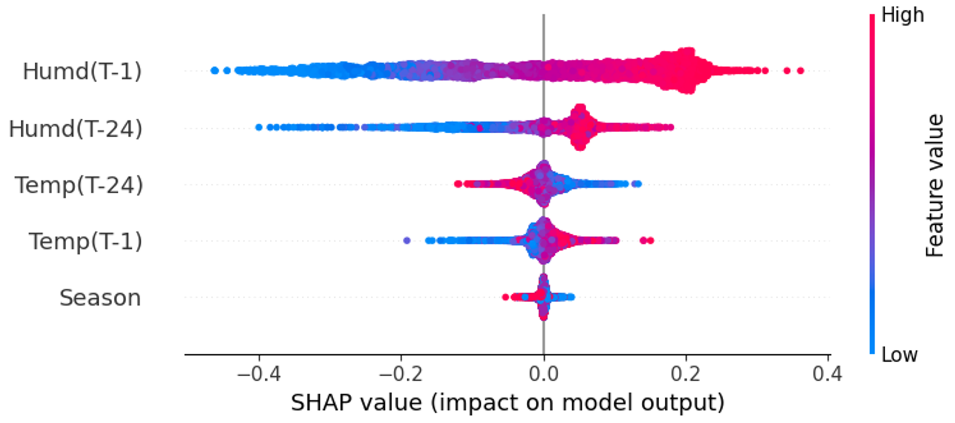
Model explainability, which demonstrates the impact of each feature on temperature forecasting and humidity forecasting, is presented in Table 10. From the table, it is observed that temperature data from one hour and one day before have a greater impact on temperature forecasting. Similarly, humidity data from one hour and one day before have a greater impact on humidity forecasting. The impact of various input features such as Temp(T-1), Temp(T-24), Humd(T-1), Humd(T-24), and season on temperature forecasting is shown in Figure 14. Similarly, the impact of various input features on humidity forecasting is shown in Figure 15.

5. Conclusions

In this study, an RBFNN model was developed to forecast weather (WX) conditions, specifically temperature and humidity, in Warangal, Telangana State, India. The objective of this research is to provide accurate forecasts for proper planning in the agriculture and electric sectors. The RBFNN model was trained and optimized by tuning the hyperparameters, including the number of centroids, width factor, and batch size.
After tuning, an optimal RBFNN model was identified for temperature forecasting, with 12 centroids, a width factor of 11, and a batch size of 32. This model achieves a validation loss of 0.0022. Similarly, for humidity forecasting, the optimal RBFNN model has 12 centroids, a width factor of 10, and a batch size of 128, with a validation loss of 0.0075.
To make the forecasting models accessible and user-friendly, a web application was developed. This application utilizes the optimized RBFNN models in the backend to forecast both temperature and humidity. The input features considered for the forecasts include temperature and humidity values from one hour and one day before, as well as the season.
Furthermore, this work can be extended by incorporating additional parameters such as air density, precipitation, and barometric pressure to enhance the forecasting accuracy and provide more comprehensive WX forecasts.

Author Contributions

Conceptualization, V.V., M.S. and P.K.; methodology, V.V. and P.K.; software, P.K.; validation, V.V. and S.R.S.; formal analysis, V.V. and M.S.; investigation, V.V.; resources, V.V. and P.K.; data curation, V.V. and P.K.; writing—original draft preparation, V.V.; writing—review and editing, V.V. and S.R.S.; visualization, P.K.; supervision, V.V.; project administration, V.V. All authors have read and agreed to the published version of the manuscript.

Funding

Woosong University’s Academic Research Funding—2023.

Data Availability Statement

The original active power load dataset used in this work and low dimensional representation of data developed from this work are available at https://data.mendeley.com/datasets/7vdt5rz47x/1 (accessed on 28 August 2022).

Conflicts of Interest

The authors declare no conflict of interest.

Abbreviations

The following abbreviations are used in this manuscript:
W h k Weights between output and latent space
b o Bias parameters at output layer
O k Output of output layer
n e t k Net input to output layer
O h Output of hidden layer
W h k n Weights connected to nth neuron in output layer
Δ W h k n Change in weights connected to nth neuron in output layer
Δ b 0 Change in bias connected to neurons in output layer
Temp(T-1)One-hour-ahead temperature from the time of forecasting
Temp(T-24)One-day-ahead temperature from the time of forecasting
Humd(T-1)One-hour-ahead humidity from the time of forecasting
Humd(T-24)One-day-ahead humidity from the time of forecasting
Temp(T)Temperature at time ‘T’
Humd(T)Humidity at time ‘T’
EDEuclidean distance
μ Mean vector at centroid
σ Standard deviation
RBFNNRadial basis function neural network
pWidth factor
C i Mean vector at centroid ‘i’
C j Mean vector at centroid ‘j’
η Learning rate
WXWeather
NWPNumerical weather prediction

Appendix A. Radial Basis Function Neural Network (RBFNN)

This section presents a step by step procedure for training the RBFNN and also explains how the trained RBFNN is used to forecast the temperature. The sample architecture of the RBFNN that is used in this section to explain the training and prediction procedure is shown in Figure A1.
Figure A1. Sample RBFNN architecture.
Urbansci 07 00068 g0a1
The initial weight matrix ( W h k ) is shown in Equation (A1). The bias parameter is 0.1, and the learning rate e t a = 0.1. The sample data that are used to explain the RBFNN training and prediction are shown in Table A1.
W h k = 0.1 0.2
Table A1. Sample data for temperature forecasting.
Temp(T-1)Temp(T-24)Humd(T-1)Humd(T-24)SeasonTemp
0.25860.25860.86360.86360.50.2586
0.48270.48270.38630.39770.50.4827
0.56890.56890.20450.22720.50.5689
0.51720.53440.27270.31810.50.5172
0.36200.36200.67040.82950.50.3620

Appendix A.1. Unsupervised Learning between Input and Hidden Layers

Two samples are randomly picked from the data as the mean vector for each centriod, i.e., m u 1 = [0.2586 0.2586 0.8636 0.8636 0.5] and μ 2 = [0.4827 0.4827 0.3863 0.3977 0.5 0.4827]. The euclidean distance between each sample and mean vector is calculated using Equation (5).
Iteration 1
Sample 1: X = [0.2586 0.2586 0.8636 0.8636 0.5 0.2586]
  • ED1 = ( ( 0.2586 0.2586 ) 2 + ( 0.2586 0.2586 ) 2 + ( 0.8636 0.8636 ) 2 + ( 0.8636 0.8636 ) 2 + ( 0.5 0.5 ) 2 ) = 0
  • ED2 = ( ( 0.2586 0.4827 ) 2 + ( 0.2586 0.4827 ) 2 + ( 0.8636 0.3863 ) 2 + ( 0.8636 0.3977 ) 2 + ( 0.5 0.5 ) 2 ) = 0.7384
Sample 2: X = [0.4827 0.4827 0.3863 0.3977 0.5 0.4827]
  • ED1 = ( ( 0.4827 0.2586 ) 2 + ( 0.4827 0.2586 ) 2 + ( 0.3863 0.8636 ) 2 + ( 0.3977 0.8636 ) 2 + ( 0.5 0.5 ) 2 ) = 0.73855
  • ED2 = ( ( 0.4827 0.4827 ) 2 + ( 0.4827 0.4827 ) 2 + ( 0.3863 0.3863 ) 2 + ( 0.3977 0.3977 ) 2 + ( 0.5 0.5 ) 2 ) = 0
Sample 3: X = [0.5689 0.5689 0.2045 0.2272 0.5 0.5689]
  • ED1 = ( ( 0.5689 0.2586 ) 2 + ( 0.5689 0.2586 ) 2 + ( 0.2045 0.8636 ) 2 + ( 0.2272 0.8636 ) 2 + ( 0.5 0.5 ) 2 ) = 1.0222
  • ED2 = ( ( 0.5689 0.4827 ) 2 + ( 0.5689 0.4827 ) 2 + ( 0.2045 0.3863 ) 2 + ( 0.2272 0.3977 ) 2 + ( 0.5 0.5 ) 2 ) = 0.27746
Sample 4: X = [0.5172 0.5344 0.2727 0.3181 0.5 0.5172]
  • ED1 = ( ( 0.5172 0.2586 ) 2 + ( 0.5344 0.2586 ) 2 + ( 0.2727 0.8636 ) 2 + ( 0.3181 0.8636 ) 2 + ( 0.5 0.5 ) 2 ) = 0.88864
  • ED2 = ( ( 0.5172 0.4827 ) 2 + ( 0.5344 0.4827 ) 2 + ( 0.2727 0.3863 ) 2 + ( 0.3181 0.3977 ) 2 + ( 0.5 0.5 ) 2 ) = 0.15102
Sample 5: X = [0.3620 0.3620 0.6704 0.8295 0.5 0.3620]
  • ED1 = ( ( 0.3620 0.2586 ) 2 + ( 0.3620 0.2586 ) 2 + ( 0.6704 0.8636 ) 2 + ( 0.8295 0.8636 ) 2 + ( 0.5 0.5 ) 2 ) = 0.24469
  • ED2 = ( ( 0.3620 0.4827 ) 2 + ( 0.3620 0.4827 ) 2 + ( 0.6704 0.3863 ) 2 + ( 0.8295 0.3977 ) 2 + ( 0.5 0.5 ) 2 ) = 0.54434
Iteration 2
Sample 1: X = [0.2586 0.2586 0.8636 0.8636 0.5 0.2586]
  • ED1 = ( ( 0.2586 0.3103 ) 2 + ( 0.2586 0.24162 ) 2 + ( 0.8636 0.767 ) 2 + ( 0.8636 0.8465 ) 2 + ( 0.5 0.5 ) 2 ) = 0.11218
  • ED2 = ( ( 0.2586 0.5229 ) 2 + ( 0.2586 0.5286 ) 2 + ( 0.8636 0.2878 ) 2 + ( 0.8636 0.3143 ) 2 + ( 0.5 0.5 ) 2 ) = 0.88093
Sample 2: X = [0.4827 0.4827 0.3863 0.3977 0.5 0.4827]
  • ED1 = ( ( 0.4827 0.3103 ) 2 + ( 0.4827 0.24162 ) 2 + ( 0.3863 0.767 ) 2 + ( 0.3977 0.8465 ) 2 + ( 0.5 0.5 ) 2 ) = 0.65893
  • ED2 = ( ( 0.4827 0.5229 ) 2 + ( 0.4827 0.5286 ) 2 + ( 0.3863 0.2878 ) 2 + ( 0.3977 0.3143 ) 2 + ( 0.5 0.5 ) 2 ) = 0.14276
Sample 3: X = [0.5689 0.5689 0.2045 0.2272 0.5 0.5689]
  • ED1 = ( ( 0.5689 0.3103 ) 2 + ( 0.5689 0.24162 ) 2 + ( 0.2045 0.767 ) 2 + ( 0.2272 0.8465 ) 2 + ( 0.5 0.5 ) 2 ) = 0.93484
  • ED2 = ( ( 0.5689 0.5229 ) 2 + ( 0.5689 0.5286 ) 2 + ( 0.2045 0.2878 ) 2 + ( 0.2272 0.3143 ) 2 + ( 0.5 0.5 ) 2 ) = 0.13515
Sample 4: X = [0.5172 0.5344 0.2727 0.3181 0.5 0.5172]
  • ED1 = ( ( 0.5172 0.3103 ) 2 + ( 0.5344 0.24162 ) 2 + ( 0.2727 0.767 ) 2 + ( 0.3181 0.8465 ) 2 + ( 0.5 0.5 ) 2 ) = 0.8075
  • ED2 = ( ( 0.5172 0.5229 ) 2 + ( 0.5344 0.5286 ) 2 + ( 0.2727 0.2878 ) 2 + ( 0.3181 0.3143 ) 2 + ( 0.5 0.5 ) 2 ) = 0.17566
Sample 5: X = [0.3620 0.3620 0.6704 0.8295 0.5 0.3620]
  • ED1 = ( ( 0.3620 0.3103 ) 2 + ( 0.3620 0.24162 ) 2 + ( 0.6704 0.767 ) 2 + ( 0.8295 0.8465 ) 2 + ( 0.5 0.5 ) 2 ) = 1.8443
  • ED2 = ( ( 0.3620 0.5229 ) 2 + ( 0.3620 0.5286 ) 2 + ( 0.6704 0.2878 ) 2 + ( 0.8295 0.3143 ) 2 + ( 0.5 0.5 ) 2 ) = 6.8224
From the calculations, it can be observed that sample 1 and sample 5 have minimum euclidean distance from centriod 1. Therefore, the mean vector for centriod 1 is updated as the mean of sample 1 and sample 5. Similarly, sample 2, sample 3, and sample 4 have minimum euclidean distance from centriod 2. Thus, the mean vector for centriod 2 is updated as the mean of sample 2, sample 3, and sample 4. The updated mean values of centriod 1 and centriod 2 are shown in Equation (A2) and Equation (A3), respectively.
μ 1 = 0.3103 0.3103 0.7670 0.8465 0.5
μ 2 = 0.5229 0.5286 0.2878 0.3144 0.5
Calculate the standard deviation ( Σ ) using Equation (6) for each centroid by considering width factor (P) as 2.
Standard deviation for centroid 1, i.e., σ 1
σ 1 = ( 1 2 [ ( 0.3103 0.5229 ) 2 + ( 0.3103 0.5286 ) 2 + ( 0.767 0.2878 ) 2 + ( 0.8465 0.3144 ) 2 + ( 0.5 0.5 ) 2 ] ) = 0.55
Standard deviation for centroid 2, i.e., σ 2
σ 2 = ( 1 2 [ ( 0.3103 0.5229 ) 2 + ( 0.3103 0.5286 ) 2 + ( 0.767 0.2878 ) 2 + ( 0.8465 0.3144 ) 2 + ( 0.5 0.5 ) 2 ] ) = 0.55
The output of first hidden neuron (h = 1) is calculated using Equation (7) as shown below.
sample 1: X = [0.2586 0.2586 0.8636 0.8636 0.5]
o 1 1 = e [ 0.2586 , 0.2586 , 0.8636 , 0.8636 , 0.5 ] [ 0.3103 , 0.3103 , 0.7670 , 0.8465 , 0.5 ] 2 2 × 0 . 55 2 = 0.9756
sample 2: X = [0.4827 0.4827 0.3863 0.3977 0.5]
o 2 1 = e [ 0.4827 , 0.4827 , 0.3863 , 0.3977 , 0.5 ] [ 0.3103 , 0.3103 , 0.7670 , 0.8465 , 0.5 ] 2 2 × 0 . 55 2 = 0.5113
sample 3: X = [0.5689 0.5689 0.2045 0.2272 0.5]
o 3 1 = e [ 0.5689 , 0.5689 , 0.2045 , 0.2272 , 0.5 ] [ 0.3103 , 0.3103 , 0.7670 , 0.8465 , 0.5 ] 2 2 × 0 . 55 2 = 0.2521
sample 4: X = [0.3103 0.3103 0.7670 0.8465 0.5]
o 4 1 = e [ 0.5172 , 0.5344 , 0.2727 , 0.3181 , 0.5 ] [ 0.3103 , 0.3103 , 0.7670 , 0.8465 , 0.5 ] 2 2 × 0 . 55 2 = 0.3609
sample 5: X = [0.3620 0.3620 0.6704 0.8295 0.5]
o 5 1 = e [ 0.3620 , 0.3620 , 0.6704 , 0.8295 , 0.5 ] [ 0.3103 , 0.3103 , 0.7670 , 0.8465 , 0.5 ] 2 2 × 0 . 55 2 = 0.9756
The output of second hidden neuron (h = 2) is calculated using Equation (7) as shown below.
sample 1: X = [0.2586 0.2586 0.8636 0.8636 0.5]
o 1 2 = e [ 0.2586 , 0.2586 , 0.8636 , 0.8636 , 0.5 ] [ 0.5229 , 0.5286 , 0.2878 , 0.3144 , 0.5 ] 2 2 × 0 . 55 2 = 0.2773
sample 2: X = [0.4827 0.4827 0.3863 0.3977 0.5]
o 2 2 = e [ 0.4827 , 0.4827 , 0.3863 , 0.3977 , 0.5 ] [ 0.5229 , 0.5286 , 0.2878 , 0.3144 , 0.5 ] 2 2 × 0 . 55 2 = 0.9669
sample 3: X = [0.5689 0.5689 0.2045 0.2272 0.5]
o 3 2 = e [ 0.5689 , 0.5689 , 0.2045 , 0.2272 , 0.5 ] [ 0.5229 , 0.5286 , 0.2878 , 0.3144 , 0.5 ] 2 2 × 0 . 55 2 = 0.9762
sample 4: X = [0.3103 0.3103 0.7670 0.8465 0.5]
o 4 2 = e [ 0.5172 , 0.5344 , 0.2727 , 0.3181 , 0.5 ] [ 0.5229 , 0.5286 , 0.2878 , 0.3144 , 0.5 ] 2 2 × 0 . 55 2 = 0.9995
sample 5: X = [0.3620 0.3620 0.6704 0.8295 0.5]
o 5 2 = e [ 0.3620 , 0.3620 , 0.6704 , 0.8295 , 0.5 ] [ 0.5229 , 0.5286 , 0.2878 , 0.3144 , 0.5 ] 2 2 × 0 . 55 2 = 0.4634
The final dataset that is used to update the weights( W h k ) and bias ( b k ) is shown in Table A2.
Table A2. Data used to update weights and bias between hidden layer and output layer.
Sample O 1 O 2 Temp
10.97560.27730.2586
20.51130.96690.4827
30.25210.97620.5689
40.36090.99950.5176
50.97560.46340.3620

Appendix A.2. Supervised Learning between Hidden and OUTPUT Layer

Iteration 1
Sample 1 = [0.9756 0.2773 0.2586]
  • The output of the RBFNN output layer is calculated using Equation (8)
o p = 0.1 0.2 × 0.9756 0.2773 + 0.1 = 0.1421
  • W h k is updated using Equation (9) and b k using (10)
W h k = 0.1 0.2 + 0.1 × ( 0.2586 0.1421 ) × 0.9756 0.2773 = 0.1114 0.1968
b k = 0.1 + 0.1 × ( 0.2586 0.1421 ) = 0.1117
Sample 2 = [0.5113 0.9669 0.4827]
  • The output of the RBFNN output layer is calculated using Equation (8)
o p = 0.1114 0.1968 × 0.5113 0.9669 + 0.1117 = 0.0217
  • W h k is updated using Equation (9) and b k using (10)
W h k = 0.1114 0.1968 + 0.1 × ( 0.4827 0.0217 ) × 0.5113 0.9669 = 0.1372 0.1480
b k = 0.1 + 0.1117 × ( 0.4827 + 0.0217 ) = 0.1621
Sample 3 = [0.2521 0.9762 0.5689]
  • The output of the RBFNN output layer is calculated using Equation (8)
o p = 0.1372 0.1480 × 0.2521 0.9762 + 0.1621 = 0.0531
  • W h k is updated using Equation (9) and b k using (10)
W h k = 0.1372 0.1480 + 0.1 × ( 0.5689 0.0531 ) × 0.2521 0.9762 = 0.1502 0.0980
b k = 0.1621 + 0.1 × ( 0.5689 + 0.0531 ) = 0.2137
Sample 4 = [0.3609 0.9995 0.5176]
  • The output of the RBFNN output layer is calculated using Equation (8)
o p = 0.1502 0.0980 × 0.3609 0.9995 + 0.2137 = 0.1700
  • W h k is updated using Equation (9) and b k using (10)
W h k = 0.1502 0.0980 + 0.1 × ( 0.5172 0.1700 ) × 0.3609 0.9995 = 0.1627 0.0632
b k = 0.2137 + 0.1 × ( 0.5172 + 0.1700 ) = 0.2484
Sample 5 = [0.9756 0.4634 0.3620]
  • The output of the RBFNN output layer is calculated using Equation (8)
o p = 0.1627 0.0632 × 0.9756 0.4634 + 0.2484 = 0.3778
  • W h k is updated using Equation (9) and b k using (10)
W h k = 0.1627 0.0632 + 0.1 × ( 0.3620 0.3778 ) × 0.9756 0.4634 = 0.1611 0.0640
b k = 0.2484 + 0.1 × ( 0.3620 + 0.3778 ) = 0.2468

Appendix B. Prediction Using Trained RBFNN

RBFNN was trained for one iteration with five samples. After training updated weights ( W h k ), bias ( b k ), centroids ( μ ), and standard deviation ( σ ) are shown below.
W h k = 0.1611 0.0640
b k = 0.2468
C e n t r o i d 1 = μ 1 = 0.3103 0.3103 0.7670 0.8465 0.5
C e n t r o i d 2 = μ 2 = 0.5229 0.5286 0.2878 0.3144 0.5
σ 1 = σ 2 = 0.55
The trained RBFNN predicts the output variable based on inputs {0.3620, 0.3620, 0.6704, 0.8295, 0.5} as shown below.
  • The output of each hidden neuron is calculated using centroids ( μ 1 ,   μ 2 ) and standard deviation ( σ 1 ,   σ 2 ) as shown below.
o 1 = e [ 0.3620 , 0.3620 , 0.6704 , 0.8295 , 0.5 ] [ 0.3103 , 0.3103 , 0.7670 , 0.8465 , 0.5 ] 2 2 × 0 . 55 2 = 0.3609
o 2 = e [ 0.3620 , 0.3620 , 0.6704 , 0.8295 , 0.5 ] [ 0.5229 , 0.5286 , 0.2878 , 0.3144 , 0.5 ] 2 2 × 0 . 55 2 = 0.4634
  • The output of the output neuron is calculated using weights ( W h k ), bias ( b k ), and output of hidden neurons as shown below.
o p = 0.1611 0.0640 × 0.9756 0.4634 + 0.2468 = 0.3743

References

  1. Abrego-Perez, A.L.; Pacheco-Carvajal, N.; Diaz-Jimenez, M.C. Forecasting Agricultural Financial Weather Risk Using PCA and SSA in an Index Insurance Model in Low-Income Economies. Appl. Sci. 2023, 13, 2425. [Google Scholar] [CrossRef]
  2. Shen, D.; Shi, W.F.; Tang, W.; Wang, Y.; Liao, J. The Agricultural Economic Value of Weather Forecasting in China. Sustainability 2022, 14, 17026. [Google Scholar] [CrossRef]
  3. Nyasulu, C.; Diattara, A.; Traore, A.; Deme, A.; Ba, C. Towards Resilient Agriculture to Hostile Climate Change in the Sahel Region: A Case Study of Machine Learning-Based Weather Prediction in Senegal. Agriculture 2022, 12, 1473. [Google Scholar] [CrossRef]
  4. Wang, D.; Cai, X. Irrigation scheduling—Role of weather forecasting and farmers’ behavior. J. Water Resour. Plan. Manag. 2009, 135, 364–372. [Google Scholar] [CrossRef]
  5. Ghate, V.P.; Miller, M.A.; DiPretore, L. Vertical velocity structure of marine boundary layer trade wind cumulus clouds. J. Geophys. Res. Atmos. 2011, 116. [Google Scholar] [CrossRef] [Green Version]
  6. Leu, J.S.; Su, K.W.; Chen, C.T. Ambient mesoscale weather forecasting system featuring mobile augmented reality. Multimed. Tools Appl. 2014, 72, 1585–1609. [Google Scholar] [CrossRef]
  7. Wang, T.; Zhang, Y.; Zhi, X.; Ji, Y. Multi-Model Ensemble Forecasts of Surface Air Temperatures in Henan Province Based on Machine Learning. Atmosphere 2023, 14, 520. [Google Scholar] [CrossRef]
  8. Zhang, L.; Zhao, X.; Ge, J.; Zhang, J.; Traore, S.; Fipps, G.; Luo, Y. Evaluation of Five Equations for Short-Term Reference Evapotranspiration Forecasting Using Public Temperature Forecasts for North China Plain. Water 2022, 14, 2888. [Google Scholar] [CrossRef]
  9. Lee, Y.; Choi, D.; Jung, Y.; Ko, M. Application of Technology to Develop a Framework for Predicting Power Output of a PV System Based on a Spatial Interpolation Technique: A Case Study in South Korea. Energies 2022, 15, 8755. [Google Scholar] [CrossRef]
  10. Sigauke, C.; Chandiwana, E.; Bere, A. Spatio-Temporal Forecasting of Global Horizontal Irradiance Using Bayesian Inference. Appl. Sci. 2023, 13, 201. [Google Scholar] [CrossRef]
  11. Wang, S.; Dai, T.; Li, C.; Cheng, Y.; Huang, G.; Shi, G. Improving Clear-Sky Solar Power Prediction over China by Assimilating Himawari-8 Aerosol Optical Depth with WRF-Chem-Solar. Remote Sens. 2022, 14, 4990. [Google Scholar] [CrossRef]
  12. Jeon, H.J.; Choi, M.W.; Lee, O.J. Day-Ahead Hourly Solar Irradiance Forecasting Based on Multi-Attributed Spatio-Temporal Graph Convolutional Network. Sensors 2022, 22, 7179. [Google Scholar] [CrossRef]
  13. Alkhayat, G.; Hasan, S.H.; Mehmood, R. SENERGY: A Novel Deep Learning-Based Auto-Selective Approach and Tool for Solar Energy Forecasting. Energies 2022, 15, 6659. [Google Scholar] [CrossRef]
  14. Tu, C.S.; Tsai, W.C.; Hong, C.M.; Lin, W.M. Short-Term Solar Power Forecasting via General Regression Neural Network with Grey Wolf Optimization. Energies 2022, 15, 6624. [Google Scholar] [CrossRef]
  15. Xin, J.; Bao, D.; Ma, Y.; Ma, Y.; Gong, C.; Qiao, S.; Jiang, Y.; Ren, X.; Pang, T.; Yan, P. Forecasting and Optimization of Wind Speed over the Gobi Grassland Wind Farm in Western Inner Mongolia. Atmosphere 2022, 13, 1943. [Google Scholar] [CrossRef]
  16. Lyu, Y.; Zhi, X.; Wu, H.; Zhou, H.; Kong, D.; Zhu, S.; Zhang, Y.; Hao, C. Analyses on the Multimodel Wind Forecasts and Error Decompositions over North China. Atmosphere 2022, 13, 1652. [Google Scholar] [CrossRef]
  17. Rubin, Y.; Sohn, S.; Alpert, P. High-Resolution Humidity Observations Based on Commercial Microwave Links (CML) Data—Case of Tel Aviv Metropolitan Area. Remote Sens. 2023, 15, 345. [Google Scholar] [CrossRef]
  18. Cai, C.; Wang, J.; Li, Z.; Shen, X.; Wen, J.; Wang, H.; Wu, C. A New Hybrid Framework for Error Correction and Uncertainty Analysis of Precipitation Forecasts with Combined Postprocessors. Water 2022, 14, 3072. [Google Scholar] [CrossRef]
  19. Fathi, M.; Haghi Kashani, M.; Jameii, S.M.; Mahdipour, E. Big data analytics in weather forecasting: A systematic review. Arch. Comput. Methods Eng. 2022, 29, 1247–1275. [Google Scholar] [CrossRef]
  20. Chung, C.Y.C.; Kumar, V.R. Knowledge acquisition using a neural network for a weather forecasting knowledge-based system. Neural Comput. Appl. 1993, 1, 215–223. [Google Scholar] [CrossRef]
  21. Pandey, A.; Agrawal, C.; Agrawal, M. A hadoop based weather prediction model for classification of weather data. In Proceedings of the 2017 Second International Conference on Electrical, Computer and Communication Technologies (ICECCT), Coimbatore, Tamil Nadu, India, 22–24 February 2017; IEEE: New York, NY, USA, 2017; pp. 1–5. [Google Scholar]
  22. Zhao, X.; Sun, Q.; Lin, X. Physical Attention-Gated Spatial-Temporal Predictive Network for Weather Forecasting. Mathematics 2023, 11, 1330. [Google Scholar] [CrossRef]
  23. Bauer, P.; Thorpe, A.; Brunet, G. The quiet revolution of numerical weather prediction. Nature 2015, 525, 47–55. [Google Scholar] [CrossRef] [PubMed]
  24. de Mourgues, M.; Emde, C.; Mayer, B. Optimized Wavelength Sampling for Thermal Radiative Transfer in Numerical Weather Prediction Models. Atmosphere 2023, 14, 332. [Google Scholar] [CrossRef]
  25. Qin, Y.; Liu, Y.; Jiang, X.; Yang, L.; Xu, H.; Shi, Y.; Huo, Z. Grid-to-Point Deep-Learning Error Correction for the Surface Weather Forecasts of a Fine-Scale Numerical Weather Prediction System. Atmosphere 2023, 14, 145. [Google Scholar] [CrossRef]
  26. Holmstrom, M.; Liu, D.; Vo, C. Machine learning applied to weather forecasting. Meteorol. Appl. 2016, 10, 1–5. [Google Scholar]
  27. Abuella, M.; Chowdhury, B. Solar power probabilistic forecasting by using multiple linear regression analysis. In Proceedings of the SoutheastCon 2015, Fort Lauderdale, FL, USA, 9–12 April 2015; pp. 1–5. [Google Scholar] [CrossRef]
  28. Sharma, N.; Sharma, P.; Irwin, D.; Shenoy, P. Predicting solar generation from weather forecasts using machine learning. In Proceedings of the 2011 IEEE International Conference on Smart Grid Communications (SmartGridComm), Brussels, Belgium, 17–20 October 2011; IEEE: New York, NY, USA, 2011; pp. 528–533. [Google Scholar]
  29. Kuligowski, R.J.; Barros, A.P. Localized precipitation forecasts from a numerical weather prediction model using artificial neural networks. Weather Forecast. 1998, 13, 1194–1204. [Google Scholar] [CrossRef]
  30. Li, Y.; Lang, J.; Ji, L.; Zhong, J.; Wang, Z.; Guo, Y.; He, S. Weather forecasting using ensemble of spatial-temporal attention network and multi-layer perceptron. Asia-Pac. J. Atmos. Sci. 2021, 57, 533–546. [Google Scholar] [CrossRef]
  31. Tektaş, M. Weather forecasting using ANFIS and ARIMA models. Environ. Res. Eng. Manag. 2010, 51, 5–10. [Google Scholar]
  32. Hewage, P.; Behera, A.; Trovati, M.; Pereira, E.; Ghahremani, M.; Palmieri, F.; Liu, Y. Temporal convolutional neural (TCN) network for an effective weather forecasting using time-series data from the local weather station. Soft Comput. 2020, 24, 16453–16482. [Google Scholar] [CrossRef] [Green Version]
  33. Hossain, M.S.; Mahmood, H. Short-Term Photovoltaic Power Forecasting Using an LSTM Neural Network and Synthetic Weather Forecast. IEEE Access 2020, 8, 172524–172533. [Google Scholar] [CrossRef]
  34. Lee, C.C.; Chung, P.C.; Tsai, J.R.; Chang, C.I. Robust radial basis function neural networks. IEEE Trans. Syst. Man Cybern. Part B (Cybern.) 1999, 29, 674–685. [Google Scholar]
  35. Tang, X.; Xu, B.; Xu, Z. Reactor Temperature Prediction Method Based on CPSO-RBF-BP Neural Network. Appl. Sci. 2023, 13, 3230. [Google Scholar] [CrossRef]
  36. Wang, W.; Jing, Z.; Zhao, S.; Lu, Z.; Xing, Z.; Guo, S. Intelligent Height Adjustment Method of Shearer Drum Based on Rough Set Significance Reduction and Fuzzy Rough Radial Basis Function Neural Network. Appl. Sci. 2023, 13, 2877. [Google Scholar] [CrossRef]
  37. Yang, P.; Wang, T.; Yang, H.; Meng, C.; Zhang, H.; Cheng, L. The Performance of Electronic Current Transformer Fault Diagnosis Model: Using an Improved Whale Optimization Algorithm and RBF Neural Network. Electronics 2023, 12, 1066. [Google Scholar] [CrossRef]
  38. Veeramsetty, V.; Edudodla, B.R.; Salkuti, S.R. Zero-Crossing Point Detection of Sinusoidal Signal in Presence of Noise and Harmonics Using Deep Neural Networks. Algorithms 2021, 14, 329. [Google Scholar] [CrossRef]
  39. Veeramsetty, V.; Deshmukh, R. Electric power load forecasting on a 33/11 kV substation using artificial neural networks. SN Appl. Sci. 2020, 2, 855. [Google Scholar] [CrossRef] [Green Version]
  40. Tsoulos, I.G.; Charilogis, V. Locating the Parameters of RBF Networks Using a Hybrid Particle Swarm Optimization Method. Algorithms 2023, 16, 71. [Google Scholar] [CrossRef]
  41. Chen, H.; Liang, Y.; Huang, H.; Huang, Q.; Gu, W.; Liang, H. Live Pig-Weight Learning and Prediction Method Based on a Multilayer RBF Network. Agriculture 2023, 13, 253. [Google Scholar] [CrossRef]
  42. Alzaeemi, S.A.; Noman, E.A.; Al-shaibani, M.M.; Al-Gheethi, A.; Mohamed, R.M.S.R.; Almoheer, R.; Seif, M.; Tay, K.G.; Zin, N.M.; El Enshasy, H.A. Improvement of L-asparaginase, an Anticancer Agent of Aspergillus arenarioides EAN603 in Submerged Fermentation Using a Radial Basis Function Neural Network with a Specific Genetic Algorithm (RBFNN-GA). Fermentation 2023, 9, 200. [Google Scholar] [CrossRef]
  43. Veeramsetty, V.; Rakesh Chandra, D.; Salkuti, S.R. Short Term Active Power Load Forecasting Using Machine Learning with Feature Selection. In Next Generation Smart Grids: Modeling, Control and Optimization; Springer: Berlin/Heidelberg, Germany, 2022; pp. 103–124. [Google Scholar]
  44. Venkataramana, V.; Pravallika, J.; Eslavath, R.; Srividya, S.; Surender Reddy, S. A Platform Independent Web-Application for Short-Term Electric Power Load Forecasting on a 33/11 kV Substation Using Regression Model. Adv. Electr. Electron. Eng. 2023, 20, 432–443. [Google Scholar]
  45. Veeramsetty, V.; Chandra, D.R.; Salkuti, S.R. Short-term electric power load forecasting using factor analysis and long short-term memory for smart cities. Int. J. Circuit Theory Appl. 2021, 49, 1678–1703. [Google Scholar] [CrossRef]
  46. Veeramsetty, V.; Reddy, K.R.; Santhosh, M.; Mohnot, A.; Singal, G. Short-term electric power load forecasting using random forest and gated recurrent unit. Electr. Eng. 2022, 104, 307–329. [Google Scholar] [CrossRef]
  47. Veeramsetty, V.; Chandra, D.R.; Grimaccia, F.; Mussetta, M. Short term electric power load forecasting using principal component analysis and recurrent neural networks. Forecasting 2022, 4, 149–164. [Google Scholar] [CrossRef]
  48. Veeramsetty, V.; Mohnot, A.; Singal, G.; Salkuti, S.R. Short term active power load prediction on a 33/11 kv substation using regression models. Energies 2021, 14, 2981. [Google Scholar] [CrossRef]
  49. Veeramsetty, V.; Sai Pavan Kumar, M.; Salkuti, S.R. Platform-Independent Web Application for Short-Term Electric Power Load Forecasting on 33/11 kV Substation Using Regression Tree. Computers 2022, 11, 119. [Google Scholar] [CrossRef]
  50. Smola, A.J.; Schölkopf, B. A tutorial on support vector regression. Stat. Comput. 2004, 14, 199–222. [Google Scholar] [CrossRef] [Green Version]
  51. Hans, C. Elastic net regression modeling with the orthant normal prior. J. Am. Stat. Assoc. 2011, 106, 1383–1393. [Google Scholar] [CrossRef]
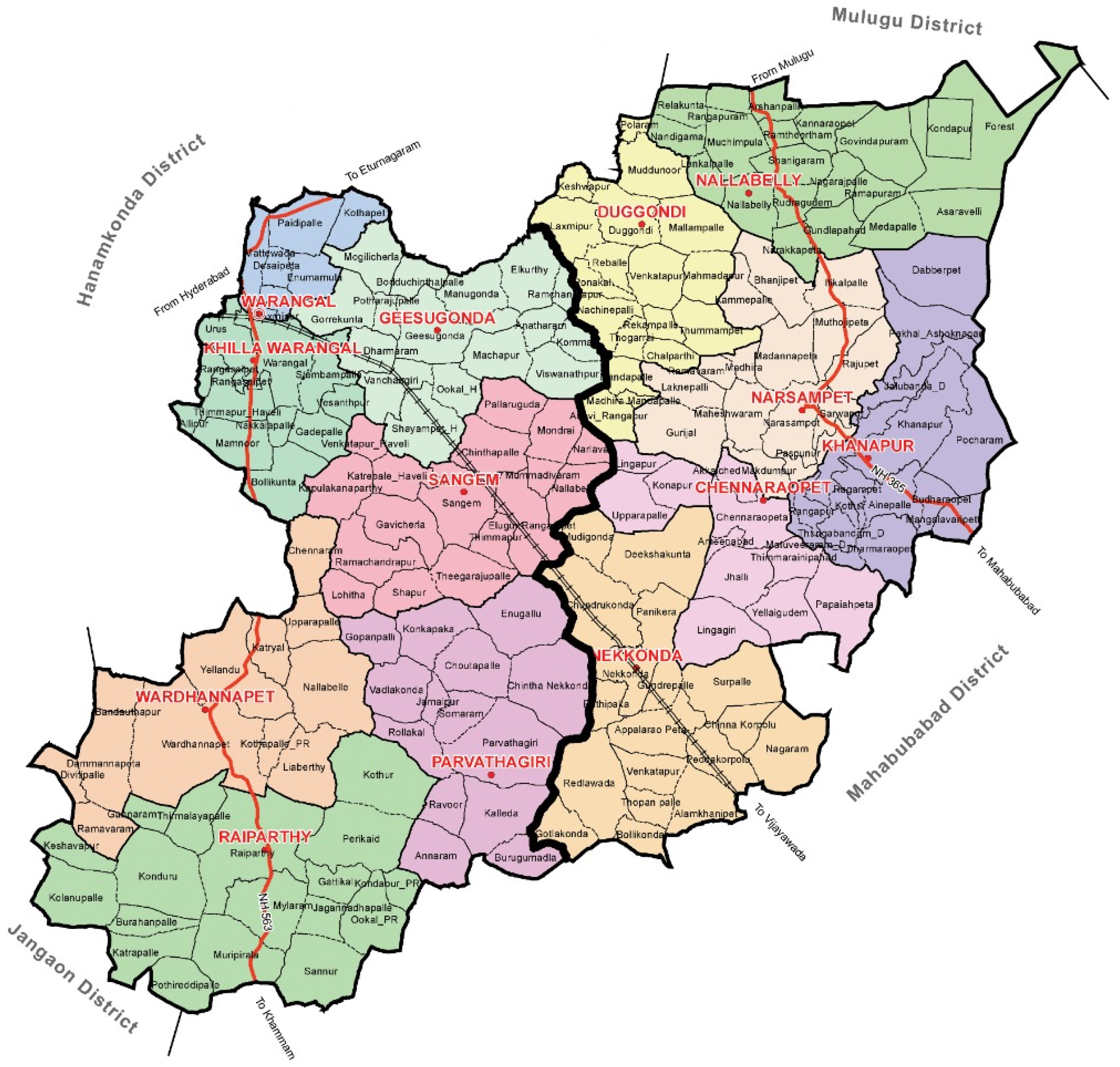
Figure 1. Warangal district map (https://warangal.telangana.gov.in/map-of-district/ (accessed on 12 March 2023)).
Urbansci 07 00068 g001
Figure 2. Box plot for temperature dataset.
Urbansci 07 00068 g002
Figure 3. Average temperature over the year.
Urbansci 07 00068 g003
Figure 4. Box plot for humidity dataset.
Urbansci 07 00068 g004
Figure 5. RBFNN architecture for temperature forecasting.
Urbansci 07 00068 g005
Figure 6. RBFNN architecture for humidity forecasting.
Urbansci 07 00068 g006
Figure 7. Converging characteristics of RBFNN for temperature forecasting.
Urbansci 07 00068 g007
Figure 8. Converging characteristics of RBFNN for humidity forecasting.
Urbansci 07 00068 g008
Figure 9. RBFNN model validation for temperature forecasting.
Urbansci 07 00068 g009
Figure 10. RBFNN model validation for humidity forecasting.
Urbansci 07 00068 g010
Figure 11. Web application for temperature and humidity forecasting.
Urbansci 07 00068 g011
Figure 12. Comparison of hourly temperature forecast on 31 December 2021.
Urbansci 07 00068 g012
Figure 13. Comparison of hourly humidity forecast on 31 December 2021.
Urbansci 07 00068 g013
Figure 14. Impact of input features on temperature forecasting.
Urbansci 07 00068 g014
Figure 15. Impact of input features on humidity forecasting.
Urbansci 07 00068 g015
Table 1. Five samples from temperature dataset.
Temp(T-1)Temp(T-24)Humd(T-1)Humd(T-24)SeasonTemp(T)
62658990165
65789049178
78834834183
83813242180
71677387167
Table 2. Statistical information from temperature dataset.
ParameterTemp(T-1)Temp(T-24)Humd(T-1)Humd(T-24)SeasonTemp(T)
count873687368736873687368736
mean81816868181
std99212119
min50501414050
25%77775252077
50%81817272181
75%86868787286
max1081081021022108
Table 3. Five samples from humidity dataset.
Temp(T-1)Temp(T-24)Humd(T-1)Humd(T-24)SeasonHumd(T)
62658990190
65789049148
88787390273
81828470070
78849177091
Table 4. Statistical information from humidity dataset.
ParameterTemp(T-1)Temp(T-24)Humd(T-1)Humd(T-24)SeasonHumd(T)
count873687368736873687368736
mean81816868168
std992121121
min50501414014
25%77775252052
50%81817272172
75%86868787287
max1081081021022102
Table 5. Missing value information.
ColumnNo. of Missing Values
Temp(T-1)0
Temp(T-24)0
Humd(T-1)0
Humd(T-24)0
Season0
T0
Humd(H)0
Table 6. RBFNN training loss for temperature forecast.
Width Factor
Centroids23456789101112
40.00850.00740.0064--------
60.00670.00570.00520.00460.0038------
80.00720.00650.00490.00410.00380.00400.0032----
100.00790.00580.00550.00470.00370.00420.00380.00360.0032--
120.00780.00590.00500.00420.00400.00380.00390.00370.00440.00370.0039
Table 7. RBFNN validation loss for temperature forecast.
Centroids23456789101112
40.00820.01050.0057--------
60.00660.00530.00440.00340.0032------
80.00810.00770.00650.00330.00340.00430.0109----
100.00810.00490.00790.00790.00460.00790.00640.00320.0026--
120.00750.00430.00340.00370.00390.00370.00240.00310.00240.00220.0028
Table 8. RBFNN training loss for humidity forecast.
 Width Factor
Centroids2345678910
40.016850.013760.0112------
60.012720.01190.01090.011580.0101----
80.01370.01180.01020.011210.010.01100.01--
100.01370.0120.0120.0110.01120.01060.01080.01160.01
120.013810.010610.01100.010510.00990.01180.010.010.011
Table 9. RBFNN validation loss for humidity forecast.
 Width Factor
Centroids2345678910
40.01650.01220.0105------
60.01220.01390.01000.01120.0083----
80.01340.01000.00980.00880.01120.00950.0082--
100.01880.00990.00980.00860.00860.01640.00870.00830.0083
120.01360.01350.01110.00900.01230.00950.00960.00840.0078
Table 10. RBFNN model explainability for temperature forecast.
Weightage of Feature
FeatureTemperature ForecastingHumidity Forecasting
Temp(T-24)0.6090 +/− 0.03610.0319 +/− 0.0034
Temp(T-1)0.3438 +/− 0.03580.0344 +/− 0.0048
Humd(T-24)0.0239 +/− 0.00270.1512 +/− 0.0610
Humd(T-1)0.0200 +/− 0.00210.7757 +/− 0.0598
Season0.0033 +/− 0.00180.0068 +/− 0.0025
Disclaimer/Publisher’s Note: The statements, opinions and data contained in all publications are solely those of the individual author(s) and contributor(s) and not of MDPI and/or the editor(s). MDPI and/or the editor(s) disclaim responsibility for any injury to people or property resulting from any ideas, methods, instructions or products referred to in the content.