Influence of Near-Surface Air Temperature on Atmospheric Correction Factor for Internal Combustion Engines During Mobile Transects in an Extreme Arid City of Northwestern Mexico

Abstract

This study investigates the influence of near-surface air temperature on the performance of internal combustion engines during mobile transects conducted in Mexicali, Baja California, Mexico, one of the hottest cities in North America. Field measurements were carried out along a 15 km urban transect on representative days in April, August, and February. Air temperature and relative humidity were recorded simultaneously at two engine air intake heights (0.66 m and 2.5 m), complemented by surface temperature data obtained from both in situ measurements and Landsat 8 thermal imagery. The results indicate that near-surface air temperature exhibits considerable spatial and temporal variability and is closely associated with land surface temperature (LST) patterns derived from satellite observations. The correction factor (Cf), used to quantify the combined effects of air temperature and atmospheric pressure on engine performance, showed that extremely high temperatures (approaching 50 °C) may reduce engine performance by up to 3.35% relative to standard test conditions. Conversely, cooler winter conditions may improve engine performance by approximately 4.6%. These results suggest that vehicle operation under extremely hot climatic conditions may deviate from the standardized assumptions adopted by the Intergovernmental Panel on Climate Change (IPCC) for emission factor estimation. This study contributes to a better understanding of the effects of extreme urban heat on vehicle performance and demonstrates that localized thermal conditions may influence the assumptions commonly used in vehicle emission assessments. The findings provide valuable information for improving greenhouse gas emission inventories and support evidence-based climate adaptation and urban planning strategies in arid cities.

1. Introduction

Variations in atmospheric conditions have been shown to cause discrepancies between the actual power output of internal combustion engines and their rated specifications, primarily due to changes in ambient pressure, temperature, and humidity that affect air intake and combustion processes [1]. Furthermore, the influence of intake air temperature on engine operation and performance has been extensively documented [2,3]. Several studies have demonstrated that variations in intake air temperature can significantly affect engine power output and fuel consumption in passenger vehicles [3,4]. In addition, extreme ambient temperatures have been shown to influence vehicle energy consumption, fuel use, and CO₂ emissions under real-world driving conditions [5,6]. Such variations in atmospheric conditions may arise from temperature differences between urban areas and their surrounding rural environments. When urban areas are warmer than adjacent rural regions, the Urban Heat Island (UHI) effect develops and may consequently influence engine performance [7]. Anthropogenic activities also contribute to the formation of distinct urban microclimates. For example, previous studies have identified characteristic thermal patterns in urban, suburban, and rural environments [8,9].

Table 1. Scientific methods commonly used to analyze temperature variations across urban, suburban, and rural environments.

Method	Thermal Index/Variable	Typical Findings	Limitations and Shortcomings
Fixed meteorological station network [10,11]	Air Temperature (Ta), Relative Humidity (RH), Heat Index (HI)	Detects spatial and temporal variations in air temperature, urban heat island (UHI) intensity, and long-term climatic trends. Urban centers are generally warmer than surrounding suburban and rural areas.	Limited spatial representativeness; installation and maintenance costs; may not adequately capture local microclimatic variability.
Satellite Remote Sensing [12,13]	Land Surface Temperature (LST), Surface Urban Heat Island (SUHI)	Reveals relationships between urbanization, vegetation cover, and land surface heating. Impervious surfaces consistently exhibit higher temperatures than vegetated areas.	Retrieves land surface temperature (LST) rather than near-surface air temperature; affected by cloud cover and satellite overpass timing.
GIS Spatial Analysis and Interpolation [14,15]	Interpolated Temperature Surfaces, Thermal Hotspots	Produces continuous temperature maps and identifies thermal hotspots and cool spots.	Results depend on sensor density and interpolation method; uncertainty increases in poorly sampled areas.
Urban Climate Modeling [16,17]	Air Temperature (Ta), Mean Radiant Temperature (MRT), Surface Energy Balance	Simulates present and future urban climates and evaluates mitigation strategies such as green roofs, urban trees, and reflective surfaces.	Requires extensive input data, calibration, and computational resources; results depend on model assumptions.
Dense Sensor Networks (IoT) [18,19]	Ta, RH, Heat Index, Wet-Bulb Temperature	Provides high-resolution, real-time observations and high-density observations of urban thermal variability and heat exposure.	Measurement quality depends on sensor accuracy and calibration; large datasets require quality-control procedures.
Local Climate Zone (LCZ) Analysis [11,20]	LCZ-based Temperature Differences, UHII	Characterizes the influence of urban morphology on local thermal conditions. Compact high-density zones are typically warmer than open or vegetated areas.	Subject to classification uncertainties; Does not directly measure air or surface temperature.
Micrometeorological Flux Measurements [21,22]	Sensible Heat Flux, Latent Heat Flux, Surface Energy Balance	Quantifies physical mechanisms controlling urban heat storage and energy exchange.	Requires specialized instrumentation and has limited spatial representativeness.
Human Thermal Comfort Assessment [23,24]	UTCI, PET, WBGT, MRT	Evaluates thermal stress experienced by urban populations and identifies areas and periods of elevated thermal stress.	Requires multiple meteorological inputs and, in some cases, assumptions regarding human physiology and activity.

summarizes the principal research methods that have been used to investigate these thermal variations.

These areas are interconnected by different types of roads that support the daily movement of vehicles with diverse operating characteristics. Therefore, it is essential to investigate the urban microclimate and its spatial heterogeneity along the vehicular corridors that connect different parts of a city. Such investigations should consider both the causes and the consequences of spatial and temporal temperature variations, which are influenced by local urban morphology, anthropogenic activities, urban planning, and transient meteorological conditions [25,26]. Understanding the physical characteristics of the urban environment has motivated an increasing number of studies based on mobile measurements. This objective can be achieved by identifying representative mobile transects through field observations and by developing models that integrate data from reference weather stations with measurements collected along mobile transects [26,27,28,29,30,31,32].

Mobile air temperature monitoring has emerged as an effective approach for characterizing fine-scale thermal variability across urban areas. In most cases, mobile measurements reveal greater spatial variability and higher temperature values than those recorded simultaneously at fixed monitoring stations. Microscale observations have demonstrated that fixed stations are often insufficient to capture the thermal variability of adjacent streetscapes. Consequently, mobile air temperature monitoring provides a valuable tool for obtaining high-resolution spatial and temporal temperature data within urban environments [33]. The main advantages of the mobile transect method are summarized in

Table 2. Main advantages of the mobile transect method relative to other methods used to characterize urban temperature variability.

Advantage	Main Characteristics
Very high spatial resolution [11,34]	A single traverse can collect measurements every few meters, revealing street-by-street temperature differences that may not be captured by fixed stations, flux towers, or conventional sensor networks.
Cost-effectiveness [35,36]	Requires only a limited number of calibrated sensors mounted on a vehicle, bicycle, or carried by an operator, making it much less expensive than establishing dense meteorological networks or flux towers.
Direct measurement of air temperature [12,13]	Unlike satellite remote sensing, which measures Land Surface Temperature (LST), mobile transects measure the near-surface air temperature experienced at pedestrian level.
Rapid spatial coverage [12,37]	Large portions of a city can be surveyed within a short period (e.g., 1–3 h), allowing the characterization of different urban environments under similar weather conditions.
Identification of microclimates [10,38]	Particularly useful for detecting thermal differences associated with parks, water bodies, street canyons, industrial areas, commercial districts, and residential neighborhoods.
Flexibility [36,39]	Survey routes can be modified easily to target specific areas of interest without installing permanent infrastructure.
Suitable for Urban Heat Island studies [10,11]	Widely used to characterize urban heat island intensity and intra-urban thermal patterns.
Useful for validating other datasets [12,13,36]	Frequently used to validate satellite-derived LST products, GIS-based interpolation results, and urban climate model simulations.

.

The interaction between near-surface air temperature and internal combustion engine performance is direct, as intake air properties influence the combustion process. Near-surface air masses are strongly affected by heat transfer from road surfaces and other urban materials; therefore, analyzing the thermal behavior at the land–atmosphere interface within the study area is essential. One effective approach for this purpose is satellite remote sensing through thermal image processing. Thermal imagery is widely used to identify urban thermal hotspots based on the assumption that spatial patterns of LST are generally associated with corresponding patterns of near-surface air temperature [40]. Furthermore, land use and land cover (LULC) influence variables such as the normalized difference vegetation index (NDVI), surface emissivity, albedo, evapotranspiration, the Bowen ratio, and atmospheric correction procedures, all of which contribute to the accurate retrieval of land surface temperature from satellite imagery [41,42,43,44,45]. The accuracy of these estimates depends on the urban and rural characteristics of the study area.

Vehicular dynamics are also closely related to the measurement and estimation of pollutant emissions and emission factors for both roadways and vehicles. These parameters may be influenced directly or indirectly by air temperature, particularly in arid regions where extreme thermal conditions affect both vehicle operation and the dispersion of pollutants. For example, a study conducted in the U.S.–Mexico border region, encompassing El Paso, Texas, and Ciudad Juárez, Mexico, estimated particulate matter (PM₁₀) emission factors from unpaved roads by considering variables such as vehicle speed and accumulated soil loss [46]. Similarly, in Doha, Qatar, researchers measured PM₁₀ and PM₂.₅ concentrations near a heavily trafficked roadway and combined these measurements with environmental variables, including air temperature, wind speed, relative humidity, road surface characteristics, and particulate source areas, to develop regression models for estimating vehicular emission factors [47].

In a separate study conducted in the border region between Mexicali, Baja California, Mexico, and Calexico, California, USA, vehicular CO₂ emissions were estimated before and during the COVID-19 pandemic. Although the emission factors were based on the IPCC guidelines, which do not account for local variations in air temperature, the incorporation of activity data and cross-border vehicle counts enabled a more detailed characterization of vehicular emissions in the study area [48].

In the aforementioned studies, vehicular activity was shown to have a substantial influence on air quality. Therefore, it is important to quantify the effects of atmospheric conditions on internal combustion engine performance. Vehicle manufacturers establish standardized reference conditions, including air temperature and atmospheric pressure, to evaluate engine performance under controlled testing conditions. However, in arid regions that experience extreme heat, actual atmospheric conditions may differ substantially from these standardized conditions, particularly with respect to air temperature, potentially affecting engine performance. Despite the widespread use of standard correction factors to evaluate internal combustion engine performance under standardized testing conditions, limited attention has been given to the applicability of these factors under extreme urban climatic conditions and to their implications for emission estimation. Therefore, this study aims to quantify the influence of air temperature and atmospheric pressure on the theoretical correction factor (Cf), which is used to account for the effects of atmospheric conditions on engine performance, using representative conditions observed during April, August, and February. Mobile transects were conducted to measure near-surface air temperature, while remote sensing techniques were employed to characterize land surface temperature patterns across the study area. The investigation was carried out in Mexicali, Baja California, Mexico, an arid city frequently exposed to extreme thermal conditions. The results contribute to a better understanding of the relationships among urban climate variability, the correction factor used in standardized engine performance assessment, and the potential implications for greenhouse gas emission inventories in hot and arid environments.

2. Materials and Methods

2.1. Study Area

The study was conducted in the urban area of Mexicali, located in northwestern Mexico. According to the Köppen–Geiger climate classification, the city has a hot desert climate (BWh), characterized by extremely high summer temperatures and limited annual precipitation [49]. Historically, Mexicali has recorded maximum air temperatures of 52.0 °C on 28 July 1995 [50] and 52.4 °C on 8 July 2024 [51]. Consequently, heat waves have been recognized as a major public health concern because of their documented impacts on morbidity and mortality, particularly among vulnerable populations such as older adults and low-income urban communities [52].

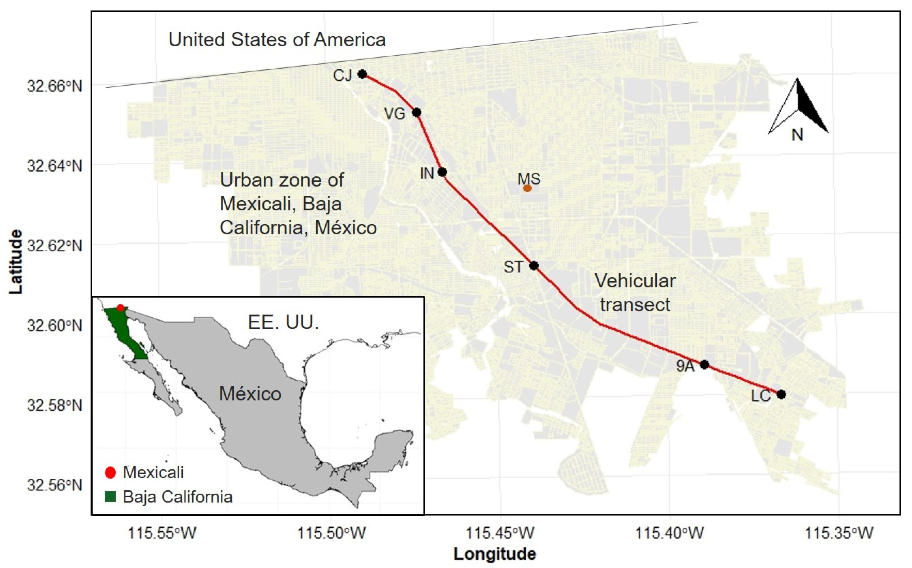
The mobile transects were conducted along Adolfo López Mateos Boulevard, one of the city’s principal arterial roads. The study covered a 15 km transect extending from the international border with the United States toward the southeastern part of the city. This arterial corridor effectively divides the urban area into two distinct sectors (Figure 1).

2.2. Sensor Configuration for Mobile Transects

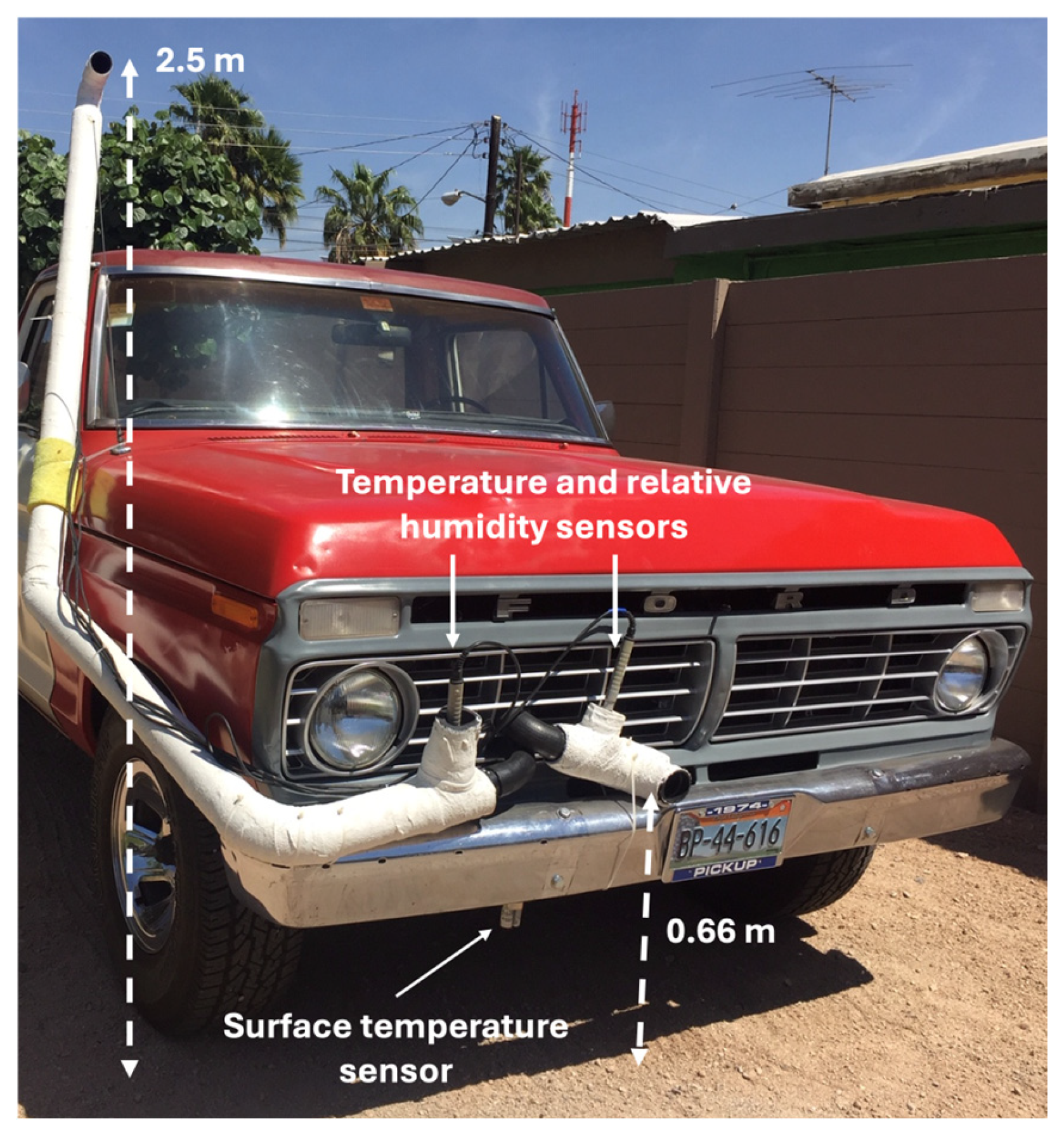
Air temperature measurements were collected along the mobile transect using a vehicle equipped with two air intake inlets. The first inlet was positioned at a height of 0.66 m (T1), corresponding to the original engine air intake height, whereas the second inlet was positioned at 2.5 m (T2), approximately representing the air intake height of public transportation buses. Both inlet heights were measured relative to the pavement surface.

Mobile transects were conducted in both directions along the boulevard at three time periods: 07:00, 14:00, and 19:40 h. Measurements were collected on 9 April 2021, 27 August 2021, and 18 February 2022. These dates were selected as representative days by comparing the meteorological conditions recorded at the reference weather station described in this study with the climatological normals for the 1991–2020 reference period [53].

The vehicle used during the mobile transects was a 1974 pickup truck equipped with a naturally aspirated 302 cubic-inch V8 gasoline engine. It should be emphasized that the engine was not evaluated in terms of its performance, nor was it considered a variable of interest in this study. Instead, the vehicle served exclusively as a mobile platform to ensure continuous air sampling and to transport the measurement instruments along the transect, with vehicle speed varying according to traffic conditions but not exceeding 60 km h⁻¹. Ambient air was sampled solely to measure air temperature and relative humidity, and no engine operating conditions or performance parameters were evaluated.

The air intake inlets were constructed from 2-inch-diameter ABS pipes. The exterior surface was covered with insulation designed for air-conditioning copper pipes, wrapped with a polyester mesh, and coated with white elastomeric paint. Air temperature and relative humidity were measured using Vaisala HMP45C sensors (temperature accuracy: ±0.3 °C at 40 °C and ±0.4 °C at 60 °C; relative humidity accuracy: ±2% RH) [54], while data were recorded using a Campbell Scientific CR23X data logger [55]. The sensors were installed inside the insulated pipes to measure air temperature and relative humidity while minimizing the influence of direct solar radiation and the external environment. This configuration enabled the evaluation of near-surface air temperature variability at two inlet heights representative of engine air intake levels. In addition, surface temperature (Ts) was measured using an SI-111 infrared radiometer (accuracy: ±0.5 °C) [56] connected to the same data logger. The sensor configuration is shown in Figure 2.

2.3. Statistical Analysis of Temperature Variability

Vertical thermal variability during the mobile transects was assessed by analyzing air temperature at the different measurement heights. For this purpose, the standard deviation (SD) and coefficient of variation (CV) were calculated for the morning, afternoon, and nighttime periods of each representative day. These statistical indicators provide quantitative measures of thermal variability relative to the mean and facilitate the identification of conditions associated with greater or lower thermal stability [57].

Analysis of variance (ANOVA) was performed using a significance level of α = 0.05 to determine whether statistically significant differences (p < α) existed among the temperatures recorded at the different measurement heights. In addition, Pearson’s correlation coefficient was calculated for each pair of measurement heights to evaluate the strength of the linear relationship between the corresponding temperature series. This analysis allowed the assessment of whether the temporal evolution of air temperature was consistent across the different measurement heights along each transect [58].

2.4. Correction Factor for Atmospheric Conditions

The correction factor (Cf) was used to quantify the influence of air temperature and atmospheric pressure under standardized engine testing conditions. This theoretical factor is widely applied in engine dynamometer testing to account for the effects of atmospheric conditions on measured engine power and torque by referencing results to standardized sea-level conditions. Atmospheric condition values recorded during the mobile transects were subsequently used as input variables in the model developed by the Society of Automotive Engineers (SAE) [59].

$$\mathrm{C}\mathrm{f}=1.176\left[\left({\displaystyle \frac{990}{P_d}}\right){\left({\displaystyle \frac{T_c+273}{298}}\right)}^{0.5}\right]-0.176$$

(1)

where $P_d$ is the dry air pressure in millibars and $T_c$ is the air temperature in degrees Celsius. The atmospheric pressure variable $P_{atm}$ is represented by the following model:

$$P_{atm}=P_d+P_v$$

(2)

where $P_d$ is the dry air pressure and $P_v$ is the water vapor pressure. The latter can be obtained from measured air temperature and relative humidity (RH) values recorded during the transects using the following expression:

$$P_v={\displaystyle \raisebox{1ex}{$\left(RH\times P_{vs}\right)$}\!\left/ \!\raisebox{-1ex}{$100$}\right.}$$

(3)

The saturation vapor pressure $P_{vs}$ was determined using the Tetens equation [39], which depends on air temperature ($T$).

$$P_{vs}=0.61078exp\left({\displaystyle \frac{17.27T}{237.3+T}}\right)$$

(4)

The calculation of $P_d$ was performed by considering the previously described models and the variables recorded during the transects. The mean atmospheric pressures for the transect days were 1009, 1001, and 1021 millibars, respectively, according to data from the UABC meteorological station (MS). Because atmospheric pressure exhibits relatively low spatial variability at the urban scale considered in this study, a single daily mean value recorded at the meteorological station was used for each sampling campaign.

2.5. Remote Sensing Analysis of Surface Temperature Along the Mobile Transect

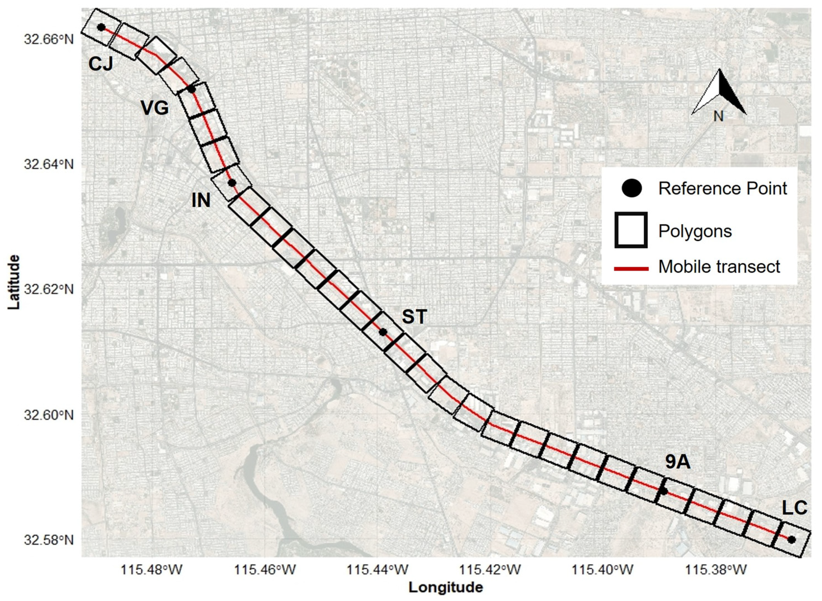
To characterize surface temperature patterns along the vehicle transect, 30 consecutive 500 m × 500 m polygons were delineated over the study area (see Figure 3). Land Surface Temperature (LST) was extracted within each polygon using Landsat 8 Collection 2 Level-2 Science Products (L2SP) with a spatial resolution of 30 m [60]. This procedure was used to compute the mean LST within each polygon and to identify the maximum temperature for each unit. All processing was conducted in R software R 4.5.0, which provides libraries for satellite image processing and data extraction within defined geometries [61,62].

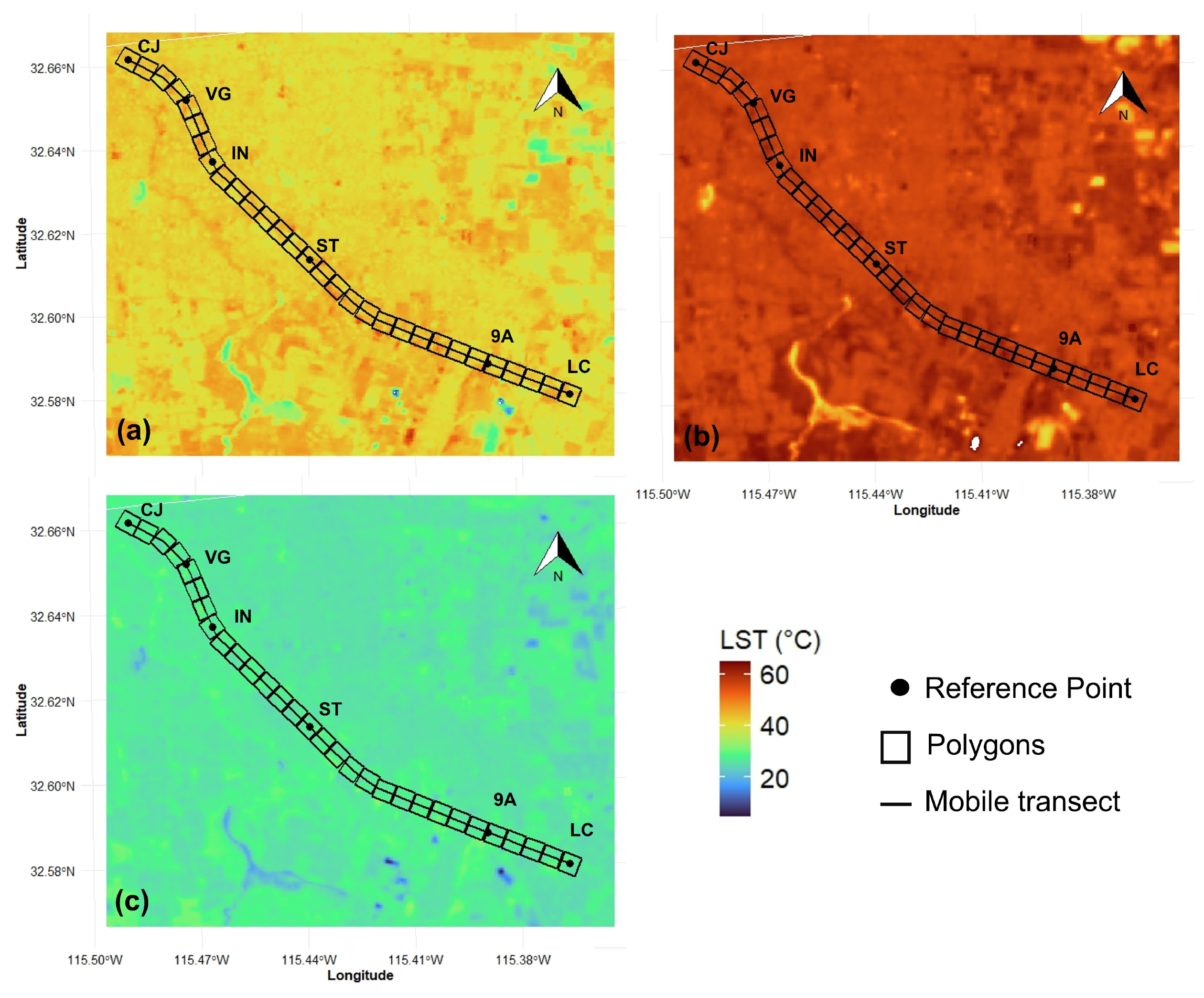
In Landsat L2SP products, Land Surface Temperature (LST) is directly derived by the United States Geological Survey (USGS) from the thermal band B10 of the Thermal Infrared Sensor (TIRS), applying atmospheric correction methods to obtain brightness temperature (BT). In addition, bands B4 and B5 of the Operational Land Imager (OLI) are used to calculate the Normalized Difference Vegetation Index (NDVI), which in turn enables the estimation of surface emissivity based on land-use type [63,64,65]. The Landsat acquisition dates most closely corresponding to the mobile transect surface temperature measurements were 11 April 2021 (10:27 a.m.), 25 August 2021 (11:16 a.m.), and 17 February 2022 (10:16 a.m.). For simplicity, satellite-derived temperatures are hereafter referred to as LST throughout the paper.

3. Results

This section presents the results of near-surface air temperature, the correction factor, land surface temperature, and the analysis of temperature variability.

3.1. Near-Surface Air Temperature Behavior and Theoretical Correction Factor Along Mobile Transectors

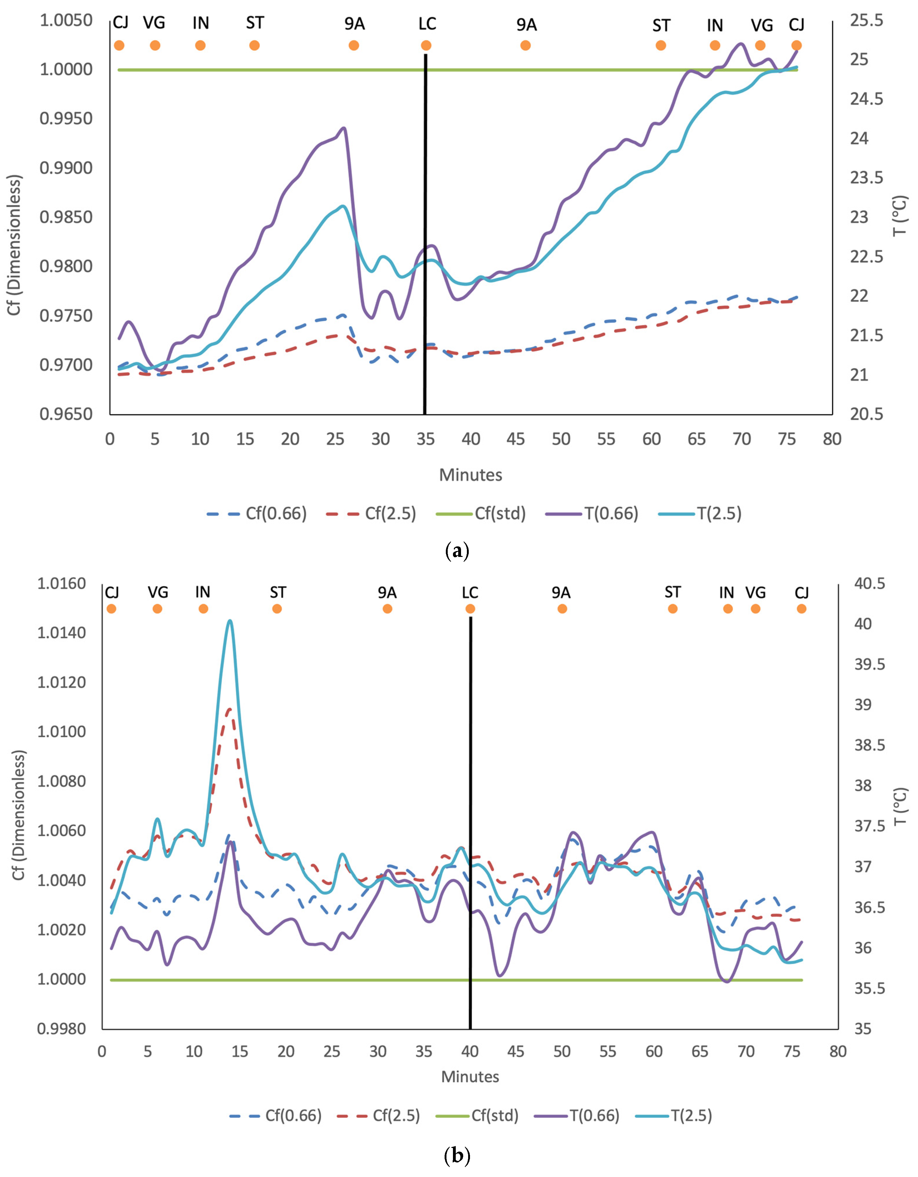
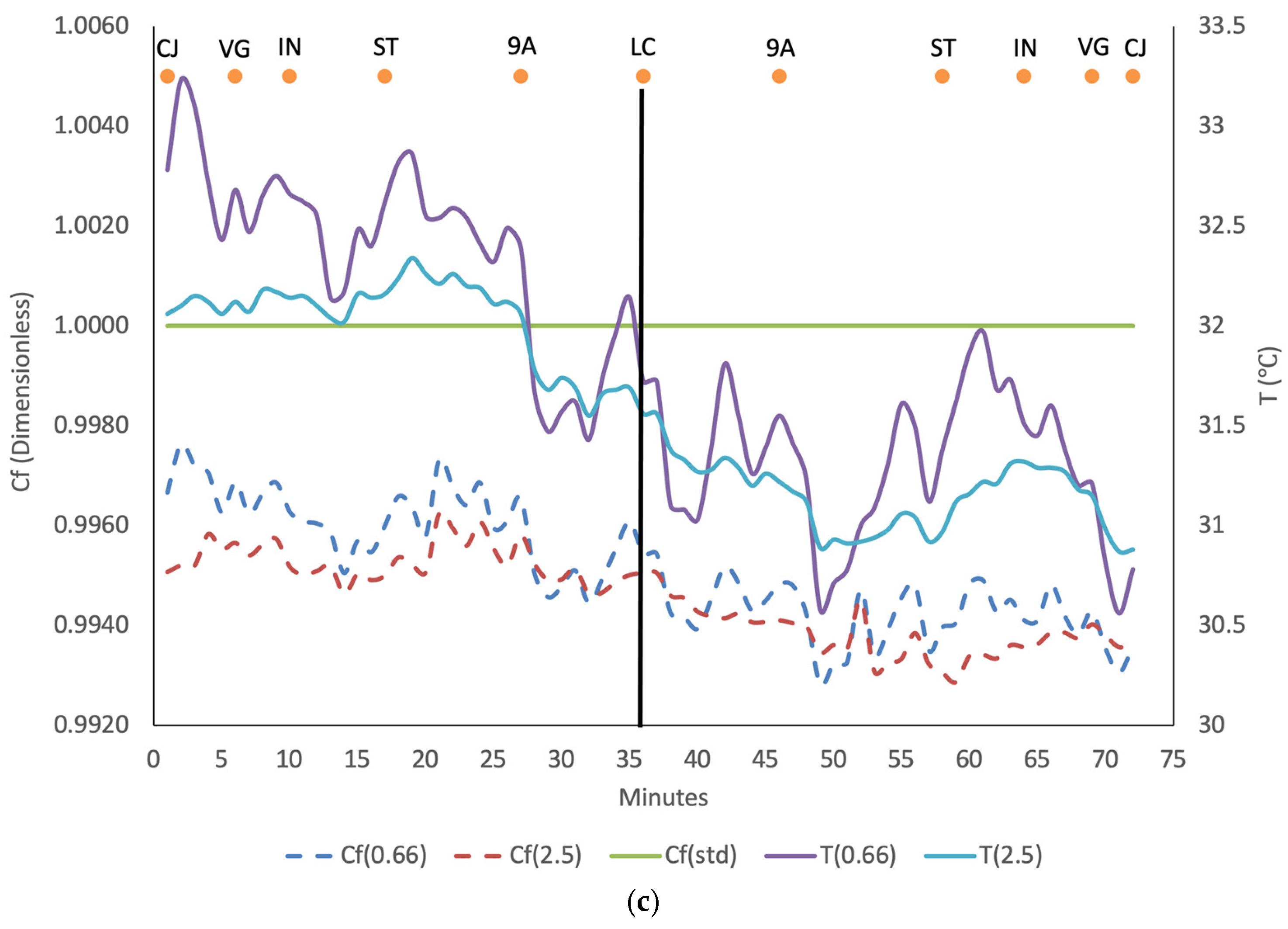
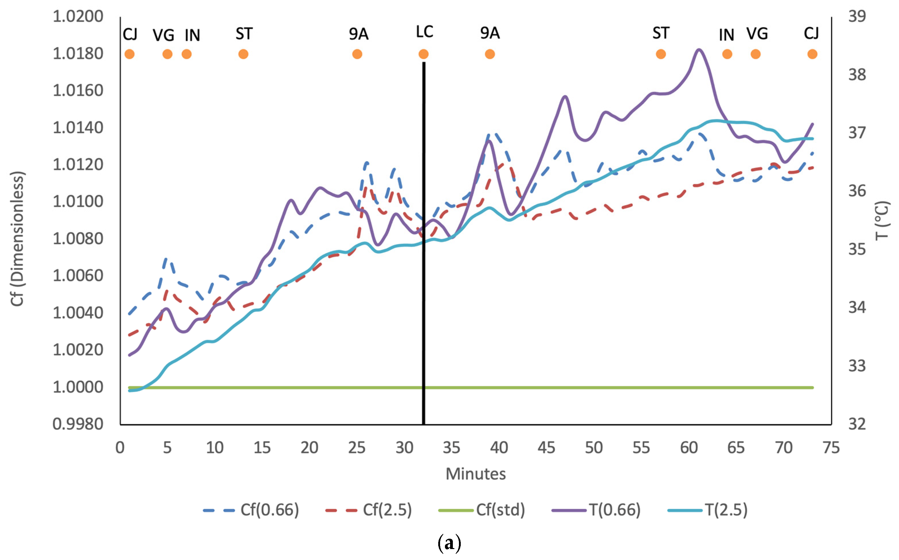
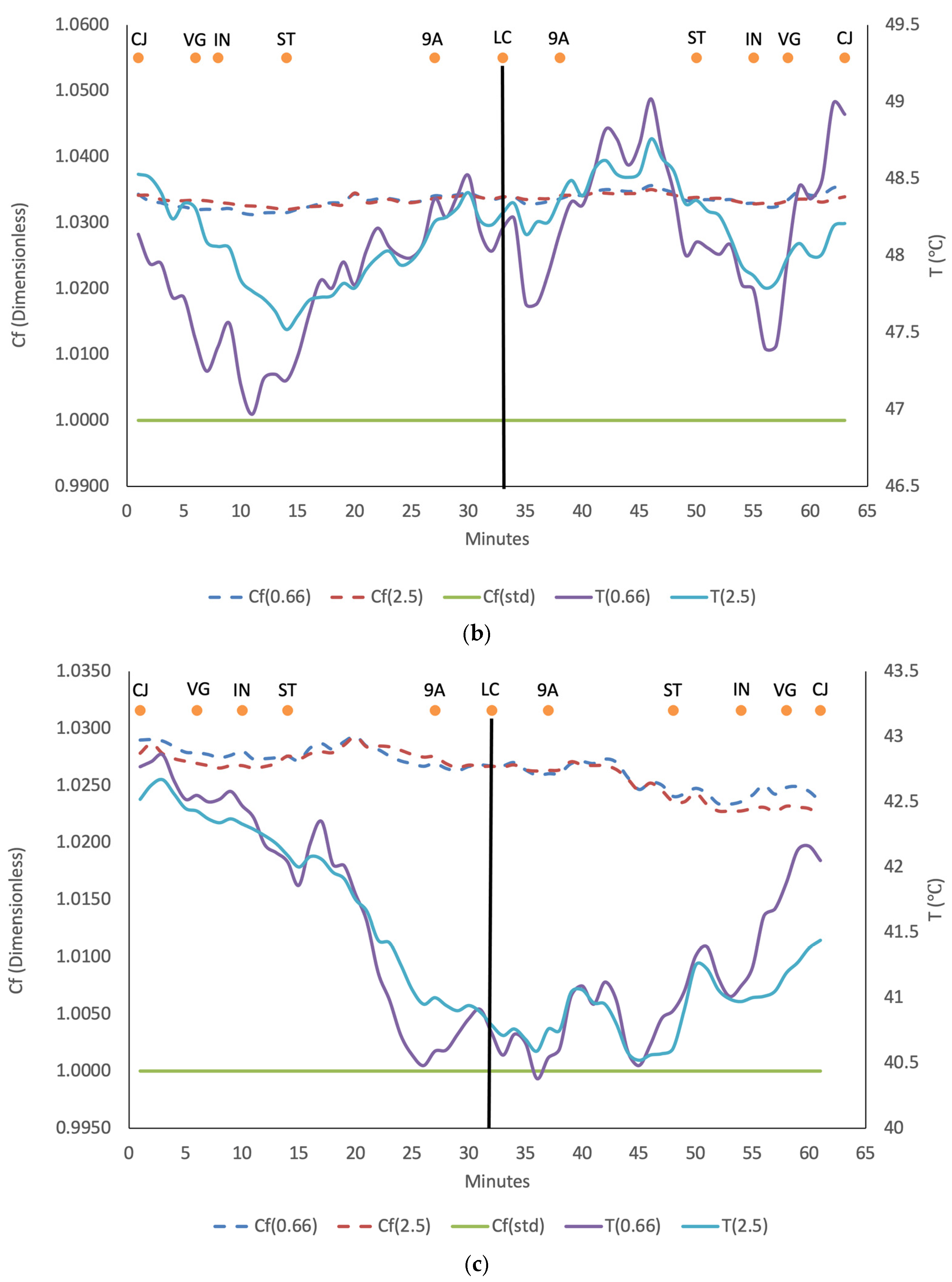
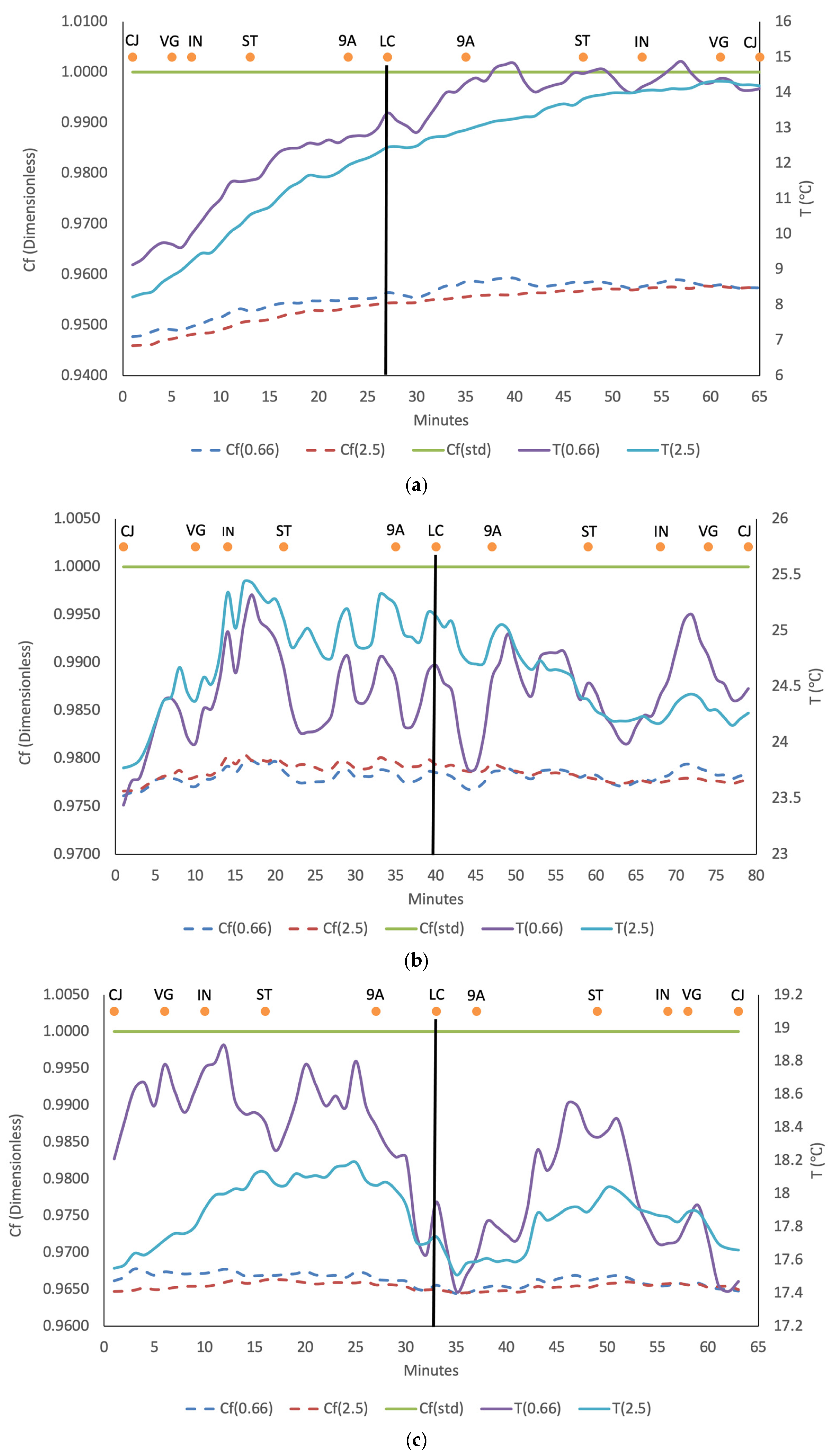
The following three figures illustrate near-surface air temperature and the theoretical correction factor (Cf, green line indicating standard conditions), which serves as a reference. This reference is based on the assumption that air temperature and dry air pressure remain constant at 25 °C and 990 mbar, respectively. These values are typically used as benchmark conditions for internal combustion engine performance specifications at sea level [59]. Transect reference points are indicated by orange dots, while the vertical black line marks the location where the vehicle performed a U-turn to traverse the transect in the opposite direction.

As shown in Figure 4a, Figure 5a and Figure 6a, morning transect temperatures exhibit an increasing trend driven by solar radiation. In contrast, afternoon temperatures (Figure 4b, Figure 5b and Figure 6b) show an approximately constant behavior, while evening temperatures (Figure 4c, Figure 5c and Figure 6c) decrease due to the absence of solar forcing. The behavior of the correction factor (Cf) closely mirrors that of air temperature, reflecting its direct dependence on this primary variable in the mathematical model (see Equation (1)). When measured at two different heights, engine inlet temperatures T(0.66) and T(2.5) are shown in the graphs, respectively.

Upon reaching the southern area of the transect, near the black vertical line in Figure 4, Figure 5 and Figure 6, convergence of air temperatures at both heights is observed, and in some cases, T(2.5) becomes higher than T(0.66). This phenomenon may be attributed to the proximity of the study site to agricultural areas, where intensive land-use patterns characteristic of these environments have been shown to reduce near-surface temperature levels [66,67].

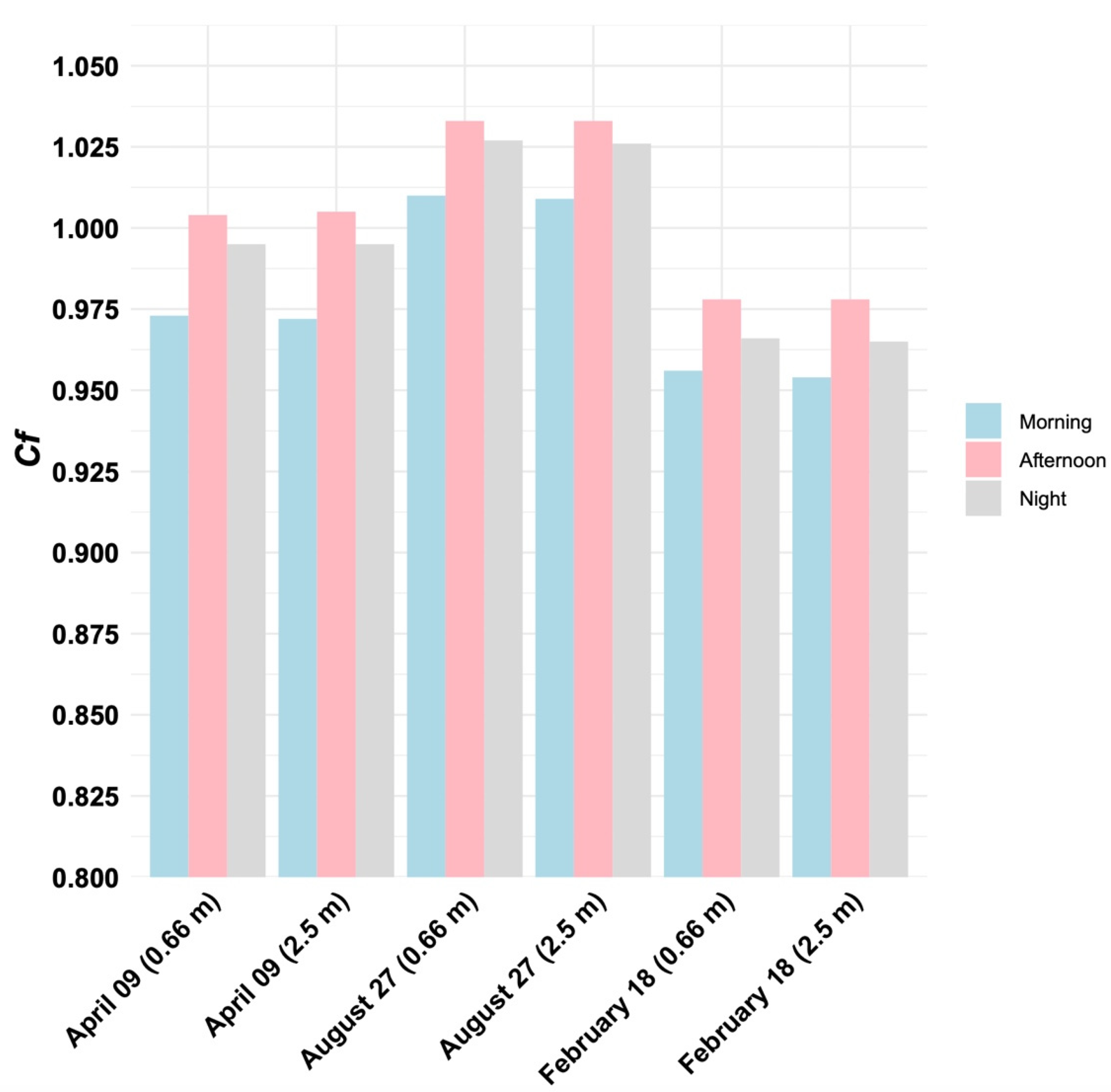
It is noteworthy that temperature measurements at 0.66 m exhibit greater variability compared to those recorded at 2.5 m (see Figure 4, Figure 5 and Figure 6). This is because air temperatures closer to the land–atmosphere interface are more strongly affected by surface heating. Finally, Figure 7 presents the correction factors (Cf) obtained from the mobile transects conducted during the study period.

3.2. Assessment of the Temperature Variability

On 9 April, both morning and nighttime measurements showed higher standard deviation (SD) and coefficient of variation (CV) values at 0.66 m than at 2.5 m, indicating greater air temperature variability near the ground. On 27 August, during all three observation periods, the SD and CV of surface temperature exceeded those recorded at 0.66 m and 2.5 m, indicating greater thermal variability at the surface. A similar pattern was observed on 18 February, when surface temperature exhibited the highest values for both statistical indicators. The analysis of variance (ANOVA) revealed statistically significant differences (p < 0.05) between temperatures measured at 0.66 m and 2.5 m for all three study days and observation periods. Furthermore, on 27 August and 18 February, statistically significant differences were also found between surface temperatures and those measured at 0.66 m. These results indicate distinct thermal behavior across the analyzed measurement levels (

Table 3. Standard deviation (SD) and coefficient of variation (CV) for surface temperature (Ts) and air temperature at 0.66 m and 2.5 m during the mobile transects.

Date of Campaigns	Transect	SD Ts °C	SD T(0.66) °C	SD T(2.5) °C	CV Ts %	CV T(0.66) %	CV T(2.5) %
9 April 2021	Morning	NA	1.231	1.103	NA	5.33	4.85
	Afternoon	1.584	0.454	0.697	2.97	1.25	1.89
	Evening	2.168	0.675	0.486	6.40	2.12	1.54
27 August 2021	Morning	2.273	1.338	1.353	5.80	3.72	3.83
	Afternoon	1.365	0.482	0.292	2.11	1.00	0.61
	Evening	1.818	0.763	0.665	4.03	1.84	1.61
18 February 2022	Morning	2.429	1.647	1.835	16.95	12.60	14.92
	Afternoon	3.581	0.376	0.415	10.23	1.54	1.68
	Evening	1.870	0.421	0.192	9.72	2.31	1.07

NA indicates that the corresponding data were not available.

).

On 9 April, very strong positive correlations were observed between air temperatures measured at 0.66 m and 2.5 m during both the morning (R = 0.949) and nighttime periods (R = 0.918). On 27 August, similarly strong correlations were found between these measurement levels in the morning (R = 0.939) and at night (R = 0.927), whereas the correlation weakened to a moderate level during the afternoon (R = 0.701). In addition, a moderate positive correlation was identified between surface temperature and air temperature at 0.66 m during the morning period (R = 0.694). On 18 February, the strongest correlation between temperatures at 0.66 m and 2.5 m was recorded in the morning (R = 0.973), while moderate correlations were observed during the afternoon (R = 0.534) and evening (R = 0.587). A moderate positive correlation was also found between surface temperature and air temperature at 0.66 m (R = 0.634).

3.3. Remote and Measured Surface Temperature on the Mobile Transect

A summary of the mean and maximum surface temperature values obtained along the vehicular transect is shown in

Table 4. Surface temperatures obtained from the transect and satellite data.

Measurement Description	February	April	August
Maximum transect surface temperature	42.27	58.49	67.29
Maximum land surface temperature	31.52	52.78	64.46
ΔT	10.75	5.71	2.83
Underestimation %	25.43	9.76	4.21
Average transect surface temperature	37.36	53.62	64.75
Average land surface temperature	30.02	48.51	60.9
ΔT	7.34	5.11	3.85
Underestimation %	19.65	9.53	5.95

Transect temperature measurements were conducted on 9 April 2021, 27 August 2021, and 18 February 2022. The satellite images correspond to the following dates: 11 April 2021; 25 August 2021; and 17 February 2022.

, as well as the corresponding land surface temperature (LST) values for the polygons surrounding the transect (Figure 8). A smaller underestimation of LST is observed in April and August, likely due to a more homogeneous spatial distribution of this parameter along the transect. Conversely, during February, the southern segment of the transect showed increased variability in the spatial distribution within the polygons (Figure 8).

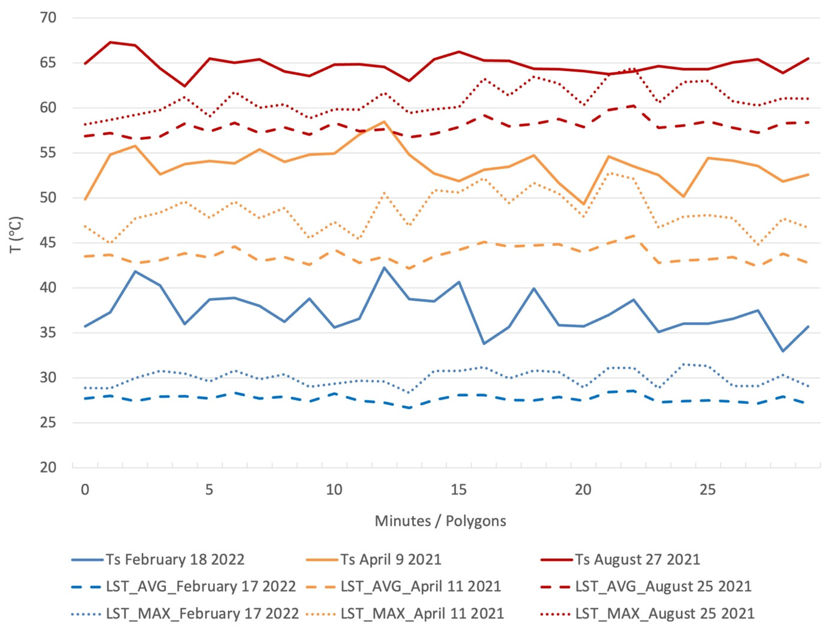
In comparison, the discrepancy between the maximum surface temperatures measured along the transect and those derived from satellite data is more pronounced in February than in April and August. As air temperatures increase toward the warmer months, satellite-derived averages become increasingly consistent with ground-level measurements. In all cases, satellite-derived LST values were lower than in situ measurements by approximately 4–25% for maximum temperatures and 5–19% for mean surface temperatures. This difference may also be attributed to the temporal mismatch between satellite overpass and field measurements, which occurred 3.5, 2.75, and 3.75 h earlier for April, August, and February, respectively. Based on these findings, LST can support the interpretation of transect-based surface temperature patterns with greater confidence during the first two months (February and April). Several studies have shown that, in desert regions, the reliability of Landsat-derived LST improves during the warm months, a period characterized by reduced water vapor [68,69].

Figure 9 presents surface temperature (Ts), juxtaposed with the maximum and average land surface temperature values (LST_MAX and LST_AVG, respectively) corresponding to each polygon encompassing the transect segments in the northwest–southeast direction. In all cases, a strong similarity in the behavior patterns between Ts and LST_AVG can be observed, indicating that heat transfer between the surface and the adjacent air mass is not significantly influenced by external factors. García-Haro [70] previously reported that, during the months analyzed, the highest LST values in the urban area occurred in the southern sector. Accordingly, in this study, both Ts and LST exhibit a congruent spatial pattern. Although occasional convergence between Ts and LST_MAX can be identified, mainly in the southern portion of the study area during the warmer months, satellite-derived temperature values generally remain lower than those recorded along the transect.

4. Discussion

Across all morning transects, the temperature readings obtained at 0.66 m were consistently higher than those recorded at 2.5 m (see Figure 4a, Figure 5a and Figure 6a). This difference is further supported by the mean temperature values presented in

Table 5. Mean air temperature and relative humidity during the mobile transects and corresponding meteorological reference data.

Date of Campaigns	Transect	T(0.66) °C 1	T(2.5) °C 2	RH (0.66) %	RH (2.5) %	UABC Station °C 3	UABC Station 3 RH %	UABC Station MaxT ° C 4	Mexicali Climate Normals ° C 5
9 April 2021	Morning	23.07	22.74	18.91	18.87	22.40	25.61	35	34.1
	Afternoon	36.51	36.54	7.11	6.94	34.21	11.26
	Evening	31.3	31.14	10.13	10.01	31.34	11.08
27 August 2021	Morning	35.97	35.36	15.79	16.04	34	23.68	46	44.3
	Afternoon 1,2	48.02	48.14	8.84	8.65	45.92	13.84
	Evening	41.45	41.39	18.24	17.96	40.92	25.07
18 February 2022	Morning	13.06	12.29	20.25	20.76	11.46	27.42	24	25.9
	Afternoon	24.44	24.66	10.27	10.09	23.68	16.17
	Evening	18.2	17.86	16.54	16.06	18.5	21.92

¹ The maximum air temperature recorded at 0.66 m was 49.19 °C during the transect conducted on 27 August 2021 at 3:11 p.m. ² The maximum air temperature recorded at 2.5 m was 48.83 °C during the transect conducted on 27 August 2021 at 3:13 p.m. ³ The UABC meteorological station is located on the roof of the Institute of Engineering at the Mexicali Campus of the Autonomous University of Baja California. ⁴ Daily maximum air temperature recorded at the UABC meteorological station. ⁵ Long-term climate normal for the daily maximum air temperature in Mexicali. Source: Servicio Meteorológico Nacional, 1991–2020. Standard deviations were 2.3 °C, 2.0 °C, and 2.3 °C for April, August, and February, respectively [53].

. These differences became less pronounced during the afternoon and evening transects because the duration of extreme heat increased as the season transitioned from spring to summer. Consequently, increased surface heating promoted a more homogeneous distribution of air temperature over the relatively flat terrain of the city of Mexicali [71].

With respect to the UABC meteorological station, located approximately 2 km east of the reference point designated as “Independencia” (see Figure 1), air temperature differences reached up to 2.3 °C during the April afternoon transect at both measurement heights, and 2.12 °C and 2.22 °C during the August afternoon transect at 0.66 m and 2.5 m, respectively. As shown in Table 5, the differences between the two measurement heights were less than 1 °C during the February afternoon transects.

Across the three study days, both the standard deviation (SD) and the coefficient of variation (CV) indicated lower temperature variability at 0.66 m and, particularly, at 2.5 m, suggesting greater thermal stability with increasing measurement height. This vertical pattern is consistent with the expected behavior of near-surface urban air temperature, where the influence of surface heating and turbulent mixing generally decreases with height [35].

Higher variability was consistently observed during the morning period at both measurement heights, indicating lower thermal stability than during the afternoon and evening periods. This behavior reflects the stronger influence of rapid surface heating after sunrise and the associated development of thermal gradients within the urban canopy layer.

Moderate correlations between air temperature at 0.66 m and surface temperature (Ts) were identified during the morning transects on 27 August and 18 February, suggesting partial coupling between surface heating and near-surface air temperature under weakly mixed atmospheric conditions. Furthermore, the moderate-to-strong correlations observed between air temperatures measured at 0.66 m and 2.5 m indicate a coherent thermal response at both heights along the mobile transects, as they responded similarly to variations in ambient atmospheric conditions throughout the day.

It is important to note that the correction factor (Cf) is primarily a theoretical parameter designed to account for the influence of atmospheric conditions during engine dynamometer testing and does not represent a direct measurement of engine power output or fuel consumption. Consequently, the findings are interpreted in terms of the potential effects of urban heat and atmospheric conditions on engine performance, as represented by changes in Cf. Values greater than 1.0 indicate that the measured operating conditions require an upward correction to normalize engine performance to standard reference conditions, whereas values below 1.0 require a downward correction. Therefore, the range observed in this study (0.954–1.033) reflects the magnitude of the atmospheric influence on the correction procedure rather than actual gains or losses in engine power. Overall, the Cf theoretically suggests that the engine would produce less power under typical August atmospheric conditions; thus, greater throttle input would be required to compensate for the reduction in power associated with the prevailing atmospheric conditions [4,6].

Unlike carbureted engines, modern electronically controlled internal combustion engines use sensors and engine control units (ECUs) to continuously monitor intake-air temperature, pressure, and oxygen concentration, allowing real-time adjustments of fuel injection and ignition parameters to maintain the desired air–fuel ratio [72,73]. However, these control systems cannot fully compensate for the thermodynamic effects associated with elevated ambient temperatures. Higher intake-air temperatures reduce air density and, consequently, the mass of oxygen available for combustion, which may affect engine performance despite electronic compensation. Furthermore, under extreme thermal conditions, engine control strategies may modify operating parameters to prevent knock and protect engine components [72,73]. Therefore, the elevated temperatures commonly observed in urban heat island environments, such as those occurring in Mexicali during the warm season, may still influence the operating conditions of modern internal combustion engines.

Conversely, the correction factors for the February transects were below 1.0, indicating that the atmospheric conditions during those measurements were more favorable than the standard SAE reference conditions. In contrast, the April transects yielded correction factors close to 1.0, indicating atmospheric conditions that closely approximated the standard reference conditions (see Figure 4).

As shown in Figure 7, the minimum correction factor (Cf) was 0.954, whereas the maximum was 1.033. This difference of 0.079 corresponds to an approximate 8% variation between the winter and extreme warm seasons. Although Cf does not directly represent engine performance or emissions, higher Cf values associated with elevated air temperatures may indicate atmospheric conditions under which greater throttle input would be required to maintain engine performance, potentially contributing to increased exhaust emissions. For example, one study reported a strong positive correlation between air temperature (20–37.5 °C) and emissions of carbon monoxide (CO), sulfur oxides (SOx), nitrogen oxides (NOx), methane, and other pollutants [74]. Similarly, another study found that exhaust emissions from gasoline and diesel vehicles varied across a wide temperature range (−7 to 50 °C) under controlled laboratory conditions, with significant increases in volatile organic compound (VOC) and hydrocarbon emissions observed at high temperatures (>35 °C), which were associated with changes in combustion processes [75].

Beyond their implications for engine performance, these findings also highlight differences between real-world atmospheric conditions and the standardized assumptions used in emission inventory methodologies. The results presented here characterize the atmospheric conditions under which an internal combustion engine may operate in real-world urban environments. These conditions differ from the standardized atmospheric assumptions used by the Intergovernmental Panel on Climate Change (IPCC) to derive emission factors, which are applied in greenhouse gas (GHG) inventory estimations using the Tier 1 methodology [76]. For example, as summarized in

Table 6. Comparison of IPCC reference ambient temperatures and diurnal temperature ranges with those observed in Mexicali.

Seasons	IPCC Ambient Temperature (°C)	IPCC Diurnal Range (°C)	Mexicali Ambient Temperature (°C)	Mexicali Diurnal Range Temperature (°C)
Spring/Fall	16	7 to 24	24.5/27	18 to 31/20 to 33
Winter	2	−7 to 10	16	10 to 22
Summer	29	21 to 38	34.5	28 to 41

, the IPCC assumes the following ambient temperature and diurnal temperature range values.

The summer ambient temperatures assumed by the IPCC correspond to those typically observed in Mexicali during the spring and autumn months, as shown in Table 6. However, summers in Mexicali are characterized by extreme heat, with maximum air temperatures occasionally exceeding 50 °C. The most recent greenhouse gas (GHG) emissions inventory for Baja California, where the study area is located, used the vehicle emission factors proposed by the IPCC [77,78]. These findings suggest that inventories based on these reference conditions may underestimate vehicle emissions in extremely hot climates, although this hypothesis should be evaluated through direct emissions measurements. Furthermore, even when ambient temperatures recorded at a fixed meteorological station are used to calculate the correction factor (Cf), this approach may not fully capture the thermal conditions affecting internal combustion engines because the recorded temperatures are generally lower than those measured during the mobile transects. It is also important to note that atmospheric pressure in Mexicali varies only slightly throughout the year. In contrast, cities located at higher elevations experience substantially lower atmospheric pressure, which can result in considerably greater reductions in the performance of internal combustion engines [79,80].

The present study has several limitations that should be considered when interpreting the results. Recognizing these limitations also identifies opportunities to refine the proposed methodology and guide future research.

First, the analyzed transect covers only a portion of the urban area of Mexicali and, therefore, does not fully capture the spatial variability of the city’s thermal environment. Future studies should incorporate additional transects with different routes and orientations to provide a more comprehensive characterization of the urban thermal environment, as broader spatial sampling has been shown to improve the identification of intra-urban thermal patterns and local climatic variability [57].

In addition, uncertainty in the mobile measurements arises from several factors, including sensor accuracy, the effectiveness of radiation shielding, vehicle movement, airflow disturbances around the instrument, and sensor response time under rapidly changing environmental conditions [33,81]. In this study, the sensors were placed inside insulated tubes that served as passive radiation shields that allowed continuous ambient air circulation. Radiation shielding is widely recognized as essential for minimizing measurement errors associated with direct, reflected, and diffuse solar radiation [82]. Nevertheless, vehicle-induced airflow, localized turbulence, sensor response lag, and rapidly changing urban environmental conditions may still introduce uncertainty into individual measurements [2,5]. Therefore, the reported temperatures should be interpreted as representative of the general spatial thermal patterns observed along the transect rather than as precise point-scale values, which is consistent with previous studies employing mobile monitoring techniques to characterize urban thermal variability [58,83].

Despite these limitations, the methodology provides valuable insights for identifying urban thermal hotspots and generating spatially explicit datasets that may support climate adaptation and urban planning strategies aimed at reducing heat exposure and enhancing urban resilience. Previous studies have highlighted the importance of high-resolution thermal mapping for identifying vulnerable urban areas and supporting evidence-based mitigation and adaptation measures in cities increasingly affected by heat stress [57,84].

Another limitation of this study is that it focuses exclusively on internal combustion engines because the correction factor (Cf) was originally developed to characterize the influence of atmospheric conditions on engine operation under standardized testing conditions, particularly through the effects of air temperature, pressure, and density on engine performance [1]. Consequently, the analysis is limited to propulsion systems whose operation is directly influenced by intake-air properties. However, the increasing adoption of hybrid and battery electric vehicles highlights the need for future research examining how urban heat and climate change may affect alternative propulsion technologies, particularly through their impacts on battery performance, thermal management requirements, energy consumption, and overall vehicle efficiency [85]. Such investigations would contribute to a broader understanding of the interactions between urban climate conditions and the sustainability of future transportation systems.

5. Conclusions

Extreme atmospheric conditions can significantly influence energy-related processes, leading to variations in operating conditions. This study found that the correction factor (Cf), used as a theoretical indicator of the influence of atmospheric conditions on internal combustion engine operation, decreases as air temperatures approach 50 °C and increases under cooler conditions, such as those observed in February. Variations in Cf reached up to 3.35% under the most extreme thermal conditions observed. Under typical conditions in Mexicali, Cf values were generally closer to unity, particularly in February, when values were approximately 4.6% higher than those associated with standardized testing conditions.

Although Cf does not directly represent engine power output, fuel consumption, or emissions, the observed variations suggest that extreme urban heat may influence engine operation indirectly through changes in intake air conditions.

Given the important contribution of mobile sources to criteria pollutant and greenhouse gas (GHG) emission inventories, these findings highlight the need for further research on the influence of extreme atmospheric conditions on vehicle operation and emission processes. The results suggest that incorporating temperature- and pressure-related effects, as represented by correction factors such as Cf, may improve the representation of atmospheric influences in greenhouse gas emission estimation models, particularly in cities exposed to extreme heat.

Future research should extend the proposed methodology to larger urban areas and diverse climatic environments to validate and generalize the findings. Expanding spatial coverage would enable a more comprehensive characterization of urban thermal contrasts and support evidence-based urban planning and climate adaptation strategies. In addition, further studies should assess the effects of extreme atmospheric conditions on the performance, energy efficiency, and operational reliability of emerging clean mobility technologies under real-world urban conditions, thereby contributing to the development of more resilient and sustainable urban transportation systems.

References

1. Sodré, J.R.; Soares, S.M.C. Comparison of engine power correction factors for varying atmospheric conditions. J. Braz. Soc. Mech. Sci. Eng. 2003, 25, 279–284. [Google Scholar] [CrossRef] [Scilit]
2. Birtok-Băneasă, C.; Rațiu, S.; Hepuț, T. Influence of intake air temperature on internal combustion engine operation. IOP Conf. Ser. Mater. Sci. Eng. 2017, 163, 012039. [Google Scholar] [CrossRef] [Scilit]
3. Muhammad, S.K.; Maree, I.E.; Ibraheem, R.R. Influence of intake air temperature on the performance of gasoline engines using a different type of fuel. Al-Qadisiyah J. Eng. Sci. 2022, 15, 229–237. [Google Scholar] [CrossRef] [Scilit]
4. Khaifullizan, M.N.N.; Jaat, N.; Zainal Abidin, S.F.; Darlis, N.; Zahari, I. The Effect of intake air temperature on engine performance and fuel consumption of passenger car. Prog. Eng. Appl. Technol. 2021, 2, 854–865. Available online: https://publisher.uthm.edu.my/periodicals/index.php/peat/article/view/795/1486 (accessed on 15 December 2025).
5. Giechaskiel, B.; Valverde, V.; Kontses, A.; Suarez-Bertoa, R.; Selleri, T.; Melas, A.; Otura, M.; Ferrarese, C.; Martini, G.; Balazs, A.; et al. Effect of extreme temperatures and driving conditions on gaseous pollutants of a Euro 6d-Temp gasoline vehicle. Atmosphere 2021, 12, 1011. [Google Scholar] [CrossRef] [Scilit]
6. Giechaskiel, B.; Komnos, D.; Fontaras, G. Impacts of extreme ambient temperatures and road gradient on energy consumption and CO2 emissions of a Euro 6d-Temp gasoline vehicle. Energies 2021, 14, 6195. [Google Scholar] [CrossRef] [Scilit]
7. Oke, T.R. City size and the urban heat island. Atmos. Environ. (1967) 1973, 7, 769–779. [Google Scholar] [CrossRef] [Scilit]
8. Yun, G.Y.; Ngarambe, J.; Duhirwe, P.N.; Ulpiani, G.; Paolini, R.; Haddad, S.; Vasilakopoulou, K.; Santamouris, M. Predicting the magnitude and the characteristics of the urban heat island in coastal cities in the proximity of desert landforms: The case of Sydney. Sci. Total Environ. 2020, 709, 136068. [Google Scholar] [CrossRef] [Scilit] [PubMed]
9. Busato, F.; Lazzarin, R.M.; Noro, M. Three years of study of the urban heat island in Padua: Experimental results. Sustain. Cities Soc. 2014, 10, 251–258. [Google Scholar] [CrossRef] [Scilit]
10. Oke, T.R. Boundary Layer Climates, 2nd ed.; Routledge: London, UK, 1987. [Google Scholar]
11. Stewart, I.D.; Oke, T.R. Local climate zones for urban temperature studies. Bull. Am. Meteorol. Soc. 2012, 93, 1879–1900. [Google Scholar] [CrossRef] [Scilit]
12. Weng, Q. Thermal infrared remote sensing for urban climate and environmental studies: Methods, applications, and trends. ISPRS J. Photogramm. Remote Sens. 2009, 64, 335–344. [Google Scholar] [CrossRef] [Scilit]
13. Voogt, J.A.; Oke, T.R. Thermal remote sensing of urban climates. Remote Sens. Environ. 2003, 86, 370–384. [Google Scholar] [CrossRef] [Scilit]
14. Li, L.; Tan, Y.; Ying, S.; Yu, Z.; Li, Z.; Lan, H. Impact of land cover and population density on land surface temperature: Case study in Wuhan, China. J. Appl. Remote Sens. 2013, 7, 073573. [Google Scholar] [CrossRef] [Scilit]
15. Tomlinson, C.J.; Chapman, L.; Thornes, J.E.; Baker, C.J. Including the urban heat island in spatial heat health risk assessment strategies: A case study for Birmingham, UK. Int. J. Health Geogr. 2011, 10, 42. [Google Scholar] [CrossRef] [Scilit] [PubMed]
16. Bruse, M.; Fleer, H. Simulating surface–plant–air interactions inside urban environments with a three-dimensional numerical model. Environ. Model. Softw. 1998, 13, 373–384. [Google Scholar] [CrossRef] [Scilit]
17. Salamanca, F.; Martilli, A.; Tewari, M.; Chen, F. A study of the urban boundary layer using different urban parameterizations and high-resolution urban canopy parameters with the WRF model. J. Appl. Meteorol. Climatol. 2011, 50, 1107–1128. [Google Scholar] [CrossRef] [Scilit]
18. Meier, F.; Fenner, D.; Grassmann, T.; Otto, M.; Scherer, D. Crowdsourcing air temperature from citizen weather stations for urban climate research. Urban Clim. 2017, 19, 170–191. [Google Scholar] [CrossRef] [Scilit]
19. Muller, C.L.; Chapman, L.; Johnston, S.; Kidd, C.; Illingworth, S.; Foody, G.; Overeem, A.; Leigh, R.R. Crowdsourcing for climate and atmospheric sciences: Current status and future potential. Int. J. Climatol. 2015, 35, 3185–3203. [Google Scholar] [CrossRef] [Scilit]
20. Bechtel, B.; Alexander, P.J.; Böhner, J.; Ching, J.; Conrad, O.; Feddema, J.; Mills, G.; See, L.; Stewart, I.D. Mapping Local Climate Zones for a worldwide database of the form and function of cities. ISPRS Int. J. Geo-Inf. 2015, 4, 199–219. [Google Scholar] [CrossRef] [Scilit]
21. Grimmond, C.S.B.; Oke, T.R. Heat storage in urban areas: Local-scale observations and evaluation of a simple model. J. Appl. Meteorol. 1999, 38, 922–940. [Google Scholar] [CrossRef] [Scilit] [PubMed]
22. Offerle, B.; Grimmond, C.S.B.; Oke, T.R. Parameterization of net all-wave radiation for urban areas. J. Appl. Meteorol. Climatol. 2003, 42, 1157–1173. [Google Scholar] [CrossRef] [Scilit] [PubMed]
23. Matzarakis, A.; Mayer, H.; Iziomon, M.G. Applications of a universal thermal index: Physiological equivalent temperature. Int. J. Biometeorol. 1999, 43, 76–84. [Google Scholar] [CrossRef] [Scilit] [PubMed]
24. Jendritzky, G.; de Dear, R.; Havenith, G. UTCI—Why another thermal index? Int. J. Biometeorol. 2012, 56, 421–428. [Google Scholar] [CrossRef] [Scilit] [PubMed]
25. Pigliautile, I.; Pisello, A.L. A new wearable monitoring system for investigating pedestrians’ environmental conditions: Development of the experimental tool and start-up findings. Sci. Total Environ. 2018, 630, 690–706. [Google Scholar] [CrossRef] [Scilit] [PubMed]
26. Pigliautile, I.; Pisello, A.L. Environmental data clustering analysis through wearable sensing techniques: New bottom-up process aimed to identify intra-urban granular morphologies from pedestrian transects. Build. Environ. 2020, 171, 106641. [Google Scholar] [CrossRef] [Scilit]
27. Romero Rodríguez, L.; Sánchez Ramos, J.; Sánchez de la Flor, F.J.; Álvarez Domínguez, S. Analyzing the urban heat island: Comprehensive methodology for data gathering and optimal design of mobile transects. Sustain. Cities Soc. 2020, 55, 102027. [Google Scholar] [CrossRef] [Scilit]
28. Romero Rodríguez, L.; Sánchez Ramos, J.; Molina Félix, J.L.; Álvarez Domínguez, S. Urban-scale air temperature estimation: Development of an empirical model based on mobile transects. Sustain. Cities Soc. 2020, 63, 102471. [Google Scholar] [CrossRef] [Scilit]
29. Kousis, I.; Pigliautile, I.; Pisello, A.L. Investigating the intra-urban thermal and air quality environment: New transect sensing methodology and measurements. Measurement 2023, 219, 113210. [Google Scholar] [CrossRef] [Scilit]
30. Sun, C.-Y.; Brazel, A.J.; Chow, W.T.L.; Hedquist, B.C.; Prashad, L. Desert heat island study in winter by mobile transect and remote sensing techniques. Theor. Appl. Climatol. 2009, 98, 323–335. [Google Scholar] [CrossRef] [Scilit]
31. Sun, C.-Y. A street thermal environment study in summer by the mobile transect technique. Theor. Appl. Climatol. 2011, 106, 433–442. [Google Scholar] [CrossRef] [Scilit]
32. Jaiswal, N.; Deb, S.K.; Panda, S.K.; Mandal, A.K.; Khan, A.W.; Kishtawal, C.M. Estimation of intra-urban thermal variability in Ahmedabad city using moving vehicle transects. J. Earth Syst. Sci. 2023, 132, 41. [Google Scholar] [CrossRef] [Scilit]
33. Tsin, P.K.; Knudby, A.; Krayenhoff, E.S.; Ho, H.C.; Brauer, M.; Henderson, S.B. Microscale mobile monitoring of urban air temperature. Urban Clim. 2016, 18, 58–72. [Google Scholar] [CrossRef] [Scilit]
34. Hart, M.A.; Sailor, D.J. Quantifying the influence of land-use and surface characteristics on spatial variability in the urban heat island. Theor. Appl. Climatol. 2009, 95, 397–406. [Google Scholar] [CrossRef] [Scilit]
35. Oke, T.R.; Mills, G.; Christen, A.; Voogt, J.A. Urban Climates; Cambridge University Press: Cambridge, UK, 2017. [Google Scholar] [CrossRef] [Scilit]
36. Middel, A.; Häb, K.; Brazel, A.J.; Martin, C.; Guhathakurta, S. Impact of urban form and design on mid-afternoon microclimate in Phoenix Local Climate Zones. Landsc. Urban Plan. 2014, 122, 16–28. [Google Scholar] [CrossRef] [Scilit]
37. Brandsma, T.; Wolters, D. Measurement and statistical modeling of the urban heat island of the city of Utrecht (the Netherlands). J. Appl. Meteorol. Climatol. 2012, 51, 1046–1060. [Google Scholar] [CrossRef] [Scilit]
38. Weng, Q.; Fu, P.; Gao, F. Satellite Remote Sensing of Surface Urban Heat Islands: Progress, Challenges, and Perspectives. Remote Sens. 2019, 11, 48. [Google Scholar] [CrossRef] [Scilit]
39. Leconte, F.; Bouyer, J.; Claverie, R.; Pétrissans, M. Using Local Climate Zone scheme for UHI assessment: Evaluation of the method using mobile measurements. Build. Environ. 2015, 83, 39–49. [Google Scholar] [CrossRef] [Scilit]
40. Coutts, A.M.; Harris, R.J.; Phan, T.; Livesley, S.J.; Williams, N.S.G.; Tapper, N.J. Thermal infrared remote sensing of urban heat: Hotspots, vegetation, and an assessment of techniques for use in urban planning. Remote Sens. Environ. 2016, 186, 637–651. [Google Scholar] [CrossRef] [Scilit]
41. Jain, M.; Dimri, A.P.; Niyogi, D. Land-air interactions over urban-rural transects using satellite observations: Analysis over Delhi, India from 1991–2016. Remote Sens. 2017, 9, 1283. [Google Scholar] [CrossRef] [Scilit]
42. Sithole, K.; Odindi, J.O. Determination of urban thermal characteristics on an urban/rural land cover gradient using remotely sensed data. S. Afr. J. Geomat. 2015, 4, 384–396. [Google Scholar] [CrossRef] [Scilit]
43. Mugo, R.; Waswa, R.; Nyaga, J.W.; Ndubi, A.; Adams, E.C.; Flores-Anderson, A.I. Quantifying land use land cover changes in the Lake Victoria Basin using satellite remote sensing: The trends and drivers between 1985 and 2014. Remote Sens. 2020, 12, 2829. [Google Scholar] [CrossRef] [Scilit]
44. Talukdar, S.; Singha, P.; Mahato, S.; Shahfahad, P.; Pal, S.; Liou, Y.A.; Rahman, A. Land-use land-cover classification by machine learning classifiers for satellite observations—A review. Remote Sens. 2020, 12, 1135. [Google Scholar] [CrossRef] [Scilit]
45. Li, Z.-L.; Wu, H.; Duan, S.-B.; Zhao, W.; Ren, H.; Liu, X.; Leng, P.; Tang, R.; Ye, X.; Zhu, J.; et al. Satellite remote sensing of global land surface temperature: Definition, methods, products, and applications. Rev. Geophys. 2023, 61, e2022RG000777. [Google Scholar] [CrossRef] [Scilit]
46. Kavouras, I.G.; DuBois, D.W.; Nikolich, G.; Corral Avittia, A.Y.; Etyemezian, V. Particulate dust emission factors from unpaved roads in the U.S.–Mexico border semi-arid region. J. Arid Environ. 2016, 124, 189–192. [Google Scholar] [CrossRef] [Scilit]
47. Hassan, H.; Saraga, D.; Kumar, P.; Kakosimos, K.E. Vehicle-induced fugitive particulate matter emissions in a city of arid desert climate. Atmos. Environ. 2020, 229, 117450. [Google Scholar] [CrossRef] [Scilit]
48. Flores Jiménez, D.E.; de los Ángeles Santos Gómez, M.; Santillán Soto, N. Emisiones vehiculares de dióxido de carbono al cruzar una zona fronteriza al noroeste de México antes y durante la incidencia del COVID-19. CIENCIA Ergo-Sum 2024, 31. [Google Scholar] [CrossRef] [Scilit]
49. García-Cueto, O.R.; Santillán-Soto, N.; Quintero-Núñez, M.; Ojeda-Benítez, S.; Velázquez-Limón, N. Extreme temperature scenarios in Mexicali, Mexico under climate change conditions. Atmosphere 2013, 4, 509–520. [Google Scholar] [CrossRef] [Scilit]
50. García-Cueto, O.R.; Santillán-Soto, N. Modeling Extreme Climate Events: Two Case Studies in México; Intechopen: London, UK, 2012; Available online: https://www.intechopen.com/books/climate-models/modeling-extreme-climate-events-two-case-studies-in-mexico (accessed on 4 August 2025).
51. CONAGUA. Comisión Nacional del Agua. Informe del Comité Técnico de Operación de Obras Hidráulicas. Available online: https://www.gob.mx/conagua/prensa/informe-del-comite-tecnico-de-operacion-de-obras-hidraulicas-371179?idiom=es (accessed on 24 June 2026).
52. García-Cueto, R.; Ley-García, J. Las ondas cálidas en Mexicali, Baja California, México: Morbilidad, mortalidad y vulnerabilidad al calor. Investig. Geográficas 2024, 114, e60848. [Google Scholar] [CrossRef] [Scilit]
53. Servicio Meteorológico Nacional. Normales Climatológicas de Baja California 1991–2020. Available online: https://smn.conagua.gob.mx/es/climatologia/informacion-climatologica/normales-climatologicas-por-estado?estado=bc (accessed on 16 June 2026).
54. Campbell Scientific. HMP45C-L Temperature and Relative Humidity Probe. 2025. Available online: https://www.campbellsci.in/hmp45c-l (accessed on 2 June 2025).
55. Campbell Scientific. CR23X Micrologger for Data Acquisition. 2025. Available online: https://www.campbellsci.in/cr23x (accessed on 2 June 2025).
56. Campbell Scientific. SI-111 Infrared Radiometer with Standard Field of View. 2025. Available online: https://www.campbellsci.in/si-111 (accessed on 10 December 2025).
57. Kousis, I.; Pigliautile, I.; Pisello, A.L. Intra-Urban Microclimate Investigation in Urban Heat Island through a Novel Mobile Monitoring System. Sci. Rep. 2021, 11, 9732. [Google Scholar] [CrossRef] [Scilit] [PubMed]
58. Martinez-Soto, A.; Vera-Fonseca, M.; Valenzuela-Toledo, P.; Melillan-Raguileo, A.; Shupler, M. Heat on the Move: Contrasting Mobile and Fixed Insights into Temuco’s Urban Heat Islands. Sensors 2025, 25, 1251. [Google Scholar] [CrossRef] [Scilit] [PubMed]
59. SAE J1349; Engine Power Test Code—Spark Ignition and Compression Ignition Net Power Rating. SAE International: Warrendale, PA, USA, 2004.
60. U.S. Geological Survey. EarthExplorer. 2025. Available online: https://earthexplorer.usgs.gov/ (accessed on 26 August 2025).
61. Ghosh, A.; Hijmans, R.J. Remote Sensing Image Analysis with R. University of California. 2023. Available online: https://rspatial.org/rs/rs.pdf (accessed on 27 August 2025).
62. USGS. Landsat 8–9 Collection 2 Level-2 Science Product Guide (Versión 2.0, LSDS-1619). Department of the Interior U.S. Geological Survey. 2020. Available online: https://d9-wret.s3.us-west-2.amazonaws.com/assets/palladium/production/s3fs-public/atoms/files/LSDS-1619_Landsat8-C2-L2-ScienceProductGuide-v2.pdf (accessed on 27 August 2025).
63. USGS. Landsat 8 Collection 1 (C1) Land Surface Reflectance Code (LaSRC) Product Guide (Versión 3.0). Department of the Interior U.S. Geological Survey . 2020. Internal document LSDS-1368. Available online: https://d9-wret.s3.us-west-2.amazonaws.com/assets/palladium/production/s3fs-public/atoms/files/LSDS-1368_L8_C1-LandSurfaceReflectanceCode-LASRC_ProductGuide-v3.pdf (accessed on 27 August 2025).
64. USGS. Landsat 8-9 Collection 2 (C2) Level 2 Science Product (L2SP) Guide (Versión 6.0). Department of the Interior U.S. Geological Survey. 2024. Internal document LSDS-1619. Available online: https://d9-wret.s3.us-west-2.amazonaws.com/assets/palladium/production/s3fs-public/media/files/LSDS-1619_Landsat8-9-Collection2-Level2-Science-Product-Guide-v6.pdf (accessed on 27 August 2025).
65. Sobrino, J.A.; Jiménez-Muñoz, J.C.; Paolini, L. Land surface temperature retrieval from LANDSAT TM 5. Remote Sens. Environ. 2004, 90, 434–440. [Google Scholar] [CrossRef] [Scilit]
66. García-Cueto, O.R.; Tejeda Martínez, A.; Bojórquez Morales, G. Urbanization effects upon the air temperature in Mexicali, B.C. México. Atmósfera 2009, 22, 349–365. Available online: https://www.revistascca.unam.mx/atm/index.php/atm/article/view/8634 (accessed on 25 September 2025).
67. Villanueva-Solís, J. Urban Heat Island Mitigation and Urban Planning: The Case of the Mexicali, B.C. Mexico. Am. J. Clim. Chang. 2017, 6, 22–39. [Google Scholar] [CrossRef]
68. Pan, X.; Zhang, F.; Gong, W.; Sun, J. Applicability of downscaling land surface temperature by Random Forest in a desert region. Sci. Rep. 2018, 8, 10555. [Google Scholar] [CrossRef] [Scilit] [PubMed]
69. Arabi Aliabad, F.; Zare, M.; Ghafarian Malamiri, H.; Ghaderpour, E. Improving the accuracy of Landsat 8 land surface temperature in arid regions by MODIS water vapor imagery. Atmosphere 2023, 14, 1589. [Google Scholar] [CrossRef] [Scilit]
70. García Haro, A.; Arellano, B.; Roca, J. Integrating multi source remote sensing and spatial metrics to quantify urban park design effects on surface cool islands in Mexicali, Mexico. Remote Sens. 2025, 17, 3296. [Google Scholar] [CrossRef] [Scilit]
71. García-Cueto, R. Análisis de Balances Energéticos Atmosféricos en Puebla, Mexicali y Ciudad de México. 2016. Available online: http://140.84.163.2:8080/xmlui/handle/publicaciones/265 (accessed on 25 September 2025).
72. Internal Combustion Engine Fundamentals; Heywood, J.B. Internal Combustion Engine Fundamentals, 2nd ed.; McGraw-Hill Education: New York, NY, USA, 2018. [Google Scholar]
73. Robert Bosch GmbH. Bosch Automotive Handbook, 10th ed.; Wiley: Hoboken, NJ, USA, 2018. [Google Scholar]
74. Hoseinifar, S.E.; Shafiepour Motlagh, M.; Ashrafi, K.; Ahadi, M.R. The Effects of Seasonal Changes of Ambient Temperature and Humidity on Exhaust Pipe Emissions and Greenhouse Gases. Pollution 2023, 9, 1808–1818. [Google Scholar] [CrossRef]
75. Ferrarese, C.; Franzetti, J.; Selleri, T.; Suarez-Bertoa, R. VOC Emissions from Euro 6 Vehicles. Environ. Sci. Eur. 2024, 36, 27. [Google Scholar] [CrossRef] [Scilit]
76. IPCC. Revised 1996 IPCC Guidelines for National Greenhouse Gas Inventories: Reference Manual; IPCC: Geneva, Switzerland, 1996; Volume 3, pp. 61–80. Available online: https://www.ipcc-nggip.iges.or.jp/public/gl/invs6a.html (accessed on 16 October 2025).
77. Gobierno de Baja California. Emisiones de Gases de Efecto Invernadero en Baja California y Proyecciones de Casos de Referencia 1990–2025. 2010. Available online: https://www.bajacalifornia.gob.mx/Documentos/sest/desarrollo_sustentable/Programas_Proyectos/Cambio_Climatico/Inventarios_Emision_Gases_Efecto_Invernadero/EMISIONES-DE-GASES-DE-EFECTO-INVERNADERO-EN-BC_PROYECCIONES_CASOS%20REFERENCIA_1990-2025.pdf (accessed on 16 October 2025).
78. Centro Mario Molina para Estudios Estratégicos sobre Energía y Medio Ambiente; Secretaría de Protección al Ambiente del Estado de Baja California. Inventario de Emisiones de Gases de Efecto Invernadero del Estado de Baja California (Año Base 2005). 2007. Available online: https://www.bajacalifornia.gob.mx/Documentos/sest/desarrollo_sustentable/Programas_Proyectos/Cambio_Climatico/Inventarios_Emision_Gases_Efecto_Invernadero/INVENTARIO-EMISIONES-GASES-EFECTO-INVERNADERO-DEL-ESTADO-DE-BC_2007.pdf (accessed on 16 October 2025).
79. Ceballos, J.J.; Melgar, A.; Tinaut, F.V. Influence of environmental changes due to altitude on performance, fuel consumption and emissions of a naturally aspirated diesel engine. Energies 2021, 14, 5346. [Google Scholar] [CrossRef] [Scilit]
80. González, L.; Vaca, C.; Álvarez, H. Effects of altitude in the performance of a spark ignition internal combustion engine. Mater. Today Proc. 2022, 49, 72–78. [Google Scholar] [CrossRef] [Scilit]
81. Häb, K.; Ruddell, B.L.; Middel, A. Sensor lag correction for mobile urban microclimate measurements. Urban Clim. 2015, 14, 622–635. [Google Scholar] [CrossRef] [Scilit]
82. Lipina, P.; Procházka, J.; Brabec, M.; Novotný, D.; Geletič, J.; Lehnert, M. Effect of radiation shield type on air temperature measured by urban station: Extensive intercomparison study in Ostrava, Czech Republic. J. Appl. Meteorol. Climatol. 2026, 65, 587–605. [Google Scholar] [CrossRef] [Scilit]
83. Kousis, I.; Pigliautile, I.; Pisello, A.L. A Mobile Vehicle-Based Methodology for Dynamic Microclimate Analysis. Int. J. Environ. Res. 2021, 15, 893–901. [Google Scholar] [CrossRef] [Scilit] [PubMed]
84. Revi, A.; Satterthwaite, D.; Aragón-Durand, F.; Corfee-Morlot, J.; Kiunsi, R.; Pelling, M.; Roberts, D.; Solecki, W. Urban Areas. In Climate Change 2022: Impacts Adaptation and Vulnerability; Pörtner, H.-O., Roberts, D.C., Tignor, M., Poloczanska, E.S., Mintenbeck, K., Alegría, A., Craig, M., Langsdorf, S., Löschke, S., Möller, V., et al., Eds.; Cambridge University Press: Cambridge, UK, 2022; pp. 907–1040. [Google Scholar] [CrossRef] [Scilit]
85. Hwang, F.S.; Confrey, T.; Reidy, C.; Picovici, D.; Callaghan, D.; Culliton, D.; Nolan, C. Review of battery thermal management systems in electric vehicles. Renew. Sustain. Energy Rev. 2024, 192, 114171. [Google Scholar] [CrossRef] [Scilit]
Figure 1. Study area. The urban surface of Mexicali, Baja California. The mobile transect is delineated by a red line, and the reference points are annotated with their respective identifications: CJ Calle Juárez, VG Vicente Guerrero, IN Independencia, ST Sánchez Taboada, 9A Calle Novena, LC Lázaro Cárdenas, and MS refers to the UABC meteorological station.
Urbansci 10 00477 g001
Figure 2. Vehicle used for the mobile transects, showing the two air intake inlets installed at different heights for air temperature and relative humidity measurements.
Urbansci 10 00477 g002
Figure 3. Consecutive 500 m × 500 m polygons, delineated by black outlines, are shown along the mobile transect indicated by the red line.
Urbansci 10 00477 g003
Figure 4. Temperature and correction factors on 9 April 2021. The experimental campaigns are designated by the following transects: morning (a), afternoon (b), and night (c).
Urbansci 10 00477 g004aUrbansci 10 00477 g004b
Figure 5. Temperature and correction factors on 27 August 2021. The experimental campaigns are designated by the following transects: morning (a), afternoon (b), and night (c).
Urbansci 10 00477 g005aUrbansci 10 00477 g005b
Figure 6. Temperature and correction factors on 18 February 2022. The experimental campaigns are designated by the following transects: morning (a), afternoon (b), and night (c).
Urbansci 10 00477 g006
Figure 7. Correction Factor (Cf) calculated based on the atmospheric conditions recorded during the transect.
Urbansci 10 00477 g007
Figure 8. Land Surface Temperature (LST) in the study area measured on the following dates and times: (a) 11 April 2021, at 10:27 a.m.; (b) 25 August 2021, at 11:16 a.m.; and (c) 17 February 2022, at 10:16 a.m., all in Pacific Daylight Time (PDT).
Urbansci 10 00477 g008
Figure 9. Surface temperatures from the transect and satellite images. The x-axis denotes the temporal progression in minutes, encompassing the initial 30 min of the northwest–southeast transect, together with the average temperature of the 30 polygons derived from satellite imagery.
Urbansci 10 00477 g009