Connecting Parks and People: Recreational Flow and Barrier Modeling in the City of Leipzig, Germany

Abstract

In an increasingly urbanized world, ensuring equitable access to urban green spaces (UGS) is essential for human well-being. Previous studies have largely focused on measuring proximity or availability of UGS, often neglecting the role of the walkable environment and the interaction between supply, demand, and movement flows. To address this gap, we develop a novel modeling framework that integrates the Detour Index (DI) and Local Significance (LS) to jointly capture physical barriers and recreational flows within urban street networks. Using openly available data from OpenStreetMap and Urban Atlas, we model the walkable environment in Leipzig, Germany, at a high spatial resolution. The approach enables the identification of inefficient routes, potential barriers, and areas of high use intensity, providing actionable insights for urban planning. By combining network-based accessibility with flow-based indicators, our method advances existing approaches that rely on static distance measures. The analyses of different planning alternatives further demonstrate how changes in urban structure affect accessibility and crowding patterns. The framework is transferable and based on open data, providing a foundation for future research to integrate behavioral factors and richer datasets to further refine accessibility modeling.

1. Introduction

In the Anthropocene, rapid urbanization takes place globally. A total of 55% of the global population were living in cities by 2018 and 68% are projected to do so in 2050. A growing urban population depends increasingly on urban ecosystems [1,2]. Ecosystems supply ecosystem services (ES) which are critical to human well-being [3]. Living in proximity of urban green spaces (UGS) can help alleviate the impacts of climate change on an aging urban population, as well as improve overall public health in cities [4]. Thus, having access to UGS can enhance urban inhabitants’ quality of life [5]. Likewise, the United Nations have agreed to provide universal access to public green spaces by 2030 in Sustainable Development Goal 11.7 [6].

In Europe, 74% of the population are living in cities [2]. Here, the population pressure on UGS might be amplified by the compact city paradigm, which is popular among European city planners; a more compact city can result in shorter traveling distances but also in more overcrowding effects [7]. Accordingly, more people living in proximity to and benefiting from an UGS also increases the pressure on its ecological functions. In order to detect such mismatches in green space supply and demand and to provide equal access to UGS, mapping UGS accessibility is key [8].

The walkable environment—the space in between urban dwellers and UGS—not only affects the quality of ES and, thus, the accessibility of UGS [9], but availability of UGS in a walking distance can also improve overall public health and increase the resilience of city dwellers [10]. A proper modeling of UGS accessibility must, therefore, put emphasis on modeling the walkable environment of a city. Yet, easy-to-use and open-source tools for comparatively modeling the walkability of European cities are lacking.

Availability and accessibility of UGS in Europe have been analyzed and compared in multiple studies. In their 2016 paper, Kabisch et al. [11] carried out an assessment of green space availability in 299 EU cities. They used a population grid of 1 km² and land use data to calculate the population within a buffer distance of UGS. The use of Euclidean (direct) distance in accessibility analysis has been found to underestimate spatial distances and to overestimate the provision of UGS in contrast to using network distance [12,13]. Pafi et al. [14] used a 10 m² resolution land use data grid, a 100 m² population mosaic and a network-based approach to detect areas that have UGS in European cities. Based on this model, Poelman [5] used a street network to assess the area that urban dwellers can reach in a walking distance of 10 min. Further studies have developed methods to account for problems associated with fixed catchment sizes by using variable catchment approaches [15]. In a 2021 paper, Wolff [16] coupled the population pressure and proximity perspectives by applying network characteristics. Therein, two indicators have been developed, the Detour Index (DI) and Local Significance (LS). The DI is a measure of the efficiency of a route taken to reach a goal [17]. Hence, the DI can be used to model barriers that people have to overcome on their way to an UGS. LS is a simple measure to describe the relevance of different edges of a network [18]. With a little modification, LS can be utilized to model use intensity of those edges connecting population demand with UGS. As a consequence, LS might serve as a spatial indicator for overuse of UGS [16].

Previous research rarely accounted for the mutual dependencies of supply and demand or put the focus on the walkable environment [19]. Using fixed distances for assessing green space accessibility might lead to numerical quantities instead of focusing on the location of the mismatch between ES supply and demand [20]. Furthermore, we saw mostly one perspective being used to assess green space accessibility (provision, population pressure or proximity). But a high provision of UGS in a city, for example, does not necessarily indicate an equal or adequate distribution of UGS [5].

In addition to the previous points, the mentioned studies, if on a larger scale, were carried out on a coarse resolution. A higher resolution can reveal spatial patterns at a finer scale, enabling targeted intervention while also reducing uncertainties that are introduced, e.g., a population grid or a city block aggregation as in Urban Atlas data [17,18]. Achieving a high resolution on a large scale can be challenging, though, since freely available and comparable datasets are scarce [21,22].

All things considered, knowledge about green space accessibility is important for planning and decision making and mapping the capacity, flow and demand of ES in urban areas has been found to facilitate urban planning [23]. Enhancing the modeling of walkable environments by integrating proximity-based measures of green space accessibility with population pressure could be a promising approach to identifying mismatches between urban green space supply and demand [24]. Finally, municipalities across European countries still provide a mixture of different indices for measuring green space supply and demand. The development of tools that combine comparability with open data and software, scalable algorithms, and high-resolution analysis remains a challenge.

2. Conceptualization

The availability of urban green space (UGS) can be defined by the “amount of green area in a defined distance to where urban residents live” [11]. Having actual access to UGS might be limited by additional factors, though. Physical accessibility, for example, can be limited by fences, opening hours of an UGS, or the detours people have to take to reach them. Additionally, accessibility may be limited by perceived overcrowding effects through population pressure. As use intensity can influence ES, it can create a mismatch between supply and demand [19].

Approaches that account for the supply and demand aspects of ES have usually postulated a population that is close to the places of ES origin. Since ES are rarely consumed by humans at the same place where they are produced by the ecosystem, we distinguish service-providing areas (SPA) and service-demanding areas (SDA). Service-providing areas (SPA) represent the supplying side, the spatial unit where the ES are generated, e.g., urban parks [19], while service-demanding areas (SDA) embody the places where the potential demand for ES arises, e.g., the places where people live [21].

In order to account for physical and perceived barriers to green space access, we have to take a look at the space between SPA and SDA the service-connecting areas (SCA). SCA can be used to show the flow of ES between SPA and SDAs [9]. Regarding the scenario of UGS in cities, SCA are the walkable environment, i.e., the routes residents take to benefit from the ES in their neighborhood [19].

Three perspectives have been used in past studies to model the SCA for UGS: The proximity, provision and pressure perspectives. The proximity perspective considers the space between supply and demand, e.g., the walking distance between people’s homes and the UGS, thus highlighting the SCA. A proximity perspective is necessary to account for barriers and other characteristics of the network [20]. Furthermore, green space proximity measures have been found to be among the most important factors influencing perceived accessibility, especially for minority groups [25,26]. The widely used green space provision perspective models the flow from green area to buildings, thus focusing on UGS provision (area/person). Secondly, the less often used population pressure perspective describes the flow from residential buildings (i.e., the population) to the UGS. The focus here is on the pressure of the residents on an UGS or their demand for green areas (person/area) [27]. Overall, previous studies have largely focused on measuring proximity or availability of UGS, often neglecting the role of the walkable environment and the interaction between supply, demand, and movement flows. To address this gap, this research is guided by three research questions.

• What does a modeling approach that estimates the walkability between green space supply and demand in cities based on high resolution data look like?
• How can publicly available data and open-source software be integrated to enable reproducibility over time (e.g., with updated datasets) and comparability across cities?
• How can easily understandable and applicable indicators be used in order to support urban planning in detecting mismatches between demand and supply?

3. Data and Methods

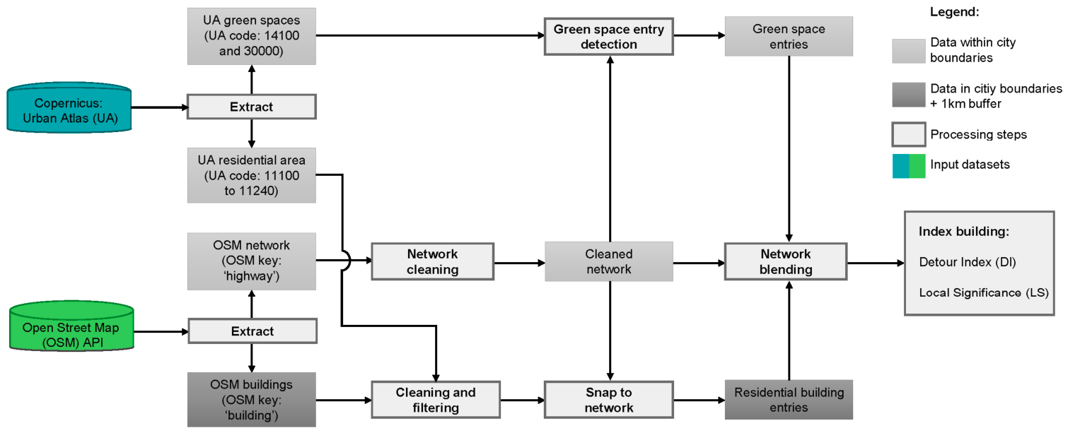
We applied our analysis (Figure 1) to the city of Leipzig while ensuring a reproduction of the approach for other cities in Europe.

3.1. Data Acquisition and Processing

In following our research questions, comparable and open access data on a high resolution is required (for details on data acquisition see Supplementary Materials, Section S1). We used Urban Atlas (UA, version 13 [28]) 2018 and OpenStreetMap [29] as our main data sources. We acquired the OSM data via the OSM API and the R package ‘osmdata’ (version 0.3.0). All analyses were carried out and tested in R 4.1.3 using RStudio version 1.4.1717 and are made available on the GitHub repository www.github.com/blabohm/MA URL (accessed on 4 November 2025).

Street network represents the walkable environment of a city, which connects the entry points of the UGS with those of the residential buildings. To ensure network connectivity and reduce overlap, we cleaned the OSM network [30]. Further information on the pre-processing and cleaning steps can be found in Supplementary Materials, Section S2. The following analysis requires information on a cities’ residential buildings, their entry points and on how many persons inhabit each building. We filtered the OSM ‘building’ polygons for residential buildings. We only kept those OSM buildings whose centroids were contained inside of Urban Atlas residential areas (UA class code 11100–1240). To detect building entries, we first calculated the centroids of each building lying inside the polygon [31]. We snapped the centroids to the closest point on the cleaned street network and assumed the resulting points to be the building entries. To assign each OSM building a reasonable population count, we used a simple area-weighting disaggregation approach [32]. The UA dataset provides information on population mostly on a city block level. We disaggregated this data to the building level by distributing the population proportionally to a building’s base area. This workflow follows the assumption that the building structure, and thus the population per base area inside one city block, is similar. For buildings that were contained inside UA residential polygons that erroneously did not have population values, we used the mean population per square-meter of the corresponding UA residential class in the city. Finally, we filtered the UA data for the classes ‘green urban areas’ (UA class code 14100) and ‘forests’ (UA class code 31000) to ensure that all green spaces that are used in the analysis are publicly accessible. To detect green space entries, we intersected the outline of the UA green spaces with the cleaned network. Furthermore, we applied different buffer sizes to the green space polygons as sensitivity analysis. We used the resulting points as entry points of the green spaces for further analysis. In case a green space did not receive any entry points, we incrementally increased the buffer sizes. In the process of network blending, the entry points of the residential buildings and the UGS (now called ‘nodes’) are being ‘blended’ into the network. During this process, the lines (now called ‘edges’) will be broken at every node location. The node location now represents the new starting/ending points of the newly created edges.

3.2. Analysis

Our first objective is to develop a modeling approach that incorporates the Detour Index (DI) and Local Significance (LS) walkability indices. For computational efficiency, the catchment area around each building, is limited to a network distance of 500 m. Both indices are calculated for each urban green space (UGS) within the city core, including an additional 1 km buffer. To account for maximum walking distance, the DI and LS are computed for residential buildings located within a 500 m network distance between each building entrance and the nearest access point to a UGS. We adopt a modified version of the two indicators proposed by Wolff [16].

Detour Index (DI): The DI measures the presence of barriers within the network by evaluating the efficiency of routes taken by residents to reach the nearest UGS. The DI combines the Euclidean distance, i.e., the direct connection between two points, with the network distance:

$$\mathrm{D}\mathrm{I}={\displaystyle \frac{{\mathrm{D}}_{\mathrm{i},\mathrm{j}}}{{\mathrm{N} \mathrm{D}}_{\mathrm{i},\mathrm{J}}}}$$

(1)

where DI is the Detour Index, D is the Euclidean distance between points i and j, and ND is the network distance between the points i and j. In the case of this analysis, the two points are the entry points of a residential building and the nearest entry point of a UGS. The DI can assume values between 0 and 1. A DI value of 1 represents a straight line between building entry and UGS entry, while a DI value closer to 0 means that the inhabitants of the building have to take a sub-optimal route to the nearest UGS. If one building has access to several UGS within a network distance of 500 m, we decided to use the mean DI value.

Local Significance (LS): LS is commonly used as an indicator of edge importance in network analysis to represent the number of people with access to a given UGS. LS also accounts for the size of an UGS as well as the distance between people’s homes and UGS entries:

$$\mathrm{L}\mathrm{S}={\displaystyle \frac{{\mathrm{P}}_{\mathrm{i}}\ast {\mathrm{A}}_{\mathrm{j}}}{{\mathrm{L}\mathrm{S}}_{\mathrm{i},\mathrm{j}}^2}}$$

(2)

where LS is the Local Significance, P is the population of building i, A is the area of UGS j and ND is the network distance between the entry points of building i and UGS j. This indicator can assume infinite values. A higher population and area, as well as a lower network distance, lead to higher LS values. We attached the LS values to each segment (edge) of the path between building and UGS entries. We summed the LS values of overlapping paths from multiple buildings, leading to higher values on higher frequented edges. A more detailed summary on index building can be found in Supplementary Materials, Section S3.

To demonstrate application possibilities of the indices, we visualized the DI and LS values for the area surrounding the Lene Voigt Park (LVP) in Leipzig. The city of Leipzig is the largest city in Saxony, Germany. After a massive population loss in the 1990s, the city faced a major regrowth since 2012. Rising population numbers led to increased pressure on the open spaces of the city. The LVP was a former train station area and has been out of use since 1942. In the 2000s, it was converted to a public park and has been fully open since 2004 [33]. Its diverse history and the population dynamic make the LVP an interesting test case for the demonstration of our results. Since LS values tend to grow exponentially, we chose to use a logarithmic scale for visualization.

The final objective was to apply the two developed indices to demonstrate potential use cases for urban planners. To assess the impact of changes in model parameters, we tested three scenarios and evaluated the resulting changes in index values relative to the baseline model.

Alternative 1—Unlimited access: In the first scenario, we demonstrate how the LS and DI indicators change if all barriers obstructing access to the LVP are removed. To model unlimited access, we distributed hypothetical entry points every 5 m on the network surrounding the LVP and applied the walkability indices to the changed conditions.

Alternative 2—Green space development: In the second scenario, we investigated the impact of development of the green spaces surrounding the LVP to residential buildings. We assumed the following green spaces in the north of the LVP to be developed to high-density residential buildings: Reudnitzer Park, Staphaniplatz, and the green space between Täubchenweg, Perthesstraße and Gerichtsweg. To implement this scenario, we converted the former green space entry points to building entries. We multiplied the size of the parks by the 95th percentile of the population per square meter value derived from the Urban Atlas high-density residential class in the surrounding two kilometers. We distributed the outcome uniformly across the former green space entries and applied the two walkability indices.

Alternative 3—Population increase: In the third scenario, we modeled a population increase in the residential areas surrounding the LVP. For each residential building in a distance of 2 km to the LVP, we increased the population value to the 95th percentile of the respective Urban Atlas residential class. We then applied the DI and LS indices to the changed conditions.

Finally, and as urbanization usually combines versions of the three alternatives outlined above, we applied the changes from the unlimited access, green space development, and population increase scenarios in a single ensemble model.

4. Results

4.1. Applying Walkability Indices

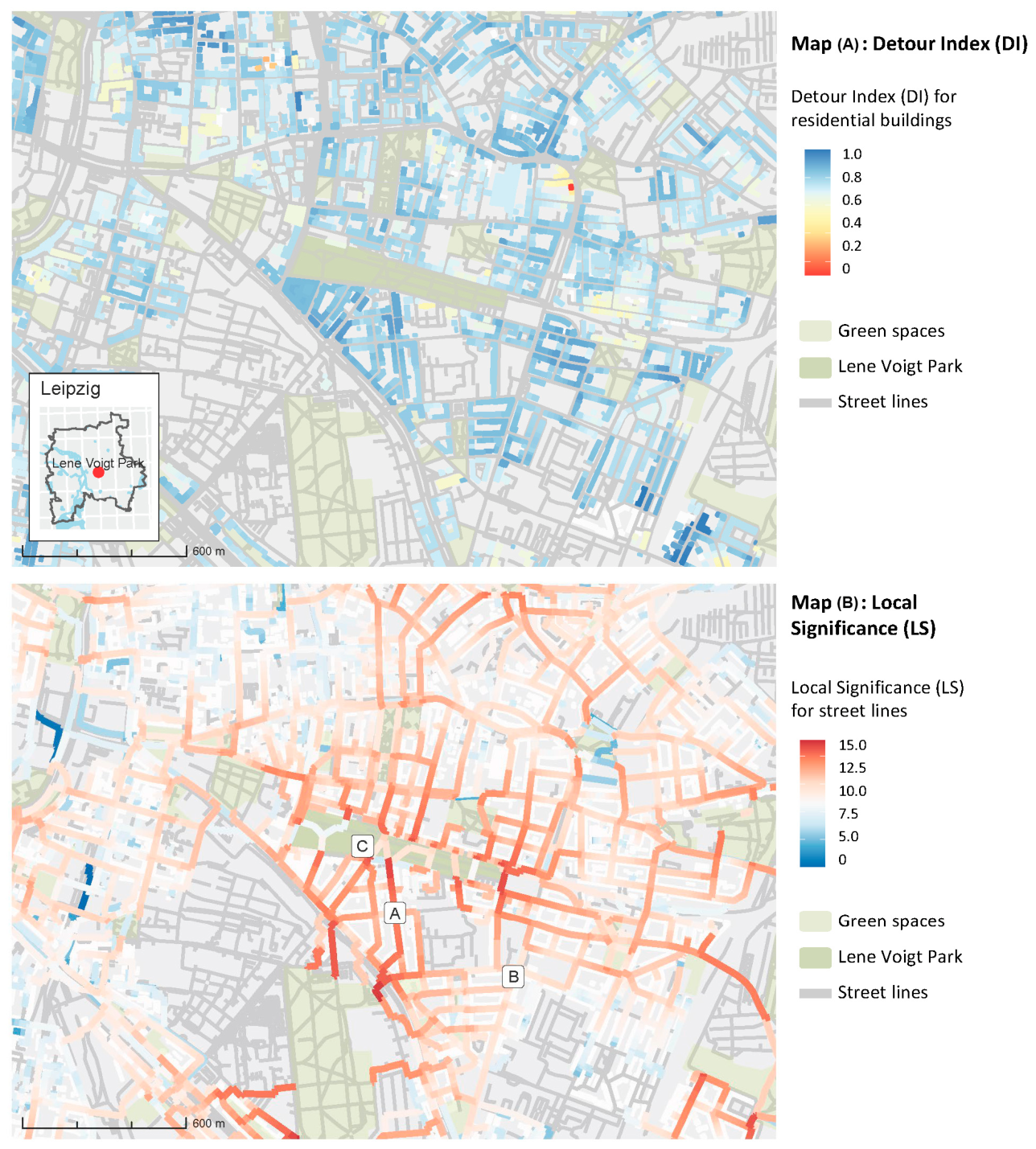
In this section, we present the results of applying the two walkability indices to the test case, the Lene Voigt Park (LVP) in Leipzig, Germany. Figure 2A displays the Detour Index (DI) and illustrates that high DI values can be found at buildings that are located at streets which lead directly to a green space entry. Along these streets there are straight formations of buildings with high DI values as can be seen in the south of the LVP. In contrast, low DI values cluster in areas where larger detours have to be taken to reach an UGS. Such areas can be found in the northeast of the map. Furthermore, we can observe low DI values at buildings that are close to several UGS but whose routes towards one or more UGS are inefficient. Some buildings that are directly adjacent to one UGS, but have to take small detours to the nearest green space entry point, also show low DI values. Lastly, we see that there are buildings close to UGS with high DI values but that have to cross larger streets or other obstacles to reach the green space entry point.

Figure 2B displays the Local Significance (LS) values. Due to the high density of green spaces and residential buildings in the area, an overall high level of LS values can be observed. In general, LS values tend to grow towards green space entry points—i.e., higher LS values can be observed in closer distance to UGS. Due to the cumulative nature of our LS representation, this effect symbolizes street segments with the potential for overcrowding. Furthermore, high LS values are associated with direct connections between parks and residential buildings. The highest LS values can be found at park entries adjacent to streets which connect UGS to areas with a high population, indicating street segments that are highly visited for routes towards a UGS. The eastern part of the LVP close to marker B on the map is a good example of this (see Figure 2B). Here, we find high LS values at those parts of the streets that lead to the residential areas in the north, east and south-east. Furthermore, the connecting street between LVP to the next larger park in the south, the Friedenspark, displays high LS values (marker A). On the other hand, we can make out lower LS values at streets with residential buildings that are close to the cut-off threshold of a 500 m distance to the nearest green space. For example, in the southeast of the map, in many streets, the blue shade is getting brighter with each street segment until it switches over to red shades. With each building entry, more inhabitants are expected to take these routes towards the nearest green space. This increases the LS values of the street segments.

4.2. Demonstrating the Planning Relevance of Walkability Indices

In this section, we demonstrate how local planners can apply the two walkability indicators introduced above. To this end, we revisit the LVP example presented in Section 4.1 and explore three alternative scenarios in which the built environment is modified to reflect common planning interventions. In each scenario, one of the key variables used to calculate DI and LS is adjusted. In the first alternative, “unlimited access,” we assume that the LVP is accessible from all sides of the park. In the second alternative, “densification,” several UGS located north of the LVP are replaced with residential buildings. In the third alternative, “population growth,” we assume an increase in the number of residents in the area surrounding the LVP.

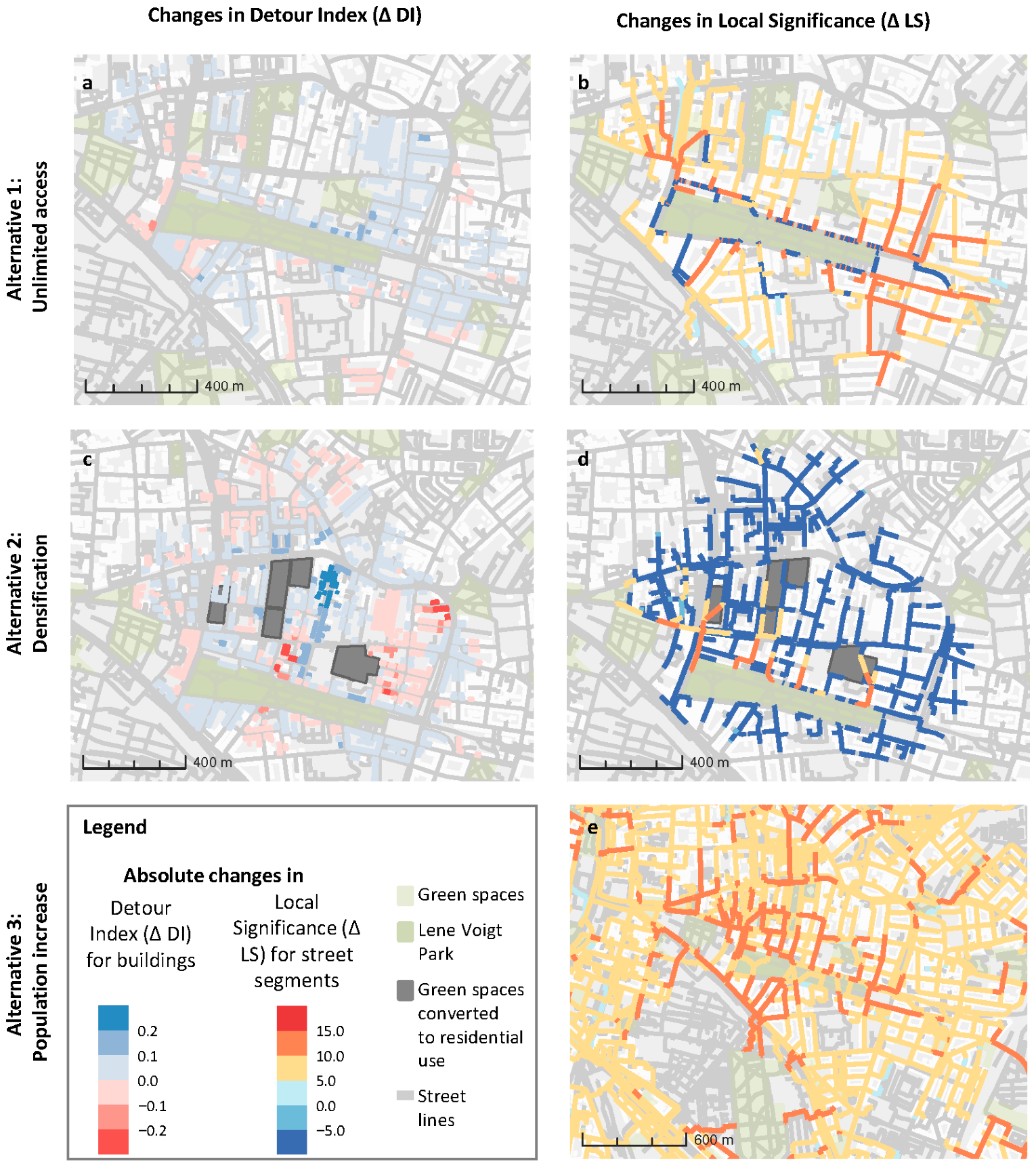
Alternative 1—Unlimited access: In the first alternative, we demonstrate how the DI and LS indicators change if all barriers obstructing access to the Lene Voigt Park (LVP) were to be removed. We do so by assuming a park entry every 5 m on the network surrounding LVP. As can be seen from Figure 3a, the routes towards the nearest UGS have become more direct as illustrated by increasing DI values (delta DI ~ 0.1). This in turn represents a facilitated access to the nearest UGS for the residents of the building. Moreover, Figure 3b displays that in this alternative, LS values decrease on all streets that are adjacent to the LVP, while in greater proximity from the park, LS values increase. Thus, according to our model, removing the barriers along the edges of the LVP would result in less crowded streets surrounding the park, which may be a desirable effect for city planners. On the other hand, more people could reach the LVP, increasing the overall amount of people traveling through the network and towards the park. Accordingly, removing entry barriers could also be a pull factor for a UGS when providing unlimited access. We filtered out any delta DI values that were smaller than +/−0.05 to place emphasis on the more significant changes. It appears as though the change in DI values is mostly limited to buildings that are either very close to the park or that were not reachable before, but are now inside the threshold network distance of 500 m.

A few buildings adjacent to the eastern part of the LVP express an increase larger than 10; the larger area to the northeast and smaller areas to the east and south of the center of the LVP show a minor increase in DI values. These buildings’ residents may now be able to take a more efficient trajectory towards the LVP. In the northwest of the map, we see a cluster of buildings that seem to have gained access to the LVP via a direct path, which increased their DI values. Contrary, in the southeast there are a couple of buildings that have gained access as well, but on a less direct path. For these buildings the DI values decrease, meaning the average trajectories towards the nearest UGS have become less efficient.

Alternative 2—Densification: In the second alternative we intended to see how the indices behave if the green spaces in the city blocks north of the LVP were to be developed into residential areas. To apply these changes, we switched the former park entries into building entries and distributed a population among them according to the former park’s size. In Figure 3c we see DI values mostly increasing in the area. The buildings along the street that lead from the center of the LVP north especially experience a substantial DI increase. Again, a higher DI means more efficient routes to the nearest parks. Some areas in the east and north of the map express a decrease in DI values, representing less efficient trajectories towards the nearest UGS. In the south and west of the LVP we observe a mixed picture of minor de- and increases. The five green spaces that we intended to change into residential areas are comparatively small and, thus, “hard to reach”. Taking them out of the equation seems to leave the surrounding buildings with more efficient trajectories towards the larger parks. Furthermore, Figure 3d shows that overall, most of the LS values appear to decrease substantially. Since the UGS disappeared, the trajectories of the people that traveled to them have disappeared as well, leading to decreased LS. Only on the paths connecting the newly built residential areas to the LVP and the former Johannes cemetery in the west can we see a substantial increase in LS values. Overall, the reduction in the number of parks in the area seems to have a larger effect on the LS index than the increase in population due to the newly “constructed” residential buildings.

Alternative 3—Population increase: The third alternative is designed to demonstrate how a population increase would affect the DI and LS indices. In this alternative, we assumed for each residential building a population increase to the 95th percentile of the population per area. Since we did not change the locations of any green spaces or building entries, the DI did not change, either. As we can see in Figure 3e, the delta LS is positive in the entire area. In contrast to the other alternatives, changes are now scattered across the entire map, since we also applied the population growth to all buildings in the area. In this alternative, we see a similar pattern as in the basic LS map (see Figure 2). LS tends to grow larger the closer a street is to one of the large parks, especially along those streets where the population flows from multiple areas combine on their way towards the UGS. For example, we can observe high LS values between the LVP and the Friedenspark in the south of LVP. The further away a street is from the larger parks, the lower the increase in LS. Close to LVP we now observe a large cluster with high LS values in the west. If we have a look at the population data that is attached to the residential buildings, we can see that the area in the northwest of the LVP has several buildings with a very high population. Most of these buildings can reach the LVP only via the entry point at the northwest, which causes the high LS values in this area.

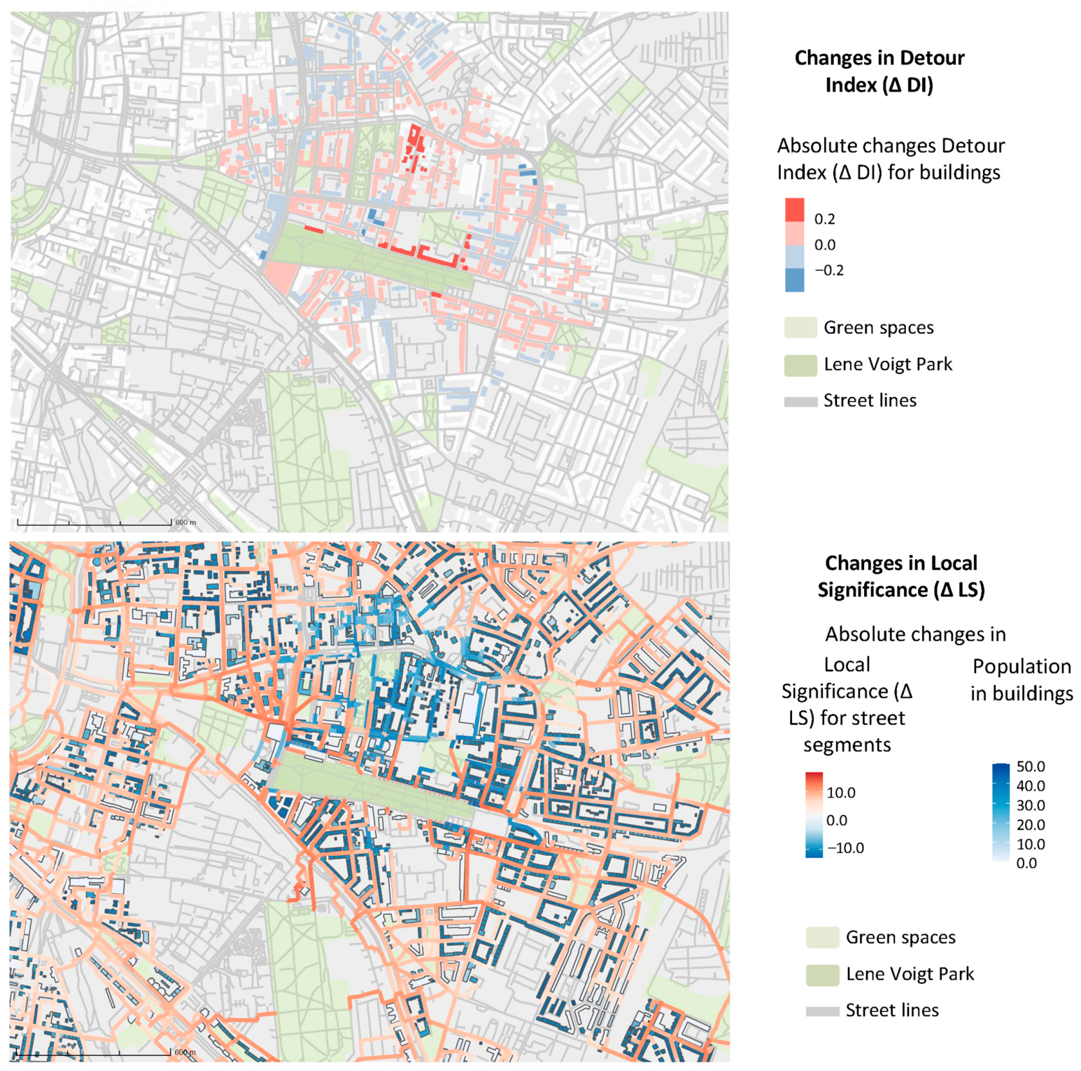
Ensemble model

As urbanization usually combines versions of the three alternatives outlined above, we applied all the changes and translated this into an ensembled model. The joint effects of removing barriers, developing the green space in the north and a population increase can be seen in Figure 4. Change in DI is restricted to those buildings that either reached one of the now developed green spaces before or that can reach the LVP through one of the new entry points. In the fourth alternative we can still see an overall increase in the DI from removing the small and hard-to-reach green space in the north of the LVP. Also, the mixed effects from removing the entry barriers to the LVP can still be observed in the south or the northwest of the LVP. For both LS and DI, the overall changes in this alternative appear more gradual than, for example, in the densification scenario, and are most apparent where we apply intense constructional changes. Figure 4 further shows that the change in the LS index is mostly influenced by the population increase and the green space development alternatives. Due to the population increase, we see a general increase in LS, except for those streets that experience a decrease in LS due to the removed green spaces. This makes the changes in LS appear more diffuse than in the other alternatives. Similar to the population increase alternative, we see a large area with a high LS increase in the northwest of the LVP. In this alternative we can simultaneously observe the effects of the population increase and the unlimited access alternatives. The nearest entry point for the area with the high population residential buildings in the northwest has been shifted to the northernmost corner of the LVP in contrast to the third alternative.

5. Discussion

In this paper, we present a modeling approach that applies two walkability indices: Detour Index (DI) and Local Significance (LS). These indices are based on publicly available data and software tools. We also demonstrated the potential applications of the LS and DI indices for city planners using an urban park, Lene Voigt Park in Leipzig, as a test case. In a consistent methodological reflection, we report on the advantages and limitations of the applied procedure.

Usefulness of the proxies

In a previous study, Wolff [16] mapped LS using colored straight lines that connected residential areas directly to the respective UGS. This representation of the index provides an overview of potential overcrowding in individual UGS and the strength of expected recreational flows towards green spaces. By plotting LS in a cumulative way on individual street segments, we achieve an even more targeted representation of the flows. In an individual city, areas of high use intensity with potential for overcrowding can be identified at a glance as red clusters around the UGS in question. Consequently, researchers and city planners can use our results to identify potential overcrowding that could restrict access to a specific UGS at individual street segments or green space entry points and display the corresponding Service-Connecting Area (SCA) crowding effects [17,21].

Our representation of the DI enables users to see at first glance which buildings have direct access to UGS, and whether they can reach a UGS in an unobstructed manner. The index provides an estimation of potential detours people have to take in order to reach a UGS: the closer the route towards the UGS is to a straight line, the higher is the DI, suggesting a better accessibility [18]. Consequently, this index is a good proxy showing discontinuous accessibility options of people without suggesting an artificial dichotomous differentiation between having and not having access, such as what was applied in various previous studies [8,11]. In some cases, low DI values may occur in close proximity to UGS as an artifact of small Euclidean and network distances values. In these cases, a minor difference can lead to a low DI value even though the overall traveling distance to the next green space entry is relatively small. Nonetheless, both walkability indices may be combined with local demographic, socioeconomic or environmental data, which can open up further opportunities for city planners. For example, intersections with data on air pollution or heat exposure along the street network might help in the decision process for intervention [8].

Planning relevance

To demonstrate the potential applications of the two walkability indices for city planners and researchers, we implemented the LS and DI in three alternatives for our model case: the Lene Voigt Park (LVP) in Leipzig. Generally speaking, an increase in a building’s DI value is desirable because residents have a more efficient—or more direct—route to a UGS. Consequently, people may be encouraged to visit the UGS more frequently and enjoy the benefits of physical exercise and being in nature, which is in line with previous studies [4]. In contrast, an increase in the LS value of a street segment is usually considered negative. If no major changes to the built environment have been implemented, an increase in LS indicates that more people are traveling through the same network, resulting in more crowded streets, which could negatively impact UGS accessibility. The results suggest that LS and DI are useful tools for assessing urban green space demand. They provide a framework for evaluating how planning interventions may influence green and blue infrastructure before implementation, allowing planners to anticipate shifts in both supply and demand. Moreover, the combined application of LS and DI highlights their potential to support integrated planning of street networks, residential development, and green and blue infrastructure. This integrated perspective can foster coordination across planning departments and help mitigate unintended trade-offs.

In the first alternative, we modeled unlimited access to the LVP by adding green space entry points every five meters on the outline of the park. At the immediate surrounding of the LVP, the LS index behaved as expected. Here, removing the entry barriers resulted in a decrease in the index, representing less crowding taking place, which is desirable for urban planners, as it might alleviate the effects of overcrowding. Nonetheless, the implementation of the unlimited access alternative showed ambiguous effects. A UGS with less barriers might be more attractive, and thus pull more people from the surrounding residential areas, resulting in more traffic in the remaining network and a higher overall visitation of the park itself. The DI values of most of the residential buildings express only minor changes. The small changes in the network distance that occur when the nearest green space entry point is shifted do not carry as much weight if network and Euclidean distance values are larger. In contrast, close to the LVP, the small changes have a larger effect on the DI values, resulting mostly in substantial increases in the index. The contradicting effects on the DI values of those buildings that have ‘gained’ access through removal of barriers show that considering the DI alone might not yield a full picture on UGS accessibility.

The LS index reacts strongly to the changes that we have applied to the built-up structure in the area during the second alternative, densification. Replacing the UGS with residential areas would cause the absolute number of people that use the network to increase. Our representation of the LS reacted contra-intuitively to the changes, though. Removing the UGS reduced the overall number of trajectories modeled, which in turn decreased the index values for most of the network. The only values that did increase at those street segments were the ones that lead from the converted UGS to the remaining ones. The strong LS decrease in most of the network, as well as its evenly strong increase at certain streets, highlight the importance of the UGS that were changed into residential buildings: many nearby residents rely on these spaces for recreation; converting them and increasing population density would further crowd the remaining UGS. Furthermore, the second alternative has shown that taking UGS that prove harder to reach out of the equation can increase the DI. An increasing DI itself means that residents travel along efficient trajectories towards UGS. Thus, only considering DI values might implicate that the green space accessibility for residents improves when green spaces are converted to build-up. Since we are only looking at distances, the index lacks to account for an in- or decrease in the number of alternative green spaces.

The modeled population increase in alternative three resulted in a general increase in LS values in the entire area. Where the population flows from multiple areas combine on their way towards the UGS we can visualize potential crowding effects that might occur if population-increasing trends tend to continue [34]. These results also enrich different, more areal-based approaches on different density patterns emerging from the constellation of population trajectories and built-up area.

Finally, by considering all changes together, we can observe the complex interactions between the built environment, population and UGS. At first glance, the increase in population seems to dominate the other changes. However, a closer look reveals the effects of converting green spaces into residential areas and providing unlimited access to the LVP. Overall, changes to the built environment have a higher impact on the movement of residents towards UGS than population growth. An increase in urban dwellers adds to the crowding effects caused by other changes, such as densification.

Method reflection

There are several factors that limit our approach. The quality of both indices depends on the quality of the data they are built on. Errors in the UA or OSM datasets may propagate from the preparation of the data to the building of the index and multiply along the way. Both indices only account for the fastest routes from residential buildings to UGS in a walking distance of 500 m, given the underlying network. People might choose their routes towards UGS based on different factors than pure distance. Elements of attractiveness such as equipment, cultural events, etc., might encourage people to approach UGS in greater distances [24,35]. Our application of the LS and the DI fails to account for obstacles people have to overcome on their ways to the nearest UGS like traffic lights, large streets or other physical barriers [36]. Another important point is that, by using the Urban Atlas classes Green urban areas and Forests (codes 14100 and 31000), we have only accounted for publicly accessible green spaces. Furthermore, the role of private or residential green cannot be underestimated, since a high share of residents might prefer the use of their private green space over publicly accessible ones [37,38]. This effect might cause LS values to overestimate the flow of people from their homes to UGS. By leaving private green out of the equation, we cannot account for institutional barriers of accessibility [24]. However, combining the DI or LS with such measures could allow for inferences to be made at a per-building level instead of a UGS level. This would enable more accurate quantitative and qualitative assessments than before [39]. Lastly, our study did not address how people reach UGS by means of public transport, private motorized transport or cycling. Including public transport in the model could help to remove further uncertainties in future research.

A further limitation of our approach concerns the lack of empirical validation against observed patterns of actual use. While the indices presented here aim to approximate potential flows and accessibility conditions, they do not capture how residents truly perceive and utilize urban green spaces in practice. Integrating observational data or interview-based insights could help assess the degree to which the modeled accessibility patterns correspond to real-world behavior. Such a comparison would also provide a basis for evaluating the consistency between the analytical model and the current state of use, thereby offering indications on how reliably simulated scenarios may translate into actual outcomes. However, incorporating these micro-level factors remains challenging, as many of them are difficult to quantify and were beyond the scope of this study. Future research should therefore focus on model calibration and validation, particularly by linking computational results with empirical evidence, in order to improve the robustness and predictive capacity of the approach.

6. Conclusions

This study introduces a computational, network-based approach to analyzing urban walkability in relation to urban green spaces (UGS), with a particular focus on the service-connecting areas (SCA) between residential demand and green space supply. By combining the Detour Index (DI) and Local Significance (LS), the study shifts attention from purely areal or distance-based accessibility measures towards the structure and use of the urban network itself.

The main contribution lies in integrating proximity, provision, and population pressure within a unified, high-resolution modeling framework. Unlike conventional approaches based on fixed buffers or aggregated indicators, the proposed method captures accessibility conditions and potential use patterns along specific street segments. This enables the identification not only of whether green spaces are accessible, but also of how accessibility is spatially organized and where potential mismatches between supply and demand may occur within the urban fabric.

From a planning perspective, the indices provide a practical tool for exploring the spatial implications of different urban development scenarios. By modeling changes in access, land use, and population distribution, the framework supports assessments of how interventions may influence movement patterns, potential crowding, and local accessibility gradients. In doing so, the approach helps bridge analytical modeling and applied urban planning through interpretable indicators linked to concrete spatial decisions.

At the same time, the study remains exploratory. Although use of open and comparable datasets suggests potential transferability to other urban contexts, this has not yet been empirically validated. Likewise, the indices approximate potential accessibility and flows, but do not account for behavioral, perceptual, or institutional factors influencing actual use.

Future research should therefore focus on validating and refining the framework through empirical data integration and improved model calibration. Particular attention should be given to accounting for multiple accessible green spaces, qualitative dimensions of accessibility, and observed use behavior. Strengthening the empirical basis of the model will be essential for accessing how closely simulated patterns reflect real-world dynamics and for increasing its relevance to planning practice.

Overall, this study contributes to a more nuanced understanding of urban green space accessibility by emphasizing the networked interactions between people, infrastructure, and green spaces. It highlights the importance of viewing the urban fabric as a dynamic system rather than a static distribution of resources, providing a basis for more differentiated analyses of accessibility in rapidly changing urban environments.

References

1. Elmqvist, T.; Andersson, E.; McPhearson, T.; Bai, X.; Bettencourt, L.; Brondizio, E.; Colding, J.; Daily, G.; Folke, C.; Grimm, N.; et al. Urbanization in and for the anthropocene. npj Urban Sustain. 2021, 1, 6. [Google Scholar] [CrossRef] [Scilit]
2. UN. World Urbanization Prospects: The 2018 Revision; United Nations: New York, NY, USA, 2019. [Google Scholar]
3. Fisher, B.; Turner, R.K.; Morling, P. Defining and classifying ecosystem services for decision making. Ecol. Econ. 2009, 68, 643–653. [Google Scholar] [CrossRef] [Scilit]
4. Kabisch, N.; Kraemer, R.; Masztalerz, O.; Hemmerling, J.; Püffel, C.; Haase, D. Impact of summer heat on urban park visitation, perceived health and ecosystem service appreciation. Urban For. Urban Green. 2021, 60, 127058. [Google Scholar] [CrossRef] [Scilit]
5. Poelman, H. A Walk to the Park? Assessing Access to Green Areas in Europe’s Cities Update Using Completed Copernicus Urban Atlas Data. 2018. Available online: https://ec.europa.eu/regional_policy/en/information/publications/working-papers/2018/a-walk-to-the-park-assessing-access-to-green-areas-in-europe-s-cities (accessed on 17 April 2025).
6. UN. Transforming our world: The 2030 agenda for sustainable development. In A New Era in Global Health; Rosa, W., Ed.; Springer Publishing Company LLC: New York, NY, USA, 2017. [Google Scholar]
7. Wolff, M.; Haase, D. Mediating sustainability and liveability—Turning points of green space supply in european cities. Front. Environ. Sci. 2019, 7, 61. [Google Scholar] [CrossRef] [Scilit]
8. Larondelle, N.; Haase, D. Urban ecosystem services assessment along a rural–urban gradient: A cross-analysis of European cities. Ecol. Indic. 2013, 29, 179–190. [Google Scholar] [CrossRef] [Scilit]
9. Syrbe, R.-U.; Walz, U. Spatial indicators for the assessment of ecosystem services: Providing, benefiting and connecting areas and landscape metrics. Ecol. Indic. 2012, 21, 80–88. [Google Scholar] [CrossRef] [Scilit]
10. Richardson, E.A.; Pearce, J.; Mitchell, R.; Kingham, S. Role of physical activity in the relationship between urban green space and health. Public Health 2013, 127, 318–324. [Google Scholar] [CrossRef] [Scilit] [PubMed]
11. Kabisch, N.; Strohbach, M.; Haase, D.; Kronenberg, J. Urban green space availability in European cities. Ecol. Indic. 2016, 70, 586–596. [Google Scholar] [CrossRef] [Scilit]
12. Moseley, D.; Marzano, M.; Chetcuti, J.; Watts, K. Green networks for people: Application of a functional approach to support the planning and management of greenspace. Landsc. Urban Plan. 2013, 116, 1–12. [Google Scholar] [CrossRef] [Scilit]
13. Sander, H.A.; Ghosh, D.; van Riper, D.; Manson, S.M. How do you measure distance in spatial models? An example using open-space valuation. Environ. Plan. B Plan. Des. 2010, 37, 874–894. [Google Scholar] [CrossRef] [Scilit]
14. Pafi, M.; Siragusa, A.; Ferri, S.; Halkia, S. Measuring the Accessibility of Urban Green Areas: A Comparison of the Green ESM with Other Datasets in Four European Cities; JRC102525; Publications Office of the European Union: Luxembourg, 2016. [Google Scholar]
15. Luo, W.; Whippo, T. Variable catchment sizes for the two-step floating catchment area (2sfca) method. Health Place 2012, 18, 789–795. [Google Scholar] [CrossRef] [Scilit]
16. Wolff, M. Taking one step further—Advancing the measurement of green and blue area accessibility using spatial network analysis. Ecol. Indic. 2021, 126, 107665. [Google Scholar] [CrossRef] [Scilit]
17. Barthelemy, M. Morphogenesis of Spatial Networks; Springer: Cham, Switzerland, 2018. [Google Scholar]
18. Esch, T.; Marconcini, M.; Marmanis, D.; Zeidler, J.; Elsayed, S.; Metz, A.; Müller, A.; Dech, S. Dimensioning urbanization—An advanced procedure for characterizing human settlement properties and patterns using spatial network analysis. Appl. Geogr. 2014, 55, 212–228. [Google Scholar] [CrossRef] [Scilit]
19. Syrbe, R.-U.; Grunewald, K. Ecosystem service supply and demand—The challenge to balance spatial mismatches. Int. J. Biodivers. Sci. Ecosyst. Serv. Manag. 2017, 13, 148–161. [Google Scholar] [CrossRef] [Scilit]
20. Higgs, G.; Fry, R.; Langford, M. Investigating the implications of using alternative gis-based techniques to measure accessibility to green space. Environ. Plan. B Plan. Des. 2012, 39, 326–343. [Google Scholar] [CrossRef] [Scilit]
21. Dworczyk, C.; Burkhard, B. Conceptualising the demand for ecosystem services—An adapted spatial-structural approach. One Ecosyst. 2021, 6, e65966. [Google Scholar] [CrossRef] [Scilit]
22. Feltynowski, M.; Kronenberg, J.; Bergier, T.; Kabisch, N.; Laszkiewicz, E.; Strohbach, M.W. Challenges of urban green space management in the face of using inadequate data. Urban For. Urban Green. 2018, 31, 56–66. [Google Scholar] [CrossRef] [Scilit]
23. Baro, F.; Palomo, I.; Zulian, G.; Vizcaino, P.; Haase, D.; Gómez-Baggethun, E. Mapping ecosystem service capacity, flow and demand for landscape and urban planning: A case study in the barcelona metropolitan region. Land Use Policy 2016, 57, 405–417. [Google Scholar] [CrossRef] [Scilit]
24. Biernacka, M.; Kronenberg, J. Urban green space availability, accessibility and attractiveness, and the delivery of ecosystem services. Cities Environ. (CATE) 2019, 12, 1–17. [Google Scholar]
25. Ibes, D.C. A multi-dimensional classification and equity analysis of an urban park system: A novel methodology and case study application. Landsc. Urban Plan. 2015, 137, 122–137. [Google Scholar] [CrossRef] [Scilit]
26. Wang, D.; Brown, G.; Liu, Y. The physical and non-physical factors that influence perceived access to urban parks. Landsc. Urban Plan. 2015, 133, 53–66. [Google Scholar] [CrossRef] [Scilit]
27. Kimpton, A. A spatial analytic approach for classifying greenspace and comparing greenspace social equity. Appl. Geogr. 2017, 82, 129–142. [Google Scholar] [CrossRef] [Scilit]
28. European Union. Mapping Guide v6.2 for a European Urban Atlas. 2020. Available online: https://land.copernicus.eu/en/products/urban-atlas (accessed on 12 September 2025).
29. OpenStreetMap Contributors. OpenStreetMap. 2022. Available online: https://download.geofabrik.de/ (accessed on 20 September 2025).
30. van der Meer, L.; Lovelace, R.; Abad, L. Spatial Networks in R with sf and Tidygraph. 2019. Available online: https://r-spatial.org/r/2019/09/26/spatial-networks.html (accessed on 22 September 2025).
31. Pebesma, E. Simple Features for R [R Package sf Version 1.0-8]. Comprehensive R Archive Network (CRAN). 2022. Available online: https://cran.r-project.org/web/packages/sf/index.html (accessed on 15 October 2025).
32. Li, T.; Pullar, D.; Corcoran, J.; Stimson, R. A comparison of spatial disaggregation techniques as applied to population estimation for south east queensland (seq), australia. Appl. GIS 2007, 3, 1–16. [Google Scholar] [CrossRef] [Scilit]
33. Stadt-Leipzig. Lene-Voigt-Park. 2022. Available online: https://www.leipzig.de/leben-in-leipzig/natur-und-umwelt/parks-waelder-und-friedhoefe/parks-und-gruenanlagen/lene-voigt-park (accessed on 3 October 2025).
34. Cortinovis, C.; Geneletti, D.; Haase, D. Higher immigration and lower land take rates are driving a new densification wave in european cities. npj Urban Sustain. 2022, 2, 19. [Google Scholar] [CrossRef] [Scilit]
35. Dickinson, D.C.; Hobbs, R.J. Cultural ecosystem services: Characteristics, challenges and lessons for urban green space research. Ecosyst. Serv. 2017, 25, 179–194. [Google Scholar] [CrossRef] [Scilit]
36. Barber, A.; Haase, D.; Wolff, M. Permeability of the city—Physical barriers of and in urban green spaces in the city of halle, germany. Ecol. Indic. 2021, 125, 107555. [Google Scholar] [CrossRef] [Scilit]
37. Chiesura, A. The role of urban parks for the sustainable city. Landsc. Urban Plan. 2004, 68, 129–138. [Google Scholar] [CrossRef] [Scilit]
38. Säumel, I.; Hogrefe, J.; Battisti, L.; Wachtel, T.; Larcher, F. The healthy green living room at one’s doorstep? use and perception of residential greenery in Berlin, Germany. Urban For. Urban Green. 2021, 58, 126949. [Google Scholar] [CrossRef] [Scilit]
39. Biernacka, M.; Kronenberg, J.; Laszkiewicz, E. An integrated system of monitoring the availability, accessibility and attractiveness of urban parks and green squares. Appl. Geogr. 2020, 116, 102152. [Google Scholar] [CrossRef] [Scilit]
Figure 1. Workflow of data acquisition, processing and analysis.
Urbansci 10 00313 g001
Figure 2. Results of the walkability modeling for a demonstration area in the city of Leipzig. Map (A): Detour Index (DI) as an index of physical barriers. The building colors represent average DI calculated for all green spaces in a network distance of 500 m from a building. The darker blue the color of a building is, the closer to 1 the DI value, the more direct can its residents travel to the closest green spaces. The opposite is the case if the color tends towards orange. Map (B): Local Significance (LS) for network edges (a.k.a. streets and paths). The network colors depict the cumulative LS. A higher LS value is depicted by a darker red color, representing (i.) more people taking this path, (ii.) the people taking this path are living in closer proximity to the green space, and/or (iii.) the path is leading to a larger green space. Since the LS values are cumulative, a higher value might also mean more paths from different buildings overlapping (See Supplementary Materials, Section S3, for further information). The following examples are referred to in the running text: A = Josephinenstraße; B = Riebeckstraße; C = Leve-Voigt-Park.
Urbansci 10 00313 g002
Figure 3. Changes in values for Detour Index (maps (a,c)) and Local Significance (maps (b,d,e)) according to three planning alternatives (unlimited access, densification, population increase. Higher DI means that the trajectories from a building to the nearest UGS entry have become more efficient. Increasing LS values depict street segments that are more visited.
Urbansci 10 00313 g003
Figure 4. Ensemble model output combining changes of Detour Index (top map) and Local Significance (bottom map) in three alternatives (unlimited access, densification, population increase, see Figure 3).
Urbansci 10 00313 g004
Disclaimer/Publisher’s Note: The statements, opinions and data contained in all publications are solely those of the individual author(s) and contributor(s) and not of MDPI and/or the editor(s). MDPI and/or the editor(s) disclaim responsibility for any injury to people or property resulting from any ideas, methods, instructions or products referred to in the content.