The Spatial Data Generating Process Matters: Re-Evaluating Socio-Economic and Demographic Drivers of Environmental Justice of Urban Tree Ecosystem Services in Two Mediterranean Cities

Abstract

To advance the Sustainable Development Goals, it is essential to correct imbalances in how the benefits of urban trees are distributed across different demographic and socioeconomic groups. Environmental justice studies have frequently overlooked assumptions regarding the data-generating process and have not considered spatial confounding. This oversight potentially misestimates patterns of inequity. This study evaluates the sensitivity of inequity to model assumptions using urban tree inventories from Málaga and Sevilla and Bayesian hierarchical models. City-level differences dominated the inequity patterns, and model specification influenced the magnitude, precision, and credibility of estimated effects, though directionality remained consistent. Patterns were highly consistent across the four ecosystem services, indicating that model assumptions affected all services equivalently. Málaga and Seville exhibited divergent inequity patterns, indicating that local urban context mediates these relationships. In Seville, inequity patterns were inconsistent with the luxury hypothesis and occurred primarily across age-based demographic strata, whereas in Málaga they manifested predominantly along ethnicity, with weaker evidence of income inequities. We advocate for explicitly modeling spatial data-generating processes and comparing conventional versus confounding-mitigated approaches. This city-specific rigor is essential for urban planners to prevent resource misallocation, ensuring that tree-planting strategies address genuine inequities rather than methodological biases.

1. Introduction

Urban thermal stress is accelerating dramatically across the twenty-first century [1,2]. The mortality toll from heat exposure has reached catastrophic proportions, with three particularly severe heat episodes in Europe alone claiming approximately 200,000 lives [3,4,5]. Projected urban thermal conditions reveal an intensifying trajectory through interconnected physical mechanisms: expansion of urban heat island effects [6,7], shifts in heatwave regimes characterized by increased frequency, magnitude, duration, and geographic extent [8,9,10], and amplification through synergistic coupling between localized heat islands and regional extreme heat episodes [11].

Urban environmental degradation encompasses hazards extending well beyond thermal stress, with air quality deterioration and flood hazards representing pressing threats to population health. In 2021, air pollution accounted for an estimated 8.08 million deaths (range: 6.71–9.48 million), with nearly 97% attributable to fine particulate exposure [12]. Although there was a 33.7% decline in European PM_2.5 pollution between 1990 and 2019, this environmental hazard still resulted in 368,006 deaths in 2019 [13]. Worldwide, approximately 1.81 billion individuals (23% of all inhabitants) live in areas directly vulnerable to centennial flood hazards [14]. Climate-driven intensification of precipitation extremes and accelerating sea-level rise are projected to substantially compound the severity, duration, and recurrence of flood disasters [15].

These threats gain heightened significance with accelerating urbanization. Current demographic patterns show that 57.7% of the global population resides in urban areas, with projections indicating 67.9% by 2050 [16]. This urbanization trend, coupled with aging population structures [17], makes the urgent development of adaptive frameworks for urban resilience necessary. Importantly, low-income and marginalized communities experience disproportionately higher exposure to multiple stressors, including air pollution [18,19], flood risk [20], and heat intensity [21,22,23,24]. These inequitable risks pose significant obstacles to achieving the Sustainable Development Goals (SDGs), particularly SDG 3 (Good Health and Well-being), SDG 10 (Reduced Inequalities), and SDG 11 (Sustainable Cities and Communities) [25], underscoring the need for integrated adaptation and mitigation strategies in urban environmental management.

Extensive research has identified numerous strategies for enhancing urban livability [26,27,28,29,30], with urban trees emerging as a particularly promising solution for mitigating multiple environmental challenges through ecosystem services (ES) provision [31,32,33,34,35]. However, extensive evidence from systematic reviews and meta-analyses consistently demonstrates that the spatial distribution of urban trees and canopy cover is inequitable across socioeconomic and demographic strata within cities [24,36,37,38,39,40,41,42,43]. Although a well-established correlation exists between total ES provision and canopy cover, the generation and supply of these services depend largely on the functional traits of urban trees [44,45,46]. As a result, findings in environmental justice research often diverge when relying on tree canopy as a stand-in rather than measuring ES delivery itself. This highlights why directly quantifying ES is crucial [47,48,49]. Reflecting this necessity, recent studies have increasingly prioritized the direct measurement of these services [50,51,52]. Recent literature on environmental justice emphasizes equitable access to and distribution of ES across socioeconomic and demographic strata within cities. However, most analyses rely on neighborhood or census-tract aggregated data while often neglecting the spatial inference requirements highlighted in recent guidance [53]. Consequently, the practical application of rigorous spatial methods remains limited, and critical methodological requirements for ensuring unbiased estimates of inequity patterns have not been systematically addressed.

A growing body of evidence demonstrates that methodological choices substantially influence findings regarding urban tree canopy cover and ES distribution. Schwarz et al. [54] and Riley and Gardiner [47] found that relationships between urban tree canopy cover and ES provision and socioeconomic predictors varied markedly depending on the statistical approach employed. When spatial structure and simultaneous inclusion of multiple socioeconomic variables were incorporated into models, substantial shifts occurred in both the statistical significance and the magnitude of effects compared to linear models. Gerrish and Watkins [36] conducted a meta-analysis of 61 studies examining the relationship between urban forest cover and income, finding that only 10 accounted for spatial structure and spatial autocorrelation. Systematically, studies that failed to control for spatial autocorrelation were substantially more likely to detect inequity. Additionally, when error terms were corrected for violations of independence, the observed relationships between urban forest cover and income became considerably weaker. Similarly, in their parallel meta-analysis of 40 studies examining urban forest cover and race, Watkins and Gerrish [37] found that accounting for spatial structure and modeling spatial autocorrelation eliminated detectable race-based inequities across studies. Taken together, these results imply that unequal distributions of benefits are shaped more by researchers’ methodological and spatial analysis decisions than by the inherent socioeconomic or ecological features of the urban area.

Historically, shifts in fixed effect estimates when modeling spatial data structure were viewed as problematic, prompting the development of methods such as Restricted Spatial Regression (RSR) [55]. To eliminate collinearity between spatial random effects and the variables of interest, RSR confines the random effects to the orthogonal complement of the fixed effects’ space. This approach ensures that the resulting fixed effect estimates remain consistent with those derived from non-spatial linear regressions. However, recent literature characterizes this approach as methodologically flawed or even “bad statistical practice” [56,57]. In their analysis of normal-response linear spatial models, Khan and Calder [56] proved that the RSR fixed effect estimator consistently yields a variance equal to or smaller than the null model. From an inferential perspective, RSR fundamentally assumes that a linear model reflects the true data-generating process and does not aim to provide unbiased effect estimates. Rather, it assumes the absence of confounding bias [53]. Within this modeling approach, the resulting estimates capture both the direct influence of the covariate and overlapping spatial patterns. This happens because RSR attributes all variance aligned with the fixed effects directly to the known covariate, operating under the assumption that any leftover variance is strictly orthogonal. As a result, the method fails to adjust for hidden, spatially dependent confounding factors that might correlate with the measured variables [53,58].

Accounting for spatial structure through spatially structured random effects in Bayesian Hierarchical Models (BHMs), the modeling framework employed in this study, constitutes a central element in examining intra-city inequity patterns for two primary reasons.

(1)

Avoiding biased inference from misspecified data-generating processes. A non-spatial model is inappropriate for data generated by a spatially structured process, as residual spatial autocorrelation violates the independence assumption of the model’s error structure [59]. Including spatial effects ensures valid inferential statements through appropriate error structure and credible intervals [60] while capturing the true ecological structure, the spatial heterogeneity and dependencies, that generate the observed spatial autocorrelation [61,62]. ES provision from urban trees at the census tract level exhibits inherent spatial structure: census tracts are hierarchically nested within neighborhoods and subsequently within districts, building characteristics and public space configurations tend to be similar among neighboring census tracts, and consequently, both the abundance and types of urban trees that can be planted follow clustered spatial patterns, leading to spatially structured service provision. Similarly, the building age of a census tract, which correlates with that of adjacent tracts, mediates urban morphology and urban tree selection. These factors collectively support the assumption of a spatial data-generating mechanism.

(2)

Addressing spatial confounding. Unconfoundedness, the assumption that all confounding variables affecting the covariate-outcome relationship are observed and adequately controlled for in the analysis, is a fundamental requirement in observational studies [63]. Researchers typically address this assumption by attempting to include all potential confounders in regression models. However, complete confounding control is often infeasible because spatial data limitations prevent inclusion of all confounders hypothesized to influence the outcome of interest. This incompleteness can generate spatial confounding [53], which occurs when unmeasured confounders possess inherent spatial structure and their omission biases covariate effect estimates. Empirical evidence demonstrates that incorporating spatial random effects can eliminate bias from unmeasured spatial confounders, provided the data-generating process satisfies two key identification assumptions [53,59]: (a) unmeasured confounders must represent a measurable spatial function, and (b) the covariate of interest must retain meaningful non-spatial variation, such that its variation cannot be entirely explained by spatial dependence.

Even when these conditions are met, bias in estimated effects can persist through two mechanisms: (a) collinearity between spatial random effects and covariates, and (b) concurvity. The latter causes identifiability issues because it is exceptionally difficult to evaluate a covariate effect when its spatial structure closely resembles, or is identical to, the spatial effects included in the model [53]. Ultimately, in both situations, the model cannot properly separate how these overlapping components influence the outcome. The feasibility of the separation depends critically on the covariate containing non-spatial variation and the frequency structure of this variation [59]. Low-frequency (smooth) spatial variation is readily absorbed by spatial effects, causing coefficient instability and bias, whereas high-frequency variation (local fluctuations) typically yields stable estimates [64]. This distinction explains why spatial models can effectively separate covariate effects from spatial confounding when covariates possess substantial high-frequency components, reducing bias and improving estimate precision. Thus, methods designed to minimize spatial confounding through covariate residualization explicitly isolate high-frequency components. For covariates with mixed frequency content, approaches such as Spatial+ [64] estimate direct effects using only the high-frequency information, thereby eliminating low-frequency spatial confounding while preserving the covariate signal. However, a critical limitation arises when a covariate is dominated by low-frequency spatial variation that mirrors the unobserved spatial process. In this scenario, the covariate and spatial effect remain fundamentally confounded. No adjustment can reliably disentangle them. Under these conditions, spatial models may yield biases that equal or even exceed those of the linear model. In such cases, where the covariate lacks identifiable non-spatial or high-frequency information, linear model estimates are often preferable [59].

Notably, the literature on environmental justice addressing equitable access to ES provided by urban trees across socio-economic and demographic groups has largely overlooked the spatial data-generating process and, to our knowledge, has not considered spatial confounding. This oversight potentially misestimates patterns of inequity. Here, we evaluate the sensitivity of inequity patterns in ES access to model assumptions using urban tree inventories (UTIs) from Málaga and Sevilla. Employing BHMs, we compare three model structures: (1) Linear, assuming spatial independence and no unobserved spatial confounders; (2) Spatial, which relaxes these assumptions by including spatial random effects; and (3) Spatial+, a method designed to minimize spatial confounding by isolating the non-spatial component of covariates. By systematically varying model assumptions, we address two key questions: (i) Does spatial confounding affect inferences about socio-economic and demographic inequities in urban tree ES provision? (ii) To what extent are environmental justice conclusions sensitive to model structure?

2. Materials and Methods

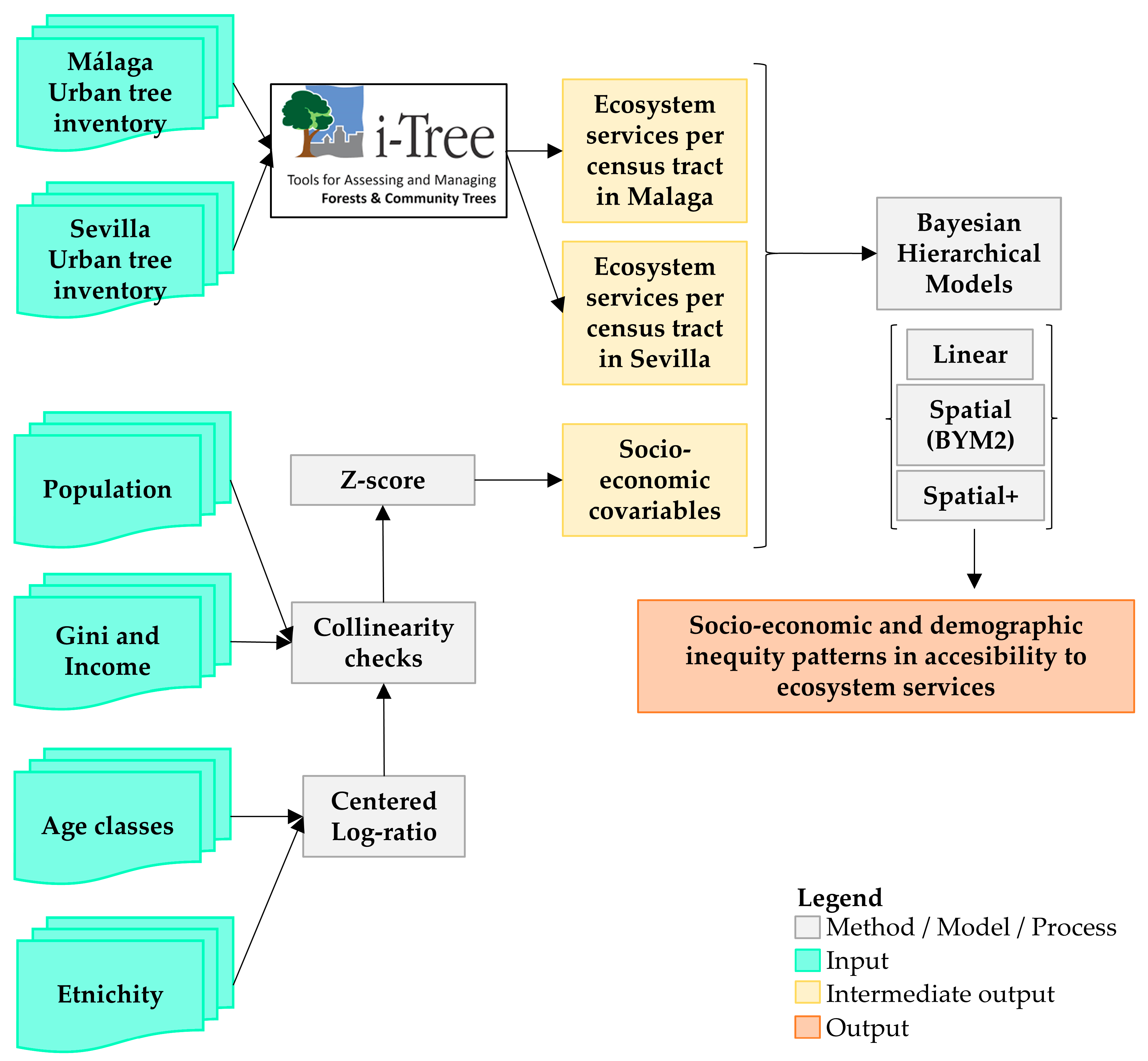
The complete processing and modeling chain is summarized in Figure 1, which may serve as a reference throughout this section.

2.1. Study Area

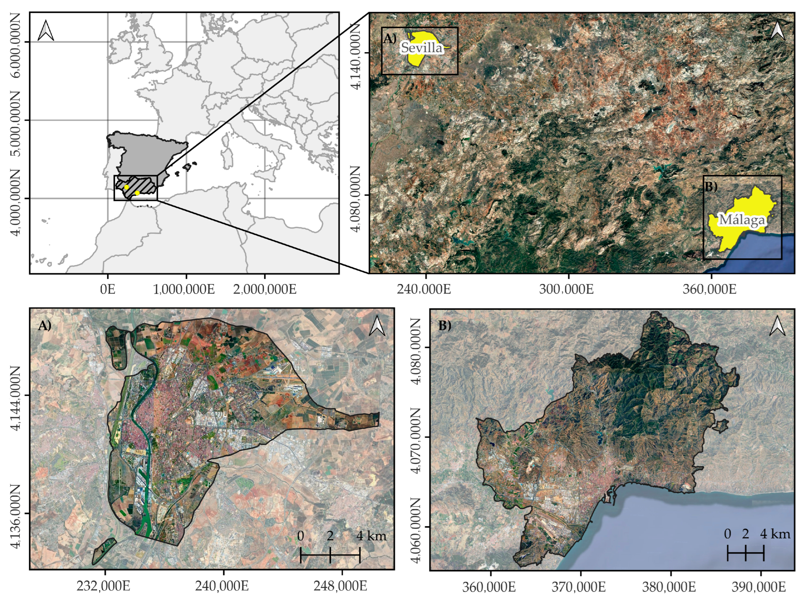
Málaga and Sevilla (Figure 2) are the sixth and fifth most populous cities in Spain, with 599,063 and 689,423 inhabitants, respectively [65]. Both cities have Mediterranean climate conditions (Köppen–Geiger classification Csa) [66]. Located on the coast, Málaga experiences temperate winters and warm summers, averaging 18.5 °C annually with 534 mm of rainfall. Meanwhile, Sevilla records slightly higher yearly averages, registering 19.2 °C and 539 mm of precipitation [67]. Administratively, Málaga comprises 11 municipal districts and 435 census sections, while Sevilla comprises 11 municipal districts and 521 census sections.

2.2. Urban Tree Inventories (UTIs)

A UTI acts as an exhaustive municipal census detailing the location, structural traits, and taxonomy of publicly governed urban trees and palms. Therefore, the dataset inherently bypasses vegetation found in private yards, natural forests, vacant lots, and other unmanaged spaces. The two UTIs differ substantially in their measured structural characteristics and measurement precision. The Sevilla UTI [69] records species, diameter at breast height, total height, and spatial coordinates for each tree, with all variables recorded as continuous numerical values. By contrast, the Málaga UTI (accessed on 6 July 2024; data are not publicly available and accessible only through a visualization portal at https://malaga.mytreerisk.com/) includes additional structural traits: trunk height and crown diameter (measured in both north–south and east–west directions). However, diameter at breast height and height in the Málaga UTI were recorded in discrete diametric and altimetric classes defined by 10 cm and 5 m intervals, respectively.

Although iTree-Eco can produce ES estimates using only DBH and total height, the more comprehensive set of structural variables available in the Málaga dataset is expected to permit more accurate estimation of ES and associated equity patterns. Consequently, differences in data structure and measurement may contribute to variations in model estimates. Although our primary objective is not inter-city comparability of ES estimations, given that these cities serve as independent case studies and comparability is addressed intra-city among different model structures, we harmonized both datasets. Specifically, for Málaga, we retained only height and diameter at breast height values and applied the midpoint value of each altimetric or diametric class to each tree for ES estimation using iTree-Eco.

2.3. iTree-Eco

To quantify the delivery of Ecosystem Services (ES) by the urban forest, we utilized i-Tree Eco v.6.0.40, a standard tool in this field [70,71,72,73]. In the case of Málaga, our analysis of rainfall and pollution levels was restricted to 2015, as this was the latest period offering a comprehensive dataset within the software. Weather variables were sourced directly from the AEMET (State Meteorological Agency) facility situated at Málaga Airport (36°39′58″ N, 4°28′56″ W). Because no air quality monitoring stations in Málaga measured particulate matter less than 2.5 μm, three stations, one outside Malaga administrative area, were selected to capture pollutant concentrations: two stations within the urban matrix (El Atabal: 36°43′46.4″ N, 4°27′56.0″ W; Carranque: 36°43′10.7″ N, 4°26′50.9″ W) and one station in Churriana de la Vega, Granada (37°08′08.3″ N, 3°37′08.9″ W). However, this approach does not introduce substantial bias, as PM_2.5 removal represented only 1.17–2.85% of total particulate matter removal across individual trees. Furthermore, as detailed in subsequent sections, pollutant removal is aggregated for all pollutants. Consequently, PM_2.5 removal by individual trees accounts for an average of 0.44% [min: 0%; max: 0.9%] of total pollutant removal across Malaga’s entire tree population. For Seville, data from 2022 were obtained from the AEMET meteorological station at Seville Airport (37°25′00.5″ N, 5°52′45.3″ W) and the air quality monitoring station at Santa Clara (37°23′54.0″ N, 5°57′05.8″ W), located within the urban matrix.

The i-Tree model provided several key ecosystem service metrics: (1) the yearly mitigation of major air pollutants, specifically SO₂, CO, O₃, NO₂, and particulate matter (both PM₁₀ and PM_2.5); (2) the generation of oxygen; (3) yearly biogenic volatile organic compound (BVOC) emissions, quantified via monoterpene and isoprene equivalents; and (4) the volume of avoided surface runoff annually. These metrics were initially calculated for each specific tree as discrete point data. To model relationships with socioeconomic covariables, we then summarized these individual values at the census tract scale. Further methodological details on i-Tree Eco are available from the i-Tree website (www.itreetools.org, accessed on 5 January 2026) and the program documentation [74].

For the modeling analysis, we considered only microscale ES and disservices, those whose effects are realized in immediate surroundings, as these are most relevant for urban distributional justice analyses. Specifically, we included oxygen production, avoided runoff, BVOC emissions, and total pollutant removal. Transpiration was excluded as a cooling proxy because canopy shading is the predominant mechanism of tree-related temperature reduction [75,76,77]. Additionally, transpiration exhibits high correlation with avoided runoff (r = 0.968) at the individual tree level, rendering inequities in avoided runoff directly applicable to transpiration estimates. Carbon stocks and carbon sequestration were excluded because they were not part of the set of microscale ES and disservices operationalized in our equity model.

2.4. Socio-Economic and Demographic Covariables

To capture the complex socio-demographic landscape, we selected several key covariates to evaluate disparities in ES exposure and access. These included: (1) demographic breakdowns by age cohort and nationality [78]; (2) the Gini coefficient alongside mean household income [79]; and (3) the proportion of residents holding university degrees and unemployment rate [80]. Population data were disaggregated into three components: (1) total population within each census tract, (2) percentage distribution by age group (0–14 years (children), 15–64 years (working-age adults), ≥65 years (elderly)), and (3) percentage distribution by country of origin, hereinafter referred to simply as ethnicity. For the latter, eight origin categories were constructed following the classification scheme of the National Institute of Statistics, which explicitly distinguishes the principal nationalities present in Spain and aggregates the remainder into regional categories: Spain (native-born), Western Europe (France, United Kingdom), Eastern Europe (Romania, Ukraine), other European countries, Morocco, other African countries, Latin America (Cuba, Dominican Republic, Argentina, Bolivia, Colombia, Ecuador, Peru, Venezuela, and other American countries), and Asia-Oceania (China, other Asian countries, and Oceania). These origin categories are broad and heterogeneous, particularly Latin America and Asia-Oceania, which encompass countries with diverse socioeconomic profiles and migration trajectories. Results should be interpreted as average associations for these broad categories, not as country-specific effects.

Ethnicity and age structure variables represent compositional data, as percentages within each census tract sum to 100%, introducing closure constraints that violate standard statistical assumptions and produce spurious correlations between components [81]. To reduce redundancy and improve model parsimony, we merged highly correlated European ethnicity subcategories (Western Europe and other European countries, r = 0.73) into a single category designated as Other Europe, thereby distinguishing this group from Eastern Europe, which is characterized by lower socioeconomic status. This combination conforms to the recommendations for the analysis of compositional data when the components represent analogous information [82,83]. The final ethnicity composition comprised seven categories: Spanish, Eastern Europe, Other Europe, Morocco, Other Africa, Americas, and Asia-Oceania.

To address compositional constraints, we applied centered log-ratio (CLR) transformations to both ethnicity and age composition using compositions R package (v.2.0–8) [84]. The CLR transformation maps compositional data from the simplex to Euclidean space by dividing each component by the geometric mean of all components and taking the natural logarithm. This transformation produces correlated coordinates that preserve the Aitchison geometry of compositional data, eliminates closure constraints, removes spurious correlations induced by the constant-sum constraint, and provides symmetric treatment of all compositional parts [85].

Following CLR transformation, each composition yielded D coordinates subject to a zero-sum constraint. To avoid perfect collinearity with the model intercept, we employed a reference category approach. For ethnicity (seven categories producing seven CLR coordinates), we omitted the CLR coordinate for the Spanish population (the majority group) from models, such that all foreign-born ethnicity effects are interpreted relative to the Spanish baseline. For age structure (three categories producing three CLR coordinates), we omitted the CLR coordinate for the working-age population (15–64 years), thereby interpreting effects for children and elderly populations relative to this reference category. This approach retained D−1 compositional coordinates in the model while preserving interpretability and avoiding singularity issues.

We also included the logarithm of census tract area as a fixed effect to account for size heterogeneity, and to model the elasticity of the area–ES provision relationship empirically. Median building age was included to account for historical landscape legacies, as current canopy could reflect past planting decisions and trees require decades to mature. Older neighborhoods typically support greater canopy cover due to extended establishment periods and cumulative stewardship [86].

Multicollinearity Assessment and Covariate Selection

Before executing the models, we assessed the variables for multicollinearity and correlation. This involved calculating the generalized variance inflation factor (GVIF) via the car package in R (v.3.0–12) [87] alongside Pearson’s correlation coefficients. Whenever predictors exhibited a GVIF above 5 or a Pearson’s |r| > 0.7, we kept only a single variable from that correlated pair [88,89]. Ultimately, both the proportion of university-educated residents and the unemployment rate were dropped from our final analysis, as they demonstrated a GVIF greater than 6 when modeled with the income variable. The rest of the covariates showed acceptable VIFs across both cities (all < 3.5), indicating no multicollinearity issues. Only one correlation pair approached concern thresholds (CLR other European Countries and Log(Income): Málaga r = 0.69, Seville r = 0.63; both < 0.70). Critically, when covariates were residualized in the spatial+ model, by removing their spatial components, no pairwise correlations exceeded 0.60 in either city. The final set of selected variables comprised the Gini index, log-transformed household income, log-transformed total population, CLR-transformed ethnicity, and CLR-transformed age groups, median building age and log-transformed census tract area. To facilitate model fitting in R-INLA, all covariates were standardized (z-score transformation).

2.5. Bayesian Hierarchical Model (BHM)

To deal with spatial structure in the data, we utilized BHMs, which incorporate spatially structured priors into the random effects. Acknowledging these dependencies is vital, failing to do so can result in artificially narrow credibility intervals and biased assessments of coefficient significance [62]. Specifically, we implemented a Latent Gaussian Model (LGM), a BHM variant featuring an additive linear predictor where the data likelihood is conditioned solely on the predictor’s value. These analyses were performed using the Integrated Nested Laplace Approximation (INLA) framework via the R package (v.22.12.16) [90]

Three models (Linear, Spatial, and Spatial+) were fitted independently for each ES (j = 1, …, 4) and for each city. All three models share the common structure defined in Equation (1). The Spatial and Spatial+ models differ in their treatment of covariates: Spatial+ includes residualized covariates, whereas Spatial does not. The Linear model represents the special case where spatially structured effects are not included.

$$Log\left(Y_i\right)\sim Student-t\left({\eta }_i,\varphi ,\nu \right)$$

$${\eta }_i=\alpha +\sum _{k=1}^K{\beta }_{ik}{X}_{ik}+{\theta }_i$$

(1)

$${\theta }_i={\displaystyle \frac{1}{\sqrt{\tau }}}\left(\sqrt{1-\psi }{u}_i+\sqrt{\psi }{v}_i\right)$$

$Y_i$ represents the response for variable j (i.e., ES) in census tract i. It was log-transformed to address its right-skewed distribution. Given evidence of outliers and heavy-tailed residuals in preliminary model exploration, we specified a Student-t likelihood rather than Gaussian likelihood. The Student-t likelihood provides robustness by down-weighting extreme observations, thereby limiting their influence on fixed-effect estimates and spatial random effects. In non-spatial models, replacing the Gaussian with a Student-t likelihood substantially improved model fit. In contrast, Gaussian-likelihood models with spatial random effects exhibited numerical instability and signs of overfitting, indicating that a Gaussian specification was inadequate for these data. $\varphi$ denotes the precision of the Student-t. The degrees-of-freedom parameter ($\nu$) was estimated from the data to allow the tail behavior to adapt to the empirical distribution.

${\eta }_i$ is the linear predictor. $\alpha$ represents the model intercept. ${\beta }_k$ represents the fixed effect for the covariate k on ES j. ${\theta }_i$ represents the effect from a BYM2 model. BYM2 is an extension of the BYM model (Besag-York-Mollié Model) [91], proposed by Riebler et al. [92], where a scaled variance approximately equal to one exists between the i.i.d. (independent and identically distributed) effects and the CAR (Conditional Autoregressive Model) components of the BYM2. The main advantage of the BYM2 model is its ability to separately capture the impact of spatial dependence and the effect of data variability. The random effects $v_i$, which constitute a structured effect via the CAR prior, and $u_i$, modeled as an i.i.d. effect, together form the implementation of BYM2. These effects are modeled through $\tau$, which represents the marginal precision contribution from both random effects, and $\psi$, which indicates the fraction of the variance explained by the spatially structured random effect.

Both parameters were specified using penalized complexity (PC) priors [93], assuming $P\left(1/\sqrt{\tau }>2\right)=0.5$, and $P\left(\psi >0.5\right)=0.5$. In contrast to the precision parameter $\tau$, the resulting PC prior for $\psi$ cannot be specified in closed form due to the dependence on the graph structure of the Gaussian Markov Random Field [92]. For fixed effects, a weakly informative normal prior with standard deviation of 1000 was specified. The likelihood precision, $\varphi$, followed the default Gamma(shape = 1, rate = 5 × 10⁻⁵) prior. The degrees-of-freedom parameter (ν) was assigned its default prior specification in R-INLA, a log-Gamma(1, 0.00005), which places weak regularization on tail behavior while allowing the likelihood to be informed primarily by the data.

2.5.1. Spatial+ Implementation

Spatial+, proposed by Dupont et al. [64], mitigates spatial confounding by explicitly separating the spatial structure of the covariates from their local variation prior to effect estimation. It shows good properties for alleviating spatial confounding when traditional spatial models can lead to biased effect estimates when the cause is that covariates are collinear with spatial random effects. To address this, the Spatial+ approach removes spatial structure from covariates prior to model fitting while preserving non-spatial variation. In the first step, a spatial model is fitted to each covariate to filter out its spatial dependence, yielding spatially uncorrelated residuals (${\mathrm{R}}_{i,k}$) (Equation (2)). Residuals from this model represent the covariate with purely spatial structure removed, thereby isolating the non-spatial component

$${\mathrm{X}}_{i,k}\sim \mathrm{N}\left({\mathsf{\eta }}_{i,k},{\mathsf{\varphi }}_k\right)$$

$${\mathsf{\eta }}_{i,k}=\alpha +{\mathrm{w}}_{i,k}$$

(2)

$${\mathrm{R}}_{i,k}={\mathrm{X}}_{i,k}-{\mathsf{\eta }}_{i,k}$$

Covariate $X_k$ was regressed against spatial effects using an intrinsic conditional autoregressive (ICAR) model, also known as the Besag model $\left\{{\mathrm{w}}_{i,k}\right\}$. A PC prior was implemented in the standard deviation of the ICAR model assuming a 0.5 probability for it to exceed 1. We used the ICAR model rather than BYM2 for covariate residualization because the latter includes an unstructured heterogeneity component representing non-spatial random variation that should be preserved in the covariates to ensure valid inference. The residualization of the covariates was preceded by an assessment of the presence of spatial autocorrelation in all covariates using Global Moran’s I statistic under randomization using spdep R package v.1.4-1 [94,95,96]. For Málaga, spatial autocorrelation tests revealed significant positive spatial structure across all covariates (all p < 2.2 × 10⁻¹⁶), with Moran’s I values ranging from 0.204 to 0.684 (z-scores: 7.19 to 23.94). The strongest spatial pattern was observed in logarithm of the income (I = 0.684, z = 23.94), followed by logarithm of the census tract area (I = 0.645, z = 22.62), while logarithm of census tract population exhibited the weakest spatial structure (I = 0.204, z = 7.19). For Sevilla, all covariates similarly demonstrated highly significant spatial autocorrelation (all p < 2.2 × 10⁻¹⁶), with Moran’s I ranging from 0.166 to 0.747 (z-scores: 6.51 to 29.01). The most pronounced spatial pattern was found in logarithm of the income (I = 0.747, z = 29.01), while logarithm of census tract population showed the lowest spatial structure (I = 0.166, z = 6.51). Given that all covariates demonstrated statistically significant spatial autocorrelation, we concluded that all covariates required residualization using the Spatial+ approach to mitigate spatial confounding bias in covariate effect estimates [64].

In the second step, these covariate residuals are substituted for the original covariates in the response model (Equation (1)). Crucially, the response variable remains in its original scale, and this final regression includes its own spatial random effect (BYM2). Regressing covariates against spatial residuals isolates their local variation, allowing the spatial term in the second stage to absorb confounding patterns without competing with predictors. This yields approximately unbiased covariate effects when covariates exhibit sufficient local variation. Remaining bias depends on how well the covariate’s local signal can be distinguished from the confounding field.

2.5.2. Model Diagnostics and Performance Evaluation

Model performance was rigorously assessed using multiple Bayesian diagnostic metrics implemented in INLA. The marginal likelihood (mlik) was calculated to quantify overall model evidence in a Bayesian framework, enabling formal model comparison across the three competing specifications [90]. Higher marginal likelihood values indicate greater support from the observed data. The Watanabe-Akaike information criterion (WAIC) [97] was computed to assess out-of-sample predictive accuracy while accounting for model complexity, with lower values indicating superior predictive performance. WAIC is asymptotically equivalent to leave-one-out cross-validation and provides a more stable alternative to information criteria based on point estimates [98,99]. Bayesian R² [100] was derived from 10,000 posterior predictive samples to quantify the proportion of variance in log-transformed scale explained by the fitted model. Leave-one-out cross-validation was operationalized via Conditional Predictive Ordinates (CPO), which estimate prediction accuracy when each observation is excluded from model fitting [101]. We computed Log Score from CPO (LSCP) $(LSCP=-{\sum }_{i=1}^n\mathrm{l}\mathrm{o}\mathrm{g}({\mathrm{CPO}}_i))$ as a summary statistic for model comparison, with lower values indicating superior predictive performance. Finally, posterior predictive calibration was evaluated using the Probability Integral Transform (PIT), where PIT values should follow a uniform distribution if the model produces appropriately calibrated predictions that properly quantify prediction uncertainty [102,103]. The Kolmogorov–Smirnov test was applied to assess whether observed PIT values deviate significantly from uniformity (p > 0.05 indicates well-calibrated predictions).

Posterior predictive checks were systematically conducted to validate models’ fit and assumptions across multiple dimensions. Eight diagnostic plots was generated to assess: (1) point-wise agreement between observed and fitted values to evaluate overall model accuracy; (2) patterns in residuals versus fitted values to detect heteroscedasticity or systematic deviations from linearity; (3) quantile-quantile plots of standardized residuals; (4) PIT histograms to evaluate whether posterior predictive distributions were properly calibrated for the observed data; (5) empirical cumulative distribution functions comparing observed data against posterior predictive samples, quantifying whether the fitted model generates realistic data distributions that match the observed marginal distribution; (6) overlaid density plots of posterior predictive samples and observed data to visually assess distributional agreement and detect systematic departures in tails or central tendency; (7) sorted CPO on a logarithmic scale to identify observations with poor leave-one-out predictive performance; and (8) Moran scatterplots of residuals against spatially lagged residuals with Moran’s I significance testing.

3. Results

3.1. Urban Forest Structure and Composition

The analysis revealed distinct differences in the abundance and density of the urban forest between the two cities (

Table 1. Urban forest structure for Malaga and Sevilla.

Metric	Malaga	Sevilla
Total trees	104,107	183,485
Mean density (trees/km2)	2172	3436
Min density (trees/km2)	0.55	8.77
Max density (trees/km2)	10,150	10,782

). Sevilla supported a substantially larger total tree population, 76% greater than Málaga, alongside a higher mean density. Málaga, while lower in both total trees and mean density, exhibited a noticeably wider variance in distribution, suggesting a more uneven spatial arrangement of trees across the city. Despite its smaller tree population, Málaga demonstrates higher taxonomic diversity with 304 species from 180 genera and 61 families, compared to Sevilla’s 273 species from 160 genera and 64 families, indicating a more diverse species composition in Málaga’s urban forest.

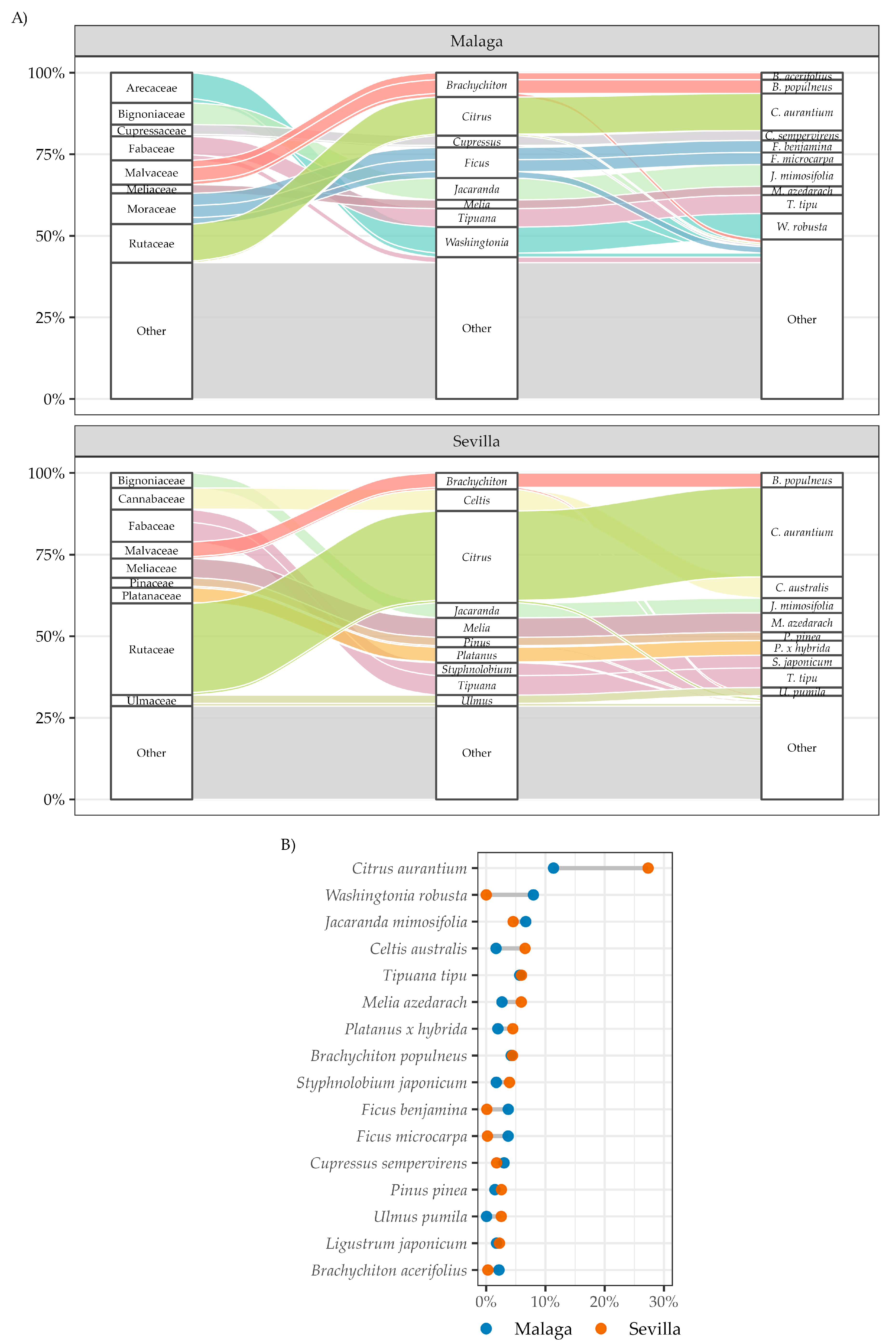
Regarding species dominance (Figure 3), Citrus aurantium dominates both urban forests, but it represents a 27% (n = 50,134) of Sevilla’s inventory versus only 11% (n = 11,822) in Málaga. The top ten species in Málaga collectively account for 52% of all trees, with relatively balanced representation led by C. aurantium, Washingtonia robusta (8%, n = 8286), and Jacaranda mimosifolia (7%, n = 6942). In contrast, Sevilla’s top ten species show greater concentration, with C. aurantium alone comprising over a quarter of the urban forest, followed by Celtis australis (7%, n = 12,021) and Tipuana tipu (6%, n = 10,916). Both cities share five species among their most abundant taxa, though in different proportions: C. aurantium (Málaga: 11%, n = 11,822; Sevilla: 27%, n = 50,134), T. tipu (Málaga: 6%, n = 5892; Sevilla: 6%, n = 10,916), J. mimosifolia (Málaga: 7%, n = 6942; Sevilla: 5%, n = 8342), Melia azedarach (Málaga: 3%, n = 2775; Sevilla: 6%, n = 10,852), and Brachychiton populneus (Málaga: 4%, n = 4393; Sevilla: 4%, n = 8134).

Analysis of the most abundant genera and families further highlighted compositional distinctness. Both cities shared five dominant genera: Citrus (Málaga: 12%, n = 12,343; Sevilla: 28%, n = 51,537), Tipuana (Málaga: 6%, n = 5892; Sevilla: 6%, n = 10,916), Brachychiton (Málaga: 7%, n = 7758; Sevilla: 5%, n = 9226), Jacaranda (Málaga: 7%, n = 6943; Sevilla: 5%, n = 8453), and Ligustrum (Málaga: 3%, n = 3033; Sevilla: 4%, n = 7413). Málaga’s composition was characterized by Ficus (9%, n = 9786) and Washingtonia (9%, n = 9619), neither of which appeared in Sevilla’s top ten genera, where Celtis (7%, n = 12,198) and Melia (6%, n = 10,852) were prominent instead. At the family level, Málaga is dominated by Arecaceae (15%, n = 15,112), reflecting high palm abundance, followed by Fabaceae (14%, n = 14,210) and Rutaceae (12%, n = 12,345). In the case of Seville, composition was heavily marked by Rutaceae (28%, n = 51,542) and Fabaceae (16%, n = 29,631), with a notable presence of Oleaceae (8%, n = 13,930), whereas Arecaceae did not rank among its top ten families.

3.2. Urban Forest Ecosystem Services Provision

Sevilla consistently outperformed Malaga in gross and normalized provision of avoided runoff, oxygen production, and pollutant removal (

Table 2. Gross, per unit area, and per tree annual ecosystem service (ES) provision of the urban forests of Málaga and Sevilla. For normalized provisions, values in parentheses represent the observed minimum and maximum.

Ecosystem Service	Malaga	Sevilla
Gross provision
Avoided runoff (hm3/year)	0.011	0.048
Oxygen production (Tn/year)	3.26	6.99
Pollutant removal (Tn/year)	37.6	92.7
BVOC emissions (Tn/year)	15.1	14.5
Provision per unit area
Avoided runoff (L/m2/year)	0.24 (0.0002–1.47)	0.79 (0.002–3.82)
Oxygen production (kg/m2/year)	0.07 (0.00003–0.31)	0.13 (0.0003–0.49)
Pollutant removal (g/m2/year)	0.84 (0.0006–5.15)	1.52 (0.004–7.39)
BVOC emissions (g/m2/year)	0.28 (0–3.77)	0.23 (0–1.68)
Provision per tree
Avoided runoff (L/tree/year)	103.3 (0–3798)	261.4 (1.0–15,896)
Oxygen production (kg/tree/year)	31.5 (0.1–273.5)	38.2 (0.3–508)
Pollutant removal (g/tree/year)	361.3 (0–13,281.3)	505.5 (1.9–30,735.6)
BVOC emissions (g/tree/year)	144.8 (0–25,576)	80.6 (0–999.8)

). The per-tree values further suggest that Sevilla’s trees are, on average, larger or more productive. The one notable exception was BVOC emissions: despite having fewer trees, Málaga’s urban forest produced higher total emissions (15.1 vs. 14.5 Tn/year), with a per-tree mean nearly double that of Sevilla (144.8 vs. 80.6 g/tree/year), pointing to a species composition more prone to BVOC release.

3.3. Bayesian Hierarchical Model Results

3.3.1. Models’ Performance, Hyperparameters and Variance Partitioning

Model performance evaluation revealed consistent patterns across all ES within each city, with spatial models demonstrating substantial improvements over Linear model (

Table 3. Model fit and predictive performance. WAIC refers to Watanabe Akaike Information Criterion; Mlik refers to Model likelihood; Bayesian R² is reported with the posterior mean and 95% credibility interval; LSCP refers to log score calculated based on Conditional Predictive Ordinates.

	Avoided Runoff		BVOCs Production		Oxygen Production		Removed Pollutants
Variable	Malaga	Sevilla	Malaga	Sevilla	Malaga	Sevilla	Malaga	Sevilla
WAIC
Linear	1362.1	1423.1	1554.6	1639.5	1239.0	1290.6	1363.2	1423.1
Spatial	1224.3	1166.0	1460.2	1417.5	1123.8	990.7	1226.1	1168.2
Spatial+	1202.7	1165.5	1436.7	1405.3	1105.1	991.7	1202.9	1165.3
Mlik
Linear	−762.6	−796.7	−859.5	−900.8	−701.9	−731.1	−763.2	−796.7
Spatial	−510.1	−428.1	−614.1	−538.2	−452.6	−349.0	−510.6	−426.0
Spatial+	−534.5	−440.1	−644.8	−550.0	−478.0	−360.8	−535.1	−440.3
Bayesian R2
Linear	40.2	44.4	34.1	41.4	45.0	46.9	39.9	44.4
	[31.9, 47.5]	[36.6, 51.0]	[22.0, 43.5]	[35.2, 47.3]	[37.3, 51.6]	[39.9, 52.9]	[31.4, 47.3]	[36.6, 51.0]
Spatial	56.7	69.7	44.0	65.9	60.6	72.4	56.4	69.6
	[46.8, 66.5]	[62.8, 75.9]	[30.9, 55.9]	[58.8, 72.7]	[51.7, 69.5]	[66.0, 78.1]	[46.5, 66.4]	[62.3, 76.5]
Spatial+	61.4	71.9	48.7	67.6	66.3	73.8	61.3	71.8
	[51.8, 70.2]	[65.1, 78.0]	[37.1, 59.2]	[60.0, 74.7]	[57.2, 74.7]	[67.1, 80.1]	[51.6, 70.0]	[65.0, 78.0]
LSCP
Linear	681.1	711.6	777.3	819.8	619.6	645.3	681.6	711.6
Spatial	612.9	584.7	730.5	711.2	562.8	497.9	613.0	586.1
Spatial+	603.1	585.8	718.4	706.8	555.4	499.8	603.1	585.8

). Detailed model diagnostics are provided in the Supplementary Material. Model predictions, uncertainty estimates, and residual patterns are presented in Figures S1–S8 (Linear model), Figures S9–S16 (Spatial model), and Figures S17–S24 (Spatial+ model). Posterior predictive checks are similarly organized in Figures S25–S48, following the same city and model structure.

Accounting for spatial autocorrelation significantly improved model fit, with both Spatial and Spatial+ models consistently outperforming the Linear model across all performance metrics. In Málaga, the Spatial+ model demonstrated superiority over the Spatial model across all four ES. WAIC values decreased by 6.1–11.7% in spatial models relative to the Linear model. The greatest improvements were observed for avoided runoff (11.7% reduction) and removed pollutants (11.8% reduction), while BVOC production showed the smallest improvement (7.6%). Model likelihood improved by 33.1% for BVOC production to 46.3% for oxygen production in spatial models, with a marginal performance decline of 4.6–5.4% for Spatial+ relative to the Spatial model. LSCP values improved by 6.1–11.8% in spatial models, with marginal additional improvements of 1.2–1.6% for Spatial+ models over Spatial models. Bayesian R² values showed posterior means rising from 34.1 to 45.0% in the Linear model to 44.0–66.3% in the Spatial+ model ES. The largest gains in explained variance were observed for avoided runoff (Linear: 40.2% [31.9, 47.5]; Spatial+: 61.4% [51.8, 70.2]) and oxygen production (Linear: 45.0% [37.3, 51.6]; Spatial+: 66.3% [57.2, 74.7]). BVOC production exhibited the lowest explained variance across all models, although the Spatial+ model still achieved a posterior mean of Bayesian R², representing a 29.9% relative increase over the Linear model versus a 22.5% relative to a spatial model.

Spatial model incorporation in Sevilla demonstrated more pronounced performance improvements compared to Málaga. WAIC reductions ranged from 13.5% to 23.2% relative to the Linear model. Model likelihood values exhibited parallel patterns, with improvements ranging from 44.5% for BVOC production to 61.4% for avoided runoff in the Spatial model. LSCP values decreased by 13.5–23.2% in spatial models. Bayesian R² values in Sevilla were consistently higher than in Málaga across all models and ES. The Linear model explained 41.4–46.9% of variance, while the Spatial+ model achieved 67.6–73.8%. Consistent with Málaga, BVOC production showed the lowest R² values across all models.

Consistently across both cities, the inclusion of spatially structured effects reduced the percentage of variance explained by the observation-level likelihood while correspondingly decreasing hyperparameter magnitudes (

Table 4. Mean and 95% credibility intervals of the hyperparameters’ posterior distributions. $1/\sqrt{\varphi }$ refers to the standard deviation of the Student-t likelihood; $\nu$ refers to the degrees-of-freedom of the Student-t likelihood; $1/\sqrt{\tau }$ refers to the marginal spatial standard deviation of the BYM2 effect; and, $\psi$ refers to the contribution of the spatial component of the BYM2 effect (Conditional Autoregressive Model, CAR) versus the i.i.d. component.

	Avoided Runoff		BVOCs Production		Oxygen Production		Removed Pollutants
Hyper.	Malaga	Sevilla	Malaga	Sevilla	Malaga	Sevilla	Malaga	Sevilla
$1/\sqrt{\varphi }$
Linear	1.22	0.99	1.73	1.17	1.04	0.85	1.23	0.99
	[1.08, 1.38]	[0.89, 1.11]	[1.42, 2.13]	[1.08, 1.27]	[0.93, 1.16]	[0.77, 0.94]	[1.08, 1.39]	[0.89, 1.11]
Spatial	0.99	0.71	1.54	0.87	0.85	0.59	1.00	0.70
	[0.84, 1.17]	[0.62, 0.80]	[1.21, 1.99]	[0.76, 0.98]	[0.73, 0.99]	[0.52, 0.67]	[0.84, 1.18]	[0.61, 0.80]
Spatial+	0.93	0.67	1.40	0.84	0.79	0.57	0.93	0.67
	[0.80, 1.07]	[0.59, 0.76]	[1.16, 1.70]	[0.74, 0.95]	[0.68, 0.91]	[0.50, 0.65]	[0.80, 1.07]	[0.59, 0.76]
$\nu$
Linear	4.16	4.40	2.96	6.73	4.79	5.15	4.11	4.40
	[3.08, 5.80]	[3.18, 6.28]	[2.42, 3.77]	[4.31, 10.74]	[3.42, 6.88]	[3.63, 7.52]	[3.05, 5.71]	[3.18, 6.28]
Spatial	3.87	4.92	2.81	6.16	4.54	5.01	3.83	5.08
	[2.86, 5.48]	[3.46, 7.29]	[2.32, 3.59]	[4.00, 10.05]	[3.23, 6.64]	[3.54, 7.32]	[2.85, 5.39]	[3.48, 7.71]
Spatial+	4.61	6.33	3.07	7.27	6.13	6.41	4.53	6.35
	[3.29, 6.63]	[4.17, 9.88]	[2.52, 3.85]	[4.01, 13.73]	[3.98, 9.73]	[3.78, 11.53]	[3.28, 6.42]	[4.12, 10.07]
$1/\sqrt{\tau }$
Linear	-	-	-	-	-	-	-	-
Spatial	0.60	0.52	0.60	0.67	0.53	0.47	0.60	0.53
	[0.47, 0.75]	[0.44, 0.62]	[0.45, 0.76]	[0.56, 0.79]	[0.40, 0.68]	[0.40, 0.55]	[0.47, 0.76]	[0.44, 0.63]
Spatial+	0.78	0.60	0.84	0.74	0.73	0.52	0.78	0.60
	[0.66, 0.91]	[0.51, 0.70]	[0.72, 0.98]	[0.62, 0.88]	[0.60, 0.87]	[0.43, 0.62]	[0.65, 0.91]	[0.51, 0.70]
$\psi$
Linear	-	-	-	-	-	-	-	-
Spatial	0.96	1.00	0.94	0.97	0.94	0.98	0.95	0.97
	[0.82, 1.00]	[1.00, 1.00]	[0.75, 1.00]	[0.88, 1.00]	[0.78, 1.00]	[0.89, 1.00]	[0.76, 1.00]	[0.91, 1.00]
Spatial+	0.98	0.98	0.98	0.97	0.97	0.98	0.98	0.98
	[0.91, 1.00]	[0.94, 1.00]	[0.89, 1.00]	[0.89, 1.00]	[0.88, 1.00]	[0.90, 1.00]	[0.92, 1.00]	[0.94, 0.99]

and

Table 5. Mean and 95% credibility intervals of the percentage of variance explained by each model component. Obs. Level refers to the observation-level variance contribution; Fixed refers to fixed effects contribution; Spatial effect refers to BYM2 spatial component contribution; Cov[F, S] refers to the percentage explained by twice the covariance between fixed and BYM2 effects.

	Avoided Runoff		BVOCs Production		Oxygen Production		Removed Pollutants
Variable	Malaga	Sevilla	Malaga	Sevilla	Malaga	Sevilla	Malaga	Sevilla
Obs. Level
Linear	59.8	55.6	65.9	58.6	55.0	53.1	60.0	55.7
	[52.4, 68.1]	[49.0, 63.5]	[56.4, 77.9]	[52.6, 64.8]	[48.4, 62.6]	[47.1, 59.8]	[52.6, 68.3]	[49.1, 63.3]
Spatial	43.1	30.4	55.7	34.1	39.4	27.7	43.4	30.3
	[33.4, 52.9]	[23.7, 37.6]	[44.1, 68.6]	[27.2, 41.2]	[30.5, 48.2]	[21.8, 34.1]	[33.5, 53.3]	[23.9, 37.0]
Spatial+	38.6	28.1	51.4	32.4	33.9	26.2	38.7	28.2
	[29.9, 48.2]	[22.1, 35.0]	[40.9, 62.9]	[25.3, 40.0]	[25.3, 42.8]	[20.0, 33.0]	[30.0, 48.3]	[22.1, 34.9]
Fixed
Linear	40.2	44.4	34.1	41.4	45.0	46.9	40.0	44.3
	[31.9, 47.6]	[36.5, 51.0]	[22.1, 43.6]	[35.2, 47.4]	[37.4, 51.6]	[40.2, 52.9]	[31.7, 47.4]	[36.7, 50.9]
Spatial	44.1	47.1	35.2	40.9	50.6	48.0	43.9	47.1
	[34.1, 54.9]	[40.3, 54.3]	[24.4, 46.6]	[33.7, 48.6]	[40.3, 61.7]	[41.6, 54.6]	[33.6, 55.0]	[40.3, 54.2]
Spatial+	18.7	35.4	14.7	29.8	22.1	38.5	18.6	35.4
	[14.0, 23.6]	[30.3, 40.5]	[10.2, 19.6]	[24.8, 35.1]	[17.2, 27.4]	[33.4, 43.8]	[14.0, 23.6]	[30.3, 40.5]
Spatial effect
Linear	-	-	-	-	-	-	-	-
Spatial	15.9	23.7	9.0	25.1	14.5	24.8	15.8	23.8
	[9.6, 23.5]	[17.4, 30.5]	[4.5, 14.9]	[18.3, 32.1]	[8.5, 21.8]	[18.9, 31.1]	[9.5, 23.3]	[18.0, 30.2]
Spatial+	38.4	33.4	30.2	35.9	39.2	33.1	38.3	33.4
	[29.8, 47.0]	[26.7, 40.0]	[21.7, 38.8]	[28.4, 43.4]	[30.4, 48.1]	[26.4, 40.4]	[29.8, 46.8]	[26.8, 40.1]
Cov[F,S]
Linear	-	-	-	-	-	-	-	-
Spatial	−3.1	−1.2	0.0	−0.1	−4.5	−0.6	−3.0	−1.2
	[−12.4, 4.6]	[−7.5, 4.2]	[−6.4, 5.7]	[−6.4, 5.3]	[−14.3, 3.7]	[−6.1, 4.3]	[−12.2, 4.7]	[−7.5, 4.2]
Spatial+	4.3	3.0	3.7	1.9	4.8	2.1	4.3	3.0
	[1.6, 6.9]	[−0.4, 6.1]	[1.6, 5.8]	[−1.5, 4.9]	[1.8, 7.7]	[−1.4, 5.3]	[1.6, 6.9]	[−0.3, 6.1]

). In the Linear model, observation-level likelihood accounted for an average variance explained of 60.18% in Málaga and 55.75% in Sevilla. Following the incorporation of spatial effects, this variance component decreased by 15.4% (BVOCs) to 28.3% (oxygen production) in Málaga, and by 41% (BVOCs) to 47.8% (oxygen production) in Sevilla. The degrees of freedom for Student’s t-distribution decreased on average in Málaga but increased in Sevilla. In the Spatial+ model, this hyperparameter increased by an average of 13.18% in Málaga and 30.16% in Sevilla, suggesting that this model fits distributions requiring lighter tails.

Fixed effects explained similar variance percentages between Linear and Spatial models, ranging from 34.10% (BVOCs) to 45% (oxygen production) in Málaga’s Linear model, 41.4% (BVOCs) to 46.9% (oxygen production) in Sevilla’s Linear model, and 35.2% to 50.6% in Málaga’s Spatial model versus 40.9% to 48% in Sevilla’s Spatial model for the same ES. These average increases of 8.78% (Málaga) and 3.38% (Sevilla) in fixed effects variance upon including the BYM2 effect contrast sharply with the Spatial+ model, where fixed effects variance decreased by 53.6% in Málaga and 21.6% in Sevilla relative to the Linear model. Consequently, in the Spatial+ model, fixed effects explained 14.70% (BVOCs) to 22.10% (oxygen production) in Málaga and 29.8% to 38.5% (same ES) in Sevilla.

The BYM2 contribution to explained variance was nearly double in Sevilla (mean: 24.35%, range: 23.70–25.10%) compared to Málaga (mean: 13.80%, range: 9–15.90%). For the Spatial+ model, contributions were more comparable between Málaga (mean: 36.5%, range: 30.2–38.4%) and Sevilla (mean: 33.9%, range: 33.10–35.9%). Notably, the entire BYM2 contribution to explained variance derived from the CAR component rather than the iid component, with the hyperparameter ψ consistently exceeding 0.95 across both cities and models. Finally, covariance between fixed effects and spatial effects explained minimal variance, averaging higher in Málaga than Sevilla, with negative values for the Spatial model (−2.65% and −0.775%, respectively) and positive values for the Spatial+ model (4.275% and 2.5%, respectively).

3.3.2. Inequity Patterns in Accessibility to Ecosystem Services

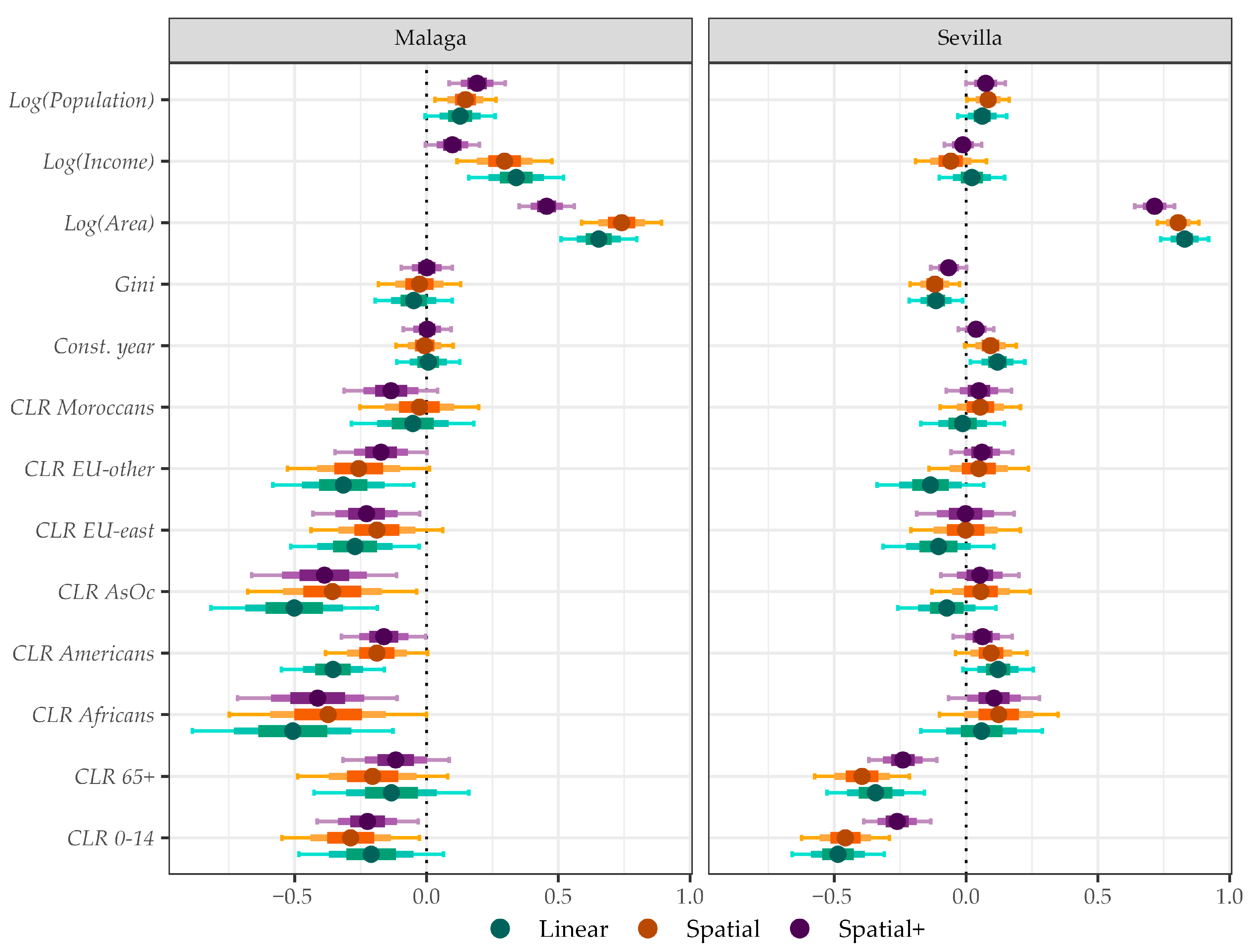
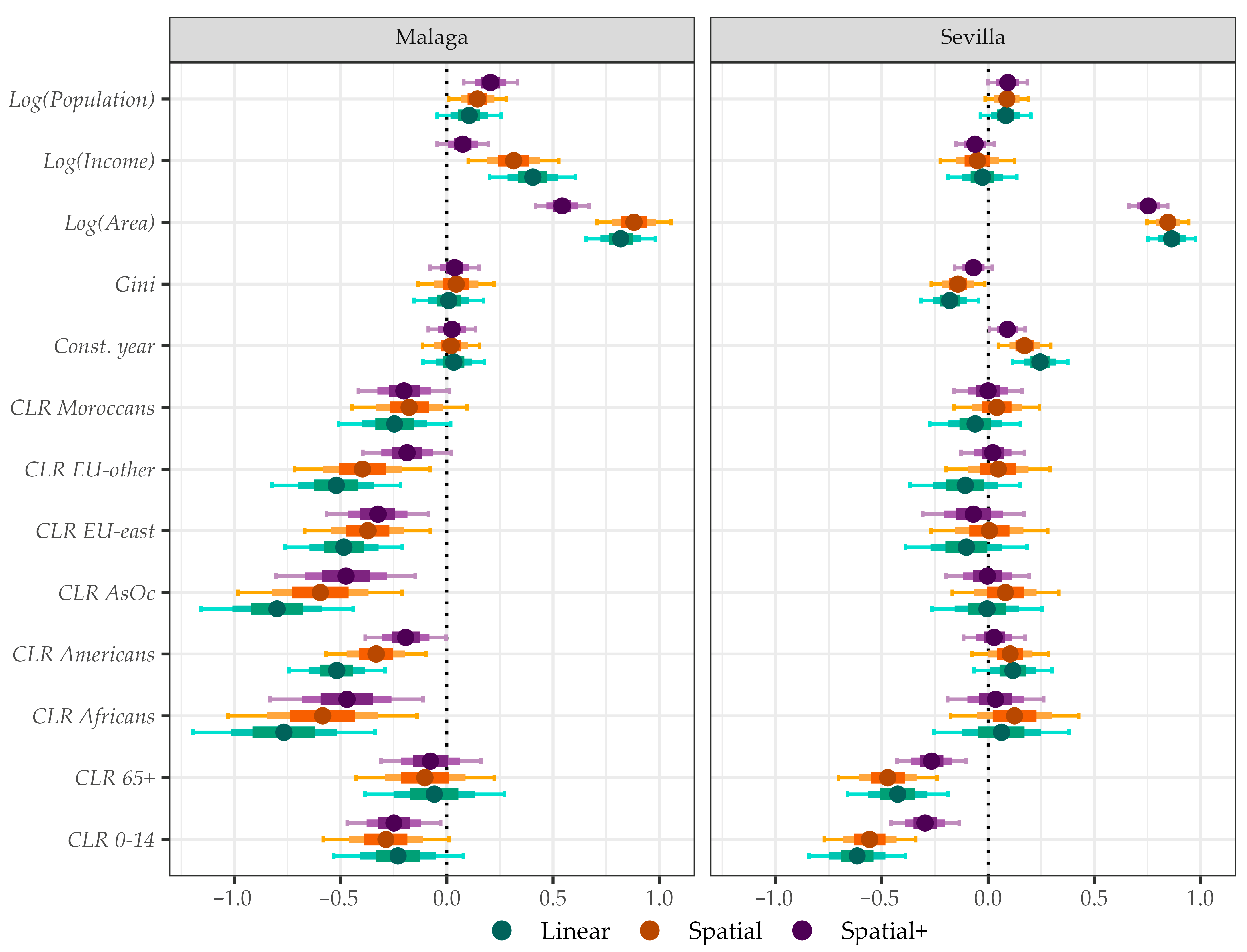
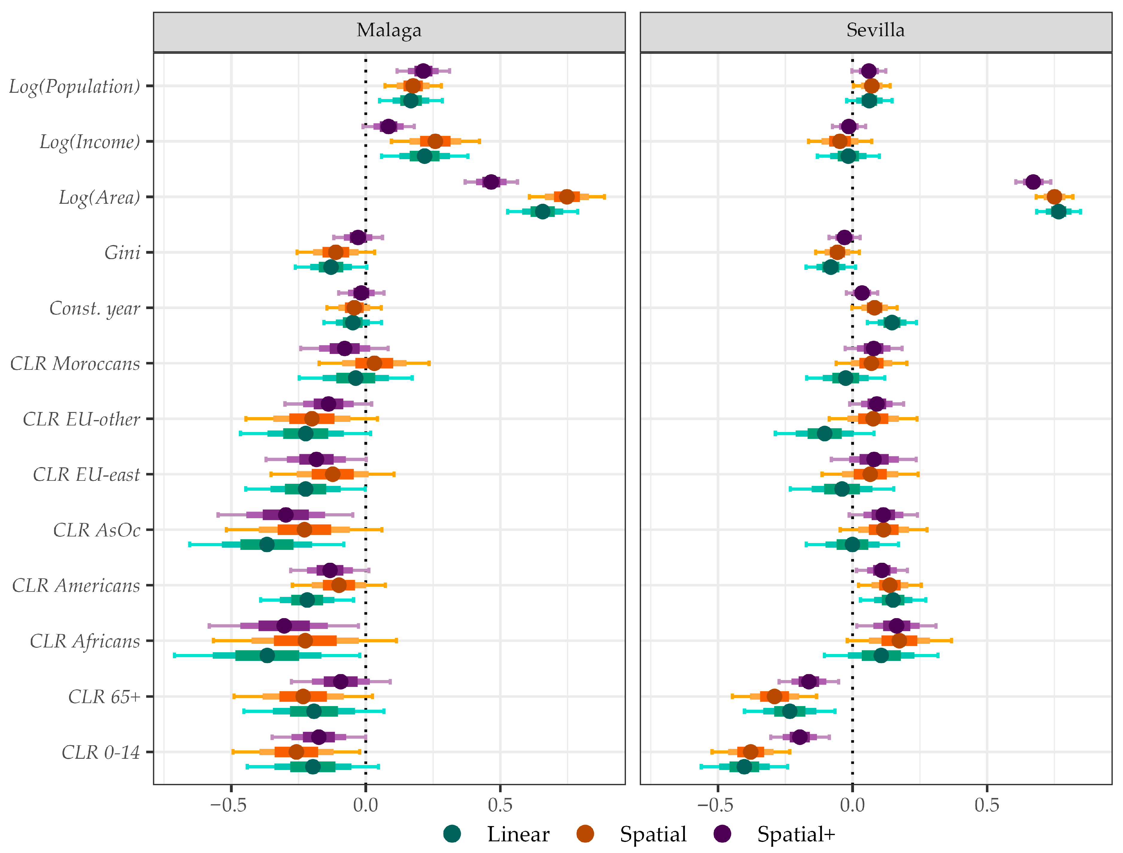
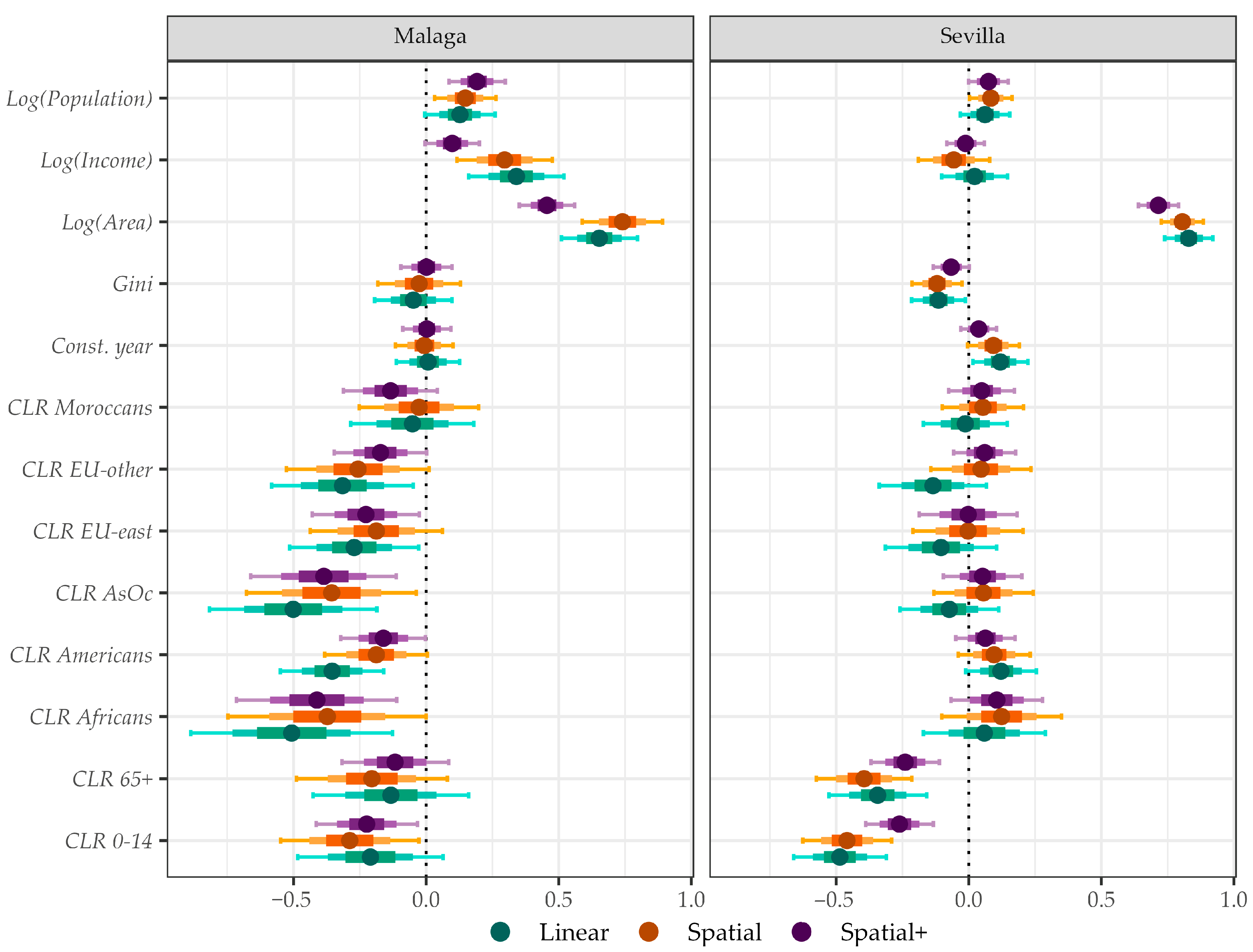
Fixed-effect estimates, i.e., socio-economic and demographic inequity patterns, revealed differences among Linear, Spatial, and Spatial+ model specifications, with patterns varying substantially across cities and, to a lesser extent, across ES (Figure 4, Figure 5, Figure 6 and Figure 7; Table S1). The most pronounced between-model discrepancies occurred for Area and Income covariates, where Spatial+ consistently altered both effect magnitudes and credibility. Conversely, age and ethnicity exhibited greater stability across model specifications.

In Málaga, income effects demonstrated strong positive associations with all ES under Linear and Spatial specifications (means: 1.03–1.41% per 1% increase in income), with 95% credible intervals excluding zero. Spatial+ amplified these effects approximately threefold, but substantially wider credible intervals marginally included zero, rendering the effect non-credible at the 95% probability. Although Spatial+ provided insufficient evidence to conclusively establish a positive relationship between income and ES provision, moderate directional evidence (probability of direction, PD = 0.89–0.97) suggested a likely positive association. In contrast, Sevilla showed non-credible income effects across all three models.

Gini inequality produced divergent results between cities. In Málaga, all three models estimated non-credible effects. Weak evidence suggested a potential negative relationship between Gini and total oxygen production, with Linear and Spatial models indicating 0.97 and 0.93 PD of a negative effect, respectively, though this evidence remained insufficient for conclusive inference. In Sevilla, Linear and Spatial models estimated credible negative effects of Gini on ES provision, whereas Spatial+ detected no credible relationships with any ES, with removed pollutants showing the strongest evidence (PD = 0.97). Under Linear and Spatial specifications, each 1% increase in the Gini index within a census tract was associated with reductions of −3.31% [−6.18%, −0.40%] or −3.45% [−6.10%, −0.75%] in avoided runoff, −5.18% [−8.92%, −1.35%] or −4.11% [−7.62%, −0.50%] in BVOCs production, −2.36% [−4.98%, 0.32%] or −1.64% [−3.98%, 0.73%] in oxygen production, and −3.31% [−6.18%, −0.40%] or −3.47% [−6.13%, −0.75%] in removed pollutants, with the first value corresponding to Linear and the second to Spatial estimates for each service.

Total population in census tracts exhibited progressive strengthening of effects from Linear to Spatial to Spatial+ models in Málaga, but remained stable across specifications in Sevilla. In Málaga, Linear models produced non-credible effects, with the sole exception of oxygen production. Spatial and Spatial+ models consistently identified positive relationships between population size and ES provision across all services; each 1% increase in census tract population is related to an average increase in provision ranging from 0.44% to 0.54% under the Spatial model and from 0.77% to 0.86% under Spatial+, with variation attributable to ES type. In Sevilla, only the Spatial model estimated relationships that achieved 95% credibility, albeit with effects marginally distinct from zero. Notably, in Sevilla, census tracts with larger populations were not estimated to be associated with greater BVOC production by urban trees under any model specification.

Compositional age classes showed consistent negative effects across models and cities, suggesting that census tracts with higher proportions of vulnerable age groups, young residents and/or elderly populations, were associated with reduced ES provision by urban trees. CLR 0–14 years (proportion of young residents) demonstrated strong negative associations with all ES in both cities. In Málaga, Spatial and Spatial+ models consistently estimated credible negative relationships across all ES, with Spatial+ yielding attenuated effect magnitudes. These patterns were absent in the Linear model, which detected no credible associations for this age group. In Sevilla, all three models produced highly credible negative effects (Linear: −38.23%, Spatial: −36.51%, Spatial+: −22.81%; PD = 1.00), with Spatial+ estimating substantially reduced magnitudes (approximately 40% attenuation relative to Linear/Spatial). CLR 65+ years (elderly proportion) exhibited fully consistent patterns among models but revealed pronounced differences between cities. In Málaga, no model detected credible relationships between CLR 65+ years ES provision In contrast, all three models in Sevilla consistently estimated inequities in ES access for elderly populations, with Spatial model producing the strongest negative associations and Spatial+ yielding the most attenuated yet still credible effects. Averaging estimates across the four ES, given their similarity in magnitude and uncertainty, each 1 standard deviation increase in CLR 65+ years (reflecting a compositional shift relative to the geometric mean) was associated with decreases of −28.03%, −31.69%, and −20.05% in ES provision under Linear, Spatial, and Spatial+ models, respectively.

In Málaga, ethnicity showed credible negative effects under all three model specifications. Census tracts with higher proportions of Moroccan-origin residents represented the sole exception, showing no credible associations with ES provision across models and services. CLR Africa and CLR Asia-Oceania displayed the largest inequities: each 1 standard deviation increase in African-origin residents was associated with reductions averaging −33.54% (Linear), −30.89% (Spatial), and −31.97% (Spatial+) across the four ES, while Asian-Oceanian populations demonstrated comparable magnitudes (−40.40%, −30.38%, −31.20%, respectively). CLR Americans produced credible negative effects of intermediate magnitude (averages: −29.58% Linear, −17.63% Spatial, −14.67% Spatial+), though oxygen production showed no associations under Spatial and Spatial+ models. European-origin categories (CLR EU east, CLR EU other) exhibited moderate negative effects with greater model sensitivity and greater inequity for Eastern European than other European foreign-born populations. For CLR EU east, all three models consistently estimated (75% of cases) reduced ES access in census tracts with higher proportions of this population relative to the geometric mean composition, except under the Spatial model for avoided runoff, oxygen production, and removed pollutants. Linear models produced the largest average estimates (−19.52% to −37.82% depending on ES), followed by Spatial+ (−16.36% to −27.18%). CLR EU other showed predominantly non-credible associations across ES and models (67% of cases). Linear models consistently estimated negative relationships with ES, whereas Spatial and Spatial+ detected no credible associations except for a marginal negative effect on BVOCs production under the Spatial model. In contrast to Málaga, ethnic composition showed no credible associations with ES provision in Sevilla. All migration-origin covariates produced non-credible effects across models, with the sole exception of oxygen production for CLR Americas (11.65–16.49%, PD = 0.99 across models) and CLR Africa under Spatial+ (18.10% [1.65%, 36.32%], PD = 0.98), which indicated weak positive associations, opposite to Málaga’s negative inequities.

Morphological characteristics of census tracts also showed associations with ES provision. Mean construction age exhibited predominantly non-credible relationships across ES and models, with credible effects detected only in Sevilla (42% of cases) and none in Málaga, though effects were consistently positive, albeit non-credible, in both cities. In Sevilla, the Linear model estimated positive credible effects for all ES, whereas Spatial and Spatial+ detected credible associations only for BVOCs production. All models systematically estimated positive credible effects with low uncertainty for census tract area. Moreover, Area exhibited the largest between-model differences in effect magnitude while maintaining consistent directionality. In Málaga, Spatial+ estimated effects 2.5–2.9 times larger than Linear or Spatial models across all ES (Spatial+: 12.56–14.96% vs. Spatial: 4.94–5.88% vs. Linear: 4.36–5.46% per 10% area increase). In contrast, Sevilla showed minimal between-model variation (Linear: 7.52–8.49%, Spatial: 7.37–8.31%, Spatial+: 7.97–8.49%), with Spatial+ estimates remaining within 10% of Linear/Spatial values.

4. Discussion

These results reveal substantial inter-city differences in urban forest structure and composition, ES provision, and inequity patterns. While Sevilla maintains higher and more consistent tree density with greater ES provision, Málaga exhibits superior taxonomic diversity. Málaga’s composition features exotic species of Arecaceae and Moraceae (specially of the genus Ficus) families, taxa substantially underrepresented in Sevilla’s dominant ranks. Conversely, Sevilla’s exclusion of these subtropical elements reflects greater adherence to traditional continental-Mediterranean species selection. Applying Santamour rule (10-20-30) [104], Sevilla exhibits severe structural vulnerability, significantly exceeding recommended thresholds at both genus and species levels. The overwhelming dominance of C. aurantium renders the city’s urban forest effectively a monoculture, creating high vulnerability to host-specific pest or pathogen outbreaks. In contrast, Málaga demonstrates superior compliance with diversity targets, maintaining dominant families and genera well within safety limits with only marginal deviation for C. aurantium at the species level. This more balanced composition constitutes a robust portfolio capable of buffering against biological disturbances. These findings demonstrate how divergent urban forestry management practices and species selection preferences generate distinct structural and compositional outcomes between cities.

Total annual air pollution removal was higher in Seville (92.7 Tn/year) than in Málaga (37.6 Tn/year). Both estimates are generally consistent with values reported in the literature for other urban forests, although Málaga’s estimate falls at the lower end of this range. Urban forest pollutant removal capacity varies substantially across cities due to differences in canopy extent, species composition, and environmental conditions. Nowak et al. [105] estimated absolute pollutant removal ranging from 8 to 14,900 Tn/year across 48 U.S. cities. Selmi et al. [106] quantified 65 Tn of PM₁₀ and O₃ removal in Strasbourg, France, between July 2012 and June 2013, while Bottalico et al. [107] estimated 249 Tn for Florence, Italy, in 2013 using a local-scale modeling approach rather than i-Tree. Recent assessments continue to reveal this scale dependency, with Geneva’s urban forest removing 14 Tn/year of PM₁₀ and 52 Tn/year of O₃ [108]. Málaga’s gross removal aligns closely with Barcelona’s 28 Tn estimated by Baró et al. [109] for 2018, a city sharing similar Mediterranean climate and urban morphology.

Normalizing removal capacity by area provides more robust cross-city comparisons and reveals substantial within-city heterogeneity. Our analysis yielded mean annual removal rates of 1.52 g/m²/year (range: 0.004 to 7.39 g/m²/year) for Sevilla and 0.84 g/m²/year (range: 0.006 to 5.15 g/m²/year) for Málaga. The observed variations across census tracts are consistent with prior research. For instance, annual removal rates between 4.8 and 21.5 g/m² were identified in Chile’s Santiago Metropolitan Region [110]. Similarly, a study encompassing 48 cities in the United States reported a median removal value of 10.8 g/m² (ranging from 6.2 to 23.1 g/m²) per unit of canopy cover [105]. These findings also mirror data from Geneva’s urban forests, where removal capacities were measured at 0–8.4 g/m² for PM₁₀ and 0–32.7 g/m² for O₃ [108].

Runoff reduction provided by urban forests was found to be substantially below levels documented in previous studies, with values of 0.048 hm³/year in Sevilla and 0.011 hm³/year in Malaga. In Dalian, Liaoning Province, China, i-Tree analysis revealed that urban trees intercept approximately 0.217 hm³/year of precipitation [111]. Comparable Mediterranean contexts provide relevant benchmarks: Soares et al. [112] quantified 0.18 hm³/year of stormwater runoff mitigation in Lisbon, Portugal, while Baró et al. [109] estimated 0.84 hm³/year of avoided runoff in Barcelona, Spain. Municipal tree cover in New York prevented approximately 3.37 hm³/year of runoff using i-Tree methodology [113].

BVOCs mediate critical ecological processes, including indirect herbivore defense, pollinator attraction, interplant communication, thermotolerance, environmental stress adaptation, and predator protection [114]. Emission profiles exhibit substantial interspecific and intraspecific variation driven by both physiological status and environmental conditions [115,116,117]. In urban and suburban environments characterized by elevated nitrogen oxide (NOx) concentrations, BVOCs undergo photochemical transformations that generate ozone and secondary organic aerosols (SOA). These reaction products pose significant public health hazards, elevating risks of respiratory and cardiovascular diseases while contributing to increased mortality [118,119,120]. In different areas of the city, exposure inequalities to BVOCs arise from the composition of the urban forest. Furthermore, smog and ozone pollution can be exacerbated [117] by increased BVOC emissions resulting from the improper selection and spatial configuration of tree species.

Despite lower tree abundance and density, Málaga recorded higher total BVOC emissions (15.1 Tn/year) than Sevilla (14.5 Tn/year) and greater per-area emissions (0.28 g/m²/year; range: 0–3.77 g/m²/year) compared to Sevilla (0.23 g/m²/year; range: 0–1.68 g/m²/year). These differences reflect contrasting species composition and the interplay between tree biomass and genus-specific emission factors employed by i-Tree Eco ([74] Appendix 12). Sevilla’s urban forest is dominated by Citrus aurantium (27%), a monoterpene-emitting species that generates moderate volatile loads due to smaller canopy volumes associated with street tree management practices. Conversely, Málaga harbors substantially larger populations of high-emitting genera that achieve greater biomass: Ficus species (Moraceae, 9%), conifers including Pinus and Cupressus (combined 8%), and Washingtonia (9%) [74,116]. These taxa, markedly less abundant in Sevilla, primarily account for Málaga’s elevated BVOC emissions.

Inter-city variation in ES delivery depends on multiple interacting factors that shape both the magnitude and distribution of urban forest benefits. (1) City morphology and vegetation extent. Urban area and forest coverage exert primary control on aggregate service provision, with biomass accumulation increasing proportionally with larger metropolitan extents [70]. (2) Background pollution concentrations and precipitation regimes introduce substantial variation in service delivery. Escobedo and Nowak [110] demonstrated that higher ambient PM₁₀ levels correspond to elevated removal rates per unit canopy area. Precipitation exerts analogous control on runoff mitigation, where cities with lower annual precipitation constrain the volume that vegetation can intercept and thereby reducing total avoided runoff. (3) Species composition and functional traits. Taxonomic diversity introduces critical variation in both service provision and disservice generation. Species identity determines BVOCs emission rates, with the spatial arrangement of high- and low-emitting taxa driving exposure inequalities across neighborhoods [114]. Simultaneously, species composition shapes Leaf Area Index (LAI) patterns through interspecific differences in phenology and canopy architecture, introducing temporal variability in runoff interception. Evergreen species maintain consistently higher LAI and precipitation interception throughout the year, while deciduous taxa experience prolonged leafless periods that substantially reduce annual canopy storage capacity relative to evergreens [121,122,123]. Management practices further modulate LAI by influencing canopy development and structure [124]. Since pollutant removal capacity scales directly with leaf area [108], these species-driven variations in LAI translate into corresponding differences in air quality regulation across urban forests. (4) UTI characteristics differed substantially between cities, potentially introducing systematic biases into our estimates. Sevilla’s inventory employed direct numerical measurements of structural attributes, whereas Málaga’s inventory recorded tree dimensions as categorical ranges. Using range midpoints as representative values for Málaga may have generated both positive biases (when midpoint exceeds actual tree dimensions) and negative biases (when midpoint underestimates actual dimensions) across individual trees. Under purely random measurement error, these biases would theoretically cancel out at the population level. However, systematic tendencies by urban forestry managers to consistently under- or overestimate diameter and height classes when assigning trees to categorical bins could produce directional bias. This methodological discrepancy may partially explain observed differences in ES provision estimates between Málaga and Sevilla.

Regarding patterns of inequity, the results differ substantially depending on the statistical model employed and the country analyzed. In the United States, findings consistently indicate that urban canopy cover is significantly lower in low-income neighborhoods and in areas with a higher proportion of racial minority residents [38,40,41,54,125,126,127,128]. In 32 Canadian cities, Martin et al. [43] reported that residential instability and economic dependency were negatively associated with street tree density in 16 and 9 cities, respectively. Ethnocultural composition was negatively related to street tree density in 11 cities of the 32 cities. Similar income-related disparities have been identified in Pakistan [129] and in Cali, Colombia [130].

Conversely, several cities show no consistent relationship between income and urban tree distribution. For example, no significant socioeconomic gradients were detected in Santiago, Chile [131], or in Santo Domingo, Dominican Republic [132]. Recent meta-analyses [36,37] reviewing the literature, acknowledging a predominant focus on U.S. studies, suggest that income- or ethnicity-based inequities are not consistently observed when spatial effects are incorporated into statistical models. These studies found that accounting for spatial autocorrelation decreases the mean effect size and increases its uncertainty, rendering conditional mean estimates statistically indistinguishable from zero. Interestingly, Walter et al. [133] reported that median household income was not significantly correlated with overall tree cover in any of their five study cities. However, within their spatial regression model, income emerged as a significant positive determinant in Baltimore and Philadelphia. Collectively, these findings underscore the importance of applying spatially explicit models tailored to each urban context, as unobserved spatial confounders may attenuate or amplify estimated effects depending on the socioeconomic, demographic, urban geometric, and canopy distribution characteristics of each city.

Guided by the argument advanced by Schwarz et al. [54] that equity assessments should be based on ES rather than focus solely on tree distribution or canopy cover, several studies have directly examined socioeconomic and demographic inequities in access to urban tree ES. In Porto (Portugal) Graça et al. [134] supported the luxury hypothesis, reporting higher ES provision in wealthier areas. By contrast, Cohen et al. [135] and Escobedo and Nowak [110] found higher ES delivery in lower-income areas than in wealthier zones of Paris (France) and Santiago de Chile (Chile), respectively. In Barcelona (Spain), Baró et al. [109] reported no significant associations between ES provision and either income or ethnicity. Instead, ES provision was positively associated with the proportion of older residents and with lower educational attainment, suggesting a distribution that may favor vulnerable groups. Consistent with this pattern, they also observed that the most affluent neighborhoods generally exhibited intermediate-to-low ES provision, whereas the most disadvantaged neighborhoods tended to show intermediate-to-high values. A positive association was generally observed between ES provision and both income and the share of residents with an undergraduate education across nine U.S. cities. Conversely, the percentage of renters and the percentage without a high school degree were negatively associated, where significant [47]. Their findings also highlighted that inequities related to population origin varied substantially depending on the city. In a similar vein, Nyelele and Kroll [73] demonstrated that carbon storage, stormwater runoff reduction, air pollutant removal, and heat index reduction are unequally distributed among various sociodemographic and socioeconomic groups. Specifically, disadvantaged communities, particularly those with high poverty rates and low median income, were shown to receive disproportionately lower benefits.

Similar variations in inequity patterns between spatial and linear models have been observed when ES, rather than canopy cover, serve as response variables, despite much less existing literature. Riley and Gardiner [47] highlighted the critical importance of accounting for spatial structure. By incorporating spatial dependence, they used Spatial Autoregressive models, outperformance over linear models were observed and yielded parameter estimates more reliable and accurate. Through addressing spatial autocorrelation, such spatially explicit approaches function to reduce estimation errors and prevent misleading inferences regarding the relationship between response variables and socioeconomic covariates. Ultimately, the integration of spatial structure does more than enhance model performance, facilitating a more profound understanding of the complex dynamics inherent in urban socio-ecological systems [86].

Our BHMs revealed that inequity patterns were highly consistent across the four ES, indicating that Linear, Spatial, and Spatial+ model specifications affected all services equivalently. This consistency suggests that the analyzed services respond similarly to socio-spatial gradients within each city regardless of the spatial adjustment approach employed. We adopted BHMs over frequentist alternatives such as spatial autoregressive, spatial error, or spatial lag models for several reasons. First, BHMs offer greater flexibility to accommodate additional latent structures, such as temporal random effects, if spatiotemporal data become available. Second, BHMs provide full posterior distributions for model parameters, enabling probabilistic inference and direct computation of parameter combinations or contrasts without requiring post hoc corrections [136]. Third, this framework ensures comprehensive uncertainty propagation, allowing for rigorous probabilistic statements about ES inequities. Finally, the hierarchical structure permits information sharing across spatial units while retaining the capacity to capture localized heterogeneity in urban forest benefit distribution.

The BHM results reveal significant inequities in ES access among socioeconomic and demographic groups after accounting for census tract area, unobserved covariates, spatial autocorrelation via random effects, and spatial confounding. City-level differences dominated the observed patterns, and model specification influenced the magnitude, precision, and credibility of estimated effects, though effect directionality remained consistent. Málaga and Seville exhibited divergent and opposing inequity patterns in ES access across socioeconomic strata, indicating that local urban context mediates these relationships. In Seville, inequity patterns were inconsistent with the luxury hypothesis and occurred primarily across age-based demographic strata, whereas in Málaga they manifested predominantly along ethnicity, with weaker evidence of income-related disparities.

In Málaga, higher average income at the census tract level is associated with greater ES provision under both Linear and Spatial model specifications, though this relationship becomes marginally non-credible under the Spatial+ specification. In Sevilla, all three models consistently indicate no influence of income on access to ES, suggesting equity across economic strata. However, greater income inequality among census tract residents (Gini index) correlates with reduced provision of all ES in Sevilla, but not in Málaga. Although these variables differ, both capture inequities within the economic dimension, suggesting that socioeconomic factors generate inequities in both cities. However, these patterns depend on local urban structure and composition, with model specification introducing additional variability in effect magnitude without altering directional patterns. Previous research demonstrates that high-income earners can afford properties in neighborhoods or parcels with greater tree cover due to their higher purchasing power [36]. Urban trees represent an economic good that typically becomes a priority only after residents have sufficient income to cover basic needs. Consequently, demand for tree cover increases substantially with rising income levels [137].

After controlling for census tract size, spatial models revealed that higher population was associated with greater ES provision, indicating no mismatch between densely populated areas and ES availability. Demographic composition by ethnicity and age emerged as the principal determinants of inequity in both cities and exhibited greater stability across model specifications. While both cities displayed evidence of environmental injustice, the demographic drivers differed substantially. In Seville, age-based disadvantage was robust across all statistical approaches, with all three models confirming reduced ES provision for both youth (0–14 years) and elderly (65+ years) populations. In Málaga, age-based inequities for youth were detected only in spatial models and were entirely absent for the elderly, whereas ethnicity emerged as a critical factor. With the notable exception of Moroccan-origin residents, ethnic minority groups in Málaga faced consistent disadvantages, with the most pronounced inequities observed for African and Asian-Oceanian communities, followed by Latin American and Eastern European populations.

A central question for urban and territorial planners remains unresolved: which modeling approach should guide analyses of inequity patterns in ES provision by urban trees? Put differently, should we assume a spatial data-generating process, control for spatial autocorrelation, evaluate unobserved spatial confounding, and consider minimizing collinearity between fixed effects and spatial effects? Based on our results, we recommend: (1) incorporating spatial effects to ensure valid inference, model plausible unobserved spatial covariates, improve model fit and predictive performance, and respect the inherently spatial nature of the data and its autocorrelation structure; (2) reporting results from both conventional spatial models and spatial confounding mitigation approaches in multi-city ES studies to identify city-specific collinearity patterns between spatial and fixed effects. Such patterns may reveal local socioecological dynamics and prevent biased inferences about inequities that, if applied uncritically in urban planning and tree-planting initiatives, could misallocate resources to areas where apparent disparities are statistical artifacts of inappropriate model selection rather than genuine inequities.

Generally, residualizing covariates in the Spatial+ specification to estimate direct effects on ES provision independent of shared spatial trends produces minimal changes for socioeconomic variables, although it increases uncertainty and renders some effects marginally non-credible. However, marked city-specific differences in spatial confounding of census tract area were observed. In Málaga, strong collinearity between tract size and the BYM2 spatial effect appears to cause conventional models to underestimate the area effect. The Spatial+ specification corrected this by isolating local variation from spatial trends, thereby increasing the estimated effect size. Conversely, coefficient stability across all models in Seville indicates minimal confounding between tract area and ES drivers. These divergent patterns suggest that the extent to which administrative boundaries mask underlying relationships varies substantially depending on city-specific historical and topographical planning contexts. Consequently, city-specific and covariate-specific evaluations are necessary, as between-city variation emerged as the dominant source of heterogeneity in our results.

For practitioners allocating resources, navigating these model-dependent findings requires a tiered approach to intervention design. When socioeconomic fixed effects remain robust across both modeling specifications, planners can confidently use these variables as primary, systemic criteria for prioritizing tree-planting initiatives. Crucial nuance is required, however, when the Spatial+ specification renders an effect marginally non-credible. Because the directionality of these effects remains consistent, and because this marginal loss of credibility may partly stem from methodological caveats in standard spatial residualization practices (see Limitations), planners should not reflexively discard these socioeconomic metrics. Instead, these variables should serve as secondary targeting criteria to ensure equitable resource allocation despite methodological uncertainties.

Limitations and Future Research Directions

While the present study quantified ES provision and BVOC emissions by urban trees and estimated inequities across sociodemographic groups, several limitations warrant further investigation:

(1)

Due to limitations in the spatial resolution of available census demographic data, we assumed uniform accessibility to urban tree ES for all residents within the same census tract. This simplification overlooks individual-level variability introduced by factors such as canopy cover in the immediate vicinity of residences, proximity to major green spaces, and differences in mobility that significantly shape actual accessibility. Nonetheless, the proposed models enable assessment of citywide inequities at a spatial scale operationally relevant for urban planning processes. When applied, these models facilitate counterfactual scenario analyses, allowing planners to identify census tracts where additional tree planting would most effectively reduce ES provision inequities.

(2)

The literature clearly demonstrates that inequities exist not only in access to tree benefits but also in exposure to environmental hazards. Regarding air pollution, studies consistently highlight disparities affecting ethnic minority groups [138,139,140]. Income-related inequities exhibit more varied patterns, ranging from higher exposure among lower-income populations [140] to nonlinear relationships [141] or instances where lower exposure coincides with higher health susceptibility [142]. However, because ethnic minorities often have the lowest income levels in developed countries [143], they face disproportionate cumulative environmental burdens, including elevated air pollution exposure and reduced thermal comfort [144,145]. Future research should integrate hazards to comprehensively evaluate cumulative environmental burdens on vulnerable populations by simultaneously assessing inequities in benefit access and hazard exposure through multivariate model specifications.

(3)

Although the Spatial+ model is widely applied for spatial confounding minimization, an important limitation exists. Bayesian modeling provides access to the full posterior distribution of residuals. However, using the posterior mean or median for residualizing covariates is standard practice. This may introduce biased inference for socioeconomic effect estimates that vary fundamentally with residual uncertainty, potentially explaining why our Spatial+ models yielded marginally non-credible effects at the 95% level. Future work should evaluate how inequity patterns change when residualization accounts for the entire posterior distribution using Bayesian two-stage hierarchical frameworks that propagate uncertainty through posterior resampling and Bayesian model averaging [146]. Recently, Urdangarin et al. [147] proposed a simplified Spatial+ approach that eliminates separate model fitting by removing spatial dependence through decomposition of covariates as linear combinations of eigenvectors from the spatial effect precision matrix. This spectral decomposition enables single-step regression while preserving short-scale covariate-outcome associations. However, selecting the optimal number of retained eigenvectors substantially affects fixed effect estimation properties. Future studies should evaluate the sensitivity of estimates to spatial confounding methods.

(4)

Inter-city variability in inequity patterns emerged as the most important source of heterogeneity. Málaga and Seville exhibited substantial differences in observed patterns; however, our analyses were limited to descriptive comparisons due to insufficient cities for more robust inference. Future work should prioritize compiling UTIs across multiple Spanish cities. This would enable meta-regression of inequity patterns across cities, estimation of shared trends, evaluation of factors mediating inter-city differences, and partitioning of variance contributions between statistical model selection and genuine city-level heterogeneity. Advancing this research agenda would elucidate whether systematic inequities exist across major Spanish cities and identify city-specific characteristics that could guide urban forest managers in implementing interventions to ensure equitable ES access across socioeconomic and demographic strata.

References

1. Kalnay, E.; Cai, M. Impact of Urbanization and Land-Use Change on Climate. Nature 2003, 423, 528–531. [Google Scholar] [CrossRef] [PubMed]
2. Lee, H.; Romero, J. Summary for Policymakers. In Climate Change 2023: Synthesis Report. Contribution of Working Groups I, II and III to the Sixth Assessment Report of the Intergovernmental Panel on Climate Change; Lee, H., Romero, J., Eds.; IPCC: Geneva, Switzerland, 2023; pp. 1–34. [Google Scholar] [CrossRef]
3. Robine, J.-M.; Cheung, S.L.K.; Roy, S.L.; Oyen, H.V.; Griffiths, C.; Michel, J.-P.; Herrmann, F.R. Death Toll Exceeded 70,000 in Europe during the Summer of 2003. Comptes Rendus Biol. 2007, 331, 171–178. [Google Scholar] [CrossRef]
4. Barriopedro, D.; Fischer, E.M.; Luterbacher, J.; Trigo, R.M.; García-Herrera, R. The Hot Summer of 2010: Redrawing the Temperature Record Map of Europe. Science 2011, 332, 220–224. [Google Scholar] [CrossRef]
5. Ballester, J.; Quijal-Zamorano, M.; Méndez Turrubiates, R.F.; Pegenaute, F.; Herrmann, F.R.; Robine, J.M.; Basagaña, X.; Tonne, C.; Antó, J.M.; Achebak, H. Heat-Related Mortality in Europe during the Summer of 2022. Nat. Med. 2023, 29, 1857–1866. [Google Scholar] [CrossRef]
6. Chapman, S.; Watson, J.E.M.; Salazar, A.; Thatcher, M.; McAlpine, C.A. The Impact of Urbanization and Climate Change on Urban Temperatures: A Systematic Review. Landsc. Ecol. 2017, 32, 1921–1935. [Google Scholar] [CrossRef]
7. Qian, Y.; Chakraborty, T.C.; Li, J.; Li, D.; He, C.; Sarangi, C.; Chen, F.; Yang, X.; Leung, L.R. Urbanization Impact on Regional Climate and Extreme Weather: Current Understanding, Uncertainties, and Future Research Directions. Adv. Atmos. Sci. 2022, 39, 819–860. [Google Scholar] [CrossRef]
8. Mora, C.; Dousset, B.; Caldwell, I.R.; Powell, F.E.; Geronimo, R.C.; Bielecki, C.R.; Counsell, C.W.W.; Dietrich, B.S.; Johnston, E.T.; Louis, L.V.; et al. Global Risk of Deadly Heat. Nat. Clim. Change 2017, 7, 501–506. [Google Scholar] [CrossRef]
9. Lorenzo, N.; Díaz-Poso, A.; Royé, D. Heatwave Intensity on the Iberian Peninsula: Future Climate Projections. Atmos. Res. 2021, 258, 105655. [Google Scholar] [CrossRef]
10. Domeisen, D.I.V.; Eltahir, E.A.B.; Fischer, E.M.; Knutti, R.; Perkins-Kirkpatrick, S.E.; Schär, C.; Seneviratne, S.I.; Weisheimer, A.; Wernli, H. Prediction and Projection of Heatwaves. Nat. Rev. Earth Environ. 2023, 4, 36–50. [Google Scholar] [CrossRef]
11. Founda, D.; Santamouris, M. Synergies between Urban Heat Island and Heat Waves in Athens (Greece), during an Extremely Hot Summer (2012). Sci. Rep. 2017, 7, 10973. [Google Scholar] [CrossRef] [PubMed]
12. Murray, C.J.L.; Aravkin, A.Y.; Zheng, P.; Abbafati, C.; Abbas, K.M.; Abbasi-Kangevari, M.; Abd-Allah, F.; Abdelalim, A.; Abdollahi, M.; Abdollahpour, I.; et al. Global Burden of 87 Risk Factors in 204 Countries and Territories, 1990–2019: A Systematic Analysis for the Global Burden of Disease Study 2019. Lancet 2020, 396, 1223–1249. [Google Scholar] [CrossRef] [PubMed]
13. Juginović, A.; Vuković, M.; Aranza, I.; Biloš, V. Health Impacts of Air Pollution Exposure from 1990 to 2019 in 43 European Countries. Sci. Rep. 2021, 11, 22516. [Google Scholar] [CrossRef]
14. Rentschler, J.; Salhab, M.; Jafino, B.A. Flood Exposure and Poverty in 188 Countries. Nat. Commun. 2022, 13, 3527. [Google Scholar] [CrossRef]
15. Tellman, B.; Sullivan, J.A.; Kuhn, C.; Kettner, A.J.; Doyle, C.S.; Brakenridge, G.R.; Erickson, T.A.; Slayback, D.A. Satellite Imaging Reveals Increased Proportion of Population Exposed to Floods. Nature 2021, 596, 80–86. [Google Scholar] [CrossRef]
16. United Nations Trade & Development (UNCTAD) Data Hub. Total and Urban Population, Annual. Available online: https://unctadstat.unctad.org/datacentre/dataviewer/US.PopTotal (accessed on 2 March 2025).
17. Bloom, D.E.; Luca, D.L. The Global Demography of Aging: Facts, Explanations, Future. In Handbook of the Economics of Population Aging; Elsevier: Amsterdam, The Netherlands, 2016; Volume 1, pp. 3–56. [Google Scholar] [CrossRef]
18. Adamkiewicz, G.; Zota, A.R.; Fabian, M.P.; Chahine, T.; Julien, R.; Spengler, J.D.; Levy, J.I. Moving Environmental Justice Indoors: Understanding Structural Influences on Residential Exposure Patterns in Low-Income Communities. Am. J. Public Health 2011, 101, S238–S245. [Google Scholar] [CrossRef]
19. Clark, L.P.; Millet, D.B.; Marshall, J.D. National Patterns in Environmental Injustice and Inequality: Outdoor NO2 Air Pollution in the United States. PLoS ONE 2014, 9, e94431. [Google Scholar] [CrossRef] [PubMed]
20. Collins, T.W.; Grineski, S.E.; Chakraborty, J. Environmental Injustice and Flood Risk: A Conceptual Model and Case Comparison of Metropolitan Miami and Houston, USA. Reg. Environ. Change 2018, 18, 311–323. [Google Scholar] [CrossRef]
21. Jenerette, G.D.; Harlan, S.L.; Stefanov, W.L.; Martin, C.A. Ecosystem Services and Urban Heat Riskscape Moderation: Water, Green Spaces, and Social Inequality in Phoenix, USA. Ecol. Appl. 2011, 21, 2637–2651. [Google Scholar] [CrossRef]
22. Voelkel, J.; Hellman, D.; Sakuma, R.; Shandas, V. Assessing Vulnerability to Urban Heat: A Study of Disproportionate Heat Exposure and Access to Refuge by Socio-Demographic Status in Portland, Oregon. Int. J. Environ. Res. Public Health 2018, 15, 640. [Google Scholar] [CrossRef]
23. Chakraborty, T.; Hsu, A.; Manya, D.; Sheriff, G. Disproportionately Higher Exposure to Urban Heat in Lower-Income Neighborhoods: A Multi-City Perspective. Environ. Res. Lett. 2019, 14, 105003. [Google Scholar] [CrossRef]
24. Hoffman, J.S.; Shandas, V.; Pendleton, N. The Effects of Historical Housing Policies on Resident Exposure to Intra-Urban Heat: A Study of 108 US Urban Areas. Climate 2020, 8, 12. [Google Scholar] [CrossRef]
25. Independent Group of Scientists Appointed by the Secretary-General. Global Sustainable Development Report 2023: Times of Crisis, Times of Change: Science for Accelerating Transformations to Sustainable Development; United Nations: New York, NY, USA, 2023; Available online: https://sustainabledevelopment.un.org/content/documents/24797GSDR_report_2019.pdf (accessed on 7 January 2026).
26. Buyantuyev, A.; Wu, J. Urban Heat Islands and Landscape Heterogeneity: Linking Spatiotemporal Variations in Surface Temperatures to Land-Cover and Socioeconomic Patterns. Landsc. Ecol. 2010, 25, 17–33. [Google Scholar] [CrossRef]
27. Roy, S.; Byrne, J.; Pickering, C. A Systematic Quantitative Review of Urban Tree Benefits, Costs, and Assessment Methods across Cities in Different Climatic Zones. Urban For. Urban Green. 2012, 11, 351–363. [Google Scholar] [CrossRef]
28. Taleghani, M. Outdoor Thermal Comfort by Different Heat Mitigation Strategies—A Review. Renew. Sustain. Energy Rev. 2018, 81, 2011–2018. [Google Scholar] [CrossRef]
29. Yu, Z.; Yang, G.; Zuo, S.; Jørgensen, G.; Koga, M.; Vejre, H. Critical Review on the Cooling Effect of Urban Blue-Green Space: A Threshold-Size Perspective. Urban For. Urban Green. 2020, 49, 126630. [Google Scholar] [CrossRef]
30. Kumar, P.; Debele, S.E.; Khalili, S.; Halios, C.H.; Sahani, J.; Aghamohammadi, N.; de Fatima Andrade, M.; Athanassiadou, M.; Bhui, K.; Calvillo, N.; et al. Urban Heat Mitigation by Green and Blue Infrastructure: Drivers, Effectiveness, and Future Needs. Innovation 2024, 5, 100588. [Google Scholar] [CrossRef]
31. Pataki, D.E.; Alberti, M.; Cadenasso, M.L.; Felson, A.J.; McDonnell, M.J.; Pincetl, S.; Pouyat, R.V.; Setälä, H.; Whitlow, T.H. The Benefits and Limits of Urban Tree Planting for Environmental and Human Health. Front. Ecol. Evol. 2021, 9, 603757. [Google Scholar] [CrossRef]
32. Schwaab, J.; Meier, R.; Mussetti, G.; Seneviratne, S.; Bürgi, C.; Davin, E.L. The Role of Urban Trees in Reducing Land Surface Temperatures in European Cities. Nat. Commun. 2021, 12, 6763. [Google Scholar] [CrossRef]
33. Salvo-Tierra, Á.E.; Ruiz-Valero, Á. Why Urban Greening Requires More than Just Species Biodiversity. Acad. Environ. Sci. Sustain. 2025, 2. [Google Scholar] [CrossRef]
34. Ruiz-Valero, Á.; Pereña-Ortiz, J.F.; Martín-Lozano, I.; Cortés-Molino, Á.; Cozano-Pérez, P.; Galindo-Ruiz, B.; Díaz-Galiano, L.A.; Salvo-Tierra, Á.E. Quantifying Urban Tree Canopy Cooling Capacity Using Bayesian Hierarchical Models and Satellite Imagery. Plants People Planet 2026, 8, 338–352. [Google Scholar] [CrossRef]
35. Ruiz-Valero, Á.; Pereña-Ortiz, J.F.; Salvo-Tierra, Á.E. Urban Tree Planting Should Consider Local Characteristics: Assessing Spatial Heterogeneity in Canopy Cooling Effects on Land Surface Temperature Using Bayesian Spatially Varying Coefficient Models. Front. For. Glob. Change 2025, 8, 1644486. [Google Scholar] [CrossRef]
36. Gerrish, E.; Watkins, S.L. The Relationship between Urban Forests and Income: A Meta-Analysis. Landsc. Urban Plan. 2018, 170, 293–308. [Google Scholar] [CrossRef] [PubMed]
37. Watkins, S.L.; Gerrish, E. The Relationship between Urban Forests and Race: A Meta-Analysis. J. Environ. Manag. 2018, 209, 152–168. [Google Scholar] [CrossRef] [PubMed]
38. Leong, M.; Dunn, R.R.; Trautwein, M.D. Biodiversity and Socioeconomics in the City: A Review of the Luxury Effect. Biol. Lett. 2018, 14, 20180082. [Google Scholar] [CrossRef] [PubMed]
39. Schell, C.J.; Dyson, K.; Fuentes, T.L.; Des Roches, S.; Harris, N.C.; Miller, D.S.; Woelfle-Erskine, C.A.; Lambert, M.R. The Ecological and Evolutionary Consequences of Systemic Racism in Urban Environments. Science 2020, 369, eaay4497. [Google Scholar] [CrossRef]
40. Locke, D.H.; Hall, B.; Grove, J.M.; Pickett, S.T.A.; Ogden, L.A.; Aoki, C.; Boone, C.G.; O’Neil-Dunne, J.P.M. Residential Housing Segregation and Urban Tree Canopy in 37 US Cities. npj Urban Sustain. 2021, 1, 15. [Google Scholar] [CrossRef]
41. Nowak, D.J.; Ellis, A.; Greenfield, E.J. The Disparity in Tree Cover and Ecosystem Service Values among Redlining Classes in the United States. Landsc. Urban Plan. 2022, 221, 104370. [Google Scholar] [CrossRef]
42. Aznarez, C.; Svenning, J.-C.; Pacheco, J.P.; Have Kallesøe, F.; Baró, F.; Pascual, U. Luxury and Legacy Effects on Urban Biodiversity, Vegetation Cover and Ecosystem Services. npj Urban Sustain. 2023, 3, 47. [Google Scholar] [CrossRef]
43. Martin, A.J.F.; Fleming, A.; Conway, T.M. Distributional Inequities in Tree Density, Size, and Species Diversity in 32 Canadian Cities. npj Urban Sustain. 2025, 5, 18. [Google Scholar] [CrossRef]
44. Miedema Brown, L.; Anand, M. Plant Functional Traits as Measures of Ecosystem Service Provision. Ecosphere 2022, 13, e3930. [Google Scholar] [CrossRef]
45. Liang, D.; Huang, G. Influence of Urban Tree Traits on Their Ecosystem Services: A Literature Review. Land 2023, 12, 1699. [Google Scholar] [CrossRef]
46. Rahman, M.A.; Stratopoulos, L.M.F.; Moser-Reischl, A.; Zölch, T.; Häberle, K.-H.; Rötzer, T.; Pretzsch, H.; Pauleit, S. Traits of Trees for Cooling Urban Heat Islands: A Meta-Analysis. Build. Environ. 2020, 170, 106606. [Google Scholar] [CrossRef]
47. Riley, C.B.; Gardiner, M.M. Examining the Distributional Equity of Urban Tree Canopy Cover and Ecosystem Services across United States Cities. PLoS ONE 2020, 15, e0228499. [Google Scholar] [CrossRef] [PubMed]
48. Pereña-Ortiz, J.F.; Salvo-Tierra, Á.E.; Cozano-Pérez, P.; Ruiz-Valero, Á. Propagating Uncertainty in Urban Tree Trait Measurements to Estimate Socioeconomic Inequities in Ecosystem Service Accessibility: A Machine Learning and Simulation Framework. Environ. Sustain. Indic. 2025, 27, 100864. [Google Scholar] [CrossRef]
49. Ruiz-Valero, Á.; Cozano-Pérez, P.; Pereña-Ortiz, J.F.; Guerrero-Serrano, P.M.; Salvo-Tierra, Á.E. Tree Structural Traits as a Key Element for Ensuring Socio-Economic Equitable Access to Ecosystem Services. Trees For. People 2025, 21, 100899. [Google Scholar] [CrossRef]
50. Haase, D.; Larondelle, N.; Andersson, E.; Artmann, M.; Borgström, S.; Breuste, J.; Gomez-Baggethun, E.; Gren, Å.; Hamstead, Z.; Hansen, R.; et al. A Quantitative Review of Urban Ecosystem Service Assessments: Concepts, Models, and Implementation. Ambio 2014, 43, 413–433. [Google Scholar] [CrossRef]
51. Luederitz, C.; Brink, E.; Gralla, F.; Hermelingmeier, V.; Meyer, M.; Niven, L.; Panzer, L.; Partelow, S.; Rau, A.-L.; Sasaki, R.; et al. A Review of Urban Ecosystem Services: Six Key Challenges for Future Research. Ecosyst. Serv. 2015, 14, 98–112. [Google Scholar] [CrossRef]
52. Weiskopf, S.R.; Lerman, S.B.; Isbell, F.; Lyn Morelli, T. Biodiversity Promotes Urban Ecosystem Functioning. Ecography 2024, 2024, e07366. [Google Scholar] [CrossRef]
53. Gilbert, B.; Datta, A.; Casey, J.A.; Ogburn, E.L. A Causal Inference Framework for Spatial Confounding. arXiv 2024, arXiv:2112.14946. [Google Scholar] [CrossRef]
54. Schwarz, K.; Fragkias, M.; Boone, C.G.; Zhou, W.; McHale, M.; Grove, J.M.; O’Neil-Dunne, J.; McFadden, J.P.; Buckley, G.L.; Childers, D.; et al. Trees Grow on Money: Urban Tree Canopy Cover and Environmental Justice. PLoS ONE 2015, 10, e0122051. [Google Scholar] [CrossRef]
55. Hodges, J.S.; Reich, B.J. Adding Spatially-Correlated Errors Can Mess Up the Fixed Effect You Love. Am. Stat. 2010, 64, 325–334. [Google Scholar] [CrossRef]
56. Zimmerman, D.L.; Ver Hoef, J.M. On Deconfounding Spatial Confounding in Linear Models. Am. Stat. 2022, 76, 159–167. [Google Scholar] [CrossRef]
57. Khan, K.; Calder, C.A. Restricted Spatial Regression Methods: Implications for Inference. J. Am. Stat. Assoc. 2022, 117, 482–494. [Google Scholar] [CrossRef]
58. Urdangarin, A.; Goicoa, T.; Ugarte, M.D. Evaluating Recent Methods to Overcome Spatial Confounding. Rev. Mat. Complut. 2023, 36, 333–360. [Google Scholar] [CrossRef]
59. Dupont, E.; Marques, I.; Kneib, T. Demystifying Spatial Confounding. arXiv 2025, arXiv:2309.16861. [Google Scholar] [CrossRef]
60. Dormann, C.F. Effects of Incorporating Spatial Autocorrelation into the Analysis of Species Distribution Data. Glob. Ecol. Biogeogr. 2007, 16, 129–138. [Google Scholar] [CrossRef]
61. Diggle, P.J.; Ribeiro, P.J. Model-Based Geostatistics; Springer Series in Statistics; Springer: New York, NY, USA, 2007. [Google Scholar] [CrossRef]
62. Banerjee, S.; Carlin, B.P.; Gelfand, A.E. Hierarchical Modeling and Analysis for Spatial Data, 2nd ed.; Chapman and Hall/CRC: Boca Raton, FL, USA, 2014. [Google Scholar] [CrossRef]
63. Imbens, G.W. Nonparametric Estimation of Average Treatment Effects Under Exogeneity: A Review. Rev. Econ. Stat. 2004, 86, 4–29. [Google Scholar] [CrossRef]
64. Dupont, E.; Wood, S.N.; Augustin, N.H. Spatial+: A Novel Approach to Spatial Confounding. Biometrics 2022, 78, 1279–1290. [Google Scholar] [CrossRef]
65. National Institute of Statistics (NIS). Series Históricas de Población desde 1996. Cifras Oficiales de la Revisión Anual del Padrón Municipal a 1 de Enero de Cada Año. Resultados Municipales. Available online: https://www.ine.es/dynt3/inebase/index.htm?padre=1689 (accessed on 7 January 2026).
66. Chazarra-Bernabé, A.; Lorenzo Mariño, B.; Romero Fresneda, R.; Moreno García, J.V. Evolución de los Climas de Köppen en España en el Periodo 1951–2020; Agencia Estatal de Meteorología, Ministerio para la Transición Ecológica y el Reto Demográfico: Madrid, Spain, 2022. [CrossRef]
67. Chazarra-Bernabé, A.; Flórez García, E.; Peraza Sánchez, B.; Tohá Rebull, T.; Lorenzo Mariño, B.; Criado, E.; Botey, M.R. Mapas Climáticos de España (1981–2010) y ETo (1996–2016); Agencia Estatal de Meteorología, Ministerio para la Transición Ecológica: Madrid, Spain, 2018. [CrossRef]
68. National Institute of Geography (NIG). Plan Nacional de Ortofotografía Aérea (PNOA)/Plan Nacional de Observación del Territorio (PNOT). 2022. Available online: https://pnoa.ign.es/ (accessed on 7 January 2026).
69. City Council of Seville. Parques y Jardines. Inventario de Arbolado de Sevilla. Servicio de Parques y Jardines del Ayuntamiento de Sevilla. 2025. Available online: https://www.sevilla.org/servicios/medio-ambiente-parques-jardines/inventario-de-arbolado-de-sevilla (accessed on 7 January 2026).
70. Nowak, D.J.; Crane, D.E. Carbon Storage and Sequestration by Urban Trees in the USA. Environ. Pollut. 2002, 116, 381–389. [Google Scholar] [CrossRef]
71. McPherson, E.G.; Simpson, J.R.; Xiao, Q.; Wu, C. Million Trees Los Angeles Canopy Cover and Benefit Assessment. Landsc. Urban Plan. 2011, 99, 40–50. [Google Scholar] [CrossRef]
72. Nowak, D.J.; Hirabayashi, S.; Bodine, A.; Greenfield, E. Tree and Forest Effects on Air Quality and Human Health in the United States. Environ. Pollut. 2014, 193, 119–129. [Google Scholar] [CrossRef]
73. Nyelele, C.; Kroll, C.N. The Equity of Urban Forest Ecosystem Services and Benefits in the Bronx, NY. Urban For. Urban Green. 2020, 53, 126723. [Google Scholar] [CrossRef]
74. Nowak, D.J. Understanding i-Tree: 2023 Summary of Programs and Methods; General Technical Report NRS-200-2023; U.S. Department of Agriculture, Forest Service, Northern Research Station: Madison, WI, USA, 2024; 103p. [CrossRef]
75. Park, M.; Hagishima, A.; Tanimoto, J.; Narita, K. Effect of Urban Vegetation on Outdoor Thermal Environment: Field Measurement at a Scale Model Site. Build. Environ. 2012, 56, 38–46. [Google Scholar] [CrossRef]
76. Coutts, A.M.; White, E.C.; Tapper, N.J.; Beringer, J.; Livesley, S.J. Temperature and Human Thermal Comfort Effects of Street Trees across Three Contrasting Street Canyon Environments. Theor. Appl. Climatol. 2016, 124, 55–68. [Google Scholar] [CrossRef]
77. Zardo, L.; Geneletti, D.; Pérez-Soba, M.; Van Eupen, M. Estimating the Cooling Capacity of Green Infrastructures to Support Urban Planning. Ecosyst. Serv. 2017, 26, 225–235. [Google Scholar] [CrossRef]
78. National Institute of Statistics (NIS). Censo Anual de Población 2021–2025. 2024. Available online: https://www.ine.es/dynt3/inebase/index.htm?padre=11555&capsel=11100 (accessed on 7 January 2026).
79. National Institute of Statistics (NIS). Atlas de Distribución de Renta de los Hogares. Serie 2015–2023. 2023. Available online: https://www.ine.es/dynt3/inebase/index.htm?padre=12385&capsel=12384 (accessed on 7 January 2026).
80. Institute of Statistics and Cartography of Andalusia (ISCA). Indicadores Trimestrales de Actividad Económica de la Población de Andalucía. 2024. Available online: https://www.juntadeandalucia.es/institutodeestadisticaycartografia/badea/informe/anual?CodOper=b3_3155&idNode=104425 (accessed on 7 January 2026).
81. Aitchison, J. The Statistical Analysis of Compositional Data. J. R. Stat. Soc. Ser. B Methodol. 1982, 44, 139–177. [Google Scholar] [CrossRef]
82. Egozcue, J.J.; Pawlowsky-Glahn, V. Groups of Parts and Their Balances in Compositional Data Analysis. Math. Geol. 2005, 37, 795–828. [Google Scholar] [CrossRef]
83. Greenacre, M.; Graeve, M. Amalgamations in a Hierarchy as a Way of Variable Selection in Compositional Data Analysis. arXiv 2025, arXiv:2511.14622. [Google Scholar] [CrossRef]
84. van den Boogaart, K.G.; Tolosana-Delgado, R.; Bren, M. Compositions: Compositional Data Analysis. R Package Version 2.0-9. 2025. Available online: https://CRAN.R-project.org/package=compositions (accessed on 7 January 2026).
85. Pawlowsky-Glahn, V.; Egozcue, J.J.; Tolosana-Delgado, R. Modelling and Analysis of Compositional Data, 1st ed.; Wiley: Hoboken, NJ, USA, 2015. [Google Scholar] [CrossRef]
86. Locke, D.H.; Landry, S.M.; Grove, J.M.; Roy Chowdhury, R. What’s Scale Got to Do with It? Models for Urban Tree Canopy. J. Urban Ecol. 2016, 2, juw006. [Google Scholar] [CrossRef]
87. Fox, J.; Weisberg, S. An R Companion to Applied Regression; Sage Publications: Thousand Oaks, CA, USA, 2018. [Google Scholar]
88. Chatterjee, S.; Hadi, A.S. Regression Analysis by Example: Chatterjee/Regression; Wiley Series in Probability and Statistics; John Wiley & Sons, Inc.: Hoboken, NJ, USA, 2006. [Google Scholar] [CrossRef]
89. Dormann, C.F.; Elith, J.; Bacher, S.; Buchmann, C.; Carl, G.; Carré, G.; Marquéz, J.R.G.; Gruber, B.; Lafourcade, B.; Leitão, P.J.; et al. Collinearity: A Review of Methods to Deal with It and a Simulation Study Evaluating Their Performance. Ecography 2013, 36, 27–46. [Google Scholar] [CrossRef]
90. Rue, H.; Martino, S.; Chopin, N. Approximate Bayesian Inference for Latent Gaussian Models by Using Integrated Nested Laplace Approximations. J. R. Stat. Soc. Ser. B Stat. Methodol. 2009, 71, 319–392. [Google Scholar] [CrossRef]
91. Besag, J.; York, J.; Mollié, A. Bayesian Image Restoration, with Two Applications in Spatial Statistics. Ann. Inst. Stat. Math. 1991, 43, 1–20. [Google Scholar] [CrossRef]
92. Riebler, A.; Sørbye, S.H.; Simpson, D.; Rue, H. An Intuitive Bayesian Spatial Model for Disease Mapping That Accounts for Scaling. Stat. Methods Med. Res. 2016, 25, 1145–1165. [Google Scholar] [CrossRef]
93. Simpson, D.; Rue, H.; Riebler, A.; Martins, T.G.; Sørbye, S.H. Penalising Model Component Complexity: A Principled, Practical Approach to Constructing Priors. Stat. Sci. 2017, 32, 1–28. [Google Scholar] [CrossRef]
94. Bivand, R.S.; Pebesma, E.; Gómez-Rubio, V. Applied Spatial Data Analysis with R; Springer: New York, NY, USA, 2013. [Google Scholar] [CrossRef]
95. Bivand, R. R Packages for Analyzing Spatial Data: A Comparative Case Study with Areal Data. Geogr. Anal. 2022, 54, 488–518. [Google Scholar] [CrossRef]
96. Pebesma, E.; Bivand, R. Spatial Data Science: With Applications in R, 1st ed.; Chapman and Hall/CRC: New York, NY, USA, 2023. [Google Scholar] [CrossRef]
97. Watanabe, S. A Widely Applicable Bayesian Information Criterion. J. Mach. Learn. Res. 2013, 14, 867–897. [Google Scholar]
98. Gelman, A.; Hwang, J.; Vehtari, A. Understanding Predictive Information Criteria for Bayesian Models. Stat. Comput. 2014, 24, 997–1016. [Google Scholar] [CrossRef]
99. Vehtari, A.; Gelman, A.; Gabry, J. Practical Bayesian Model Evaluation Using Leave-One-out Cross-Validation and WAIC. Stat. Comput. 2017, 27, 1413–1432. [Google Scholar] [CrossRef]
100. Gelman, A.; Goodrich, B.; Gabry, J.; Vehtari, A. R-Squared for Bayesian Regression Models. Am. Stat. 2019, 73, 307–309. [Google Scholar] [CrossRef]
101. Pettit, L.I. The Conditional Predictive Ordinate for the Normal Distribution. J. R. Stat. Soc. Ser. B (Methodol.) 1990, 52, 175–184. [Google Scholar] [CrossRef]
102. Marshall, E.C.; Spiegelhalter, D.J. Approximate Cross-Validatory Predictive Checks in Disease Mapping Models. Stat. Med. 2003, 22, 1649–1660. [Google Scholar] [CrossRef]
103. Gneiting, T.; Stanberry, L.I.; Grimit, E.P.; Held, L.; Johnson, N.A. Assessing Probabilistic Forecasts of Multivariate Quantities, with an Application to Ensemble Predictions of Surface Winds. Test 2008, 17, 211–235. [Google Scholar] [CrossRef]
104. Santamour, F.S. Trees for Urban Planting: Diversity, Uniformity, and Common Sense. In Proceedings of the 7th Conference of the Metropolitan Tree Improvement Alliance, Lisle, IL, USA, 11–12 June 1990; pp. 57–66. [Google Scholar]
105. Nowak, D.J.; Crane, D.E.; Stevens, J.C. Air Pollution Removal by Urban Trees and Shrubs in the United States. Urban For. Urban Green. 2006, 4, 115–123. [Google Scholar] [CrossRef]
106. Selmi, W.; Weber, C.; Rivière, E.; Blond, N.; Mehdi, L.; Nowak, D. Air Pollution Removal by Trees in Public Green Spaces in Strasbourg City, France. Urban For. Urban Green. 2016, 17, 192–201. [Google Scholar] [CrossRef]
107. Bottalico, F.; Travaglini, D.; Chirici, G.; Garfì, V.; Giannetti, F.; De Marco, A.; Fares, S.; Marchetti, M.; Nocentini, S.; Paoletti, E.; et al. A Spatially-Explicit Method to Assess the Dry Deposition of Air Pollution by Urban Forests in the City of Florence, Italy. Urban For. Urban Green. 2017, 27, 221–234. [Google Scholar] [CrossRef]
108. Kofel, D.; Bourgeois, I.; Paganini, R.; Pulfer, A.; Grossiord, C.; Schmale, J. Quantifying the Impact of Urban Trees on Air Quality in Geneva, Switzerland. Urban For. Urban Green. 2024, 101, 128513. [Google Scholar] [CrossRef]
109. Baró, F.; Calderón-Argelich, A.; Langemeyer, J.; Connolly, J.J.T. Under One Canopy? Assessing the Distributional Environmental Justice Implications of Street Tree Benefits in Barcelona. Environ. Sci. Policy 2019, 102, 54–64. [Google Scholar] [CrossRef]
110. Escobedo, F.J.; Nowak, D.J. Spatial Heterogeneity and Air Pollution Removal by an Urban Forest. Landsc. Urban Plan. 2009, 90, 102–110. [Google Scholar] [CrossRef]
111. Wang, X.; Yao, J.; Yu, S.; Miao, C.; Chen, W.; He, X. Street Trees in a Chinese Forest City: Structure, Benefits and Costs. Sustainability 2018, 10, 674. [Google Scholar] [CrossRef]
112. Soares, A.L.; Rego, F.C.; McPherson, E.G.; Simpson, J.R.; Peper, P.J.; Xiao, Q. Benefits and Costs of Street Trees in Lisbon, Portugal. Urban For. Urban Green. 2011, 10, 69–78. [Google Scholar] [CrossRef]
113. Peper, P.J.; McPherson, E.G.; Simpson, J.R.; Gardner, S.L.; Vargas, K.E.; Xiao, Q. New York City, New York Municipal Forest Resource Analysis; Technical Report; US Department of Agriculture Forest Service, Pacific Southwest Research Station, Center for Urban Forest Research: Davis, CA, USA, 2007; 65p.
114. Vivaldo, G.; Masi, E.; Taiti, C.; Caldarelli, G.; Mancuso, S. The Network of Plants Volatile Organic Compounds. Sci. Rep. 2017, 7, 11050. [Google Scholar] [CrossRef]
115. Lichtenthaler, H.K.; Schwender, J.; Disch, A.; Rohmer, M. Biosynthesis of Isoprenoids in Higher Plant Chloroplasts Proceeds via a Mevalonate-Independent Pathway. FEBS Lett. 1997, 400, 271–274. [Google Scholar] [CrossRef]
116. Benjamin, M.T.; Winer, A.M. Estimating the Ozone-Forming Potential of Urban Trees and Shrubs. Atmos. Environ. 1998, 32, 53–68. [Google Scholar] [CrossRef]
117. Bao, X.; Zhou, W.; Xu, L.; Zheng, Z. A Meta-Analysis on Plant Volatile Organic Compound Emissions of Different Plant Species and Responses to Environmental Stress. Environ. Pollut. 2023, 318, 120886. [Google Scholar] [CrossRef]
118. De Gouw, J.; Jimenez, J.L. Organic Aerosols in the Earth’s Atmosphere. Environ. Sci. Technol. 2009, 43, 7614–7618. [Google Scholar] [CrossRef]
119. Stevenson, D.S.; Young, P.J.; Naik, V.; Lamarque, J.-F.; Shindell, D.T.; Voulgarakis, A.; Skeie, R.B.; Dalsoren, S.B.; Myhre, G.; Berntsen, T.K.; et al. Tropospheric Ozone Changes, Radiative Forcing and Attribution to Emissions in the Atmospheric Chemistry and Climate Model Intercomparison Project (ACCMIP). Atmos. Chem. Phys. 2013, 13, 3063–3085. [Google Scholar] [CrossRef]
120. Madaniyazi, L.; Nagashima, T.; Guo, Y.; Pan, X.; Tong, S. Projecting Ozone-Related Mortality in East China. Environ. Int. 2016, 92–93, 165–172. [Google Scholar] [CrossRef]
121. Clapp, J.C.; Ryan, H.D.P., III; Harper, R.W.; Bloniarz, D.V. Rationale for the Increased Use of Conifers as Functional Green Infrastructure: A Literature Review and Synthesis. Arboric. J. 2014, 36, 161–178. [Google Scholar] [CrossRef]
122. Yang, B.; Lee, D.K.; Heo, H.K.; Biging, G. The Effects of Tree Characteristics on Rainfall Interception in Urban Areas. Landsc. Ecol. Eng. 2019, 15, 289–296. [Google Scholar] [CrossRef]
123. Yue, K.; De Frenne, P.; Fornara, D.A.; Van Meerbeek, K.; Li, W.; Peng, X.; Ni, X.; Peng, Y.; Wu, F.; Yang, Y.; et al. Global Patterns and Drivers of Rainfall Partitioning by Trees and Shrubs. Glob. Change Biol. 2021, 27, 3350–3357. [Google Scholar] [CrossRef]
124. Dowtin, A.L.; Cregg, B.C.; Nowak, D.J.; Levia, D.F. Towards Optimized Runoff Reduction by Urban Tree Cover: A Review of Key Physical Tree Traits, Site Conditions, and Management Strategies. Landsc. Urban Plan. 2023, 239, 104849. [Google Scholar] [CrossRef]
125. Clarke, L.W.; Jenerette, G.D.; Davila, A. The Luxury of Vegetation and the Legacy of Tree Biodiversity in Los Angeles, CA. Landsc. Urban Plan. 2013, 116, 48–59. [Google Scholar] [CrossRef]
126. Zhou, W.; Huang, G.; Pickett, S.T.A.; Wang, J.; Cadenasso, M.L.; McPhearson, T.; Grove, J.M.; Wang, J. Urban Tree Canopy Has Greater Cooling Effects in Socially Vulnerable Communities in the US. One Earth 2021, 4, 1764–1775. [Google Scholar] [CrossRef]
127. Anderson, E.C.; Locke, D.H.; Pickett, S.T.A.; LaDeau, S.L. Just Street Trees? Street Trees Increase Local Biodiversity and Biomass in Higher Income, Denser Neighborhoods. Ecosphere 2023, 14, e4389. [Google Scholar] [CrossRef]
128. Li, W.; Li, C. Racial Inequalities in Urban Tree Canopy Exposure across Major Cities in the United States. Urban For. Urban Green. 2025, 112, 128974. [Google Scholar] [CrossRef]
129. Shams, Z.I.; Shahid, M.; Nadeem, Z.; Naz, S.; Raheel, D.; Aftab, D.; Fraz, T.R.; Roomi, M.S. Town Socio-Economic Status and Road Width Determine Street Tree Density and Diversity in Karachi, Pakistan. Urban For. Urban Green. 2020, 47, 126473. [Google Scholar] [CrossRef]
130. Shiraishi, K. The Inequity of Distribution of Urban Forest and Ecosystem Services in Cali, Colombia. Urban For. Urban Green. 2022, 67, 127446. [Google Scholar] [CrossRef]
131. Martinuzzi, S.; Locke, D.H.; Ramos-González, O.; Sanchez, M.; Grove, J.M.; Muñoz-Erickson, T.A.; Arendt, W.J.; Bauer, G. Exploring the Relationships between Tree Canopy Cover and Socioeconomic Characteristics in Tropical Urban Systems: The Case of Santo Domingo, Dominican Republic. Urban For. Urban Green. 2021, 62, 127125. [Google Scholar] [CrossRef]
132. Guevara, B.R.; Uribe, S.V.; de la Maza, C.L.; Villaseñor, N.R. Socioeconomic Disparities in Urban Forest Diversity and Structure in Green Areas of Santiago de Chile. Plants 2024, 13, 1841. [Google Scholar] [CrossRef]
133. Walter, M.; Ajibade, I.; Gao, J.; Mondal, P. False Equity: Demographic Shifts and Urban Tree Cover in Northeast Us Cities. Urban For. Urban Green. 2026, 117, 129288. [Google Scholar] [CrossRef]
134. Graça, M.S.; Gonçalves, J.F.; Alves, P.J.M.; Nowak, D.J.; Hoehn, R.; Ellis, A.; Farinha-Marques, P.; Cunha, M. Assessing Mismatches in Ecosystem Services Proficiency across the Urban Fabric of Porto (Portugal): The Influence of Structural and Socioeconomic Variables. Ecosyst. Serv. 2017, 23, 82–93. [Google Scholar] [CrossRef]
135. Cohen, M.; Baudoin, R.; Palibrk, M.; Persyn, N.; Rhein, C. Urban Biodiversity and Social Inequalities in Built-up Cities: New Evidences, next Questions. The Example of Paris, France. Landsc. Urban Plan. 2012, 106, 277–287. [Google Scholar] [CrossRef]
136. Gelman, A.; Carlin, J.B.; Stern, H.S.; Dunson, D.B.; Vehtari, A.; Rubin, D.B. Bayesian Data Analysis, 3rd ed.; Chapman and Hall/CRC: New York, NY, USA, 2013. [Google Scholar] [CrossRef]
137. Zhu, P.; Zhang, Y. Demand for Urban Forests in United States Cities. Landsc. Urban Plan. 2008, 84, 293–300. [Google Scholar] [CrossRef]
138. Alvarez, C.H.; Calasanti, A.; Evans, C.R.; Ard, K. Intersectional Inequalities in Industrial Air Toxics Exposure in the United States. Health Place 2022, 77, 102886. [Google Scholar] [CrossRef]
139. Di Fonzo, D.; Fabri, A.; Pasetto, R. Distributive Justice in Environmental Health Hazards from Industrial Contamination: A Systematic Review of National and near-National Assessments of Social Inequalities. Soc. Sci. Med. 2022, 297, 114834. [Google Scholar] [CrossRef] [PubMed]
140. van den Brekel, L.; Lenters, V.; Mackenbach, J.D.; Hoek, G.; Wagtendonk, A.; Lakerveld, J.; Grobbee, D.E.; Vaartjes, I. Ethnic and Socioeconomic Inequalities in Air Pollution Exposure: A Cross-Sectional Analysis of Nationwide Individual-Level Data from the Netherlands. Lancet Planet. Health 2024, 8, e18–e29. [Google Scholar] [CrossRef] [PubMed]
141. Richardson, E.A.; Pearce, J.; Tunstall, H.; Mitchell, R.; Shortt, N.K. Particulate Air Pollution and Health Inequalities: A Europe-Wide Ecological Analysis. Int. J. Health Geogr. 2013, 12, 34. [Google Scholar] [CrossRef]
142. Forastiere, F.; Stafoggia, M.; Tasco, C.; Picciotto, S.; Agabiti, N.; Cesaroni, G.; Perucci, C.A. Socioeconomic Status, Particulate Air Pollution, and Daily Mortality: Differential Exposure or Differential Susceptibility. Am. J. Ind. Med. 2007, 50, 208–216. [Google Scholar] [CrossRef]
143. Makhlouf, Y. Trends in Income Inequality: Evidence from Developing and Developed Countries. Soc. Indic. Res. 2023, 165, 213–243. [Google Scholar] [CrossRef]
144. Hsu, A.; Sheriff, G.; Chakraborty, T.; Manya, D. Disproportionate Exposure to Urban Heat Island Intensity across Major US Cities. Nat. Commun. 2021, 12, 2721. [Google Scholar] [CrossRef]
145. Aznarez, C.; Kumar, S.; Marquez-Torres, A.; Pascual, U.; Baró, F. Ecosystem Service Mismatches Evidence Inequalities in Urban Heat Vulnerability. Sci. Total Environ. 2024, 922, 171215. [Google Scholar] [CrossRef]
146. Villejo, S.J.; Martino, S.; Illian, J.; Ryan, W.; Lindgren, F. Validating Uncertainty Propagation Approaches for Two-Stage Bayesian Spatial Models Using Simulation-Based Calibration. arXiv 2025, arXiv:2502.18962. [Google Scholar]
147. Urdangarin, A.; Goicoa, T.; Kneib, T.; Ugarte, M.D. A Simplified Spatial+ Approach to Mitigate Spatial Confounding in Multivariate Spatial Areal Models. Spat. Stat. 2024, 59, 100804. [Google Scholar] [CrossRef]
Figure 1. Flowchart summarizing the analytical workflow applied in this study, encompassing data preparation, exploratory spatial analysis, and the three modeling approaches: linear, spatial, and Spatial+.
Urbansci 10 00205 g001
Figure 2. Geographic location of (A) Sevilla and (B) Málaga. Base map layers, including national and municipal limits, were sourced from the Spanish National Geographic Institute. The underlying aerial imagery relies on the 2022 National Plan for Aerial Orthophotography [68], with all spatial data projected in EPSG 25830.
Urbansci 10 00205 g002
Figure 3. Taxonomic structure and abundance of urban forest species. (A) Alluvial diagram showing the hierarchical distribution of the top 10 species by city (Málaga and Sevilla). The flows illustrate the connection between Botanical Family, Genus, and Species. Taxa outside the top 10 are grouped under the “Other” category at the base of each column to highlight dominant trends. (B) Comparative analysis of species abundance between the joint set of top 10 species of each city.
Urbansci 10 00205 g003
Figure 4. Fixed-effect estimates of covariates on avoided runoff in the model’s fitting scale, i.e., effects are reported on the linear predictor (log) scale, with covariates expressed as z-scores. Results are presented comparatively for each covariate and city across the three models: linear, spatial, and Spatial+. Estimates are shown as the posterior mean with credible intervals at 50%, 75%, and 95%. Back-transformed effects in the natural covariate scale are reported in Table S1.
Urbansci 10 00205 g004
Figure 5. Fixed-effect estimates of covariates on Biogenic Volatile Organic Compounds (BVOCs) in the model’s fitting scale, i.e., effects are reported on the linear predictor (log) scale, with covariates expressed as z-scores. Results are presented comparatively for each covariate and city across the three models: linear, spatial, and Spatial+. Estimates are shown as the posterior mean with credible intervals at 50%, 75%, and 95%. Back-transformed effects in the natural covariate scale are reported in Table S1.
Urbansci 10 00205 g005
Figure 6. Fixed-effect estimates of covariates on oxygen production in the model’s fitting scale, i.e., effects are reported on the linear predictor (log) scale, with covariates expressed as z-scores. Results are presented comparatively for each covariate and city across the three models: linear, spatial, and Spatial+. Estimates are shown as the posterior mean with credible intervals at 50%, 75%, and 95%. Back-transformed effects in the natural covariate scale are reported in Table S1.
Urbansci 10 00205 g006
Figure 7. Fixed-effect estimates of covariates on removed pollutants in the model’s fitting scale, i.e., effects are reported on the linear predictor (log) scale, with covariates expressed as z-scores. Results are presented comparatively for each covariate and city across the three models: linear, spatial, and Spatial+. Estimates are shown as the posterior mean with credible intervals at 50%, 75%, and 95%. Back-transformed effects in the natural covariate scale are reported in Table S1.
Urbansci 10 00205 g007