Urban Expansion and Ecological Implications in Table Bay Nature Reserve: A Multi-Temporal Remote Sensing Study

Abstract

Urban expansion presents significant challenges and opportunities for ecological conservation in developing countries, particularly in regions such as the Table Bay Nature Reserve in Cape Town, South Africa, where urban development interfaces with sensitive ecosystems. This article examines the complex dynamics between urban growth and ecological implications in this unique landscape, employing multi-temporal remote sensing techniques to analyze changes over time. By investigating the historical trajectory of urbanization in Table Bay, alongside its impacts on biodiversity and ecosystem services, we aim to underscore the urgent need for sustainable urban planning and conservation strategies. To analyze land use/land cover (LULC) dynamics over a 24-year period, this study leveraged a time series of satellite imagery processed within the Google Earth Engine (GEE) platform. Data can be accessed using their respective collection IDs within the GEE platform. The use of remote sensing tools aligns with Sustainable Development Goal (SDG) 15, which focuses on the protection, restoration, and sustainable use of terrestrial ecosystems. Urban encroachment analysis indicates that approximately 0.324 km² of built-up area expanded directly within the reserve boundary, highlighting a measurable degree of infringement into protected zones. The dominance of built-up and bare land classes highlights the early encroachment of urban infrastructure and anthropogenic disturbance, setting the stage for subsequent land cover transformations observed in later years (2012 and 2024). These findings demonstrate a persistent trend of urban encroachment and ecological alteration within the Table Bay Nature Reserve. With the increase in global population levels, urban expansion into protected conservation areas has become a critical environmental concern, threatening biodiversity globally. This challenge is particularly acute in developing countries as seen in regions like the Table Bay Nature Reserve in Cape Town, South Africa, where urban development is interfaced with sensitive ecosystems.

1. Introduction

Urban expansion is a phenomenon that is characterized by the physical growth of urban areas into surrounding peri-urban and rural landscapes [1]. It involves a large-scale conversion of natural and semi-natural ecosystems into impervious surfaces such as residential development commercial zones and transportation infrastructure. It is commonly driven by economic development, population growth, and migration. While this phenomenon can stimulate economic growth, it usually does so at the expense of natural habitats which leads to significant ecological degradation of the area experiencing urban expansion. In many of these first growing regions, urban sprawl is experienced whereby there is an encroachment due to human development on ecologically sensitive areas. According to Al Tarawneh [2], urban sprawl is defined as the uncontrolled growth of urban areas characterized by low-density buildings that result in a greater use of automobiles, land use conversion, and environmental degradation. As such, protected areas such as nature reserves are especially vulnerable.

The rapid urbanization of Africa presents conservation movements with both significant obstacles and opportunities. As a continent with a diverse range of plants and animals, the rapid urbanization it has experienced has an impact on environmental security. A rapid increase in urbanization and land area across sub-Saharan Africa is exacerbating the already inadequate infrastructure and regional governance crisis [3,4]. For example, Uganda’s Kampala and Mbarara cities’ urban growth has been countered by the loss of agricultural land and sensitive ecosystems caused by urban sprawl. Increasing urbanization raises serious concerns about the security of food supplies, as wetlands, forests, and agricultural lands are converted into urban areas [5]. Moreover, the urbanization process in Africa is closely linked to the concept of inclusive growth. Urbanization, if properly managed, can lead to economic growth and better services for the urban population [3,6]. However, this growth management requires significant investment in urban infrastructure and reform of land use and taxation systems to enable urban areas to promote sustainable development [5]. Socio-economic interactions and uncoordinated urban land and population growth further complicate the environmental impact of urbanization [6,7]. Researchers consider that monitoring land use change and adopting policies for sustainable urban planning are essential measures to counter the negative environmental and economic impacts of urban sprawl [8,9].

Many ecological challenges arise from urban sprawl, particularly in areas near nature reserves. The impact of urban sprawl is a global problem, but it is mostly felt in developing regions such as South Africa, where many people move to cities for better opportunities. Therefore, this puts pressure on the available land for housing which then threatens the protected areas such as the Table Bay Nature Reserve (TBNR) in South Africa. The TBNR is under strain from urban development that leads to ecological degradation and increased pollution [10]. The TBNR is one of the few remaining coastal wetland, dune ecosystems within the urban matrix and it forms part of the Cape floristic region [11]. This is globally recognized as a biodiversity hotspot which is characterized by exceptional plants, exceptional plant endemism, and high levels of habitat transformation [12]. Through urban sprawl biodiversity is lost, particularly sensitive species such as nesting birds and native plants as human activities come in conflict with nature. In recent years, the Table Bay Nature Reserve has experienced significant ecological changes due to encroachment resulting from urban sprawl into undeveloped landscapes [13]. This encroachment is fueled by rapid urbanization and the persistent housing crisis in Cape Town. The expansion of neighboring suburbs, such as Milnerton, Dunoon, and Blouberg, has resulted in ongoing habitat degradation and a decline in biodiversity within the reserve [13]. The reserve is particularly vulnerable due to its proximity to the Cape Town city center, which attracts an influx of people seeking economic opportunities, thereby intensifying development pressure on the natural undeveloped landscapes. The study also highlights the need for stronger enforcement of policies and conservation strategies within the reserve to mitigate environmental impacts [14]. The land cover change analysis revealed more complex changes than anticipated. Vegetation cover and water bodies grew significantly within the reserve, both of which could indicate enhanced habitat availability and improved ecosystem functionality.

Remote sensing technology can provide both spatial and temporal data on land use and environmental change, so it has served as a key tool for monitoring these effects. It emphasizes the impact of urban sprawl on ecological quality and services, providing a vivid and comprehensive picture of ecological alterations over time [15]. In the field of remote sensing, the use of indices like the Remote Sensing Ecological Index (RSEI) analyzes and ultimately produces data that can be used to monitor urban ecological quality by analyzing metrics such as greenness, moisture, heat, and dryness over time [16]. For example, a case study of island ecosystems, which are rapidly impacted by urban expansion, used remote sensing to monitor ecological quality over 31 years and derived a Remote Sensing-based Ecological Index (RSEI) with parameters of greenness, moisture, heat, and dryness to evaluate changes in ecological quality; results showed that both urban sprawl and forest decline had a significant impact on the quality of ecology [16,17]. A combination of the RSEI and algorithms such as LandTrendr is highly useful for pinpointing shifts in ecological quality (EQ) due to urban growth, forest deforestation, and government policies [16]. In fact, China has experienced extremely rapid urbanization. For effective monitoring in China, the review has highlighted the importance of remote sensing in documenting the rapid urbanization of the country, which indicated that different sources of remote sensing imagery should be combined. Such a combination increases the accuracy and speed of classification while making the impacts of land use and urban ecological issues clearer at the same time.

Employing a similar analytical framework, a study of the Shanghai-Hangzhou Bay Urban Agglomeration demonstrated that urban expansion through mechanisms such as edge-expansion and leapfrogging adversely affected essential ecosystem services [18]. The study further highlighted the spatial heterogeneity of urban expansion and the varying impacts of cities based on their sizes, thereby offering substantial insights for more informed urban planning and decision-making processes. Additionally, remote sensing data from Sentinel-2 and SPOT-5 satellites in Stockholm indicated a significant increase in urban areas, which has led to detrimental effects on ecosystem services within protected green spaces. Their object-based image analysis and the support vector machine algorithm gave high classification accuracy of the study which was below that of significant ecosystem service loss and the encroachment of urban expansion on ecological corridors [19]. To illustrate, the Morogoro, Tanzania, study used the Random Forest method to classify land cover and interpret urban sprawl, thus highlighting the great benefit of using diverse data sources for a comprehensive analysis of the urban environment [20].

These examples demonstrate remote sensing’s effectiveness in evaluating and comprehending the ecological effects of urban expansion. The findings show that multi-source and multi-temporal data are required to address the challenges of urbanization and guide long-term urban planning and ecological conservation efforts. The use of multi-temporal remote sensing technologies is ideal for studying urban expansion and its ecological implications in areas such as the Table Bay Nature Reserve. In urban planning and governance, remote sensing provides critical insights into the practice of sustainable development. Remote sensing stands out as a powerful tool for monitoring ecological changes in rapidly urbanizing areas. It facilitates the monitoring of changes in the natural landscape, allows for assessments of the impacts on the environment and the studying of the health of the ecosystem by offering diverse data that can be obtained from multiple sources [21]. In South Africa, the importance of remote sensing is especially heightened due to the country facing rapidly increasing rates of urbanization which has put pressure on the countries natural resources. The increase in urbanization rates underscores the need for large-scale natural landscape monitoring.

Remote sensing provides tools that help in addressing these challenges through continuous monitoring. For example, the use of the Remote Sensing-based Ecological Index (RSEI), which incorporates metrics such as greenness, moisture, heat, and dryness, facilitates a comprehensive analysis of ecological quality over time [16]. In Table Bay Nature Reserve, implementing such an index could reveal the patterns of ecological quality disturbance due to urban expansion and forest degradation. Moreover, multi-source remote sensing data, as used in various studies, allows for the detailed analysis of urban growth trends and their ecological consequences. For instance, in China, remote sensing technologies have enabled the assessment of spatiotemporal trends in urban development and their impact on the ecological environment [22]. Similarly, in the context of Table Bay, remote sensing data could identify changes in land cover types and their contributions to shifts in ecological quality.

Employing methodologies such as the Landsat-based LandTrendr algorithm offers significant insights into disturbance and recovery patterns in land use, thereby enhancing the comprehension of ecological transformations [1]. This method is particularly advantageous for the Table Bay Nature Reserve (TBNR) as it facilitates the monitoring of ecological quality changes influenced by urban expansion. Moreover, the integration of remote sensing with ecological indices, such as the Modified Remote Sensing Ecological Index (MRSEI), can improve the accuracy of ecological evaluations. This index, which considers specific environmental conditions, has demonstrated efficacy in arid and semi-arid regions by capturing the intricate interactions of environmental variables and their effect on ecological quality [23]. Despite numerous studies on urbanization and ecosystem change, a knowledge gap persists regarding long-term, multi-sensor analyses of land use and land cover (LULC) change that differentiate between internal and external urban encroachment dynamics within the TBNR. Addressing this gap is essential for understanding how various spatial patterns of urban growth pose threats to biodiversity and ecological stability. Consequently, the objectives of this study are to (1) quantify the spatial and temporal extent of urban sprawl in and around the TBNR from 2000 to 2024 using multi-sensor Landsat data; (2) differentiate between internal and external encroachment patterns affecting the reserve; and (3) evaluate the resultant impacts on biodiversity and habitat quality using remote sensing–based ecological indices. This study supports Sustainable Development Goal (SDG) 15 by providing insights that promote the conservation and sustainable management of terrestrial ecosystems in urbanizing landscapes.

2. Materials and Methods

2.1. Study Area

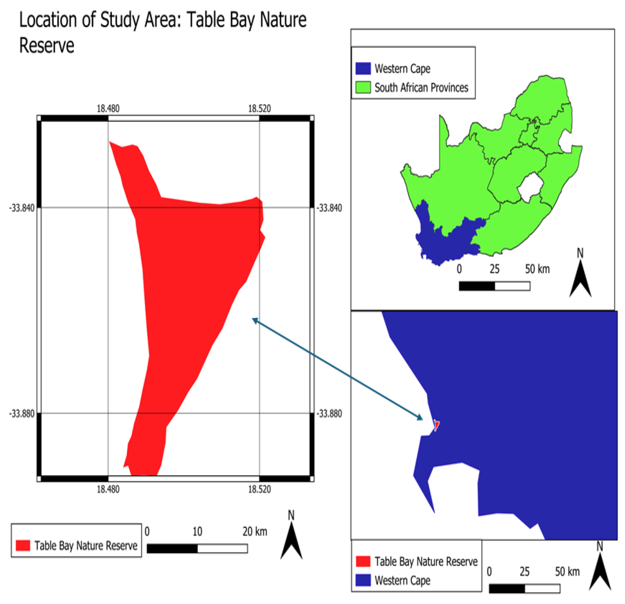
The study was conducted in the Table Bay Nature Reserve located in Milnerton, City of Cape Town, Western Cape (Figure 1). The reserve is a critical ecological site located along Cape Town’s western coastline at approximately 33°50′45″ S, 18°30′01″ E (−33.84579, 18.50039). It is a vital link between Cape Town’s city center and the Cape West Coast Biosphere Reserve [13]. It is situated within a densely populated metropolitan area (City of Cape Town) that has over 3.7 million people and covers an area of about 880 hectares. The reserve experiences a temperate mediterranean climate which is characterized by mild, wet winters and warm, dry summers with daytime temperatures ranging from 20 °C to 26 °C with occasional peaks over 30 °C. In winter the daytime temperatures can range from 12 °C to 17 °C. The reserve is also located approximately 25 km (about a 20 min drive) from one of the world’s seven wonders, Table Mountain [13].

The reserve constitutes seven smaller reserves, namely Rietvlei Wetland Reserve, Milnerton Lagoon, Milnerton Beach, Milnerton Racecourse Nature Reserve, Zoarvlei Wetlands, and Diep River Fynbos Corridor and Parklands Fynbos Corridors which were united in 2012 [24]. The Table Bay Nature Reserve is an essential green corridor amid urban development and is bordered by suburbs such as Milnerton, Bloubergstrand, Parklands, Table View, and the informal settlement of Dunoon [24].

The biodiversity over the years within the Table Bay Nature Reserve has provided habitats for species such as the Cape clawless otters, honey badgers, and the threatened African black oystercatchers, as well as biome-restricted species such as Cape spurfowl and Cape bulbul, among over 200 bird species such as the greater flamingos, African fish eagles, pelicans, and the endangered Damara tern [24]. The reserves diverse ecosystem has supported a wide range of flora with more than 400 plant species occurring such as the Cape Flats Dune Strandveld, Cape Flats Sand Fynbos, Cliffortia ericifolia, and Acrolophia bolusii that are increasingly vulnerable to urban pressures [13,24].

2.2. Data Acquisition and Processing

For the purpose of this study, Google Earth Engine (GEE) was used as it provides a repository of satellite imagery, including Landsat 5 TM, Landsat 7 ETM+, Landsat 8 OLI, and Sentinel-2, which were essential in assessing the land use/land cover (LULC) of the reserve over the 24-year period. Data can be accessed by using their respective collection IDs within the GEE platform (https://earthengine.google.com/).

A single random classifier was trained on the reference data from 2012, which was subsequently applied to all the study years in to ensure consistency in the detection of change. As shown in

Table 1. Satellite sensors and data products used for annual composite generation.

Target Year	Primary Sensors	GEE Data Collection	Temporal Range	Cloud Filter	Compositing Method
All Years (2000–2024)	Landsat 5 TM, Landsat 7 ETM+, Landsat 8 OLI	LANDSAT/LT05/C02/T1_L2 LANDSAT/LE07/C02/T1_L2 LANDSAT/LC08/C02/T1_L2	May 1–October 28 (each year)	Cloud cover ≤ 50% QA_PIXEL masking	Median
2016+	Sentinel-2 MSI	COPERNICUS/S2_SR_HARMONIZED	May 1–October 28 (each year)	Cloudy pixel % ≤ 50% QA60 masking	Median

, For each year, dry season composites (May–October) were generated by merging the available scenes from the Landsat collection imagery and the Sentinel-2 imagery collection.

2.3. The Preprocessing Data

Several key steps were undertaken to ensure data quality and comparability across the sensors for accurate mapping. One important step was cloud and shadow masking where for each image collection, pixels contaminated by clouds, cloud shadows, and atmospheric aerosols were masked using the quality assessment (QA) bands provided with the surface reflectance (SR) products. After this process only clear, real land surface data was left to be used for map generation. Another challenge that was observed during data acquisition was that in 2003, Landsat 7’s sensor experienced a fault where the Scan Line Corrector (SLC) broke. This meant that data acquired from this satellite after 2003 contained some data gaps. The SLC is essential because it is the part within the sensor that keeps it aligned and stabilized, allowing the sensor to scan the Earth’s surface in straight and even lines as it orbits [25]. To deal with this challenge, a focal mean interpolation algorithm was applied to these images to estimate the gaps using the average values of nearby pixels in order reconstruct the images and fill the gaps prior to analysis.

In order to avoid spectral inconsistency between Landsat 8/9 OLI and the earlier Landsat sensors 5 and 7 (TM, ETM+), the bandpass adjustments were made. The bands were aligned with the spectral response of the legacy sensors using established coefficients to minimize false signals in the change analysis [22]. For the analysis period, a cloud-free median composite was created to reduce residual noise or any atmospheric effects that may interfere with the images. All the cleared and masked scenes within the analysis period were combined and the median for each pixel was calculated.

Furthermore, the training samples were manually digitized using high-resolution basemaps available in Google Earth Pro; however, the precise acquisition dates and spatial temporal characteristics of the basemaps were not recorded.

2.3.1. Radiometric and Atmospheric Corrections

Before analyzing the satellite imagery, it is important to correct variations caused by the sensors and the atmosphere. Satellite sensors do not always measure the surface of the Earth perfectly, and in order to ensure that the satellite imagery accurately represents it, atmospheric and radiometric corrections were performed for this study. These corrections were made for the Landsat imagery and Sentinel-2 imagery. Radiometric corrections adjust for differences in sensor sensitivity and cross-calibrate data from multiple sensors, such as Landsat 7 and Landsat 8, to ensure that the surface reflectance values are comparable [26]. Atmospheric corrections were then performed to remove any distortions in the imagery caused by the air above the Earth’s surface so that the pixels can truly represent the land surface [27]. The corrections for Sentinel-2 and Landsat can be performed using methods such as the Pseudoinvariant Areas (PIA), which is a method that uses standardized measurements across the different sensors that allows for accurate comparisons [28]. However, for this study Landsat analysis-ready data as well as Sentinel-2 Level-2A data that were already corrected were used for analysis and LULC classification and change detection. All satellite imagery was resampled to a common 30 m spatial resolution grid before median composites were generated and subsequent analysis carried out, so that the multi-sensor time series would be consistent and comparable.

2.3.2. Calculation of Vegetation and Built-Up Indices

In order to enhance the discrimination between key land cover classes, special indices were calculated from the processed satellite imagery. These indices are important as they leverage the distinct spectral signatures of different surface materials which allows for robust inputs for the classification algorithm to be used [29]. The primary vegetation indicator that was used was the Normalized Difference Vegetation Index (NDVI), calculated as the normalized ratio of the near-infrared (NIR) and the red band. The NDVI is a well-established measure of life green vegetation biomass. Its values typically range from −1 to +1 and the higher values indicate a denser and healthier vegetation [30]. To further capture the spatial heterogeneity of vegetation canopies, a textural measure was developed from the NDVI. This was performed by applying a gray level co-occurrence matrix (GLCM) analysis with a 3 × 3 pixel kennel to the NDVI values which then resulted in an NDVI contrast band that ensured that local texture and pattern variation were quantified. The NDVI was calculated using the following formula:

$$\mathrm{NDVI}={\displaystyle \frac{NIR-Red}{NIR+Red}}$$

Next, we needed to identify the built-up surfaces and for this we used the Normalized Difference Built-Up Index (NDBI). This index is computed using the short-wave infrared (SWIR 1) 1 and the near-infrared (NIR) bands. The built-up materials such as concrete and asphalt show a higher reflection in the SWIR 1 region compared to vegetation. This leads to positive NDBI values for urban areas [31]. The separation between the oven fabric and other land cover classes was improved by a composite of the Urban Index (UI) being calculated by simply subtracting the NDVI from the NDBI. This enhanced pixels that exhibited areas with high built-up characteristics and low vegetation. Furthermore, the Normalized Difference Balance Index (NDBAL) was derived from the two SWIR bands which were used to distinguish soil and other non-vegetation surfaces. The NDBAL’s formula is as shown below:

$$DBAL={\displaystyle \frac{(SWIR2-SWIR1)}{(SWIR2+SWIR1)}}$$

The Modified Normalized Difference Water Index (MNDWI) [32] was used to help easily detect water bodies by removing disturbances on built-up and vegetation surfaces. The index was derived from the following:

$$\mathrm{MNDWI}={\displaystyle \frac{Greenband-SWIR1}{Greenband+SIWR1}}$$

This study refers to the green and SWIR bands as the short-wave infrared bands that have green and infrared wavelengths, respectively. A MNDWI value greater than 0.2 was used to classify pixels as water, based on empirical tests and visual comparisons with reference imagery and field observations. Additional constraints were applied to address spectral confusion: NDVI < 0.1 and NDBI < 0 pixels were used as final water candidates. To reduce misclassification caused by temporary moisture, flooded vegetation, or phenological changes, the MNDWI was applied to atmospherically corrected surface reflectance composites from the dry season. MNDWI has some limitations, such as its inability to distinguish turbid or shallow water, wet soils, shadowed areas, and bright sandy substrates, which can be misinterpreted as water. A manual verification and cross-check of NDVI and NDBI composites were conducted to mitigate these issues. Additionally, cloud-free scenes were selected within the same seasonal window to minimize the effect of illumination conditions and viewing geometry. Thus, the revised approach, rather than achieving perfect separation between classes, enhances the reliability of water body identification through multi-index filtering and contextual verification.

2.3.3. Topographic Predictors

The topographic predictors derived from the Shuttle Radar Topography Mission (SRTM) Digital Elevation Model (30 m resolution) were employed together with spectral and index-based factors. These were, among others, elevation, slope, and aspect, which are the key factors describing the terrain and hence, the differences in the areas regarding the vegetation, soil moisture, and settlement locations. Table S1 (Supplementary Materials) contains a complete list of all predictor variables including the following: spectral bands, indices, and topographic derivatives, as well as a data source, spatial resolution, and classification category information.

2.4. Random Forest Classification and Validation

In this study, a single Random Forest classifier was trained to perform the land cover classification for all years and across both satellites (Sentinel-2 and Landsat). The rationale for using one machine learning algorithm was to create a transferable and consistent model, which will ensure that the land cover changes that are detected over time are due to actual landscape alterations and not variation between different models. The initial training data consisted of 17 polygons, and the class distribution within these original polygons was water (4 polygons), vegetation (6 polygons), built-up areas (4 polygons), and bare land (3 polygons). The bare land class included naturally occurring dunes, exposed soils from seasonal wetlands and land surfaces degraded or exposed through anthropogenic activities. Once this was achieved, the polygon features were exported as a Keyhole Markup Language (KML) file and uploaded to Google Earth Engine as a feature collection asset for further processing and classifier training.

For the enhancement of the statistical robustness of the training data, each polygon was converted into multiple sample points. This was achieved by using a stratified sampling approach with 50 points being systematically generated within each polygon boundary. This then resulted in set of 850 training points that were distributed across all land cover classes. The study used training data which were derived from high-resolution reference imagery (Google Earth Pro) for supervised classification. To ensure temporal consistency with the multi-year Landsat composites, three distinct time periods were selected to effectively illustrate the various stages of land cover change: 2010, 2015, and 2023. High-resolution images from Google Earth, Sentinel-2 Level-2A, and PlanetScope were utilized based on their availability and quality. To minimize the impact of phenological and illumination differences, imagery for each epoch was acquired during the same seasonal window (dry season: May–September) as the Landsat scenes. Table 1 shows all images sources, i.e., dates of acquisition, spatial resolution, and cloud cover conditions. The digitation process was performed manually creating a polygon boundary of each land cover class (water, built-up, bare land, and vegetation) within the Table Bay Nature Reserve. Furthermore, using the visual homogenous areas confirmed through the spectral profiles and field validation. To improve representativeness and also to minimize spatial autocorrelation, polygons were converted into point samples, such that points were generated using a stratified random sampling with a minimum distance of 60 m between them. This was performed to ensure that points from the same polygon would not be considered as fully dependent observations. Points were then balanced between classes and periods such that each class and period contributed equally to the model training. Changes in land cover through time are unavoidable, but the use of multiple years of high-resolution satellite imagery, contemporaneous to the Landsat composites, has substantially improved temporal agreement between training and classification datasets. The Random Forest classifier was set to 300 trees and it was able to be used for the LULC classification. The main advantage of using a Random Forest classifier is its robustness and accuracy [33]. Since it builds an ensemble of many decision trees that are each trained on random subsets of both the data and input variables, it reduces the challenges such as overfitting the training data [33]. This makes it reliable for complex data such as satellite imagery, where spectral signatures of different land cover classes may overlap.

Model Validation and Accuracy Assessment

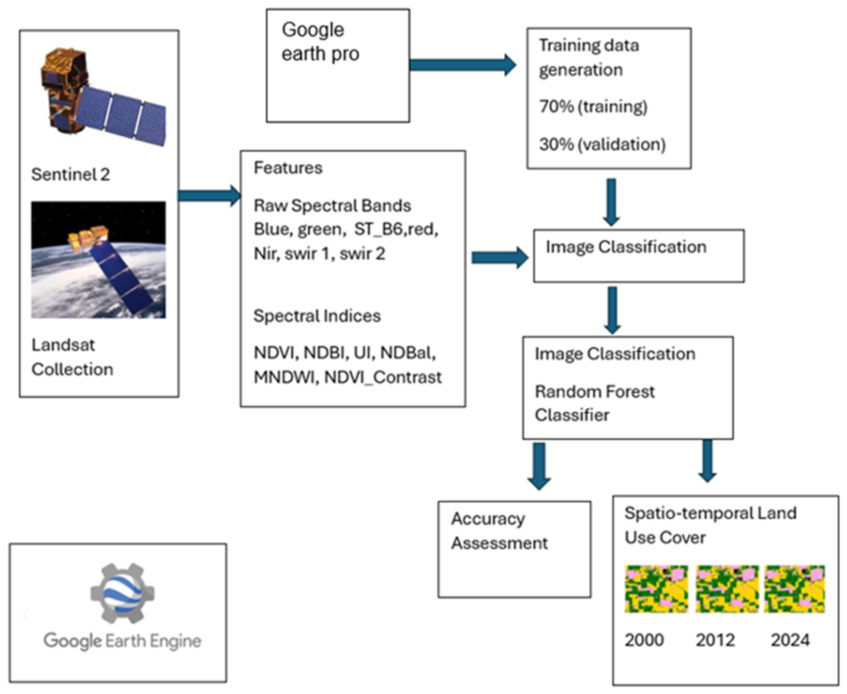
To evaluate the classifier’s performance, the 850-point dataset was randomly divided into two subsets: training (70%, 564 points) and independent validation (30%, 236 points). By splitting the training data into two subsets, the model was able to evaluate its accuracy on data that had not been seen during training. The accuracy assessment was conducted within the Google Earth Engine using a confusion matrix. The confusion matrix compared the classified pixel values against the ground truth validation dataset. From these matrices key statistical metrics were obtained which included the overall accuracy, the producer’s accuracy, the user’s accuracy, and the Kappa coefficient. Together these indicators provided a comprehensive evaluation of classification reliability by quantifying both the general agreement and the class specific accuracies. The flow chart provides a clear and systematic visualization of the methodology, outlining each key step involved in the process. (Figure 2).

3. Results

3.1. Relative Contribution of Spectral Features (Spectral Bands and Indices) in the Classification

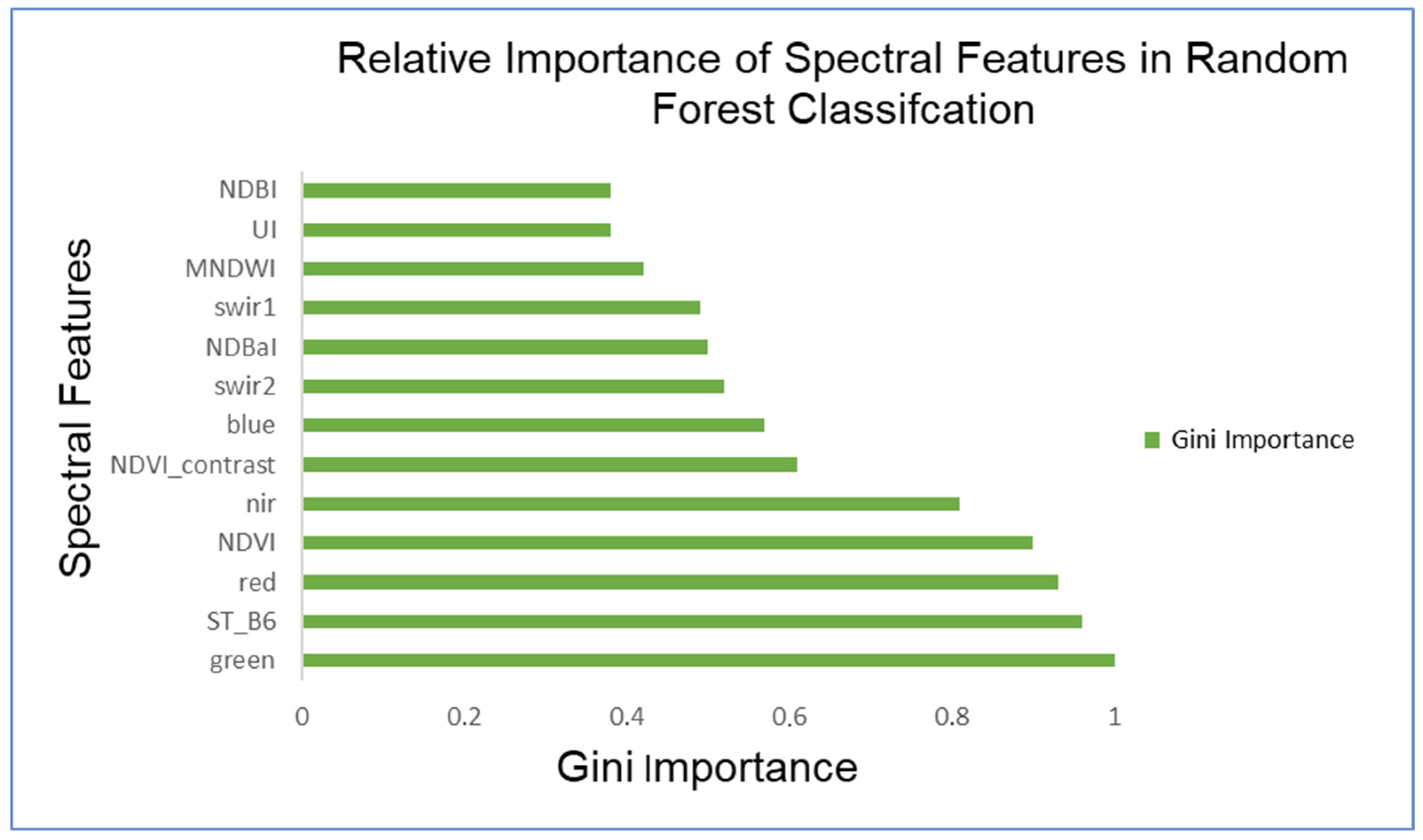
The random classifier provided estimates of feature importance, which reveals the relative contribution of each of the spectral bands and indices to the classification models decision-making process. The graph (Figure 3) below shows which satellite spectral bands and indices were the most useful for the model to correctly classify the classes of land. A higher score means the band or index was more important for the accuracy of the model. The most important variable was the simple green color band from the satellite.

This band is particularly sensitive to water turbidity, suspended sediments, and vegetation greenness, enabling it to effectively discriminate coastal and wetland surfaces from surrounding dry or sandy areas. In the reserve’s mixed dune–wetland environment, the green band captured subtle transitions between aquatic and terrestrial surfaces that other bands and indices could not fully resolve.

The strong contribution of the thermal band (ST_B6) demonstrated the critical role of land surface temperature in distinguishing land cover classes. Built-up and bare land surfaces exhibited elevated LST values due to reduced evapotranspiration and high heat absorption, while vegetation and water maintained lower temperatures. This pattern underscores the presence of a localized urban heat island effect and affirms LST as a valuable discriminant in mixed urban ecological settings.

The red and NDVI variables further contributed to the model by distinguishing vegetated from non-vegetated areas, while the relatively low importance of specialized indices (e.g., NDBI, UI, MNDWI) suggests that the fundamental spectral bands alone were sufficient for class separation in this heterogeneous coastal system. This implies that in areas with clear spectral contrast among land cover types, complex indices may provide limited additional discriminatory power.

3.2. Spatiotemporal Land Use Cover

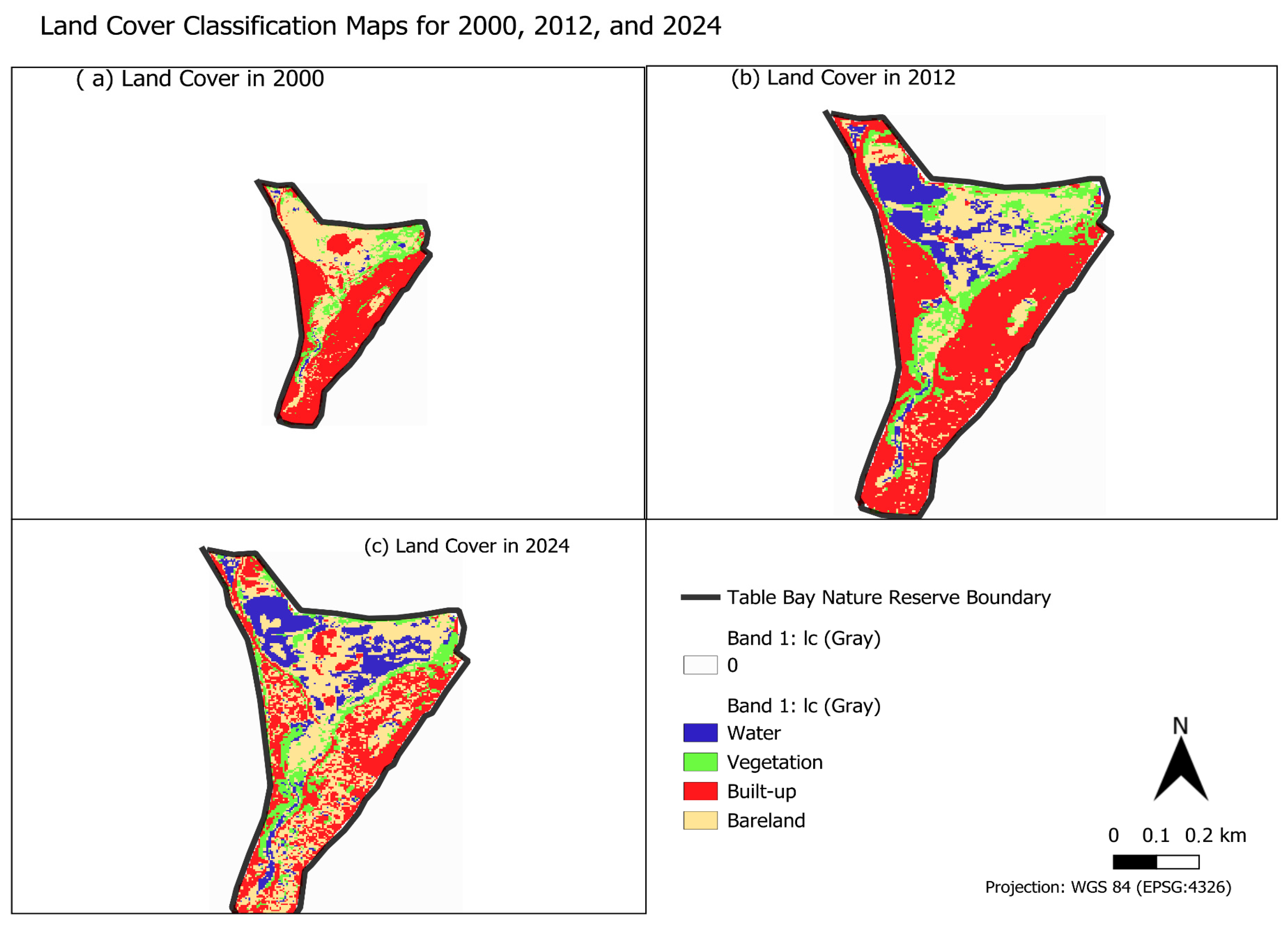
Between 2000 and 2024, the Table Bay Nature Reserve experienced shifts in land cover composition. The most substantial changes included a dramatic increase in water bodies, a notable decline in built-up areas, and moderate shifts in bare land and vegetation cover. The trend experiences are explored in detail through spatial and statistical analyses in Figure 4 and Figure 5, respectively.

Figure 4 visually confirms the major trends that were observed in the statistical analysis provided in Figure 5. The 2000 LULC (Figure 4a) map serves as a baseline representation of the pre-expansion condition of the Table Bay Nature Reserve. The most striking spatial change was the dramatic expansion of water bodies (shown in blue). In the year 2000 (Figure 4a), water can be seen confined to a few isolated pockets. By 2024, the water bodies had expanded significantly particularly in the northern region of Figure 4c.

In addition, the retreat of built-up areas (shown in red) is also evident in the maps. The 2000 and 2012 (pictured in A and B, respectively) maps show the extensive urban patches within the reserve. However, in 2024 (Figure 4c), there is a visible shrink and fragmentation of built-up areas. In the 2024 map, there is more visibility of bare land patches (indicated in tan) across the built-up patches (red). This expansion of bare land is consistent with the 41.3% decrease in built-up areas that is reported in Figure 5 and suggests possible transitional construction zones or cleared infrastructure. Vegetation (green) appeared fragmented and scattered throughout the study period, primarily along the wetland corridors and coastal margins, indicating the persistence of natural plant communities despite surrounding urban influence.

3.3. Understanding RF Feature Importance in LULC Assessment from 2000 to 2024

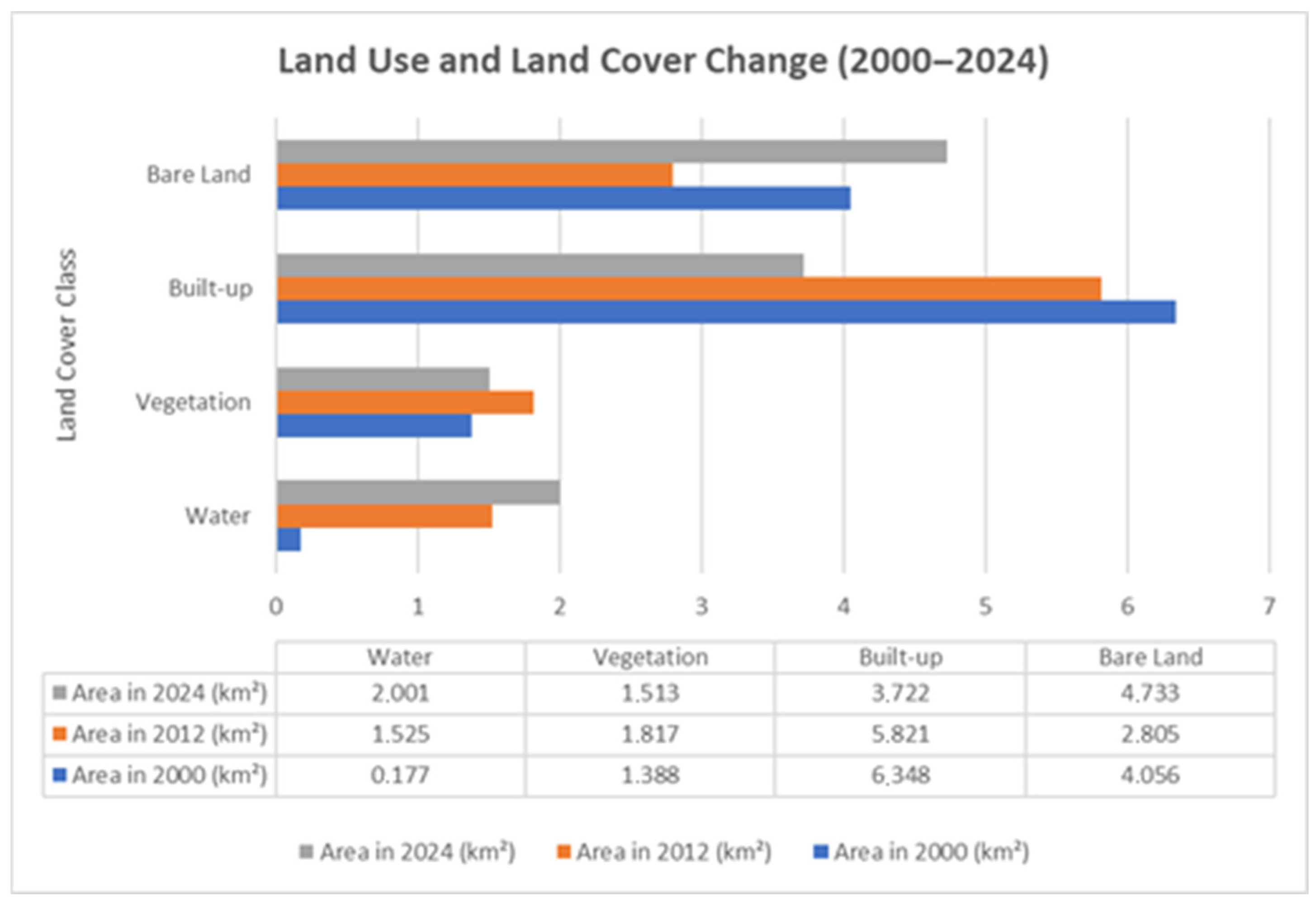
Figure 5 below shows the land use and land cover (LULC) dynamics within the Table Bay Nature Reserve between 2000 and 2024, derived from multi-temporal satellite imagery (Landsat 5 TM, Landsat 7 ETM+, Landsat 8 OLI, and Sentinel-2). The analysis focused on four dominant land cover classes, namely: water, vegetation, built-up, and bare land, in order to assess the effects of urban expansion on the reserve’s ecological integrity. According to Figure 5, water bodies increased substantially over the period from 0.18 km² in 2002 to 2.00 km² in 2024. This represented a 1030% increase, indicating that there was a dramatic expansion of water bodies within the reserve. Built-up areas experienced a decline from 6.35 km² in 2000 to 3.723 km² in 2024 showing a 41% reduction. This apparent reduction may not necessarily mean an actual decline in urban structures. It may result from improved classification accuracy using high-resolution Sentinel-2 data that better distinguishes between built-up and bare land. Nonetheless, the spatial proximity of built-up zones to the reserve boundary underscores ongoing urban pressure from surrounding suburbs and industrial developments in Cape Town’s northern corridor.

The vegetation cover pattern indicated that there were minor fluctuations, where there was an increase from 1.39 km² in 2000 to 1.82 km² in 2012. This increase was then followed by a decline to 1.51 km² in 2024. Despite this decline, the overall vegetation cover in 2024 remained higher than that of 2000, suggesting restoration of green areas over the years. Bare land increased from 4.056 km² in 2000 to 4.733 km² in 2024, suggesting progressive vegetation clearance, soil exposure, or construction-related disturbances. This trend aligns with the broader urban sprawl patterns observed around the reserve, where open spaces are being modified for infrastructure expansion, sand mining or any other informal activities.

3.4. Multi-Sensor Output Map and Accuracy Assessment

The Random Forest classifier produced an overall accuracy of 98.7% and a Kappa coefficient of 0.983. This means that there is an almost perfect agreement between the classified map and the ground truth validation data. The Kappa coefficient being that high confirms that this overall accuracy is not a result of random chance or a class imbalance. Sometimes high accuracy metrics like these may raise questions of potential overfitting, several factors mitigated this concern. Based on the results in

Table 2. Shows the accuracy assessment of the producer’s accuracy and user’s accuracy.

class_id	Class Name	f1_score	User Accuracy (UA)	Producer Accuracy (PA)
0	Water	0.99	1	0.982
1	Vegetation	0.987	0.987	0.987
2	Built-up	0.982	0.982	0.982
3	Bare land	0.98	0.978	1

, water was classified with exceptional precision. The user’s accuracy of 1.0 showed that every pixel classified as water was accurate, while the producer’s accuracy of 0.982 showed that nearly all the water pixels were successfully captured. When it comes to the vegetation and built-up areas, they showed a perfectly balanced accuracy (UA and PA of 0.987 and 0.982, respectively), showing a minimal error rate for these two classes.

Bare land was mapped with perfect sensitivity, as shown by a producer’s accuracy of 1.0. This means that the actual bare land pixels were captured correctly by the model. However, the slightly lower user’s accuracy of 0.978 suggests that there could have been a minor overestimation, suggesting that a small number of pixels for the other classes might have been misclassified as bare land. However, these small misclassifications are common and are expected in remote sensing, as there are almost always some commission errors in modeling due to similarities between the classes [34].

3.5. Urban Expansion and Land Cover Change (2000–2024)

Between 2000 and 2024, there has been substantial urban expansion with the reserve which reflected the increasing footprint of urban areas and encroachment within the reserve. The analysis of land use and land cover (LULC) revealed significant transformations within the Table Bay Nature Reserve and its surrounding buffer zones (

Table 3. Raw encroachment metrics.

expansion_km2	Zone
0.3238979528588393	Inside Reserve
0.008002975806382123	1–5 km ring
0.0	5–10 km ring

and

Table 4. Percent change in area per class between 2000 and 2024.

Land Cover Class	Change 2000–2024 (km2)	Percent Change (%)
Water	1.824	1030
Vegetation	0.125	9
Built-up	−2.626	−41.3
Bare Land	0.677	16.7

; Figure 6).

3.6. Urban Encroachment into the Reserve

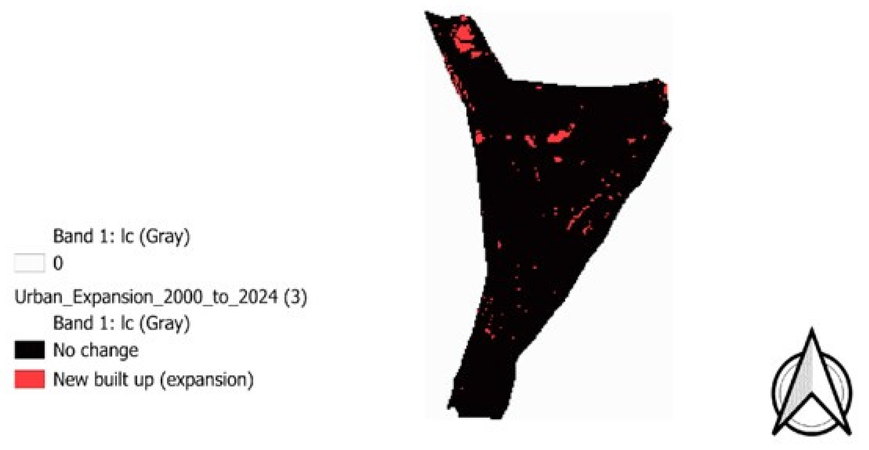
Urban encroachment analysis (Table 3) indicates that approximately 0.324 km² of built-up area expanded directly within the reserve boundary, highlighting a measurable degree of infringement into protected zones. In contrast, the surrounding buffer zones (1–5 km and 5–10 km rings) showed minimal additional expansion, suggesting that the most critical urban pressure is localized within the reserve itself rather than its immediate surroundings. The spatial distribution illustrated in Figure 6 confirms this pattern, with built-up areas increasingly penetrating the reserve (indicated in red), particularly along its southern and eastern boundaries adjacent to the Blouberg and Milnerton urban complexes. This expansion not only reduces available habitat for native species but also fragments ecological corridors, diminishing the reserve’s overall resilience.

3.7. Land Cover Transitions (2000–2024)

As indicated in Table 4, the most notable change occurred in water bodies, which increased by 1.824 km² (1030%), indicating substantial hydrological modification, possibly linked to enhanced stormwater management infrastructure, expansion of wetland habitats, or prolonged seasonal inundation events. Vegetation cover experienced a modest increase of 0.125 km² (9%), reflecting limited natural regeneration and localized rehabilitation within the reserve.

Conversely, built-up areas exhibited a significant reduction of 2.626 km² (−41.3%) over the 24-year period. Although this may suggest a decline in impervious surface area, the observed change likely reflects improved land cover classification accuracy and re-allocation of mixed-use or disturbed zones to bare land or vegetation classes in later datasets. Bare land, meanwhile, expanded by 0.677 km² (16.7%), which may be attributed to continued land disturbance, sand exposure, and degradation of vegetated surfaces due to anthropogenic activity and adjacent urban expansion.

The spatial distribution of changes shown in the expansion map (Figure 6) complements the quantitative analysis (Table 3 and Table 4) of the urban expansion. The expansion that occurred within the reserve itself is visually shown by the red patches in Figure 6 as new built-up regions.

4. Discussion

4.1. Urban Expansion Within the Reserve from 2000 to 2024

Although the newly developed built-up area within the reserve measures 0.324 km², it constitutes approximately 3.7% of the Table Bay Nature Reserve, which encompasses an area of approximately 880 hectares (8.8 km²). While this expansion may seem relatively minor in absolute terms, it holds ecological significance. The introduction of small-scale urban development within a protected area affects habitats and disrupts sensitive ecosystems, ultimately impacting the biodiversity within the reserve. This data indicates that informal settlements have directly intruded into the reserve area rather than being the result of slow encroachment from nearby regions, based on eviction records and land use data from the Diep River floodplain.

However, it is located in a protected ecological zone, which indicates that the habitat has been disturbed and lost. This estimate is subject to uncertainty due to potential errors in classification and georeferencing, seasonal changes, and edge effects; therefore, it should be viewed as a rough indicator rather than a statistical test. This indicates that urban encroachment is affecting the protected area and has undermined the reserve’s conservation objectives and the supporting services they offer over the years. This is particularly concerning because even the smallest increases in built-up areas have effects in critical areas that are ecologically sensitive. Despite the broader LULC analysis showing an overall decline of 41.3% in built-up areas between 2000 and 2024, the assessment of the expansion within the reserve highlights that there has been localized urban growth within the TBNR boundary over the 24-year period. This seems contradictory between the LULC assessment and the reserves urban expansion assessment, suggesting that while the regional built-up areas may have been reduced or reclassified into other categories, such as water or vegetation, most likely due to reclamation of abandoned urban areas over the years. The reserve nevertheless experienced urban expansion from 2000 to 2024.

Similar trends of urban expansion have been observed globally. For instance, a study by Aljoufie et al. [35] examined the decadal land cover changes in Al-Khobar, Saudi Arabia. This study used remote sensing and GIS tools, and a consistent outward expansion of built-up areas between the study period was witnessed. Their study illustrated the importance and reliability of using remote sensing GIS in monitoring urban expansion/encroachment. Furthermore, in their study, Mundia and Aniya [36] showed a 47 km expansion of urban areas in Nairobi, Kenya, which was driven by the proximity of the areas to road networks and the growth of the economy. The findings of these studies motivated the use of remote sensing and GIS technologies in monitoring urban expansion in the TBNR. By applying a similar methodological approach in detecting the localized urban encroachment within a protected area, a consistent trend of urban expansion of urban areas was identified with the reserve and with the increase of urbanization. The results of this present study contribute to the globally witnessed trend of urban expansion as a result of global urbanization rates.

4.2. Ecological Implications of Urban Sprawl in Cape Town Table Bay Nature Reserve

The observed LULC shifts do have ecological implications. For example, the expansion of the water bodies as witnessed can enhance the availability of habitats and therefore ensure biodiversity within the reserve is sustained by ensuring the well-being of aquatic and bird species is maintained. This increase could be attributed to factors such as improved wetland management, construction of artificial ponds or perhaps shifts in rainfall patterns. However, in the case of the increase in bare land spaces, the implications may not be as positive. Impacts such as erosion risks can be experienced, which may ultimately lead to habitat degradation, placing pressure on species that are not able to adapt if these impacts are left unmanaged. Additionally, the fact that the urban expansion that was experienced by the reserve was more concentrated within the reserve itself than the 0–10 km buffer zones was concerning because this means the impact on biodiversity within the reserve was exacerbated. This encroachment has led to notable ecological and landscape transformations due to the unchecked expansion of urban areas in its undeveloped landscapes [13]. Such transformations reduce the size of habitats, which then leads to the creation of more fragmented, smaller habitat patches that are isolated. This impacts biodiversity because, due to these isolated patches, species movement and gene flow are limited. This increases the vulnerability of the smaller species populations within the reserve.

The increased human activity within the reserve also exerts pressure on the ecological balance of the system. The activities introduce impacts such as pollution, particularly water pollution due to increased runoff that carries solid waste in water spaces. As a result, the ecological integrity of the reserve is compromised and its resilience to environmental stressors is reduced [1]. Similarly to this study, other studies at a global scale have consistently found that urban expansion causes habitat loss and fragmentation ultimately leading to biodiversity degradation [7]. In their study, the authors used present and future spatial projections to assess how urban expansion causes significant natural habitat loss and biodiversity decline globally, especially in restricted biodiversity hotspots in sub-Saharan Africa. This study provided a strong foundation that aligns with the observations from this present study, that urban sprawl inside restricted/protected areas causes significant habitat fragmentation and biodiversity loss.

It is important to be aware that declaring areas as protected can sometimes ensure it resists urban encroachment to some degree. For example, a study by Wang et al. [37] reported that protected areas in China effectively resisted approximately 33% of urban expansion, which suggests a certain level of success in conservation strategies for biodiversity in protected areas. However, this resistance is not always guaranteed in protected areas and varies with the effectiveness of the management strategies that are put in place within the protected area. In the TBNR study, the concentrated urban expansion within this protected reserve suggests that the conservation strategies may be limited or enforcement measures are weak. Hence, the reserve has not been able to resist urban expansion over the years.

5. Limitations

The most significant limitation of this study stems from the broad definitions of the classes. For instance, the ambiguous definition of the bare land class, which likely encompasses both natural features and anthropogenic surfaces (e.g., disturbed soil), complicates the interpretation of its increase. It may be a primary factor in the observed large-scale decrease in the built-up class, as improved sensor resolution may have led to the reclassification of previously misclassified pixels.

Moreover, while the land cover-based approach used in this study was effective for detecting spatial change, it cannot discern the ecological conditions or quality. For instance, the vegetation class does not distinguish between native fynbos or invasive species, and the water class does not differentiate between healthy or degraded wetlands, as well as natural or artificial water bodies. This limits the precision in the ecological interpretation of the findings.

Another limitation is the concern with the high classification accuracy of 98.7% which reflects a strong performance against the training data; however, the ambiguous class definitions and reliance on a single basemap introduce potential limited ecological precision. For this study, the GEE allowed for an efficient large-scale LULC analysis across the TBNR with high accuracy. However, the Landsat 30 m spatial resolution sometimes limits the detection of fine-scale habitat features that may have contributed to the minor classifications of other classes as bare land. Some of these errors could not be avoided due to the similarities the classes share. Another limitation that was noticed was when it comes to Sentinel-2 imagery, the imagery is available from 2015, making it impossible to solely depend on it for the monitoring of LULC over a large time period. Even though Sentinel-2 offers a finer spatial resolution of about 10–20 m, which could have been beneficial for this study, its shorter temporal coverage meant we could not overly rely on it for classification alone for the study period. Furthermore, a full transition matrix between the classes was not generated, and because of this, the precise directions of transformations and their reliability cannot be fully assessed. However, the classification accuracy metrics still provide a reliable indication of the land cover changes.

Despite these challenges, the benefits offered by GEE and the Random Forest classifier outweigh the challenges, as we were able to create LULC outputs for the study period that allowed us to quantify urban encroachment into the reserve.

6. Conclusions

This study investigated the impacts of urban sprawl on the natural landscape within the reserve using remote sensing tools, in particular Google Earth Engine. The impact was assessed by monitoring the land cover/land use change from 2000 to 2024. The most ecologically significant finding was the direct encroachment of approximately 0.324 km² of newly built-up area within the reserve. The results showed that encroachment occurred primarily within the reserve boundaries rather than the surrounding buffer zones, suggesting an increased pressure on sensitive ecosystems and biodiversity within the reserve. These results confirmed the vulnerability of protected areas faced with unregulated development. This context raises critical questions about the efficacy of existing policies and conservation strategies in mitigating urban pressure within the reserve. Preliminary observations suggest complex land cover dynamics may be at play within the TBNR, including potential fluctuations in vegetation and water bodies, warranting a detailed investigation. However, the growth of these classes must be interpreted with caution because they could also reflect anthropogenic alterations such as the introduction of invasive vegetation spread or artificial hydrological changes. Future field monitoring is needed to determine the contribution factors to the growth of the vegetation and water bodies.

The expansion of the bare land witnessed suggests an ongoing ecological degradation, while the built-up areas showed an unexpected decrease, which suggests that there is a possible land use reclassification or rehabilitation process within the nature reserve.

The combination of these results suggests that while the result from the urban expansion means that the most immediate impact is within the TBNR, the ecological responses to this have not been uniform as the study reveals a complex pattern of land cover transformation that has been marked by the redefinition of urban fabric, the emergence of new built-up areas and shifts in the bare land and vegetation classes. This transformation suggests both intrusion into the ecologically sensitive zones and potential reclassifications or clearance of older urban areas. This underscores the importance of continuous ecological monitoring to be able to differentiate between genuine restoration and ecologically harmful transformations. The findings present a dual narrative where measurable encroachment is posing a threat to habitat connectivity while significant landscape fluidity complicates linear interpretation of urban growth.

These results highlight the fact that there is a need for stricter enforcement of conservation measures and management strategies that prioritize biodiversity conservation amidst the precious experience as a result of urban growth. These findings showed a persistent trend of urban encroachment and ecological alteration within Table Bay Nature Reserve. Although some wetland and vegetative recovery is evident, the continuing conversion of natural and semi-natural areas into built-up or bare land poses serious challenges to conservation objectives. Furthermore, the water expansion observed in this study was of particular significance and therefore warrants further investigations in order to determine the driving force of this expansion and assess alignment with the reserves conservation efforts. These findings are relevant to the implementation of Sustainable Development Goal 15. The inability to distinguish between ecologically functional and degraded land cover classes underscores the importance of integrating ecosystem condition assessments into spatial planning. These findings support the need for improved monitoring frameworks that incorporate ecosystem values into local development strategies, as called for under SDG 15.9. Conservation strategies must be spatially explicit and focus on enforcement in the identified zones of encroachment while initiating detailed ground truthing studies to determine the ecological drivers behind the land cover transitions.

References

1. Yang, Y.; Erskine, P.D.; Lechner, A.M.; Mulligan, D.; Zhang, S.; Wang, Z. Detecting the dynamics of vegetation disturbance and recovery in surface mining area via Landsat imagery and LandTrendr algorithm. J. Clean. Prod. 2018, 178, 353–362. [Google Scholar] [CrossRef] [Scilit]
2. Al Tarawneh, W.M. Urban sprawl on agricultural land (literature survey of causes, effects, relationship with land use planning and environment): A case study from Jordan (Shihan Municipality Areas). J. Environ. Earth Sci. 2014, 4, 97–124. [Google Scholar]
3. Seto, K.C.; Fragkias, M.; Güneralp, B.; Reilly, M.K. A meta-analysis of global urban land expansion. PLoS ONE 2011, 6, e23777. [Google Scholar] [CrossRef] [Scilit]
4. Grangxabe, X.S.; Maphanga, T.; Chidi, B.S. Urban Nature Reserves Waste Challenges from Neighboring Informal Settlements: Western Cape, South Africa. Nat. Environ. Pollut. Technol. 2024, 23, 1483–1494. [Google Scholar] [CrossRef] [Scilit]
5. Ayeni, A.O.; Aborisade, A.G.; Onuminya, T.O.; Soneye, A.S.; Ogundipe, O.T. Urban development in Africa and impact on biodiversity. Curr. Landsc. Ecol. Rep. 2023, 8, 73–89. [Google Scholar] [CrossRef] [Scilit]
6. Shi, J.; Gong, J.; Zhang, Y.; Kan, G. Spatiotemporal change in ecological quality of the Qinghai-Tibetan Plateau based on an improved remote sensing ecological index and Google Earth Engine platform. Environ. Monit. Assess. 2025, 197, 1–20. [Google Scholar] [CrossRef] [Scilit]
7. Simkin, R.D.; Seto, K.C.; McDonald, R.I.; Jetz, W. Biodiversity impacts and conservation implications of urban land expansion projected to 2050. Proc. Natl. Acad. Sci. USA 2022, 119, e2117297119. [Google Scholar] [CrossRef] [Scilit]
8. McHale, M.R.; Bunn, D.N.; Pickett, S.T.; Twine, W. Urban ecology in a developing world: Why advanced socioecological theory needs Africa. Front. Ecol. Environ. 2013, 11, 556–564. [Google Scholar] [CrossRef] [Scilit]
9. He, J.; Bao, C.K.; Shu, T.F.; Yun, X.X.; Jiang, D.; Brown, L. Framework for integration of urban planning, strategic environmental assessment and ecological planning for urban sustainability within the context of China. Environ. Impact Assess. Rev. 2011, 31, 549–560. [Google Scholar] [CrossRef] [Scilit]
10. Grangxabe, X.S.; Maphanga, T.; Madonsela, B.S. Public participation on waste management between nature reserves and surrounding informal settlement: A review. J. Air Waste Manag. Assoc. 2023, 73, 589–599. [Google Scholar] [CrossRef] [Scilit]
11. Anderson, P.M.; Avlonitis, G.; Ernstson, H. Ecological outcomes of civic and expert-led urban greening projects using indigenous plant species in Cape Town, South Africa. Landsc. Urban Plan. 2014, 127, 104–113. [Google Scholar] [CrossRef] [Scilit]
12. Rebelo, A.G.; Boucher, C.; Helme, N.; Mucina, L.; Rutherford, M.C. Fynbos biome 4. In The Vegetation of South Africa, Lesotho and Swaziland; South African National Biodiversity Institute (SANBI): Pretoria, South Africa, 2006; pp. 144–145. [Google Scholar]
13. City of Cape Town. Integrated Reserve Management Plan: Table Bay Nature Reserve; Environmental Resource Management Department: Cape Town, South Africa, 2011. Available online: https://resource.capetown.gov.za/documentcentre/Documents/City%20strategies,%20plans%20and%20frameworks/Table_Bay_IRMP_Jun2011v02_Final.pdf (accessed on 13 April 2025).
14. Wang, D.; Xu, P.Y.; An, B.W.; Guo, Q.P. Urban green infrastructure: Bridging biodiversity conservation and sustainable urban development through adaptive management approach. Front. Ecol. Evol. 2024, 12, 1440477. [Google Scholar] [CrossRef] [Scilit]
15. Weng, Q. Remote sensing of impervious surfaces in the urban areas: Requirements, methods, and trends. Remote Sens. Environ. 2012, 117, 34–49. [Google Scholar] [CrossRef] [Scilit]
16. Zhang, Q.; Zhang, H.; Zhao, D.; Cheng, B.; Yu, C.; Yang, Y. Does urban sprawl inhibit urban eco-efficiency? Empirical studies of super-efficiency and threshold regression models. Sustainability 2019, 11, 5598. [Google Scholar] [CrossRef] [Scilit]
17. Zhu, D.; Chen, T.; Zhen, N.; Niu, R. Monitoring the effects of open-pit mining on the eco-environment using a moving window-based remote sensing ecological index. Environ. Sci. Pollut. Res. 2020, 27, 15716–15728. [Google Scholar] [CrossRef] [Scilit]
18. Li, S.; He, Y.; Xu, H.; Zhu, C.; Dong, B.; Lin, Y.; Si, B.; Deng, J.; Wang, K. Impacts of urban expansion forms on ecosystem services in urban agglomerations: A case study of Shanghai-Hangzhou Bay urban agglomeration. Remote Sens. 2021, 13, 1908. [Google Scholar] [CrossRef] [Scilit]
19. Furberg, D.; Ban, Y.; Nascetti, A. Monitoring of urbanization and analysis of environmental impact in Stockholm with Sentinel-2A and SPOT-5 multispectral data. Remote Sens. 2019, 11, 2408. [Google Scholar] [CrossRef] [Scilit]
20. Shao, Z.; Sumari, N.S.; Portnov, A.; Ujoh, F.; Musakwa, W.; Mandela, P.J. Urban sprawl and its impact on sustainable urban development: A combination of remote sensing and social media data. Geo-Spat. Inf. Sci. 2020, 24, 241–255. [Google Scholar] [CrossRef] [Scilit]
21. Jiao, P.; Xing, C.; Li, Y.; Ji, X.; Tan, W.; Li, Q.; Liu, H.; Liu, C. A dataset of ground-based vertical profile observations of aerosol, NO2 and HCHO from the hyperspectral vertical remote sensing network in China (2019–2023). Earth Syst. Sci. Data 2024, 17, 3167–3187. [Google Scholar] [CrossRef] [Scilit]
22. Zhu, D.; Chen, T.; Wang, Z.; Niu, R. Detecting ecological spatial-temporal changes by Remote Sensing Ecological Index with local adaptability. J. Environ. Manag. 2021, 299, 113655. [Google Scholar] [CrossRef] [Scilit] [PubMed]
23. Zhang, Z.; Liu, X.; Li, J.; Fu, S.; Sun, Y.; Qiao, R. Analysis of spatiotemporal characteristics and influencing factors of land urbanization level in China at different scales based on nighttime light remote sensing. IEEE J. Sel. Top. Appl. Earth Obs. Remote Sens. 2024, 17, 9811–9827. [Google Scholar] [CrossRef] [Scilit]
24. Retief, J.J. Integrated reserve management plan, Table Bay Nature Reserve. In Environmental Resource Management Department—Biodiversity Management Branch; Cape Nature Reserve: Cape Town, South Africa, 2011. [Google Scholar]
25. Brown, C.W.; Connor, L.N.; Lillibridge, J.L.; Nalli, N.R.; Legeckis, R.V. An introduction to satellite sensors, observations and techniques. In Remote Sensing of Coastal Aquatic Environments: Technologies, Techniques and Applications; Springer: Dordrecht, The Netherlands, 2005; pp. 21–50. [Google Scholar]
26. Mishra, N.; Haque, M.O.; Leigh, L.; Aaron, D.; Helder, D.; Markham, B. Radiometric cross calibration of Landsat 8 operational land imager (OLI) and Landsat 7 enhanced thematic mapper plus (ETM+). Remote Sens. 2014, 6, 12619–12638. [Google Scholar] [CrossRef] [Scilit]
27. Richter, R.; Wang, X.; Bachmann, M.; Schläpfer, D. Correction of cirrus effects in Sentinel-2 type of imagery. Int. J. Remote Sens. 2011, 32, 2931–2941. [Google Scholar] [CrossRef] [Scilit]
28. Padró, J.C.; Pons, X.; Aragonés, D.; Díaz-Delgado, R.; García, D.; Bustamante, J.; Pesquer, L.; Domingo-Marimon, C.; González-Guerrero, Ò.; Cristóbal, J.; et al. Radiometric correction of simultaneously acquired Landsat-7/Landsat-8 and Sentinel-2A imagery using pseudoinvariant areas (PIA): Contributing to the Landsat time series legacy. Remote Sens. 2017, 9, 1319. [Google Scholar] [CrossRef] [Scilit]
29. Heiden, U.; Segl, K.; Roessner, S.; Kaufmann, H. Determination of robust spectral features for identification of urban surface materials in hyperspectral remote sensing data. Remote Sens. Environ. 2007, 111, 537–552. [Google Scholar] [CrossRef] [Scilit]
30. Huang, S.; Tang, L.; Hupy, J.P.; Wang, Y.; Shao, G. A commentary review on the use of normalized difference vegetation index (NDVI) in the era of popular remote sensing. J. For. Res. 2021, 32, 1–6. [Google Scholar] [CrossRef] [Scilit]
31. Kaur, R.; Pandey, P. A review on spectral indices for built-up area extraction using remote sensing technology. Arab. J. Geosci. 2022, 15, 391. [Google Scholar] [CrossRef] [Scilit]
32. Xu, H. Modification of normalised difference water index (NDWI) to enhance open water features in remotely sensed imagery. Int. J. Remote Sens. 2006, 27, 3025–3033. [Google Scholar] [CrossRef] [Scilit]
33. Salman, H.A.; Kalakech, A.; Steiti, A. Random forest algorithm overview. Babylon. J. Mach. Learn. 2024, 2024, 69–79. [Google Scholar] [CrossRef] [Scilit]
34. Khatami, R.; Mountrakis, G.; Stehman, S.V. Predicting individual pixel error in remote sensing soft classification. Remote Sens. Environ. 2017, 199, 401–414. [Google Scholar] [CrossRef] [Scilit]
35. Aljoufie, M.; Zuidgeest, M.; Brussel, M.; van Vliet, J.; van Maarseveen, M. A cellular automata-based land use and transport interaction model applied to Jeddah, Saudi Arabia. Landsc. Urban Plan. 2013, 112, 89–99. [Google Scholar] [CrossRef] [Scilit]
36. Mundia, C.N.; Aniya, M. Analysis of land use/cover changes and urban expansion of Nairobi city using remote sensing and GIS. Int. J. Remote Sens. 2005, 26, 2831–2849. [Google Scholar] [CrossRef] [Scilit]
37. Wang, N.; Du, Y.; Liang, F.; Yi, J.; Qian, J.; Tu, W.; Huang, S.; Luo, P. Protected areas effectively resisted 33.8% of urban development pressures in China during 2000–2018. Appl. Geogr. 2023, 159, 103079. [Google Scholar] [CrossRef] [Scilit]
Figure 1. A map showing where the Table Bay Nature Reserve is situated in Western Cape, South Africa.
Urbansci 10 00149 g001
Figure 2. Shows the summary of the methodology using a flow chart.
Urbansci 10 00149 g002
Figure 3. Variable importance from Random Forest classification.
Urbansci 10 00149 g003
Figure 4. Spatiotemporal patterns of land use and land cover change within the Table Bay Nature Reserve from 2000 to 2024 with a 12-year interval. (a) Land cover 2000; (b) Land cover 2012; (c) Land cover 2024.
Urbansci 10 00149 g004
Figure 5. Shows LULC area change between the years 2000 and 2024; the analysis of land cover change over the 24-year period reviewed significant shifts in the landscape.
Urbansci 10 00149 g005
Figure 6. Urban expansion within the Table Bay Nature Reserve between 2000 and 2024.
Urbansci 10 00149 g006