Spatiotemporal Analysis of Thermal Environment and Land Use Change in Sonipat, Panipat, and Jhajjar Districts Under the Central Circle Forest Area of Haryana, India (1993–2023)

Abstract

Changes in land use patterns due to urbanisation impact local weather patterns by influencing Land Surface Temperatures (LSTs). Despite rapid urbanisation in the Delhi-NCR (National Capital Region), the peri-urban fringes of Haryana, such as the Central Circle Forest (CCF) region, in the past three decades, a comprehensive 30-year analysis that integrates LST, the Normalised Difference Vegetation Index (NDVI), the Normalised Difference Built-up Index (NDBI), and Land Use/Land Cover (LULC) is lacking. The current study on the decadal analysis covering the 1993 to 2023 time period shows an increase in built-up areas (14.6–38.4%), a decline in NDVI (−0.01 to −0.08), a 6 °C rise in summer LST, and weak correlations between LST and NDVI. A significant increase in summer mean LSTs was observed, with some regions reaching temperatures beyond 35 °C in the selected districts. The LST and LULC zonal statistics revealed that the open fields/agricultural land and floodplains of the Yamuna River have adversely affected the weather pattern with rising LST. The average NDVI declined from −0.01 in 1993 to −0.08 in 2023, indicating a loss of vegetative buffers. Meanwhile, NDBI trends from 2003 to 2023 showed that built-up areas have steadily grown, and LULC data highlighted 38.43% of the built-up area in 2023. Correlation analysis showed a weak negative relationship between LST and NDVI (r = −0.47), suggesting diminishing cooling effects of vegetation, while a weak positive correlation between LST and NDBI indicates that urban expansion is significantly contributing to the urban heat island effect. This study emphasises the need for green infrastructure, afforestation, and water conservation in urban planning frameworks to enhance climate resilience and ecological sustainability.

1. Introduction

Remote sensing (RS) and Geographic Information Systems (GISs) have been pivotal in urban climate research since the 1970s, particularly in assessing spatial changes in Land Use/Land Cover (LULC) and Land Surface Temperature (LST) and in addressing the challenges posed by urbanisation [1]. LST serves as a crucial environmental parameter, providing insights into soil characteristics and climatic conditions, heat distribution, thermal stress, and the urban heat island (UHI) effect [2,3]. The relationship among LST, spectral indices, and LULC elucidates how the thermal characteristics of various land cover types influence the overall thermal dynamics [4]. Globally, researchers have extensively used LST to understand the effect of changing vegetation patterns and the expansion of urban areas [5]. For instance, a report by the United Nations Population Fund estimates that we are currently experiencing the largest wave of urbanisation in history [6], driving large-scale conversions of natural landscapes to built-up areas [7]. This leads to the increased use of heat-absorbing materials, such as concrete and asphalt, altering regional heat dynamics and the emergence of UHIs [8]. The rapid transformation of land use disrupts heat storage, alters evaporation rates, and creates microclimate variations, emphasising careful urban planning [9]. Regardless of extensive reporting of UHIs in temperate and developed cities (e.g., London +5–7 °C, New York +3 °C), developing nations and tropical regions remain notably under-studied [10]. African cities, such as Kampala (+2.5 °C UHI expansion encroaching on wetlands), tropical megacities, like Jakarta and Lagos (experiencing phenological delays), and South Asia (Delhi NCR +4.2 °C) [11] indicate absences of marginal forests in urban environments [12]. Elevated LST and UHI effects, driven by human activities and the built environment, can increase local temperatures by as much as 5 °C [13]. Cui et al. [14] found that every 10% increase in green cover resulted in a 0.39 °C decrease in mean LST, with larger Urban Green Spaces (UGSs) providing more pronounced cooling effects. It has already been reported that UGSs can mitigate some of these impacts by regulating temperatures and enhancing carbon sequestration [15]. The findings of Grigoras et al. [16] also illustrated the significant impact of LULC changes on UHIs, indicating a trend of increasing built-up areas at the expense of green spaces. Whereas the studies by Bala et al. [17] and Athokpam et al. [18] in India highlighted the critical need for future research in LST, the Normalised Difference Vegetation Index (NDVI), and the Normalised Difference Built-up Index (NDBI) in urban environments. Indices like NDVI and NDBI are studied as indicators of regional climate, whereas NDVI alone is insufficient for understanding LST and UHIs due to seasonal fluctuations in vegetation and open areas. This is why an LST, NDVI, NDBI, and LULC integrated study becomes necessary [1,17].

The available literature about Indian urban climate studies indicates that Delhi and cities near the National Capital Region (NCR) experience significant UHI effects of up to (+5 °C) due to the expansion of impervious surfaces surpassing green cover [13]. In Gurugram, Haryana, a significant transformation from vegetated to impervious surfaces has led to the strongest UHI effect observed in the region from the early 2000s to 2022 [19]. Prakash et al. [20] examined LST using Aqua MODIS data from 2003 to 2017, revealing that the average LST does not correlate with near-surface air temperature and that distinct land cover types exhibit varied temperature patterns. Shahfahad et al. [3] examined LST in four major cities of India (Chennai, Mumbai, Kolkata, and Delhi) using Landsat 8 data, highlighting how LST varied by city type. Coastal cities like Mumbai and Chennai exhibit moderated temperatures, while inland peri-urban areas, such as Chandigarh, reported a +2.5 °C increase in LST from comparable urban sprawl between 2016 and 2022 [21]. Similarly, a study by Imam et al. [22] discovered that inland towns, such as Pune, Bhopal, and New Delhi, experience more heat, while coastal cities, like Chennai and Visakhapatnam, benefit from moderating effects due to the sea. However, Mumbai faces the most severe heat intensities, likely due to pollution and high population density. This observation was further supported by other studies [2,4,23,24,25,26,27]. Goel [28] used satellite imagery to assess Haryana’s thermal environment and highlighted the substantial urban growth at the expense of arable land, which poses potential environmental risks. In a similar study, Agrawal et al. [21] observed a notable LST rise in Chandigarh, particularly in urban and barren areas, with an average increase of 2.5 °C from 2016 to 2022. In a separate study, Ramaiah et al. [29] compared two smart cities, namely, Panaji and Tumkur, in India and concluded that both water bodies and green spaces affect LST with varying effectiveness across different cities. In semi-arid Haryana, a longitudinal analysis for Hisar from 1991 to 2022 revealed increases in the minimum and maximum LST by approximately 20.4 °C and 17.2 °C [30]. The study noted the expansion of regional heat islands, driven by economic growth and land conversion to urban surfaces. These findings underline the strong correlation between urbanisation and thermal stress in Haryana’s semi-arid cities and highlight the need to examine similar dynamics in other NCR-proximate districts, such as the Central Circle Forest (CCF) region.

The Central Circle Forest (CCF) region of Haryana, adjacent to the NCR, one of the rapidly urbanising areas in India, is undergoing significant land use changes due to its proximity to the NCR [31]. This rapid transformation, driven by urban expansion, is exerting considerable pressure on its local environment, making it a key area of study for understanding the impacts of LULC changes and LST on regional climate dynamics [32]. There are no 30-year integrated analyses of LST, NDVI, and NDBI for the CCF region, where semi-arid vegetation degradation coincides with NCR expansion. The 30-year temporal window (1993–2023) was chosen not only for its length but also because it aligns with significant policy cycles and urbanisation periods in Haryana and the NCR sub-region. From 1991 to 2011, Haryana’s urban population nearly doubled, with the urbanisation rate increasing from 24.6% in 1991 to 34.8% in 2011, with over half of the State’s total urban population growth occurring over the decades of 1991–2001 and 2001–2011 [32]. This timeframe coincides with the implementation of the NCR Regional Plans 2001 and 2021, which advocated for decentralised growth corridors and industrial/transport infrastructure surrounding Delhi, hence directly impacting the expansion in Sonipat, Panipat, and Jhajjar [33]. Concurrent state-level initiatives, including HUDA/HSVP development plans, the establishment of Special Economic Zones (SEZs, such as the Gurugram–Jhajjar multi-service SEZs and petrochemical hubs in Panipat and Sonipat), along with successive Five-Year Plans and NITI Aayog strategies emphasising manufacturing and logistics, have significantly propelled the transformation of agricultural and forest land into developed areas in these districts [33]. Overlaying these demographic and policy changes is a recorded increase in regional temperatures and the frequency of heat waves in northwestern India during the same timeframe [30], rendering 1993–2023 a suitable period for evaluating policy-related land use transitions and their climatic manifestation in LST. The current research addresses three key elements in the context of RS and GIS for LST and LULC analysis: (1) scale: initial 30-year comprehensive analysis of CCF marginal vegetation during NCR expansion; (2) integrative analysis: concurrent NDVI-NDBI-LULC-LST explaining UHI mechanisms (e.g., diminished LST-NDVI correlations in semi-arid regions due to vegetation scarcity and anthropogenic heat); and (3) policy relevance: quantified vegetation loss and built-up increase directly correlates with Haryana’s smart city initiatives and climate action strategies for green infrastructure and afforestation initiatives. Hence, this study addresses these research gaps by examining integrated analyses of NDVI, NDBI, LST, and LULC in the three districts—Sonipat, Panipat and Jhajjar of CCF region of Haryana—with aims to i) assess changes in LST, built-up areas, and vegetation cover over time (1993–2023) in three districts of the CCF region of Haryana, India; ii) identify sensitive zones in terms of vegetation health and microclimatic changes by means of local-scale differences in NDVI, NDBI, and LST across several land use categories; and iii) assess spatial correlations between LST, NDBI, and NDVI across LULC categories to quantify urbanisation’s NDBI impacts on thermal patterns while accounting for vegetation’s NDVI moderation effects. This research will contribute to better urban planning and mitigating the environmental impacts of rapid urbanisation, particularly in developing countries.

2. Materials and Methods

2.1. Study Area

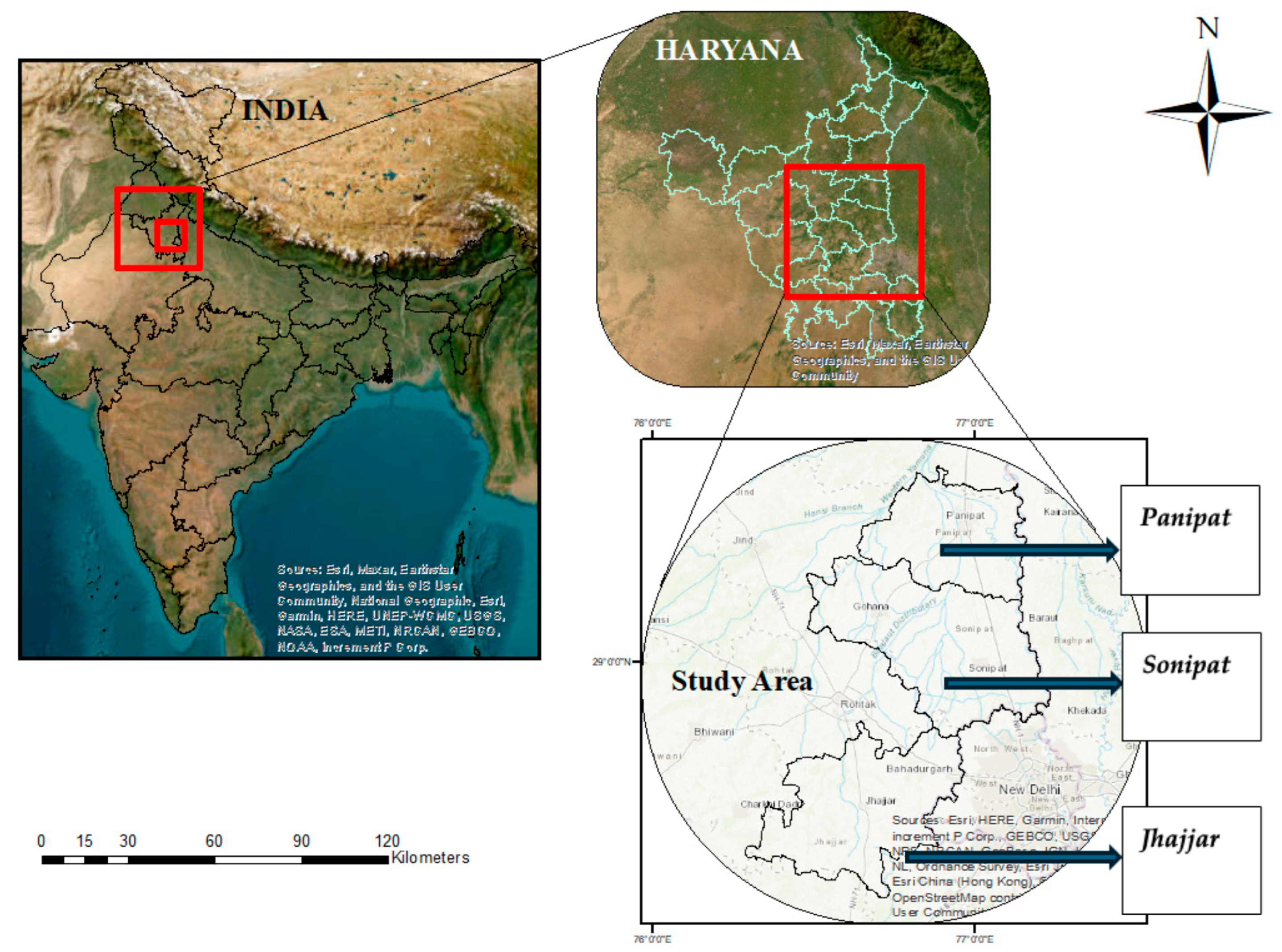
The present study was carried out in the selected CCF region (total area of 5224 km², Latitude 29.39° to 28.60° N and Longitude 76.65° to 77.02° E), Haryana state in India, which included districts of Sonipat, Panipat, and Jhajjar (Figure 1) [34]. The NCR Delhi, India, comprising the National Capital Territory of Delhi and portions of adjacent states Haryana, Uttar Pradesh, and Rajasthan, is the most extensive urbanised area, covering over 55,083 km² of area [23]. As Haryana makes up about 46% of the Delhi-NCR, the economic developments in the national capital and the NCR policy implementation have contributed to the explosive growth of Haryana’s real estate industry [26], which has caused urbanisation, population growth, agricultural land conversion, and industrialisation [28]. Haryana is characterised by extreme weather conditions, with hot summers that sometimes exceed 45 °C and freezing winters in which the temperature drops almost below freezing [35]. According to Thornthwaite’s categorisation, Haryana can be categorised into three climatic zones: arid, semi-arid, and dry sub-humid [36]. Initially, Haryana was a rural state with only 17.22% urbanisation in 1961 [31], and its economy was primarily based on agriculture [37]. Since 1966–1967, the state’s agricultural development has advanced with the advent of the green revolution [38]. By 2001, the urban population had climbed to 28.92%, surpassing the national average [39]. The 30-year period (1993–2023) corresponds to significant phases: post-green revolution agricultural intensification (1966 and beyond), NCR planned urban expansions (1985/2001/2021), Haryana’s urbanisation increase (17% in 1961 to 29% in 2011 to an estimated ~35% in 2023), and India’s climatic transition towards hotter semi-arid summers, all documented to establish policy baselines for CCF climate-resilient planning. Hence, the calculation of LST in these districts of Haryana is important as urban expansion, industrial growth, and agricultural intensification have intersected in these three districts [28,40,41]. The districts, viz., Sonipat, Panipat, and Jhajjar, in the growing urban fringes of the NCR, as displayed in Figure 1, are witnessing rapid changes in their land use, thereby having a significant impact on the surface temperature of the region [31].

Sonipat district, spread over a 2260 km² area with a population load of 14,50,001, was selected for this study because of its strategic location within India’s NCR. Despite having a minimal amount of notified forest area (1.9426 km²), the district is rapidly becoming more urbanised and experiencing severe air pollution due to a number of industries, heavy traffic, and intensive farming practices [42]. Panipat is the oldest city in Haryana and has a population of 1,202,811 and an area of 1268 km². The Yamuna River runs roughly 18 kilometres east of the city. There are two subdivisions of this city: Samalkha and Panipat [43]. Jha et al. [40] highlighted that in the last thirty years, urban development has primarily taken place in the north, northwest, southwest, and southeast areas of Panipat city, being intensified by the extension of Delhi’s territorial boundaries and resulting in heightened population density, traffic congestion, and pollution [40]. Jhajjar is in a transitional phase from rural to urban; it has a population of 9,58,405 and an area of 1,834 km², as per the 2011 census. Located in the Yamuna sub-basin of the Ganga basin, the district is primarily drained by the artificial drain No. 8, which flows from north to south [44]. It is divided into five development blocks: Jhajjar, Beri, Bahadurgarh, Matenhail, and Salahwas [45].

This study examines the NDVI, NDBI, LULC, and summer and winter season LST for the years 1993, 2003, 2013, and 2023 in the districts of Sonipat, Panipat, and Jhajjar, which are integral parts of the CCF region of Haryana (Figure 1,

Table 1. Details of the study area.

District	Area (km2)	Population	Notified Forest Area (km2) (IFSR 2023) *	Urbanisation Rate (%) (as Per 2011 Census)
Sonipat	2260	1,450,001	22.64	25.1
Panipat	1268	1,202,811	15.97	40.5
Jhajjar	1834	958,405	25.56	22.2
Total	5362	3,611,217	64.17	29.2

* IFSR: India’s Forest Survey Report 2023.

). The selected districts in this study altogether contain 6417 hectares of notified forest area [41].

2.2. Software and Data Acquisition

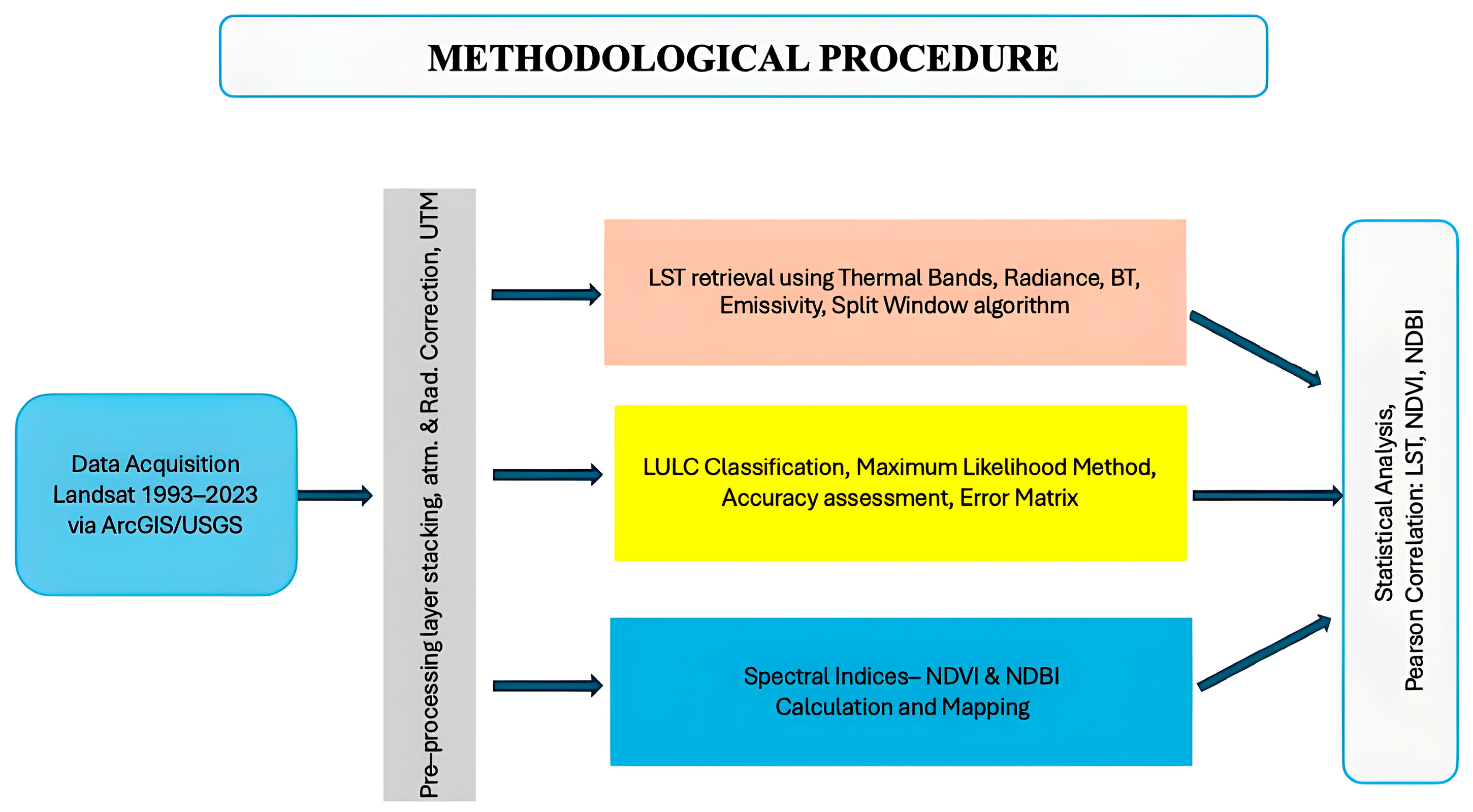
ArcGIS 10.8 was used for picture classification, change detection, and machine learning methods. Land cover and land use changes, LST variations, and other environmental applications were studied in depth using the software. The LULC and LST changes in 1993, 2003, 2013, and 2023 were compared to NDVI and NDBI to find a pattern. LST was examined in June and December of 1993, 2003, 2013, and 2023 to track seasonal fluctuations and avoid cloud cover, whereas LULC, NDVI, and NDBI were analysed in October. US Geological Survey Earth Explorer archives provided three multispectral Landsat (LS) satellite datasets for this study. Landsat 5 TM data were used for 1993, Landsat 7 ETM for 2003, and Landsat 8 OLI for 2013 and 2023. The USGS repository provided imagery metadata. Figure 2 and

Table 2. Metadata of satellite images used for Land Surface Temperature (LST) and spatial indices.

Source	Acquired Date		Spacecraft ID	Cloud Cover		Spatial Resolution	Path/Row
	LST	Spatial Indices		LST	Spatial Indices
Landsat 5	30 June 1993	20 October 1993	Landsat 5 TM	1%	0%	30 m	147/40
Landsat 5	7 December 1993		Landsat 5 TM	3%	0%	30 m	147/40
Landsat 7	1 May 2003	24 October 2003	Landsat 7 ETM	0%	3%	30 m	147/40
Landsat 7	11 December 2003		Landsat 7 ETM	6%	3%	30 m	147/40
Landsat 8	21 June 2013	27 October 2013	Landsat 8 OLI TIRS	0.32%	7%	30 m	147/40
Landsat 8	14 December 2013		Landsat 8 OLI TIRS	9%	7%	30 m	147/40
Landsat 9	9 June 2023	15 October 2023	Landsat 9 OLI TIRS	0%	3%	30 m	147/40
Landsat 8	10 December 2023		Landsat 8 OLI TIRS	3%	3%	30 m	147/40
Data Volume: ~1.2 GB/scene (11 bands); velocity: 16-day revisit (8-day w/overlap); format: Level-1 GeoTIFF (USGS EarthExplorer). Source: https://earthexplorer.usgs.gov/ (Accessed on 10 March 2024).

provide photogrammetry details. Multispectral images with a 30 m spatial resolution were used to identify regional land cover characteristics. Reprojecting the datasets using the Universal Transverse Mercator (UTM) coordinate system ensured spatial uniformity between years. Landsat data were chosen over Sentinel-2 for LST retrieval due to multiple advantages. Landsat 8 TIRS has thermal bands for good split-window LST calculations, while Sentinel-2 does not, making LST calculations difficult. Landsat also maintains a 30-year archive from 1993 to 2023 to ensure consistency. The 30 m resolution captures peri-urban heterogeneity (built-up, fields, vegetation, water), critical for zonal LULC–LST analysis; alternatives compromise local-scale temperature detail. Seasonal effects were applied through specific scene selection of summer LST from June data (low monsoon onset, peak heat) and winter LST from December data (stable cold), across all years (1993, 2003, 2013, 2023), ensuring temporal comparability while reducing cloud cover through USGS metadata filtering (<10%). NDVI, NDBI, and LULC were standardised to October (post-monsoon and post-harvest stability). Distinct summer and winter zonal statistics and trends (e.g., summer LST +6 °C against stable winter conditions) expressly accounted for intra-annual variability.

Using the thermal bands of radiometrically and geometrically corrected Earth Observation Data for the years 1993 LS 5, 2003 LS 7, and 2013 and 2023 LS 8, LST was obtained using Band 6 from LS 5 and LS 7 and Band 10 from LS 8. The equation provided by USGS [46] was used to determine the spectral radiance for 1993, 2003, 2013, and 2023 using the Landsat satellite images. Since Landsat 8 uses OLI and Thermal Infrared Sensors (TIRSs) and Landsat 7 uses Enhanced Thematic Mapper (ETM), the LST determined by Landsat 8 considers emissivity, vegetation percentage, and NDVI.

2.3. Land Surface Temperature Calculation

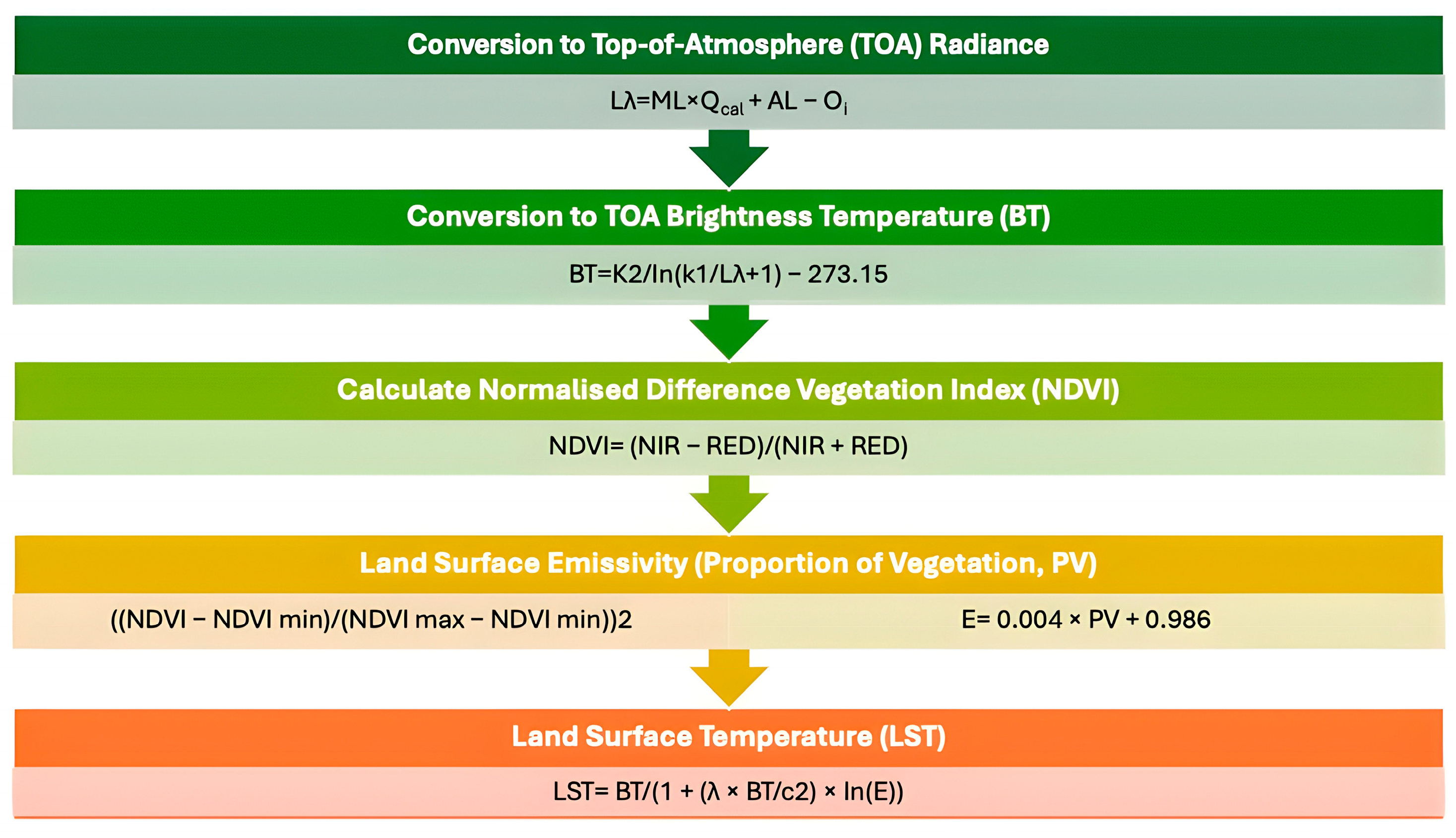
LST was computed using Landsat thermal bands, including LS 5—Band 6, LS 7—Band 6 VCID 2, and LS 8—Band 10, for the years 1993, 2003, 2013, and 2023, using the equations suggested in the available literature [47,48,49]. The administrative boundaries of the study area were delineated using shapefiles in a GIS environment. The split window algorithm (SWA) was used to calculate LST, as provided by USGS (Figure 3) [50].

$$\mathrm{Step} 1: L\lambda =ML\times Qcal+AL-Oi$$

(1)

$$\mathrm{Step} 2: BT=K2/In(k1/L\lambda +1)-273.15$$

(2)

$$\mathrm{Step} 3: NDVI=(NIR-RED)/(NIR+RED)$$

(3)

$$\mathrm{Step} 4: \mathrm{PV}=\left(\right(NDVI-NDVI min)/(NDVI max-NDVI min\left)\right)2$$

(4)

$$\mathrm{Step} 5: E=0.004\times PV+0.986$$

(5)

$$\mathrm{Step} 6: LST=BT/(1+\left(\lambda \times {\displaystyle \frac{BT}{c2}}\right)\times In(E\left)\right)$$

(6)

where Lλ: spectral radiance at top of atmosphere (TOA); ML, A, and 0: coefficients for converting digital number (DN) to TOA radiance; Qcal is quantised DN; BT: brightness temperature; K1, K2: thermal calibration constants; NDVI: Normalised Difference Vegetation Index; Pv: proportion of vegetation; and ε: land surface emissivity (Ref. Figure 3)

2.3.1. Temperature Classification

The calculated LST grid data were reclassified into discrete temperature ranges to identify areas that exceeded average mean temperature thresholds of >20 °C in winter and >35 °C in summer. Pixels within the target temperature ranges were allotted a value of 1, while other pixels were allotted a value of 0. This classification was performed using the Spatial Analyst tool in ArcGIS.

2.3.2. Area Calculation

Each pixel in the raster dataset represents a defined ground area based on the spatial resolution of the dataset. For this study, a resolution of 30 m was used, resulting in an area of 900 m² per pixel. The total area corresponding to pixels within the specified temperature range was calculated using Equation (7) [51]:

$$AREA \left(range\right)=P \left(range\right) \times Area per pixel$$

(7)

where P_range is the total count of pixels classified as 1 and Area per pixel = 900 m² = 0.009 km², as the spatial resolution of satellite images is 30 m (Table 2).

2.4. Land Use/Land Cover (LULC) Classification

The LULC map was classed utilising the Maximum Likelihood Classifier (MLC). The supervised classification approach in ArcGIS 10.8 was preferred for its explicit methodology and high accuracy. MLC evaluates the mean and covariance of each class’s signature prior to assigning a cell to a certain class. Spectral properties were employed to classify the images, which were distinctive for each LS image. Images were categorised using Bands 1–5 and 7 from LS 5 and 7, as well as Bands 1–7 from LS 8. To create LULC maps, all images were initially stacked and processed, utilising the composite band feature of the image processing function. Six overarching LULC categories that may influence LST were examined, predicated on variations in surface radiant temperature. Training samples from six distinct land use types were randomly selected from the image with the help of the Training Sample Manager tool in ArcGIS.

In this study, image classification was validated using an Error Matrix, also referred to as a Confusion Matrix. It is frequently used to explain how well a classification program performs with a collection of test pixels whose true values are known. Accuracy assessment is a crucial stage in image categorisation, evaluating the effectiveness of pixel assignments to appropriate LULC classes. Accuracy is defined as the extent of resemblance between generated and reference maps. Different methodologies and metrics have been developed to evaluate it, which include overall accuracy (OA) and the Kappa coefficient [52]. These metrics indicate the likelihood of accurate classification of randomly chosen locations on a map. To confirm the classified maps, 350 sample points, consisting of six LULC classes, were implicitly gathered from high-resolution Google Earth imagery and used as ground truth points. Each image’s Commission, Omission, Producer’s Accuracy (PA), and User’s Accuracy (UA) were calculated. In addition to the matrix mentioned above, two accepted accuracy assessment coefficients, the Kappa coefficient and overall accuracy (OA), were used.

2.5. Spatial Indices

The NDVI and NDBI remote sensing indices were computed to examine land use changes, urbanisation patterns, and vegetation health in the study area. These indices were derived using LS 5 and LS 8 datasets, acquired for the years 1993, 2003, 2013, and 2023, to visualise a comparative analysis in the past three decades. NDVI (NIR-RED) measures the cooling effects of vegetation (exhibiting a negative correlation with LST), whereas NDBI (SWIR-NIR) identifies heat retention in built environments (showing a positive correlation with LST). Their complementarity is evident as NDVI fails to account for urban impervious surfaces, while NDBI neglects vegetative buffers; collectively, they delineate UHI variance (weak LST-NDVI correlation ~−0.3–0.5; LST-NDBI positive), facilitating targeted interventions in peri-urban areas.

2.5.1. Normalised Difference Vegetation Index (NDVI)

NDVI values vary between +1.0 and −1.0. Areas with barren rock, sand, or snow typically have very low NDVI values (e.g., 0.1 or less). Negative NDVI readings (−1 to about 0) signify the presence of water, ice, and snow. Values near zero signify rock, sand, and dirt; values of 0 to 0.2 denote vegetation, whereas 0.2 to 1 represent thick vegetation, like that found in temperate and tropical forests or crops in their peak growth phase [53]. NDVI was used to evaluate vegetation health and density using Equation (8) [8].

$$NDVI=(NIR-RED)/(NIR+RED)$$

(8)

For LS 5 data, the near-infrared (NIR) (Band 4) and red (Band 3) bands were utilised, while for LS 8, the NIR (Band 5) and red (Band 4) bands were used. The formula was implemented in ArcGIS 10.8 using the Raster Calculator tool.

2.5.2. Normalised Difference Built-Up Index (NDBI)

NDBI was calculated to determine the areas that were urbanised and built-up out of the total area sampled using Equation (9) [54].

$$NDBI=(SWIR-NIR)/(SWIR+NIR)$$

(9)

For LS 5 data, the short-wavelength infrared (SWIR, Band 5) and NIR (Band 4) bands were used, while for LS 8, the SWIR (Band 6) and NIR (Band 5) bands were used. The formula was applied in ArcGIS 10.8 using the Raster Calculator. NDBI values range between −1 and +1, where higher positive values represent built-up areas, while negative values signify vegetation or water bodies. The resulting maps were visualised with a colour gradient to highlight urbanisation patterns.

2.6. Statistical Analysis

Descriptive statistics and correlation analysis were conducted in Microsoft Excel to elucidate the correlation among LST, NDVI, and NDBI. Pearson’s correlation analysis facilitated the study of the dependability among the parameters’ distribution. The Pearson’s correlation coefficient is denoted by Equation (10) [46]

$$r=(\sum (xi-\overline{x}\left)\right(yi-\overline{y}) )/(\surd \sum (xi-\overline{x})2 \sum (yi-\overline{y}\left)2\right),$$

(10)

This study offers a cohesive analytical framework in which LULC provides spatiotemporal context, NDVI and NDBI act as biophysical mediators, and LST measures thermal outcomes. This framework is integrated through zonal statistics (LULC-stratified means of LST, NDVI, and NDBI) and Pearson’s correlations to explain the drivers of UHI effects (contrasting built-up heat with vegetation cooling) across peri-urban gradients, rather than relying on parallel indicators. NDVI alone misses urban impervious surfaces; NDBI overlooks sparse vegetation effects; and LULC alone cannot capture thermal heterogeneity within single classes. Together, via zonal statistics and correlations, they reveal that open fields, despite lower built-up density, exceed cities in LST due to low soil moisture and thermal inertia in semi-arid contexts.

3. Results

3.1. Land Use/Land Cover (LULC) Changes

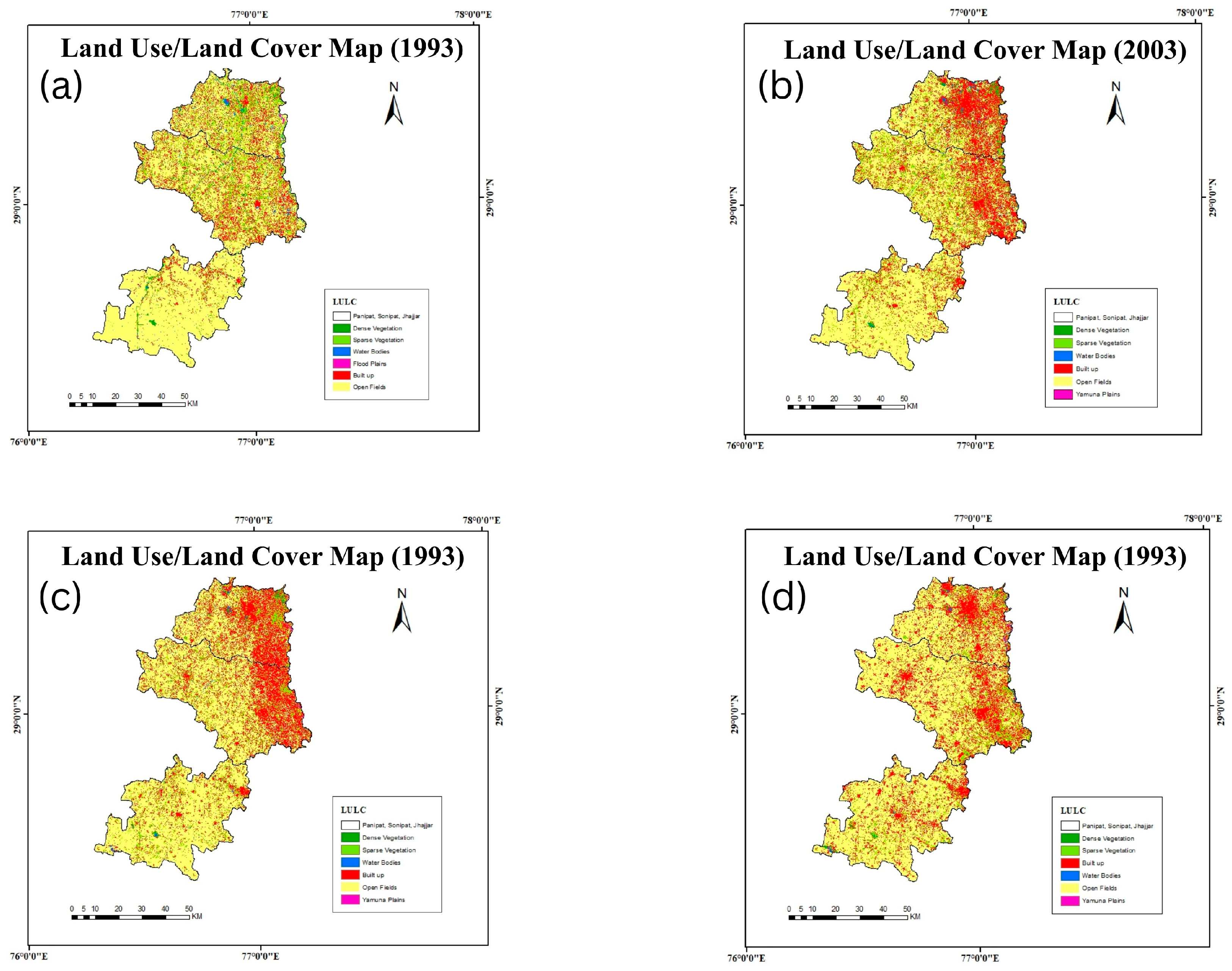
This study shows a significant shift in the land cover of CCF districts from 1993 to 2023, reflecting the impacts of urbanisation and agricultural expansion (Table 3 and Figure 4). Dense vegetation, which encompassed 178.47 km² (3.34%) in 1993, experienced a significant reduction, diminishing to merely 20.66 km² (0.38%) by 2023, highlighting the deforestation and urban expansion that occurred in the region. In 1993, open fields and agricultural lands were the predominant land cover category, encompassing 3475.90 km² (65.13%) in 1993. This category, however, underwent a steady decline, diminishing to 2487.66 km² (46.61%) by 2023 (Table 3). Built-up regions exhibited the most significant growth, increasing from 778.40 km² (14.58%) in 1993 to 2051.07 km² (38.43%) in 2023.

Water bodies saw a significant decline, diminishing from 98.68 km² (1.85%) in 1993 to 33.83 km² (0.63%) in 2023, suggesting potential shrinkage attributable to anthropogenic activity, climatic variations, or urban encroachment (Table 3). The significant alignment of ground truth points with the LULC classification is shown by a Kappa coefficient value of >0.70. The Kappa coefficient values were found to be 0.95, 0.87, 0.80 and 0.73 for 2023, 2013, 2003, and 1993, respectively (Table 3).

Figure 4. Land Use/Land Cover (LULC) change in the CCF region over the 30-year span: (a) 1993, (b) 2003, (c) 2013, and (d) 2023.

Figure 4. Land Use/Land Cover (LULC) change in the CCF region over the 30-year span: (a) 1993, (b) 2003, (c) 2013, and (d) 2023.

Table 3. Decadal changes in Land Use/Land Cover (LULC) area distribution (1993, 2003, 2013, and 2023) and accuracy assessment.

Land Cover	Area 1993		Area 2003		Area 2013		Area 2023
	km2	%	km2	%	km2	%	km2	%
Dense Vegetation	178.47	3.34	159.35	2.99	81.99	1.54	20.66	0.38
Sparse Vegetation	799.65	14.98	821.66	15.4	720.39	13.50	740.28	13.87
Open Fields/Agricultural Land	3475.90	65.13	3018.12	56.55	3119.05	58.44	2487.66	46.61
Built-up	778.40	14.58	1264.34	23.69	1350.81	25.31	2051.07	38.43
Water Bodies	98.68	1.85	71.02	1.33	55.38	1.04	33.83	0.63
Kappa Value	0.73		0.77		0.87		0.95
Overall Accuracy	0.78		0.83		0.89		0.96

Table 3. Decadal changes in Land Use/Land Cover (LULC) area distribution (1993, 2003, 2013, and 2023) and accuracy assessment.

Land Cover	Area 1993		Area 2003		Area 2013		Area 2023
	km2	%	km2	%	km2	%	km2	%
Dense Vegetation	178.47	3.34	159.35	2.99	81.99	1.54	20.66	0.38
Sparse Vegetation	799.65	14.98	821.66	15.4	720.39	13.50	740.28	13.87
Open Fields/Agricultural Land	3475.90	65.13	3018.12	56.55	3119.05	58.44	2487.66	46.61
Built-up	778.40	14.58	1264.34	23.69	1350.81	25.31	2051.07	38.43
Water Bodies	98.68	1.85	71.02	1.33	55.38	1.04	33.83	0.63
Kappa Value	0.73		0.77		0.87		0.95
Overall Accuracy	0.78		0.83		0.89		0.96

3.2. Land Surface Temperature (LST)

3.2.1. Seasonal LST Variation

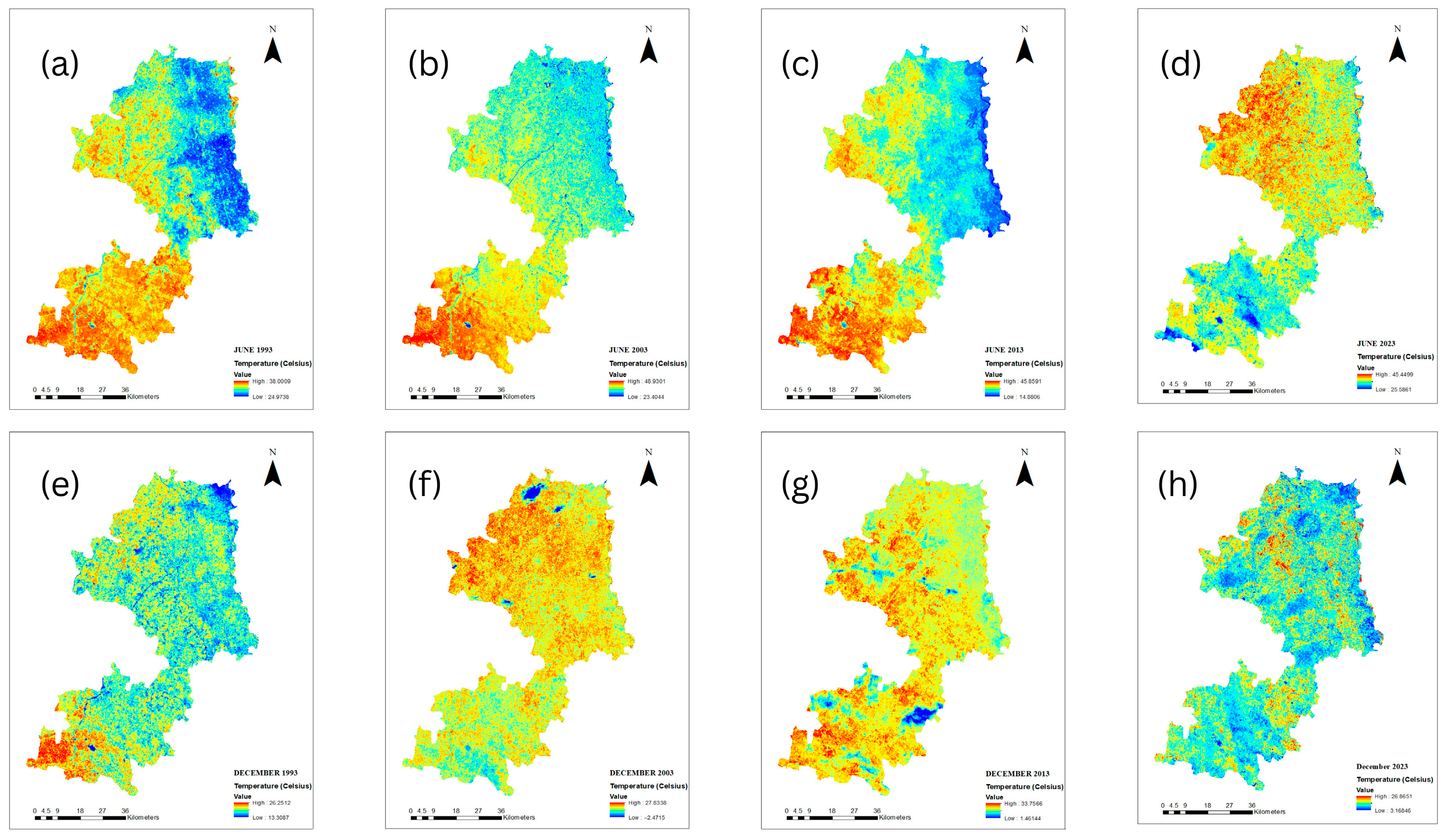
In this study, summer temperatures displayed a consistent upward trend, with the average temperature escalating from 31.43 °C in 1993 to 37.48 °C in 2023 (Table 4). Conversely, winter temperatures exhibited relative stability, with a minor fluctuation from 19.73 °C in 1993 to 19.19 °C in 2023. However, the coefficient of variation indicated a decrease from 11.20% in 2013 to 5.73% in 2023. This implied that winter temperatures in 2023 exhibited less variability compared to 2013. Figure 5 presents the LST for the summer and winter seasons spanning the years 1993, 2003, 2013, and 2023. The data indicate the maximum and minimum LST ranges for each season, expressed in degrees Celsius.

Figure 5. Land Surface Temperature (LST) for the months of June (a) 1993, (b) 2003, (c) 2013, and (d) 2023 and December (e) 1993, (f) 2003, (g) 2013, and (h) 2023.

Figure 5. Land Surface Temperature (LST) for the months of June (a) 1993, (b) 2003, (c) 2013, and (d) 2023 and December (e) 1993, (f) 2003, (g) 2013, and (h) 2023.

Table 4. Descriptive statistics of LST (summer and winter seasons), Normalised Difference Vegetation Index (NDVI), and Normalised Difference Built-up Index (NDBI).

Parameter	LST								NDVI				NDBI
	Summer				Winter
Year	1993	2003	2013	2023	1993	2003	2013	2023	1993	2003	2013	2023	1993	2003	2013	2023
Mean	31.43	35.58	36.07	37.48	19.73	19.26	19.20	19.19	−0.01	−0.01	−0.03	−0.08	−0.01	−0.01	−0.03	−0.08
Min.	24.97	23.40	14.88	25.65	13.30	−2.47	1.46	3.16	−0.35	−0.30	−0.34	−0.31	−0.34	−0.28	−0.32	−0.30
Max.	38.00	48.93	45.74	45.35	26.25	27.83	33.76	26.86	0.36	0.27	0.26	0.31	0.31	0.18	0.24	0.26
Range	13.03	25.53	30.86	19.70	12.94	30.30	32.30	23.70	0.71	0.57	0.60	0.62	0.71	0.57	0.60	0.62
St. Dev.	2.41	2.64	3.92	2.57	1.54	1.46	2.15	1.10	0.08	0.06	0.06	0.08	0.08	0.06	0.06	0.08
Coefficient of Variation (CV)	7.67	7.42	10.87	6.86	7.81	7.58	11.20	5.73	NA

Table 4. Descriptive statistics of LST (summer and winter seasons), Normalised Difference Vegetation Index (NDVI), and Normalised Difference Built-up Index (NDBI).

Parameter	LST								NDVI				NDBI
	Summer				Winter
Year	1993	2003	2013	2023	1993	2003	2013	2023	1993	2003	2013	2023	1993	2003	2013	2023
Mean	31.43	35.58	36.07	37.48	19.73	19.26	19.20	19.19	−0.01	−0.01	−0.03	−0.08	−0.01	−0.01	−0.03	−0.08
Min.	24.97	23.40	14.88	25.65	13.30	−2.47	1.46	3.16	−0.35	−0.30	−0.34	−0.31	−0.34	−0.28	−0.32	−0.30
Max.	38.00	48.93	45.74	45.35	26.25	27.83	33.76	26.86	0.36	0.27	0.26	0.31	0.31	0.18	0.24	0.26
Range	13.03	25.53	30.86	19.70	12.94	30.30	32.30	23.70	0.71	0.57	0.60	0.62	0.71	0.57	0.60	0.62
St. Dev.	2.41	2.64	3.92	2.57	1.54	1.46	2.15	1.10	0.08	0.06	0.06	0.08	0.08	0.06	0.06	0.08
Coefficient of Variation (CV)	7.67	7.42	10.87	6.86	7.81	7.58	11.20	5.73	NA

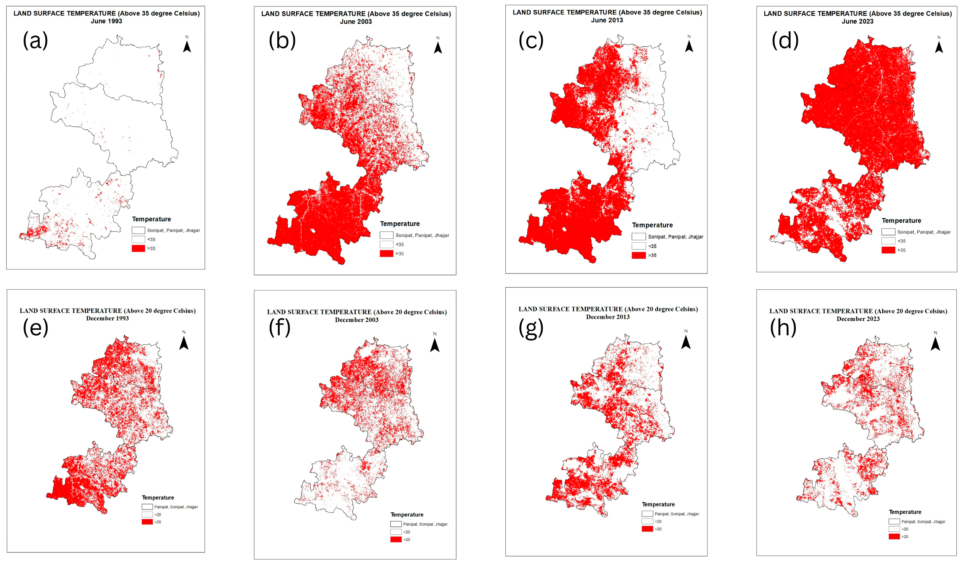
In this study, the CV for summer temperatures decreased from 7.67% in 1993 to 6.86% in 2023, indicating a declining trend of relative variability in summer temperatures, in proportion to the mean temperature during the thirty-year period, despite the increase in temperatures. The coefficient of variation for winter temperatures increased from 7.81% in 1993 to a maximum of 11.20% in 2013, before declining sharply to 5.73% in 2023 (Table 4). In December’s LST data, the percentage of the study area with LST above 20 °C was 45.77% in 1993, but in 2003, it had decreased to 26.91%. Areas with similar temperature coverage decreased to 22.73% in 2023 after increasing to 34.38% in 2013. Summer LST trends, however, showed a dramatic increase in the percentage of the study area with temperatures above 35 °C (average seasonal temperature for this area), especially in recent decades. In 1993, only 2.15% of the total area recorded an LST value above 35 °C, indicating relatively cooler summers in terms of surface temperatures. However, in 2003, this percentage increased to 55.97%; it further increased to 58.64% in 2013 and a remarkable 83.45% in 2023. This dramatic increase in the percentage of area during summer LST could be due to several factors, including the significant increase in built-up areas and UHI effects, coupled with reduced vegetation cover (Figure 6).

3.2.2. Zonal Statistics of LULC and LST

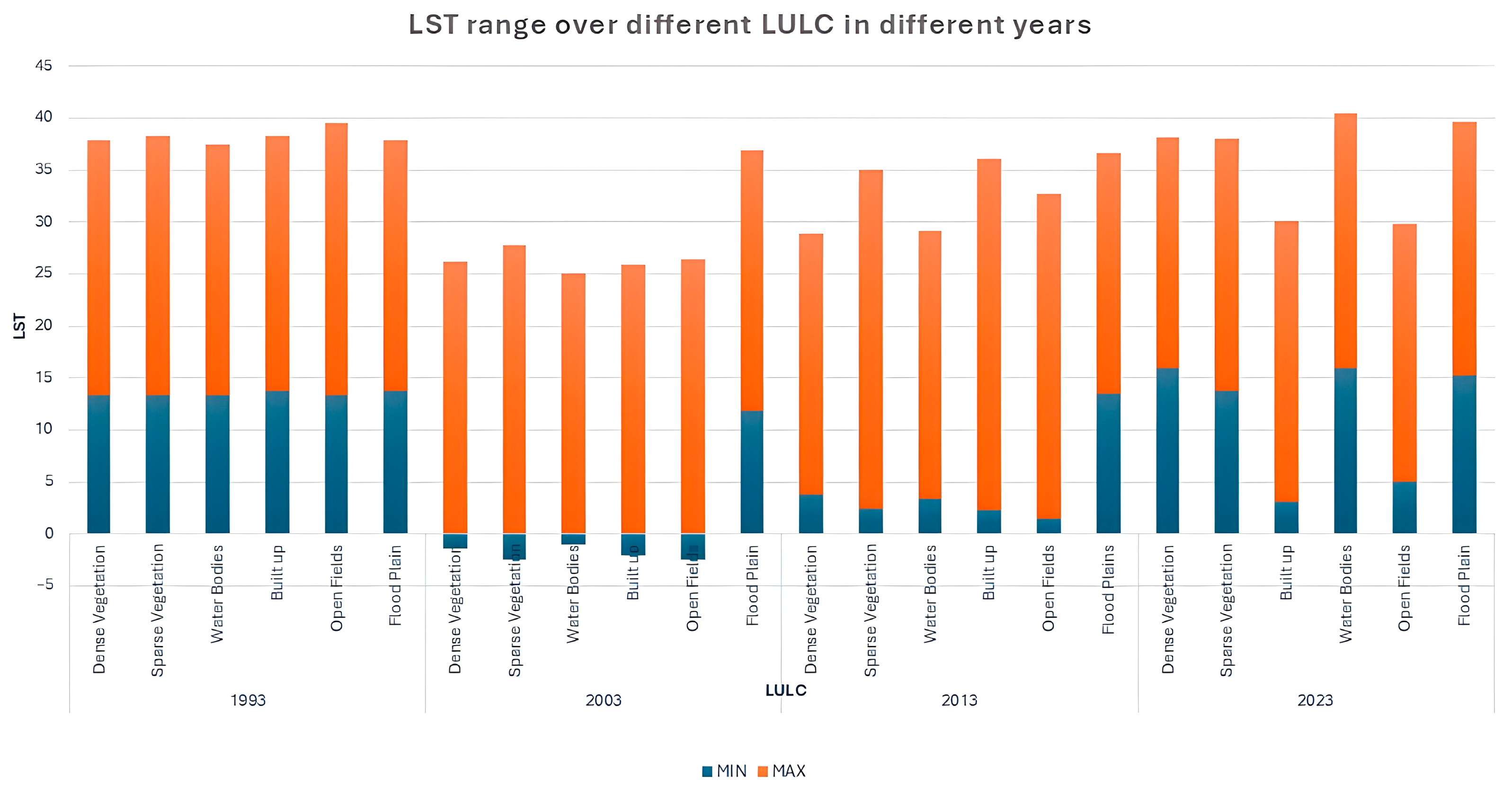
Zonal statistics data from 1993 to 2023 indicated substantial spatial and thermal alterations in the studied region. Figure 7 highlights that in 1993, sparse vegetation and open fields occupied the most extensive areas, with open fields experiencing the maximum LST range of 26.25 °C due to negative NDVI values over these areas, while dense vegetation had the lowest mean LST of 18.17 °C, highlighting its cooling effect. In 2003, open fields also experienced a maximum LST range of 28.94 °C, indicative of heightened thermal stress. In 2013, there was a significant expansion in built-up area, and an LST of 33.76 °C was observed, signifying a heightened UHI effect. Simultaneously, open fields maintained dominance but had a lower mean LST relative to 2003. By 2023, built-up space had grown further, exhibiting thermal fluctuations indicative of continued urbanisation effects, whilst open fields displayed a diminished thermal range (19.65 °C), suggesting possible mitigating measures or vegetation recovery. The temporal examination of the confusion matrices revealed a steady enhancement in classification accuracy, with overall accuracy increasing from 83% in 1993 to 96% in 2023, and the Kappa coefficient rising from 0.77 to 0.95 (Table 3), indicating progress in classification methodologies and data integrity. These findings highlight the substantial influence not only of urbanisation but also of open fields/agricultural land on thermal dynamics and land utilisation patterns in a semi-arid zone. The UHI phenomenon is reflected in the rising LST values for both settlements as well as open fields, highlighting the necessity for sustainable urban planning and afforestation efforts.

3.3. Spatial Indices

3.3.1. Normalised Difference Vegetation Index (NDVI)

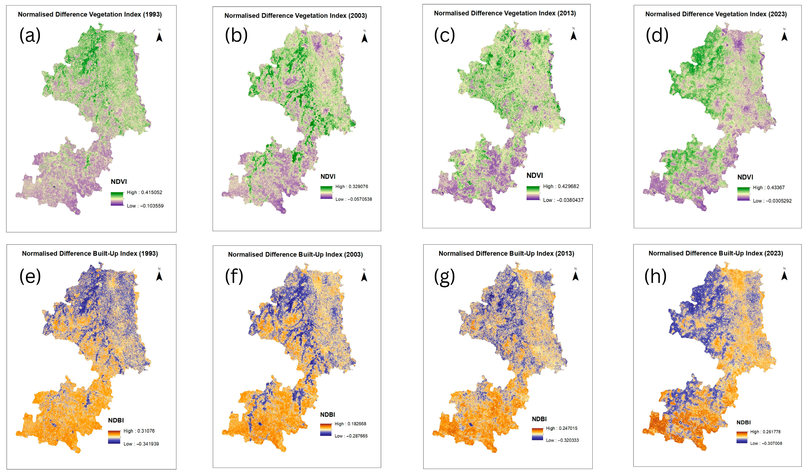
In the present study, the NDVI values remained low, showing a consistent lack of vegetation throughout the study period. The maximum NDVI decreased from 0.36 in 1993 to 0.26 in 2013 but slightly rebounded to 0.31 in 2023 (Table 4 and Figure 8). The negative values indicate either scant or no vegetation, implying a barren region or one with minimal vegetative growth.

3.3.2. Normalised Difference Built-Up Index (NDBI)

In this study, NDBI showed an increase in built-up intensity over time, with a value of −0.34 in 1993, signifying places with negligible built-up intensity, such as vegetation or water bodies (Table 3 and Figure 8). By 2003, the lowest NDBI value marginally improved to −0.28, indicating a reduction in regions with extremely low built-up intensity, while the highest NDBI value decreased to 0.18, reflecting a significant loss in the intensity of built-up areas. This trend persisted into 2013, with the lowest NDBI value of −0.32 and a maximum of 0.24, indicating a minor rebound in built-up intensity relative to 2003, albeit still below the levels of 1993. In 2023, the minimum NDBI value improved to −0.30, and the maximum NDBI value grew slightly to 0.26, indicating a stabilisation or minor revival in built-up intensity relative to the preceding decade.

3.4. Correlation Between LST, NDVI, and NDBI

The analysis of the correlation between LST and NDVI over the years shows varying degrees of relationship. The data reflect significant correlations over the years, with significant variations influenced by the climatic zone of this area. A weak relationship was observed in the study area, as indicated by low R-squared values (

Table 5. Correlation, R-squared, and P-values for the relationships between LST (Land Surface Temperature), NDVI (Normalised Difference Vegetation Index), and NDBI (Normalised Difference Built-up Index) across different years (1993, 2003, 2013, and 2023).

Year	Correlation LST-NDVI	R-Squared LST-NDVI	P-Value LST-NDVI	Correlation LST-NDBI	R-Squared LST-NDBI	P-Value LST-NDBI
1993	−0.46	0.21	0.12	0.47	0.22	0.11
2003	0.50	0.25	0.09	−0.58	0.34	0.04
2013	0.33	0.11	0.28	−0.32	0.10	0.29
2023	0.38	0.14	0.22	−0.35	0.12	0.25

), which are due to the semi-arid climatic conditions of the study area. There was a gradual decline in vegetation’s cooling effect (Figure 7) due to a constant decrease in dense vegetation in the study area (Table 3), especially in open fields. The spatial heterogeneity in correlation values reflects the differential impacts of land use change.

The positive correlation between LST and NDBI indicates that built-up areas contribute to increased surface temperatures. The observations highlight that despite an evident increase in built-up spaces (Table 3), it exhibited negative correlation with rising LST in the region. This can be explained as follows: barren land or open fields reflect high LST due to the lower moisture-retaining capacity in semi-arid climatic conditions, which, in turn, reduces the vegetation health in the area (Table 3). The weak correlations (LST-NDVI r ≈ −0.3 to −0.5; LST-NDBI r ≈ +0.2 to +0.4) indicate non-linear, context-specific urban heat island dynamics in CCF’s semi-arid peri-urban environment, where sparse vegetation (NDVI consistently negative: −0.01 to −0.08) results in negligible cooling, and open agricultural fields (46.61% area) disproportionately elevate LST due to low moisture and thermal inertia. This does not establish causality but highlights spatial mediation—urban expansion intensifies baseline heat from bare soils, with vegetation buffers ineffective due to aridity.

4. Discussion

The study of variations in temperature provides crucial insights into a geographical region’s potential for carbon sequestration and its climatic impacts [14]. Extreme summer temperatures may create heat stress for human survival, as the Wet Bulb Globe Temperature for an occupational environment is 30 °C [55]. This heat stress also directly impacts Haryana’s irrigation-dependent agriculture. The results in Table 3 highlight the necessity for sustainable land management policies. The LULC data in this study indicate a distinct trend of diminishing natural vegetation and water bodies, an increase in open fields, and a rapid expansion of built-up regions, aligning with observations by Alam et al. [56] on urban expansion in Hyderabad driven by economic and political forces that caused environmental degradation. Summer temperatures showed a consistent upward trend, like the LST study in western Haryana’s Hisar region, where maximum LST increased by 17 °C from 1991 to 2022. Calculating the coefficient of variation (CV) is crucial in such studies for understanding climate trends, especially for forecasting seasonal conditions or comprehending how regional weather patterns react to global changes [57]. The summer LST coefficient of variation increased from 11.8% to 19.2% over 30 years, showing increased local thermal variations: dense urban areas retained stable low coefficients of variation (7–9%), while extensive agricultural regions showed rising variability (22–28%), suggesting that semi-arid land without vegetation is a major contributor in thermal volatility within peri-urban mosaics. Bare soil exhibits higher LST values than urbanised surfaces, possibly due to factors like heat concentration, sparse vegetation, low humidity, and the aridity of sandy soil, which has lower water retention and thermal inertia compared to clay soil [58]. This is why conserving dense vegetation and plantation initiatives are essential for alleviating heat stress and sustaining ecological equilibrium in this region.

From 1993 to 2023, NDVI in the CCF districts decreased from −0.01 to −0.08, coinciding with a threefold increase in built-up area. Successive policy cycles—NCR Regional Plans, Haryana Sub-Regional and HUDA development plans, and SEZs—enabled swift urban and infrastructure growth without achieving the intended green buffers [28]. Although Haryana’s agroforestry policies since 1991 increased farm tree cover to 3% via poplar and eucalyptus systems, CCF NDVI reduction has shown limited success in peri-urban forest restoration [59]. Monoculture timber species offer restricted ecological advantages relative to native mixed systems, and urban–industrial expansion near the NCR has surpassed plantation initiatives [59]. The Indian State of Forest Report (ISFR) 2023 identified a state forest area increase (+30.88 km²), yet CCF shows significant dense vegetation loss (3.34% to 0.38%), stressing the need for varied, ecologically oriented agroforestry in urban peripheries. The NDVI decline in CCF indicates governance flaws in incorporating ecological protections into development, beyond climatic factors. In rapidly urbanising CCF districts, green infrastructure, such as urban trees, rooftop greenery, and permeable surfaces, can improve rainwater retention, heat–flood resilience, and lower LST by 2–4 °C [22]. However, the minor fluctuations in NDVI values indicate that the terrain has consistently exhibited low vegetation cover over the years during this time, with only slight alterations in the minimum NDVI values. This minor increase might be due to the higher red reflectance potential of Landsat 8 satellites. In the past, it was observed that Landsat 8 and 7 have similar near-infrared reflectance, but Landsat 8 has larger red reflectance, and its NDVI is lower in bare soil areas, potentially detecting lower NDVI for bare soil and higher NDVI for vegetation compared to ETM+ images [60]. Targeted afforestation, riverside water conservation (repairing floodplains, farm ponds, agroforestry belts), can enhance NDVI, mitigate microclimates in the Yamuna floodplain, and sustain semi-arid watersheds amid rising temperatures.

NDBI is usually more effective in areas where the NDVI value exceeds 0 [61], which is lacking in the current study. Previous studies have demonstrated that NDBI effectively detects built-up regions in urban environments characterised by humid climates, such as Colombo, Sri Lanka, and Montreal, Canada [61]. Conversely, NDBI has exhibited subpar performance in delineating built-up regions in the semi-arid cities of Urumqi and Shihezi in western China [62]. As it was clear from LULC built-up data that there were substantial land use changes in this area, the decreasing NDBI trend can also be associated with the late retrieval of the monsoon during these years, as per official government data [63]. For instance, Cyclone Biparjoy caused a late retrieval of monsoon winds from this region in 2023 [63]. During the monsoon, excessive rainfall increases soil moisture, which can alter the reflectance qualities of the surface [64]. Different SWIR and NIR reflectance between wet soil and plants in comparison to dry conditions may affect NDBI estimations. Another reason could be the semi-arid climatic conditions of this area, as Sonipat and Panipat are in the semi-arid zone, whereas Jhajjar is in the arid climatic zone [36].

The LST pattern connects well with, as well as diverges from, South Asian urbanisation trends. Delhi’s severe UHI effect (+5 °C) reflects dense growth, while CCF’s LST increase (83.45% of the area >35 °C in 2023) stems from scattered urban regions in low-NDVI agricultural zones, yielding thermal stress comparable to dense urban centres in semi-arid settings [24,65]. Weak LST–NDVI correlations (r ~ −0.3 to −0.5) in CCF align with Hisar (maximum LST 42.3 °C, 1991–2022) but differ from coastal cities (Mumbai, Chennai), moderated by sea breezes and vegetation, showing non-linear vegetation cooling dependent on climate. The notable NDBI–LST correlation in Gurugram (R² ≈ 0.98) reflects rapid industrial expansion, yet state agroforestry yields monoculture plantations of little ecological value, with ineffective green belts despite NCR policy goals [23]. Rahimi et al. [66] also observed that the interactions between LST and NDVI vary across biomes and climates, with evidence showing that while cohesive vegetation generally cools temperatures, this effect is not universally consistent and can sometimes lead to negative outcomes as well. CCF exemplifies South Asia’s peri-urban growth challenge in arid areas, requiring adapted green infrastructure, integrated agroforestry, regional water policy, and ecologically suitable species for climate resilience. There also exist some limitations, such as Landsat’s 16-day revisit cycle, which may hinder cloud-free views in December–June; the 30 m resolution, which misses peri-urban transitions; Pearson’s correlation linearity in non-linear semi-arid settings; and across-sensor discrepancies (±0.5–1 °C), mitigated by monthly measurements and zonal statistics. The strengths encompass the 30-year duration covering urbanisation policy cycles, validated LULC (Kappa 0.73–0.95), and integrated NDVI–NDBI–LULC–LST analysis for comprehensive thermal pattern review, establishing CCF as a framework for a South Asian climate-resilient strategy. Future studies applying machine learning (Random Forests, neural networks) [67] and Geographical Weighted Regression (GWR) to capture dynamic LST-NDVI-NDBI interactions in dry environments; using MODIS/Sentinel-1/2 for routine thermal monitoring and flood–drought warnings; correlating LST with socio-economic data (population density, income, health) to identify heat vulnerability in peri-urban areas; and modelling policy scenarios, land use, and thermal forecasts for NCR planning amid climate change may be undertaken for in-depth analysis. These approaches support the transition to predictive frameworks for climate-resilient peri-urban habitats in South Asia.

5. Conclusions

This analysis identifies notable patterns, such as the stabilisation of seasonal LST variability and an increasing trend in summer temperatures. Thermal stress was exacerbated by the region’s significant loss of natural vegetation and water bodies. This 30-year spatiotemporal analysis of the CCF region in Haryana shows a distinct rise in temperatures along with rapid land use changes in the NCR-influenced peri-urban area. The LULC data show that the built-up area grew from 14.58% to 38.43%, but dense vegetation decreased, and water bodies shrank, reflecting a continuous loss of biological buffers. In accordance with these shifts, the summer mean LST escalated from 31.43 °C in 1993 to 37.48 °C in 2023, while the percentage of total area experiencing temperature above 35 °C during summer surged dramatically. NDVI declined while NDBI showed an upsurge in impervious surfaces, which suggests that vegetation cooling becomes more and more limited under semi-arid and peri-urban environments and that urbanisation continues to be a major factor in heat expansion.

The results of this study strongly advocate for specific climate-resilient initiatives in Haryana’s peri-urban development: (i) implementing green infrastructure and urban forestry to restore buffer zones of vegetation in high-NDBI areas, (ii) setting up afforestation and agroforestry belts across urban–rural edges to increase atmospheric cooling, and (iii) promoting water conservation and floodplain restoration (such as pond rejuvenation and watershed buffers within the Yamuna River system) to preserve the water table and mitigate heat events. Implementing these actions into regional development plans and NCR sub-regional schemes may reduce future heat stress while conserving current forest and water resources. This study highlights the significance of long-term satellite archives and the increasing importance of remote sensing big-data integration and preprocessing methods for effective climate-risk tracking and decision support, as highlighted in recent research on satellite big-data frameworks and collection channels. Looking ahead, our future research will expand on these findings by focusing on the quantification of above-ground biomass to evaluate the carbon sequestration potential of the CCF region. We will systematically collect detailed tree parameters, such as Diameter at Breast Height (DBH), height, crown density, and species composition, with the aim of contributing actionable data and analytical tools that can guide sustainable land management and climate-adaptive urban development in the rapidly changing CCF region. These findings highlight the urgent need for targeted urban planning to restore vegetation, safeguard water bodies, and promote afforestation, fostering both climate resilience and ecological stability.

References

1. Derdouri, A.; Wang, R.; Murayama, Y.; Osaragi, T. Understanding the links between LULC changes and SUHI in cities: Insights from two-decadal studies (2001–2020). Remote Sens. 2021, 13, 3654. [Google Scholar] [CrossRef]
2. Adeyeri, O.E.; Folorunsho, A.H.; Ayegbusi, K.I.; Bobde, V.; Adeliyi, T.E.; Ndehedehe, C.E.; Akinsanola, A.A. Land surface dynamics and meteorological forcings modulate land surface temperature characteristics. Sustain. Cities Soc. 2024, 101, 105072. [Google Scholar] [CrossRef]
3. Shahfahad, K.B.; Alam, S.M.; Mondal, M.A.; Noorpoor, A.K.; Tiwari, P.; Lata, S. Longitudinal study of land surface temperature (LST) using mono- and split-window algorithms and its relationship with NDVI and NDBI over selected metro cities of India. Arab. J. Geosci. 2020, 13, 1040. [Google Scholar] [CrossRef]
4. Tran, D.X.; Pla, F.; Latorre-Carmona, P.; Myint, S.W.; Caetano, M.; Kieu, H.V. Characterizing the relationship between land use land cover change and land surface temperature. ISPRS J. Photogramm. Remote Sens. 2017, 124, 119–132. [Google Scholar] [CrossRef]
5. Gupta, H.; Kumar, S.; Pandey, R.; Thapliyal, S.; Shaji, A.; Kumar, A. An overview of anthropogenic changes in land use and land cover, with specific attention to climate change and unsustainable agriculture. Int. J. Environ. Clim. Change 2024, 14, 453–460. [Google Scholar] [CrossRef]
6. Parnell, S. Defining a global urban development agenda. World Dev. 2016, 78, 529–540. [Google Scholar] [CrossRef]
7. Vliet, V.J.; Verburg, P.H.; Gradinaru, S.R.; Hersperger, A.M. Beyond the urban-rural dichotomy: Towards a more nuanced analysis of changes in built-up land. Comput. Environ. Urban Syst. 2019, 74, 41–49. [Google Scholar] [CrossRef]
8. Naidu, K.; Chundeli, F.A. Assessing LULC changes and LST through NDVI and NDBI spatial indicators: A case of Bengaluru, India. GeoJournal 2023, 88, 4335–4350. [Google Scholar] [CrossRef]
9. Zhou, X.; Chen, H. Impact of urbanization-related land use land cover changes and urban morphology changes on the urban heat island phenomenon. Sci. Total Environ. 2018, 635, 1467–1476. [Google Scholar] [CrossRef]
10. Lefevre, A.; Malet-Damour, B.; Boyer, H.; Rivière, G. Urban heat island in the tropics: A review of advances, challenges, and future directions. City Environ. Interact. 2025, 28, 100265. [Google Scholar] [CrossRef]
11. Yadav, A.; Singh, J. A study on urban heat island (UHI): Challenges and opportunities for mitigation. Curr. World Environ. 2024, 19, 436–453. [Google Scholar] [CrossRef]
12. Ramachandra, T.V.; Rana, R.S.; Vinay, S.; Aithal, B.H. Urban heat island linkages with the landscape morphology. Sci. Rep. 2025, 15, 24485. [Google Scholar] [CrossRef] [PubMed]
13. Xiao, X.D.; Dong, L.; Yan, H.; Yang, N.; Xiong, Y. The influence of the spatial characteristics of urban green space on the urban heat island effect in Suzhou Industrial Park. Sustain. Cities Soc. 2018, 40, 428–439. [Google Scholar] [CrossRef]
14. Cui, P.; Xv, D.; Tang, J.; Lu, J.; Wu, Y. Assessing the effects of urban green spaces metrics and spatial structure on LST and carbon sinks in Harbin, a cold region city in China. Sustain. Cities Soc. 2024, 113, 105659. [Google Scholar] [CrossRef]
15. Mukherjee, M.; Takara, K. Urban green space as a countermeasure to increasing urban risk and the UGS-3CC resilience framework. Int. J. Disaster Risk Reduct. 2018, 28, 854–861. [Google Scholar] [CrossRef]
16. Grigoraș, G.; Urițescu, B. Land use/land cover changes dynamics and their effects on surface urban heat island in Bucharest, Romania. Int. J. Appl. Earth Obs. Geoinf. 2019, 80, 115–126. [Google Scholar] [CrossRef]
17. Bala, R.; Prasad, R.; Yadav, V.P. Quantification of urban heat intensity with land use/land cover changes using Landsat satellite data over urban landscapes. Theor. Appl. Climatol. 2021, 145, 1–12. [Google Scholar] [CrossRef]
18. Athokpam, V.; Chamroy, T.; Ngairangbam, H. The role of urban green spaces in mitigating climate change: An integrative review of ecological, social, and health benefits. Environ. Rep. 2024, 6, 10–14. [Google Scholar] [CrossRef]
19. Sharma, P.; Yogeswaran, N.; Singh, R. Longitudinal study of urban heat island phenomena in rapidly developing cities: The case of Gurugram. Civ. Eng. Archit. 2025, 13, 2862–2875. [Google Scholar] [CrossRef]
20. Prakash, S.; Norouzi, H. Land surface temperature variability across India: A remote sensing satellite perspective. Theor. Appl. Climatol. 2020, 139, 773–784. [Google Scholar] [CrossRef]
21. Agrawal, Y.; Pandey, H.; Tiwari, P.S. An analytical study of relation between land surface temperature and land use/land cover using spectral indices: A case study of Chandigarh. J. Geomat. 2023, 17, 184–197. [Google Scholar] [CrossRef]
22. Imam, A.U.K.; Banerjee, U.K. Urbanisation and greening of Indian cities: Problems, practices, and policies. Ambio 2016, 45, 442–457. [Google Scholar] [CrossRef] [PubMed]
23. Kumar, P. National Capital Regional Plan 2021: A geographical analysis. Int. J. Res. Eng. IT Soc. Sci. 2021, 9, 189–193. [Google Scholar]
24. Morya, C.P.; Punia, M. Impact of urbanization processes on availability of ecosystem services in National Capital Region of Delhi (1992–2010). Environ. Dev. Sustain. 2022, 24, 7324–7348. [Google Scholar] [CrossRef]
25. Rana, P. A study of territorial expansion of class-I cities of National Capital Region-Haryana. Int. J. Soc. Sci. Interdiscip. Res. 2021, 10, 46–58. [Google Scholar]
26. Teotia, M.K.; Kumar, R. The State of Cities in North-Western India; Centre for Research in Rural and Industrial Development, (CRRID): Chandigarh, India, 2015. [Google Scholar]
27. Kumar, S.; Singh, R. Geospatial applications in land use/land cover change detection for sustainable regional development: The case of central Haryana, India. Geomat. Environ. Eng. 2021, 15, 81–98. [Google Scholar] [CrossRef]
28. Goel, S. Urbanisation and urban systems in Haryana—A geographical perspective. AGPE R. Gondwana Res. Hist. Sci. Econ. Political Soc. Sci. 2022, 3, 24–42. [Google Scholar]
29. Ramaiah, M.; Avtar, R.; Rahman, M.M. Land cover influences on LST in two proposed smart cities of India: Comparative analysis using spectral indices. Land 2020, 9, 292. [Google Scholar] [CrossRef]
30. Kumar, S.; Singh, R. Geospatial approach to analyse the impact of urban development on the urban heat island in Hisar city, Western Haryana, India. Theor. Appl. Climatol. 2025, 156, 141. [Google Scholar] [CrossRef]
31. Sharma, M.; Kumar, S. Spatio-temporal pattern of urbanisation in Haryana: A micro level analysis. Indian J. Soc. Res. 2017, 58, 553. [Google Scholar]
32. Sangwan, H.; Mahima, M. Growth of urban population in Haryana: A spatio-temporal analysis. Int. J. Res. Anal. Rev. 2019, 6, 752–756. [Google Scholar]
33. Singh, J.; Singh, B. Special Economic Zones (SEZs) and regional development in Haryana. Int. Res. J. Commer. Arts Sci. 2014, 5, 384–394. [Google Scholar]
34. Haryana Forest Department. Detail of Forest Nurseries in Central Circle Rohtak. 2023. Available online: https://cdnbbsr.s3waas.gov.in/s3c5866e93cab1776890fe343c9e7063fb/uploads/2023/08/2023080390.pdf (accessed on 3 March 2024).
35. Anurag, A.; Singh, R.; Kumar, S.; Kumar, A.; Singh, D.; Kumar, M.; Singh, S. Changes in weather entities and extreme events in western Haryana, India. J. Agrometeorol. 2018, 20, 135–142. [Google Scholar]
36. Newas, R.; Singh, S.; Singh, D.; Khicher, M.L.; Singh, R. A Textbook on Agricultural Meteorology; CCSHAU, Department of Agricultural Meteorology: Haryana, India, 2006.
37. Singh, R.B. Environmental consequences of agricultural development: A case study from the Green Revolution state of Haryana, India. Agric. Ecosyst. Environ. 2000, 82, 97–103. [Google Scholar] [CrossRef]
38. Yadav, D.B.; Rai, K.N. Perspective and prospects of sustainable agriculture in Haryana. Indian J. Agric. Econ. 2001, 56, 100–115. [Google Scholar]
39. Sharma, M.; Kumar, S. The pattern of urbanization and fluctuations in the urban hierarchy of Haryana, India. In Urban Environment and Smart Cities in Asian Countries; Springer: Cham, Switzerland, 2023; pp. 85–104. [Google Scholar] [CrossRef]
40. Jha, P.; Bansal, T.; Rawat, P.; Kashyap, M.; Yadav, P.K.; Begam, S. Dynamics of urban transformation and regional development: A spatio-temporal analysis of land use change in Panipat City. In Geographical Dimensions of Environmental Sustainability; Springer: Singapore, 2024; pp. 331–353. [Google Scholar] [CrossRef]
41. Haryana Forest Department. List of Block Forests in Haryana State. 2023. Available online: https://cdnbbsr.s3waas.gov.in/s3c5866e93cab1776890fe343c9e7063fb/uploads/2023/08/202308281589428643.pdf (accessed on 15 January 2024).
42. Verma, P.; Jangra, R.; Kaushik, S.P. Geospatial measurement of urban sprawl and land transformation using multi-temporal datasets: A case study of Sonipat-Kundli urban agglomeration. Sustain. Environ. 2024, 10, 2366556. [Google Scholar] [CrossRef]
43. Kumar, V.; Sikarwar, S. Smart concepts for integrated rurban development of historical towns in India: Case of Panipat, Haryana. In From Poverty, Inequality to Smart City: Proceedings of the National Conference on Sustainable Built Environment 2015; Springer: Singapore, 2017; pp. 57–81. [Google Scholar] [CrossRef]
44. Gupta, R.; Misra, A.K.; Sahu, V. Identification of watershed preference management areas under water quality and scarcity constraints: Case of Jhajjar district watershed, India. Appl. Water Sci. 2019, 9, 27. [Google Scholar] [CrossRef]
45. Gupta, R.; Misra, A.K. Groundwater quality analysis of quaternary aquifers in Jhajjar District, Haryana, India: Focus on groundwater fluoride and health implications. Alex. Eng. J. 2018, 57, 375–381. [Google Scholar] [CrossRef]
46. Alademomi, A.S.; Akinkuolie, O.K.; Adebayo, J.O.; Aladesanmi, A.A. The interrelationship between LST, NDVI, NDBI, and land cover change in a section of Lagos metropolis, Nigeria. Appl. Geomat. 2022, 14, 299–314. [Google Scholar] [CrossRef]
47. Das, D.N.; Chakraborti, S.; Saha, G.; Banerjee, A.; Singh, D. Analysing the dynamic relationship of land surface temperature and landuse pattern: A city level analysis of two climatic regions in India. City Environ. Interact. 2020, 8, 100046. [Google Scholar] [CrossRef]
48. Sannigrahi, S.; Pilla, B.; Basu, S.; Basu, B.; Sharma, R.K. Analyzing the role of biophysical compositions in minimizing urban land surface temperature and urban heating. Urban Clim. 2018, 24, 803–819. [Google Scholar] [CrossRef]
49. Dissanayake, D.; Morimoto, T.; Murayama, Y.; Ranagalage, M. Impact of landscape structure on the variation of land surface temperature in sub-Saharan region: A case study of Addis Ababa using Landsat data (1986–2016). Sustainability 2019, 11, 2257. [Google Scholar] [CrossRef]
50. U.S. Geological Survey. Landsat 7 (L7) Data Users Handbook. 2019. Available online: https://d9-wret.s3.us-west-2.amazonaws.com/assets/palladium/production/s3fs-public/media/files/LSDS-1927_Landsat7-Data-Users-Handbook-v3.pdf (accessed on 20 April 2023).
51. ESRI. ArcGIS Pro Zonal Statistics (Spatial Analyst), Tool References. Available online: https://pro.arcgis.com/en/pro-app/latest/tool-reference/spatial-analyst/zonal-statistics.htm (accessed on 7 June 2023).
52. Amini, S.; Saber, M.; Rabiei-Dastjerdi, H.; Homayouni, S. Urban land use and land cover change analysis using random forest classification of Landsat time series. Remote Sens. 2022, 14, 2654. [Google Scholar] [CrossRef]
53. Mansourmoghaddam, M.; Rousta, I.; Ghafarian Malamiri, H.; Sadeghnejad, M.; Krzyszczak, J.; Ferreira, C.S.S. Modeling and estimating the land surface temperature (LST) using remote sensing and machine learning (case study: Yazd, Iran). Remote Sens. 2024, 16, 454. [Google Scholar] [CrossRef]
54. Gessesse, A.A.; Melesse, A.M. Temporal relationships between time series CHIRPS-rainfall estimation and eMODIS-NDVI satellite images in Amhara Region, Ethiopia. In Extreme Hydrology and Climate Variability; Elsevier: Amsterdam, The Netherlands, 2019; pp. 81–92. [Google Scholar] [CrossRef]
55. Bernard, T.E.; Iheanacho, I. Heat index and adjusted temperature as surrogates for wet bulb globe temperature to screen for occupational heat stress. J. Occup. Environ. Hyg. 2015, 12, 323–333. [Google Scholar] [CrossRef]
56. Alam, S.M.; Markandey, K. Consequences of unplanned growth: A case study of metropolitan Hyderabad. In Urban and Regional Planning and Development: 20th Century Forms and 21st Century Transformations; Springer: Cham, Switzerland, 2020; pp. 203–219. [Google Scholar]
57. Paul, S.; Majumder, S.; Ghosh, R. Exploring the LULC dynamics and its relation with land surface temperature variation using split window algorithm: A study of Barasat subdivision, West Bengal, India. Environ. Monit. Assess. 2024, 196, 1070. [Google Scholar] [CrossRef] [PubMed]
58. Azmi, R.; Tekouabou, K.; Diop, E.B.; Chenal, J. Exploring the relationship between urban form and land surface temperature (LST) in a semi-arid region case study of Ben Guerir city-Morocco. Environ. Chall. 2021, 5, 100229. [Google Scholar] [CrossRef]
59. Handa, A.K.; Sirohi, C.; Chavan, S.B.; Dhillon, R.S.; Ahlawat, K.S.; Rizvi, R.H. Agroforestry in Haryana: Status and way forward. Indian J. Agrofor. 2020, 22, 1–10. [Google Scholar]
60. Bogrekci, I.; Lee, W.S. The effects of soil moisture content on reflectance spectra of soils using UV-VIS-NIR spectroscopy. In Proceedings of the 7th International Conference on Precision Agriculture, Minneapolis, MN, USA, 25–28 July 2004. [Google Scholar]
61. Rasul, A.; Balzter, J.; Smith, C.; Remedios, J. Applying built-up and bare-soil indices from Landsat 8 to cities in dry climates. Land 2018, 7, 81. [Google Scholar] [CrossRef]
62. Qian, J.; Zhou, Q.; Chen, X. Improvement of urban land use and land cover classification approach in arid areas. In Proceedings of SPIE—The International Society for Optical Engineering, Proccedings of the Image and Signal Processing for Remote Sensing XVI, Toulouse, France, 20–22 September 2010; SPIE: Bellingham, WA, USA, 2010; pp. 466–475. [Google Scholar]
63. India Meteorological Department (IMD). 2023 Southwest Monsoon End of Season Report. 2023. Available online: https://internal.imd.gov.in/press_release/20231001_pr_2555.pdf (accessed on 10 August 2025).
64. Lobell, D.B.; Asner, G.P. Moisture effects on soil reflectance. Soil Sci. Soc. Am. J. 2002, 66, 722–727. [Google Scholar] [CrossRef]
65. Patel, S.; Indraganti, M.; Jawarneh, R.N. A comprehensive systematic review: Impact of land use/land cover (LULC) on land surface temperatures (LST) and outdoor thermal comfort. Build. Environ. 2024, 249, 111130. [Google Scholar] [CrossRef]
66. Rahimi, E.; Dong, P.; Jung, C. Global NDVI-LST correlation: Temporal and spatial patterns from 2000 to 2024. Environments 2025, 12, 67. [Google Scholar] [CrossRef]
67. Boudriki Semlali, B.-E.; El Amrani, C. Big data and remote sensing: A new software of ingestion. Int. J. Electr. Comput. Eng. (IJECE) 2021, 11, 1521–1530. [Google Scholar] [CrossRef]
Figure 1. Study area details showing the three key districts of the Central Circle Forest (CCF) region, Haryana, India.
Urbansci 10 00095 g001
Figure 2. Flowchart of the methodological procedure adapted in this study.
Urbansci 10 00095 g002
Figure 3. Land Surface Temperature (LST) calculation using the split window algorithm.
Urbansci 10 00095 g003
Figure 6. CCF regions experiencing temperatures above 20 °C and 35 °C in the months of June, for (a) 1993, (b) 2003, (c) 2013, and (d) 2023, and December, for (e) 1993, (f) 2003, (g) 2013, and (h) 2023.
Urbansci 10 00095 g006
Figure 7. Zonal statistics of minimum and maximum temperature ranges for LULC and LST for the years 1993, 2003, 2013, and 2023.
Urbansci 10 00095 g007
Figure 8. Calculated Normalised Difference Vegetation Index (NDVI), for (a) 1993, (b) 2003, (c) 2013, and (d) 2023, and Normalised Difference Built-up Index (NDBI), for (e) 1993, (f) 2003, (g) 2013, and (h) 2023, over the 30-year span.
Urbansci 10 00095 g008