GAN-MIGA-Driven Building Energy Prediction and Block Layout Optimization: A Case Study in Lanzhou, China

Abstract

With the rapid urbanization in China, building energy consumption has become a critical challenge for sustainable urban development. Conventional simulation methods are computationally intensive and inefficient for large-scale urban layout optimization, highlighting the need for fast and reliable predictive approaches. Existing machine learning models often overlook spatial relationships among buildings and rely heavily on manual feature engineering, which limits their applicability at the urban block scale. To address these limitations, the study proposes a building energy consumption prediction model for urban blocks based on Generative Adversarial Networks (GANs), which preserves spatial information while significantly advancing computational speed. The optimal GAN model is further integrated with a Multi-Island Genetic Algorithm (MIGA) to form a GAN-MIGA optimization framework, which is applied to the layout optimization of a target urban block in Lanzhou. Key findings include: (1) the GAN model achieves an average prediction error of 6.8% compared with conventional energy simulations; (2) the GAN-MIGA framework reduces energy consumption by 48.78% relative to the worst-performing solution and by 22.53% compared with the original block layout; (3) the spatial distribution patterns of energy consumption predicted by the GAN are consistent with those obtained from traditional simulation methods; (4) the regression model derived from GAN-MIGA optimization results achieves an R² value exceeding 0.84; and (5) building layout design strategies are formulated based on key morphological indicators in the regression model. Overall, this study demonstrates the effectiveness of the GAN-based method for urban scale building energy prediction and layout optimization. The proposed GAN-MIGA framework provides practical tools and theoretical support for energy-efficient design, policy formulation, and smart city development, contributing to more sustainable urban energy planning.

1. Introduction

1.1. Background of Study

The rapid urbanization of Chinese cities has substantially improved the quality of life for urban residents. However, this growth has also intensified a range of urban environmental challenges, including the urban heat island effect [1], air pollution [2,3], and rising carbon emissions [4]. Among these challenges, carbon emissions have become a particularly pressing concern, drawing sustained attention from governments worldwide. Numerous studies indicate that HVAC systems (Heating, Ventilation, and Air Conditioning) account for a significant proportion of building-related energy usage and are a major contributor to urban carbon emissions [5]. Consequently, improving the energy performance of HVAC systems has become a central component of sustainable urban development strategies.

Statistical data show that in 2020, residential and commercial buildings accounted for 22% and 8% of global energy consumption, respectively, while contributing 17% and 10% of global CO₂ emissions [6]. Within buildings, HVAC systems dominate energy usage; for example, they account for approximately 39% of total building energy consumption in Australia [7]. These figures highlight the critical role of reducing building energy consumption in mitigating urban environmental challenges while simultaneously enhancing the quality of urban life.

As a fundamental urban unit composed of multiple buildings, the building energy consumption (BEC) of urban blocks has attracted increasing research interest. Mutual shading and spatial interactions among buildings within a block can lead to substantial variations in BEC, even under identical climate conditions. Previous studies have demonstrated that morphological and layout parameters play a decisive role in block-scale energy performance [8]. For instance, urban blocks with different floor area ratios (FARs) or building area ratios (BARs) exhibit distinct energy consumption patterns. However, due to the diversity of morphological indicators and their varying emphases, identifying the most effective indicators correlated with BEC and translating them into design strategies remains challenging. Traditional “design-simulation-redesign” workflows rely on repeated manual adjustments, which are labor-intensive, time-consuming, and inefficient for large-scale or iterative design processes [9].

To improve efficiency, optimization algorithms coupled with parametric modeling have been increasingly applied to urban block design [10,11]. For example, large-scale optimization studies involving thousands of iterations have revealed strong correlations between pedestrian-level wind environments and FAR. Because these optimization processes typically use energy consumption as the objective function, accurate and efficient BEC evaluation is essential to ensure algorithmic performance. Physical-based simulation models are widely used for building energy analysis [12,13]; however, their application at urban scale is constrained by high computational costs, extensive input requirements, and the need for specialized expertise. These limitations create a fundamental conflict between long simulation times and the practical demands of iterative urban design optimization.

In response to these challenges, researchers have increasingly adopted machine learning (ML)-based surrogate models for block-scale energy prediction. Data-driven approaches (black-box models) extract patterns from historical datasets using statistical and ML techniques [14]. Models such as Support Vector Machines (SVMs) [15,16], Artificial Neural Networks (ANNs) [17,18,19], and Recurrent Neural Networks (RNNs) [8,20,21] have demonstrated strong predictive performance. Compared with physical simulation models, ML-based approaches generally require fewer input parameters, reduce data processing complexity, and offer strong adaptability. Nevertheless, model development often still involves complex feature selection [22], model architecture design [23], and hyperparameter tuning [24]. Moreover, the black-box nature of many ML models limits their interpretability.

Crucially, existing ML models struggle to incorporate spatial features such as building location and geometry, limiting prediction accuracy at the urban block scale. Nevertheless, the rise of ML has spurred a revival in physical modeling research. Among these, ANN has become mainstream due to its excellent non-linear fitting capability, with related studies rising from 35 in 2016 to 100 in 2020 [25]. This growth is largely due to the success of Multilayer Perceptrons (MLPs), such as Biswas et al.’s residential electricity prediction (R2 = 0.878) [26] and Nasruddin et al.’s annual energy prediction (R2 = 0.9452) [27]. The application of RNN is also increasing [25], indicating the broad applicability of ML in building energy prediction.

Despite their predictive capabilities, due to their statistical-fitting nature, most existing ML surrogate models struggle to effectively incorporate spatial characteristics such as building geometry and relative location. As a result, these models typically rely on simplified design parameters or morphological indicators that lack explicit spatial representation. This limitation causes ML models to capture global trends in energy consumption while failing to reflect localized spatial variations, which are critical for urban block-scale design and optimization. Consequently, their applicability to spatially sensitive design tasks remain limited.

These challenges highlight an urgent need for artificial intelligence methods that can capture spatial relationships without relying on extensive feature engineering. Such methods would enable the development of refined surrogate models with inherent urban spatial awareness, allowing seamless integration with optimization algorithms for efficient and effective urban block energy optimization.

1.2. Generative Adversarial Networks

With the rapid advancement of artificial intelligence, deep learning algorithms have been widely adopted for tasks involving spatial relationship modeling, particularly in images-based and visual data analysis. Compared with traditional machine learning methods, deep learning models—especially convolutional neural networks (CNNs)—exhibit superior performance in spatial perception and representation. This advantage primarily arises from two characteristics. First, CNNs enable end-to-end automatic feature extraction given sufficient labeled data, they can learn discriminative features directly from raw pixel inputs, eliminating the need for labor-intensive and subjective handcrafted feature engineering. Second, their convolutional architecture employs localized receptive fields that systematically scan across images, allowing the model to capture hierarchical spatial structures and contextual dependencies among pixels.

Despite these advantages, CNNs are inherently designed as feed-forward discriminative models for tasks such as classification or recognition. Their architectural focus on discrimination limits their suitability for generative tasks, including data synthesis and predictive modeling. As result, there has been growing interest in generative deep learning frameworks that are capable of learning underlaying data distributions and producing realistic samples.

Among these frameworks, Generative Adversarial Networks (GANs) have emerged as a powerful paradigm for data generation. GANs consist of two neural networks—a generator (G) and a discriminator (D)—that are trained simultaneously through a min-max adversarial process [28]. The generator attempts to produce realistic synthetic samples from random noise, while the discriminator aims to distinguish between real data and generated samples. Through iterative competition, the generator progressively improves its ability to produce plausible outputs, while the discriminator refines its classification capability, ultimately leading to convergence toward highly realistic generated data.

In recent years, GANs have attracted increasing attention in urban physical environment research due to their strong generative capabilities [29,30,31]. By leveraging fully connected or convolutional architectures, GANs can directly process image-like data representations [32,33,34,35], enabling applications in city-scale environmental simulation and prediction [36]. Typically, the generator adopts a deep convolutional structure that facilitates hierarchical feature learning, capturing both low-level characteristics (e.g., edges and textures) and high-level semantic information (e.g., building forms and spatial layouts) [37,38]. Multi-level feature fusion strategies further help preserve structural integrity during conditional generation or style transformation, while allowing adaptive modulation of spatial attributes.

Although GANs have been applied in various urban environment studies, their use in establishing building energy consumption proxy models at the urban block scale remains limited. This limitation can be attributed primarily to two challenges: (1) the substantial computational effort required to generate large-scale training datasets of block-level energy consumption through physical simulations, and (2) the need for domain expertise to transform energy consumption data into formats compatible with GAN-based learning. Together, these challenges have constrained the practical application of GANs for urban scale building energy prediction and optimization.

1.3. Research Gaps

Despite the growing interest in data-driven building energy prediction and urban layout optimization, three critical gaps remain in the existing literature when these methods are applied at the urban block scale:

• Lack of GAN-based energy prediction at block scale.

To date, GANs have not been applied to urban block energy prediction, largely due to the absence of a robust data transformation methodology. In particular, there is no established approach for converting building energy simulation outputs into image-based representations suitable for GAN training.

2.

Limited use of GANs as surrogate models in optimization.

Although some studies have combined GANs with optimization algorithms for urban form optimization, GANs have typically been used only as layout generators. Their potential role as surrogate models that directly participate in the optimization process—by rapidly predicting energy performance—has not been fully explored.

3.

Insufficient morphological analysis of optimization results.

While some studies evaluate energy performance based on optimal solutions, few conduct systematic morphological analyses of the entire solution set generated during the optimization process. As a result, actionable and generalizable design strategies for urban designers remain underdeveloped.

1.4. Aims and Originality

To address the above research gaps, this study proposes an integrated optimization framework that combines GAN-based building energy prediction with urban block layout design, supported by morphological analysis to inform design strategy.

• This study aims to:
  • Develop a Generative Adversarial Network (GAN)-based surrogate model for predicting building energy consumption at urban block level.
  • Establish a coupled GAN-MIGA framework for energy-efficient urban layout optimization.
  • Construct regression models that link morphological indicators to energy performance and derive corresponding layout design strategies for urban designers.
• The originality of this study lies in the following aspects:
  • Proposing a comprehensive methodology for generating image-based datasets from building energy simulation results, specifically tailored for GAN training.
  • Systematically evaluating the predictive performance of multiple GAN architectures under different scenarios using quantitative performance metrics.
  • Validating the generalization capability of GAN-based models by comparing predicted results with simulation outcomes for unseen urban blocks in Lanzhou.
  • Integrating the GAN surrogate model with a Multi-Island Genetic Algorithm (MIGA) to optimize building layouts with respect to energy consumption.
  • Establishing regression models based on morphological indicators extracted from both superior and inferior solution sets, thereby identifying key design parameters and translating optimized results into practical urban design guidance.

2. Materials and Methods

This study develops an integrated optimization framework for urban block layout design by coupling GAN models with parametric design methods. As shown in Figure 1, the research framework consists of seven sequential phases: (1) collection of building and layout data from selected urban blocks in Lanzhou; (2) development of parametric methods for urban block layout generation; (3) configuration of Multi-Island Genetic Algorithm (MIGA) parameters; (4) training of GAN-based building energy consumption prediction models; (5) validation of the prediction performance of the GAN models; (6) optimization of layout design variables; and (7) derivation of urban layout design strategies based on the optimized solution sets.

2.1. The Parametric Building Layout Generation Method

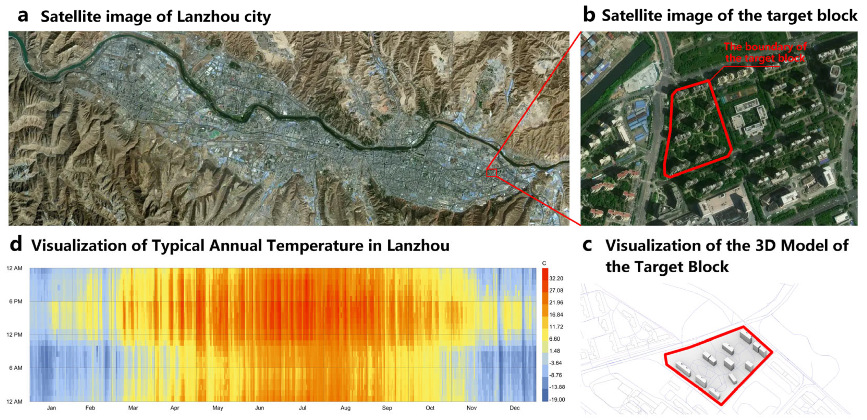
2.1.1. Target Block Selection

As illustrated in Figure 2a, Lanzhou—a representative city located in China’s cold climate region—was selected as the case study. Figure 2d presents local climatic characteristics, with summer temperatures peaking at 32.2 °C and winter temperatures dropping to −19 °C, indicating substantial seasonal thermal variation and significant heating and cooling demands. The selected target block, Xinxinjiayuan East Area in Guancheng District (Figure 2b), exhibits a high-density urban morphology predominantly composed of mid-rise residential buildings. Based on 2020 Baidu Map data (.shp and .dbf files), as shown in Figure 2c, a 3D digital model of the block was reconstructed to accurately represent building geometry and spatial configuration. Quantitative analysis of the block identified a total of 12 residential buildings, with a building area ratio $(\mathrm{B}\mathrm{A}\mathrm{R}$) of 0.12 and a floor area ratio ($\mathrm{F}\mathrm{A}\mathrm{R}$) of 2.2.

2.1.2. Parametric Block Layout Generation Method

Using the existing block layout as a fixed baseline, this study reduces building energy consumption through spatial layout optimization. As shown in Figure 3, twelve buildings are parameterized (${\mathrm{A}}_1$–${\mathrm{A}}_{12}$) within a 37-cell grid system (40 m × 40 m per cell). The centroid of each grid cell represents a potential building location, where the position of each building is defined as ${\mathrm{A}}_{\mathrm{n}}$ ∈ [0, 36]. To ensure the physical feasibility of the generated layouts, two constraints are imposed: (1) when buildings overlap, merge their footprints and adjust the building height accordingly to preserve total volume; (2) the portion of a building footprint that exceeds the boundary is redistributed in block interior, to maintain volumetric consistency. Both constraint mechanisms ensure that all optimized layout solutions remain physically valid and comparable in-built volume.

2.2. The Optimization Settings

2.2.1. The Objective Function

This study focuses on the optimization of annual HVAC energy consumption at the urban block scale. Accordingly, the object function is defined as the total annual building energy consumption (${\mathrm{E}}_{\mathrm{a}\mathrm{l}\mathrm{l}}$), calculated as the annual cooling energy consumption (${\mathrm{E}}_{\mathrm{c}\mathrm{o}\mathrm{o}\mathrm{l}\mathrm{i}\mathrm{n}\mathrm{g}}$) and heating energy consumption (${\mathrm{E}}_{\mathrm{h}\mathrm{e}\mathrm{a}\mathrm{t}\mathrm{i}\mathrm{n}\mathrm{g}}$). The optimization process aims to minimize ${\mathrm{E}}_{\mathrm{a}\mathrm{l}\mathrm{l}}$. Both ${\mathrm{E}}_{\mathrm{c}\mathrm{o}\mathrm{o}\mathrm{l}\mathrm{i}\mathrm{n}\mathrm{g}}$ and ${\mathrm{E}}_{\mathrm{h}\mathrm{e}\mathrm{a}\mathrm{t}\mathrm{i}\mathrm{n}\mathrm{g}}$ are measured in kilowatt-hours (kWh).

$${\mathrm{E}}_{\mathrm{a}\mathrm{l}\mathrm{l}}={\mathrm{E}}_{\mathrm{h}\mathrm{e}\mathrm{a}\mathrm{t}\mathrm{i}\mathrm{n}\mathrm{g}}+{\mathrm{E}}_{\mathrm{c}\mathrm{o}\mathrm{o}\mathrm{l}\mathrm{i}\mathrm{n}\mathrm{g}}$$

(1)

2.2.2. Multiple Island Genetic Algorithm

Because this study addresses a single-objective energy optimization problem, the Multiple Island Genetic Algorithm (MIGA) [39] was adopted instead of multi-objective algorithms (e.g., NSGA-II [40]). As a single-object GA, MIGA enhances global search performance by partitioning the population into multiple sub-populations (islands) that evolve in parallel, with periodic migration of elite individuals between islands. This structure effectively mitigates premature convergence and is particularly advantageous for high-dimensional problems [41]. In addition to conventional GA operators—including selection, crossover, mutation—MIGA incorporates two key mechanisms:

• Pseudo-parallelism: Independent sub-population evolution with scheduled elite migration simulates parallel computing.
• Multi-island model: Isolated GA execution per island preserves diversity through migratory exchange.

2.2.3. Optimization Workflow

Using total block energy consumption (${\mathrm{E}}_{\mathrm{a}\mathrm{l}\mathrm{l}}$) as the objective function, the MIGA-based optimization follows six phases (hyper-parameters in

Table 1. MIGA hyperparameters settings.

Related Parameters	Value	Related Parameters	Value
Sub-population size	10	Elite size	1
Number of Island	5	Rel tournament size	0.5
Number of generations	40	Penalty base	0.0
Rate of crossover	0.9	Penalty multiplier	1000.0
Rate of mutation	0.1	Penalty exponent	2
Rate of migration	0.2	Default variable bound (abs val)	1000.0
Interval of migration	5	Failed Run Penalty Value	1030

):

• Problem definition: configuring 12 independent design variables for building placement with BAR/FAR constraints.
• Multi-island initialization: partitioning population into 5 islands for parallel layout generation and energy evaluation.
• Intra-island operations: 90% genome crossover within islands and 10% mutation.
• Migration: transferring top 2 individuals per island with replacement.
• Objective aggregation: maintaining island-specific evaluation with global elite updating.
• Termination: completing 40 generations (2000 total evaluations).

The entire optimization process was automated using iSight 2023 [42]. The workflow consists of three main steps: (1) generation of GAN input data using Grasshopper, (2) prediction of building energy consumption using Python 3.14.2 scripts, and (3) mapping of predicted energy results back to individual buildings in Grasshopper. These steps are executed sequentially by iSight through batch (.bat) file calls. All MIGA hyperparameters were set based on iSight default recommendations.

Focusing on Lanzhou Xinxin Community East District as a case study, this research integrates urban morphology indicators—building area ratio ($\mathrm{B}\mathrm{A}\mathrm{R}$) and floor area ratio ($\mathrm{F}\mathrm{A}\mathrm{R}$)—as penalty constraints in the optimization process. With original $\mathrm{B}\mathrm{A}\mathrm{R}$ (0.12) and $\mathrm{F}\mathrm{A}\mathrm{R}$ (2.2) as baselines, the constraints are set at $\mathrm{B}\mathrm{A}\mathrm{R}$ ∈ [0.09, 0.13] and $\mathrm{F}\mathrm{A}\mathrm{R}$ ∈ [1.8, 2.5]. A linear penalty mechanism is applied to reduce the fitness value proportionally when candidate solutions exceed these thresholds. This ensures a balance between exploratory search efficiency and compliance with urban design regulations. This dual-constraint approach effectively filters out non-viable solutions during optimization.

2.3. The GAN Energy Predict Model

Generative Adversarial Networks (GANs) accommodate multimodal data, including numerical, textual, audio, and image formats. To explicitly capture inter-building occlusion relationships, this study employs image-based data for GAN training. The workflow involves:

• Converting buildings information of Lanzhou’s Yellow River blocks into “block images”.
• Generating paired “energy images” by encoding energy simulation results (via Grasshopper) into RGB values.
• Training a GAN-based model with image pairs.
• Evaluating model performance through loss values and Fréchet Inception Distance (FID).
• Integrating the trained GAN with Grasshopper to inversely decode RGB values into energy consumption metrics.

2.3.1. Selection of GAN Training Blocks

This study focuses on residential urban blocks along the Yellow River in Lanzhou. Built between 2000 and 2010, these energy-inefficient blocks exhibit high energy consumption due to outdated design (Figure 4). Based on 2020 Baidu Map data, a total of 275 residential blocks were selected (excluding the target block), with 265 (green) for GAN model training and 10 (blue) for validation.

2.3.2. Energy Simulation Setup

This study conducts energy consumption simulations for the 265 selected urban blocks. The simulations are performed using Honeybee [43], a plugin within the Grasshopper parametric platform in Rhino, which facilitates the modeling and analysis of building energy consumption [44]. For each urban block, the study records the annual operational energy consumption of every building in the block, measured in kilowatts hour (kWh). To improve simulation efficiency, the building functions and material properties within each block are standardized. This study will configure building materials, internal loads and lighting densities, occupant densities and schedules, HVAC set-points, and operation schedules according to both national (GBT51161-2016 [45]) and regional (JGJ26-2018 [46]) design standards.

In terms of meteorological data, the study selected the EnergyPlus Weather (EPW) file (CHN_Gansu.Lanzhou.528890_SWERA) for simulation calculations. As shown in Appendix A 

Table A1. Energy simulation settings.

The Setting Name	Value	Unit
Num of people per area	0.028	per/m2
Equipment load per area	6.70	W/m2
Lighting density per area	9.00	W/m2
Infiltration rate per area	0.000569	m3/s per m2
Ventilation per area	0.001	m3/s per m2
Ventilation per person	0.008	m3/s per person
Heating set-point	21	°C
Cooling set-point	24	°C

, the study configured simulation parameters, including the heating set-point and cooling set-point temperatures, which were set according to JGJ26-2018. Appendix A 

Table A2. The wall settings.

	Wall
Material	Stucco	Concrete	Insulation-R10 (XPS)	Gypsum
Roughness	Smooth	Rough	Medium Smooth	Smooth
Thickness (m)	0.025	0.25	0.05	0.012
Conductivity (W/m-K)	0.691	1.31	0.020	0.1599
Density (kg/m3)	1858.0	2240.26	50	784.9
Specific Heat (J/kg-K)	836.8	836.26	1000	829.46
Thermal Absorptance	0.9	0.9	0.9	0.9
Solar Absorptance	0.7	0.7	0.7	0.4
Visible Absorptance	0.92	0.7	0.7	0.4

,

Table A3. The roof settings.

	Roof
Material	Insulation	Concrete	Ceiling Air Gap	Acoustic Tile
Roughness	Medium Rough	Medium Rough	Smooth	Medium Smooth
Thickness (m)	0.05	0.2	0.1	0.02
Conductivity (W/m-K)	0.03	1.95	0.556	0.06
Density (kg/m3)	43.0	2240	1.28	368.0
Specific Heat (J/kg-K)	1210.0	900	1000.0	590.0
Thermal Absorptance	0.9	0.9	0.9	0.9
Solar Absorptance	0.7	0.8	0.7	0.2
Visible Absorptance	0.7	0.8	0.7	0.2

and

Table A4. The floor settings.

	Floor
Material	Insulation-R10 (PUR)	Concrete	Carpet pad (SBR)
Roughness	Medium Smooth	Rough	Medium Smooth
Thickness (m)	0.05	0.20	0.02
Conductivity (W/m-K)	0.020	1.31	0.15
Density (kg/m3)	50	2240.26	600
Specific Heat (J/kg-K)	1000	836.26	1500
Thermal Absorptance	0.9	0.9	0.8
Solar Absorptance	0.7	0.7	0.6
Visible Absorptance	0.7	0.7	0.6

show the material settings for the building’s walls, roofs, and floors. Following JGJ26-2018, the study set the window-to-wall ratio (WWR) is 0.3. For window materials settings, given the focus on pre-2015 residential buildings, the study simulated ordinary glass instead of Low-E glass. However, in accordance with JGJ26-2018, the windows were configured as double-glazed units, with detailed settings provided in Appendix A 

Table A5. The window settings.

	Floor
Material	Clean Float Glass	Air	Clean Glass
Thickness (m)	0.006	0.01	0.006
solar transmittance	0.429	None	0.775
solar reflectance front	0.308	None	0.071
solar reflectance back	0.379	None	0.071
visible transmittance	0.334	None	0.881
visible reflectance front	0.453	None	0.08
visible reflectance back	0.505	None	0.08
infrared transmittance	0.0	None	0.0
emissivity front	0.84	None	0.84
emissive back	0.82	None	0.84
conductivity (W/m-K)	0.899	None	0.899
dirt correction factor	1.0	None	1.0
solar diffusing	No	None	No

. The hourly room occupancy rate, lighting system turn-on rate, and equipment system turn-on rate were calculated based on JGJ26-2018 and weighted by room area proportions. The settings are presented in Appendix A 

Table A6. The hourly room occupancy rate.

Room Type	Area Percentage	Hourly Period
		1	2	3	4	5	6	7	8	9	10	11	12
Bedroom	30%	1.0	1.0	1.0	1.0	1.0	1.0	0.5	0.5	0	0	0	0
Living Room	40%	0	0	0	0	0	0	0.5	0.5	1.0	1.0	1.0	1.0
Kitchen	10%	0	0	0	0	0	0	1.0	0	0	0	0	1.0
Bathroom	10%	0	0	0	0	0	0.5	0.5	0.1	0.1	0.1	0.1	0.1
Auxiliary Room	10%	0	0	0	0	0	0.5	0.5	0.1	0.1	0.1	0.1	0.1
Unified Setting		0.30	0.30	0.30	0.30	0.30	0.40	0.55	0.37	0.42	0.42	0.42	0.52
Room Type	Area Percentage	Hourly Period
		13	14	15	16	17	18	19	20	21	22	23	24
Bedroom	30%	0	0	0	0	0	0	0	0	0.5	1.0	1.0	1.0
Living Room	40%	1.0	1.0	1.0	1.0	1.0	1.0	1.0	1.0	0.5	0	0	0
Kitchen	10%	0	0	0	0	0	1.0	0	0	0	0	0	0
Bathroom	10%	0.1	0.1	0,1	0.1	0.1	0.1	0.1	0.5	0.5	0	0	0
Auxiliary Room	10%	0.1	0.1	0.1	0.1	0.1	0.1	0.1	0.1	0.1	0	0	0
Unified Setting		0.42	0.42	0.42	0.42	0.42	0.52	0.42	0.46	0.41	0.30	0.30	0.30

,

Table A7. The lighting system turns-on rate.

Room Type	Area Percentage	Hourly Period
		1	2	3	4	5	6	7	8	9	10	11	12
Bedroom	30%	0	0	0	0	0	1.0	0.5	0	0	0	0	0
Living Room	40%	0	0	0	0	0	0.5	1.0	0	0	0	0	0
Kitchen	10%	0	0	0	0	0	0	1.0	0	0	0	0	0
Bathroom	10%	0	0	0	0	0	0.5	0.5	0.1	0.1	0.1	0.1	0.1
Auxiliary Room	10%	0	0	0	0	0	0.1	0.1	0.1	0.1	0.1	0.1	0.1
Unified Setting		0.00	0.00	0.00	0.00	0.00	0.56	0.71	0.02	0.02	0.02	0.02	0.02
Room Type	Area Percentage	Hourly Period
		13	14	15	16	17	18	19	20	21	22	23	24
Bedroom	30%	0	0	0	0	0	0	0	0	1.0	1.0	0	0
Living Room	40%	0	0	0	0	0	0	1.0	1.0	0.5	0	0	0
Kitchen	10%	0	0	0	0	0	1.0	0	0	0	0	0	0
Bathroom	10%	0.1	0.1	0,1	0.1	0.1	0.1	0.1	0.5	0.5	0	0	0
Auxiliary Room	10%	0.1	0.1	0.1	0.1	0.1	0.1	0.1	0.1	0.1	0	0	0
Unified Setting		0.02	0.02	0.02	0.02	0.02	0.12	0.42	0.46	0.56	0.30	0.00	0.00

and

Table A8. The equipment system turn-on rate.

Room Type	Area Percentage	Hourly Period
		1	2	3	4	5	6	7	8	9	10	11	12
Bedroom	30%	0	0	0	0	0	0	1.0	1.0	0	0	0	0
Living Room	40%	0	0	0	0	0	0	0.5	1.0	1.0	0.5	0.5	1.0
Kitchen	10%	0	0	0	0	0	0	1.0	0	0	0	0	1.0
Bathroom	10%	0	0	0	0	0	0	0	0	0	0	0	0
Auxiliary Room	10%	0	0	0	0	0	0	0	0	0	0	0	0
Unified Setting		0.00	0.00	0.00	0.00	0.00	0.00	0.60	0.70	0.40	0.20	0.20	0.50
Room Type	Area Percentage	Hourly Period
		13	14	15	16	17	18	19	20	21	22	23	24
Bedroom	30%	0	0	0	0	0	0	0	0	1.0	1.0	0	0
Living Room	40%	1.0	0.5	0.5	0.5	0.5	1.0	1.0	1.0	0.5	0	0	0
Kitchen	10%	0	0	0	0	0	1.0	0	0	0	0	0	0
Bathroom	10%	0	0	0	0	0	0	0	0	0	0	0	0
Auxiliary Room	10%	0	0	0	0	0	0	0	0	0	0	0	0
Unified Setting		0.40	0.20	0.20	0.20	0.20	0.50	0.40	0.40	0.50	0.30	0.00	0.00

.

As shown in Figure 5, to reduce computational costs, the building models were simplified by retaining only the primary envelope components—specifically, the roofs, walls, glazing, and slabs—and by standardizing the floor-to-floor height at 3 m for all buildings within the block. To ensure simulation accuracy, each building was simulated individually. For each simulation, the surrounding buildings located within a 100-m radius were included as contextual geometry. The simulation results for each individual building were subsequently aggregated for analysis.

2.3.3. GAN Image Dataset Preparation

As shown in Figure 6, to enhance GAN training efficiency and reduce model complexity, the study implemented the following image processing techniques:

• Image cropping: standardized block images to 256 × 256 pixels with 1:4 scale mapping (1024 m × 1024 m actual area) to address scale-related training complexity.
• Image annotation: converted 3D models from .shp/.dbf files into grayscale “Block Images” where building heights (3 m–123 m) were linearly mapped to 0–255 grayscale values.
• Energy encoding: quantified energy consumption (64 kWh–1,241,600 kWh) into 4096 RGB color combinations by equal interval division and generated “Consumption image”.
• Rotation augmentation: applied clockwise rotations with counterclockwise reversal to maintain dataset alignment.
• Orientation labeling: added north-arrow markers at image corners to preserve spatial relationships between buildings.

2.3.4. GAN Algorithm Settings

For GAN implementation, this study employs CycleGAN [47] (a conditional GAN variant) for building energy prediction. As shown in Figure 7, unlike Pix2Pix, CycleGAN’s dual-cycle architecture enables unpaired image translation. As shown in Figure 7, the two cycles are: 1. Forward cycle (G→Y, D→X); 2. Added backward cycle (G’→X, D’→Y). This design ensures domain consistency without paired training data. Unlike Pix2pix [38], which requires paired image data, CycleGAN’s ability to process unpaired data makes it highly suitable for urban studies. The diversity and complexity of urban blocks often preclude the acquisition of uniform datasets, thereby limiting Pix2pix’s applicability, but not that of CycleGAN.

As shown in Figure 8, one generator and one discriminator for one cycle in CycleGAN [29]. To ensure the cycle consistency of the forward cycle and backward cycle in CycleGAN, cycle consistency loss has been added.

Finally, identity loss as an extra loss, to reinforce the influence of the overall loss and ensure that the output image color matches the original image color, has been added [48]. The final objective of CycleGAN can be expressed as:

$$\mathrm{L}\mathrm{o}\mathrm{s}\mathrm{s}\left(\mathrm{G},\mathrm{F},{\mathrm{D}}_{\mathrm{X}},{\mathrm{D}}_{\mathrm{Y}}\right)={\mathrm{L}\mathrm{o}\mathrm{s}\mathrm{s}}_{\mathrm{c}\mathrm{G}\mathrm{A}\mathrm{N}}\left(\mathrm{G},{\mathrm{D}}_{\mathrm{Y}},\mathrm{X},\mathrm{Y}\right)+{\mathrm{L}\mathrm{o}\mathrm{s}\mathrm{s}}_{\mathrm{c}\mathrm{G}\mathrm{A}\mathrm{N}}\left(\mathrm{F},{\mathrm{D}}_{\mathrm{X}},\mathrm{Y},\mathrm{X}\right)+{\mathsf{\lambda }}_{\mathrm{c}}\ast {\mathrm{L}\mathrm{o}\mathrm{s}\mathrm{s}}_{\mathrm{c}\mathrm{y}\mathrm{c}}\left(\mathrm{G},\mathrm{F}\right)+{\mathsf{\lambda }}_{\mathrm{i}}\ast {\mathrm{L}\mathrm{o}\mathrm{s}\mathrm{s}}_{\mathrm{i}\mathrm{d}\mathrm{e}\mathrm{n}\mathrm{t}\mathrm{i}\mathrm{t}\mathrm{y}}\left(\mathrm{G},\mathrm{F}\right)$$

(2)

To improve the stability of CycleGAN, CycleGAN stores the newly generated images in the image buffer, and the discriminator will be updated based on the image buffer. The hyper-parameter settings for the GAN are shown in

Table 2. GAN hyperparameter settings.

CycleGAN Hyperparameters	Value	CycleGAN Hyperparameters	Value
Batch Size	1	Learning rate of generator	0.0002
$\mathsf{\lambda }$	10	Learning rate of discriminator	0.0002
${\mathsf{\lambda }}_{\mathrm{i}}$	0.5	Number of steps to decay	40,000
Total number of steps	80,000

.

Given the complexity of the GAN architecture, this study adopted the default hyperparameters and network architecture from Keras. This approach was maintained to accommodate the constraints of our computational setup, which consisted of a single 8 GB NVIDIA GeForce RTX 3070 GPU (Custom PC, Wuhan, China), thereby avoiding extensive experimentation.

2.3.5. GAN Model Evaluation

The study evaluates the performance of the GAN models and the accuracy of the final energy consumption prediction model.

Researchers often use loss values to evaluate training GAN performance. However, these values mainly reflect internal optimization and do not directly indicate the visual quality of generated images. Relying solely on loss can be misleading. Therefore, this study introduces the Fréchet Inception Distance (FID) as an additional metric.

FID [49], a method similar to that of human perception, using the inception v3 model to describe the distribution distances between samples and real images, is employed in quantitative evaluation. The lower the FID score, the higher the similarity between the sample image and the target image. Liu et al. [50] trained a GAN model by the MINIST dataset to generate handwritten images with FID scores ranging from 78.0 to 299.0. Park et al. [51] compared the trained models on four high-resolution pre-labeled datasets, with an FID range from 22.6 to 104.7.

The model incorporates four loss functions to evaluate GAN performance: Height loss [37], Content loss [37], Cycle loss [47], and ID loss [52]. Height loss ensures consistency in feature map depth, while Content loss preserves semantic fidelity. Cycle loss maintains coherence in cross-domain translation, and ID loss guarantees the matching of identity features. This multi-objective framework comprehensively evaluates the depth and content consistency of the generated images.

As shown in

Table 3. Three GAN models settings.

Dataset Name	Dataset A	Dataset B	Dataset C
Dataset Size	3180 Image Pairs	3180 Image Pairs	265 Image Pairs
Rotation	Yes	Yes	NO
Labeling	Yes	No	Yes
GAN Algorithm	CycleGAN	CycleGAN	CycleGAN

, to analyze the impact of data augmentation methods and image labeling on GAN performance, the study made three different image datasets and trained the GAN model using the same algorithm for each dataset.

2.4. The Energy Predicts Model Evaluation

To assess the model’s predictive accuracy, ten urban blocks excluded from the training dataset were selected. Energy consumption predictions were generated using the GAN-based model and recorded for subsequent analysis. Concurrently, energy simulations were performed for the identical blocks, enabling direct comparison between simulated and predicted values. As illustrated in Figure 4, these validation blocks share both regional proximity and morphological similarity with the training samples. The agreement between these two datasets quantitatively validates the model’s prediction accuracy.

2.5. The Optimization Result Analysis

The study constructed two solution sets based on optimization history: (1) the optimal set comprising the top solutions with minimum objective function values, and (2) the worst set containing the solutions with maximum objective function values for comparative analysis. Morphological differences between these sets were quantitatively assessed using multiple indicators.

A comprehensive range of morphological indicators was selected to describe the building forms of the optimal and worst solution sets (

Table 4. Eight selected morphological indicators.

Morphological Indicator	Formula	Unit	Nomenclature	Description
Building Area Ratio	$\mathit{BAR} ={\displaystyle \frac{ {\sum }_{i=1}^n{\mathit{BA}}_i}{\mathit{BSA}}}$	None	$BAR$	${\mathit{BA}}_i$ is the footprint area of the $i$ building. $\mathrm{n}$ is the number of buildings in the block. $\mathit{BSA}$ is the block site area.
Floor Area Ratio	$\mathit{FAR}= {\displaystyle \frac{{\sum }_{i=1}^n{(\mathit{BA}}_i \times \frac{{\mathit{BH}}_i}{\mathit{FH}})}{\mathit{BSA}}}$	None	$FAR$	${\mathit{BH}}_i \mathrm{is}$ the height of the $i$ building. $\mathrm{FH}$ is the floor height of buildings, set at 3 m.
Mean Building Height	$\mathit{BH}= {\displaystyle \frac{{\sum }_{i=1}^n{\mathit{BH}}_i}{N}}$	m	$BH$	${\mathit{BH}}_i \mathrm{is}$ the height of the $i$ building.
Standard Deviation of Building Height	${\mathit{BH}}_{\mathit{sd}} =\sqrt{{\displaystyle \frac{{\sum }_{i=1}^n{({\mathit{BH}}_i - \mathit{BH})}^2}{N}}}$	m	${BH}_{sd}$	$\mathit{BH} \mathrm{is}$ the average height of buildings in the block.
Mean Building-to-Building Distance	$\mathit{BTB}= {\displaystyle \frac{{\sum }_{i=1}^n\mathit{min}{d}_{\mathit{ij}}}{N}}$	m	$BTB$	$\mathit{min}{d}_{\mathit{ij}}$ is the minimum spacing value between a single building and all its adjacent buildings.
Mean Distance of Buildings to Block Center	$\mathit{BTC}= {\displaystyle \frac{{\sum }_{i=1}^n{\mathit{BTC}}_i}{N}}$	m	$BTC$	${\mathit{BTC}}_i$ is the distance from the $i$ building to the block centre.
North–South Projection Facade Ratio	${PFA}_{ns}={\displaystyle \frac{{Area}_{Buildings}^{ns}}{{Area}_{max}^{ns}}}$	None	${PFA}_{ns}$	${Area}_{Buildings}^{ns}$ is the total area of building projection areas in the north-south direction. ${Area}_{max}^{ns}$ is the area of the largest projected rectangle in the north-south direction.
East–West Projection Facade Ratio	${PFA}_{ew}={\displaystyle \frac{{Area}_{Buildings}^{ew}}{{Area}_{max}^{ew}}}$	None	${PFA}_{ew}$	${Area}_{Buildings}^{ew}$ is the total area of building projection areas in the east-west direction. ${Area}_{max}^{ew}$ is the area of the largest projected rectangle in the east-west direction.

). These include $\mathrm{B}\mathrm{A}\mathrm{R}$, $\mathrm{F}\mathrm{A}\mathrm{R}$, $\mathrm{B}\mathrm{H}$, ${\mathrm{B}\mathrm{H}}_{\mathrm{s}\mathrm{d}}$, $\mathrm{B}\mathrm{T}\mathrm{B}$, $\mathrm{B}\mathrm{T}\mathrm{C}$, ${\mathrm{P}\mathrm{F}\mathrm{A}}_{\mathrm{n}\mathrm{s}}$, and ${\mathrm{P}\mathrm{F}\mathrm{A}}_{\mathrm{e}\mathrm{w}}$, which collectively describe the compactness, height, layout, and axial distribution of the blocks. Given that building energy consumption is significantly influenced by mutual shading, these metrics were chosen to characterize the mutual shading in both planar and vertical dimensions. Specifically, $\mathrm{B}\mathrm{A}\mathrm{R}$, $\mathrm{B}\mathrm{T}\mathrm{B}$, and $\mathrm{B}\mathrm{T}\mathrm{C}$ represent planar congestion, whereas $\mathrm{F}\mathrm{A}\mathrm{R}$, $\mathrm{B}\mathrm{H}$, and ${\mathrm{B}\mathrm{H}}_{\mathrm{s}\mathrm{d}}$ indicate vertical shading. ${\mathrm{P}\mathrm{F}\mathrm{A}}_{\mathrm{n}\mathrm{s}}$ and ${\mathrm{P}\mathrm{F}\mathrm{A}}_{\mathrm{e}\mathrm{w}}$ further delineate the shading distribution along the north-south and east-west axes.

The study establishes a regression model using the morphological indicators [53,54] of blocks (including both optimal and worst solutions) together with their corresponding objective function values. By analyzing the regression model, the influence patterns of different morphological indicators on the objective function are examined, and relevant design strategies are summarized. Since the selected morphological indicators exhibit collinearity, the ridge regression algorithm is adopted to construct the model.

Ridge regression [55], an enhanced variant of ordinary least squares (OLSs), incorporates L2 regularization to mitigate multicollinearity issues. This biased estimation method modifies the loss function by adding a proportional penalty term to the squared sum of regression coefficients, thereby constraining their magnitudes. The loss function can be expressed as:

$$\mathrm{L}\mathrm{o}\mathrm{s}\mathrm{s}\left(\mathsf{\beta }\right)={‖\mathrm{y}-\mathrm{X}\mathsf{\beta }‖}^2+\mathsf{\lambda }{‖\mathsf{\beta }‖}^2$$

(3)

where $\mathrm{y}$ denotes the dependent variable (objective value) vector with dimension $\mathrm{n}\times 1$; $\mathrm{X}$ is the independent variable (feature) matrix with dimension $\mathrm{n}\times \mathrm{p}$; and $\mathsf{\beta }$ represents the regression coefficient vector with dimension $\mathrm{p}\times 1$.$\mathsf{\lambda }$ serves as the regularization coefficient, controlling the penalty intensity on the regression coefficients. In this study, the value of $\mathsf{\lambda }$ is determined by using the K-fold cross-validation method.

3. Results

3.1. GAN Model Performance Evaluation

The three separate training cases were executed on an NVIDIA GeForce RTX 3070 GPU (8 GB) (Custom PC, Wuhan, China) with a Tensor-Flow environment and took approximately 8 to 56 h for the different cases. As shown in Figure 9, a comparison of the training logs for the three models reveals the following patterns:

Model A exhibited stable convergence with minimal fluctuation. Its total loss stabilized quickly, while adversarial, cycle, and identity losses remained low, indicating a well-balanced optimization.

In contrast, Model B showed higher oscillation, including a prominent spike near iteration 40,000, suggesting a less smooth training process potentially due to suboptimal hyperparameters. Although the ID Loss remained low, the Cycle loss displayed slightly higher variance.

Model C demonstrated the most severe instability, with significant spikes in total loss during mid-training (e.g., at 45,000 and 60,000 iterations). This is likely indicative of gradient issues or noisy samples. Even the ID Loss showed reduced stability compared to the other model.

As shown in Figure 10, the FID values of the three models were calculated and visualized. The analysis reveals the following trends:

The figure reveals a clear performance hierarchy among the models. Model A achieves the most favorable balance, with the FID converging to 20–30 (despite an initial spike to 130). Its low FID mean (<10) and moderate FID Cov (20–30) indicate superior image quality and diversity compared to the other models.

Model B demonstrates moderate performance. Although it exhibits a spike (to ~80) during training, the FID eventually stabilizes within the 30–40 range. It maintains a low FID mean (<10), ensuring high average quality, and its FID Cov (20–30) suggests better diversity than Model C.

Conversely, Model C suffers from severe deficiencies in both stability and quality. The FID shows large-amplitude oscillations with spikes exceeding 140. Critically, it exhibits a high FID mean (fluctuating between 40 and 60) and a high FID Cov (60–80). This indicates not only poor average image quality but also a severe lack of diversity in the generated samples.

Based on the quantitative analyses, the study selected the Model A checkpoint at 73,000 iterations (with the lowest FID value) as the pre-trained model for energy consumption prediction in urban blocks.

3.2. The GAN Energy Predicts Model Evaluation

The study conducted GAN prediction result verification for 10 Lanzhou blocks (the blue blocks in Figure 4) that were not part of the dataset. Firstly, the study generated block images for each block. Based on these block images, the pre-trained GAN model was used to generate energy consumption images. Finally, the energy consumption images were read and converted into energy consumption prediction values for each building in the block through parametric methods. On the other hand, the study obtained energy consumption simulation values for each building in the 10 blocks through Energy-plus energy simulation.

As demonstrated in Figure 11, the comparative analysis between simulated and predicted energy consumption values yields the following observations:

• The GAN-predicted energy consumption trends exhibit strong alignment with simulation results, confirming the feasibility of GAN-based urban block energy prediction.
• The average discrepancy across ten urban blocks is 6.15%, demonstrating the model’s suitability for block-level energy evaluation.
• Discrepancies exist in individual blocks: four blocks show over-prediction (GAN > simulation), while six exhibit under-prediction (GAN < simulation), indicating potential stability limitations.
• Block 2 achieves the smallest difference (1.1%, 26.1 M vs. 25.8 M kWh), whereas block 10 shows the largest deviation (14.9%, 42.7 M vs. 36.3 M kWh), suggesting variable model performance across blocks.
• Computational efficiency comparison reveals a 16-fold advantage for GAN predictions (43 s/block) over simulations (11.5 min/block), significantly accelerating the research workflow.

The Section 4 will give a comparative analysis between simulated and predicted values for the five blocks exhibiting the highest prediction errors: block 6 (3.49%), block 7 (9.40%), block 8 (11.37%), block 9 (14.41%), and block 10 (14.99%).

3.3. The Optimization Result

The MIGA algorithm produced 2000 solutions over 40 generations, with 1210 feasible solutions retained after applying BAR (0.09–0.13) and FAR (1.8–2.5) constraints. Key findings are summarized:

• Energy Consumption (Figure 12a): the algorithm effectively reduced energy use, with mean consumption decreasing from 4.6614 × 10⁷ kWh (Gen 1) to 2.3878 × 10⁷ kWh (Gen 40), a 48.78% reduction. Energy consumption decreased by 22.53% (from 3.0821 × 10⁷ kWh to 2.3878 × 10⁷ kWh) in the optimal solution compared to the original layout.
• $\mathrm{B}\mathrm{A}\mathrm{R}$ (Figure 12b): $\mathrm{B}\mathrm{A}\mathrm{R}$ initially increased (peaking at 0.1107 in Gen 6), then declined to 0.08727 in Gen 39, converging toward the lower bound of the acceptable range (0.09–0.13).
• $\mathrm{F}\mathrm{A}\mathrm{R}$ (Figure 12c): $\mathrm{F}\mathrm{A}\mathrm{R}$ decreased in early generations, peaked at 2.49663 in Gen 26, and oscillated near the upper limit of the acceptable range (1.8–2.5).

As shown in Figure 13, the 2000 solutions were visualized in a 3D coordinate system: energy (Z-axis), BAR (X-axis), and FAR (Y-axis). Color coding was employed to differentiate solution attributes: (1) green, all generated solutions (Figure 13a); (2) blue, feasible solutions meeting $\mathrm{B}\mathrm{A}\mathrm{R}$ and $\mathrm{F}\mathrm{A}\mathrm{R}$ constraints (Figure 13b); (3) red, 50 lowest-energy feasible solutions (Figure 13c); (4) purple; 50 highest-energy feasible solutions (Figure 13c).

The 50 lowest-energy solutions exhibited a consumption range of 1.8828 × 10⁷–2.4328 × 10⁷ kWh (mean: 2.2131 × 10⁷ kWh), constituting the optimal set for subsequent analysis. In contrast, the 50 highest-energy solutions spanned 4.5224 × 10⁷–6.2280 × 10⁷ kWh (mean: 4.9718 × 10⁷ kWh), Considered as the worst set. These 100 solutions collectively represent 8.26% of the 1210 feasible solutions.

As shown in Figure 14, energy consumption simulations were conducted on the optimal (top 50) and worst (bottom 50) solutions. Comparisons between GAN-predicted and simulated results show consistent trends:

• For optimal solutions, the GAN-predicted mean (2.213082 × 10⁷ kWh) was 14.35% lower than the simulated mean (2.58373 × 10⁷ kWh).
• For the worst solutions, the GAN-predicted mean (4.971844 × 10⁷ kWh) exceeded the simulated mean (4.66325 × 10⁷ kWh) by 6.62%.
• Overall, while discrepancies exist between predictions and simulations, the errors remain acceptable. The GAN model consistently captures optimization trends, demonstrating its effectiveness for block-scale energy consumption optimization.

3.4. The Optimization Solutions Analysis

As shown in Figure 15, the block building forms of the optimal solutions (G-01 to G-04) exhibit a high degree of similarity, whereas those of the worst solutions (B-01 to B-04) are more heterogeneous.

As shown in Figure 16, Pearson and Spearman correlation analyses were performed to assess relationships between morphological indicators and block energy consumption. Results reveal:

• Low correlation indicators: ${\mathrm{P}\mathrm{F}\mathrm{A}}_{\mathrm{n}\mathrm{s}}$,${\mathrm{P}\mathrm{F}\mathrm{A}}_{\mathrm{e}\mathrm{w}}$,$\mathrm{B}\mathrm{T}\mathrm{C}$, and ${\mathrm{B}\mathrm{H}}_{\mathrm{s}\mathrm{d}}$ show weak correlations (absolute coefficients ≤ 0.4).
• Strong correlations: $\mathrm{B}\mathrm{A}\mathrm{R}$ exhibits strong positive correlations (coefficients > 0.6), while $\mathrm{B}\mathrm{T}\mathrm{B}$ demonstrates very strong negative correlations (absolute coefficients > 0.8).
• Moderate correlations: $\mathrm{F}\mathrm{A}\mathrm{R}$ shows moderate positive correlation (coefficients < 0.6), and $\mathrm{B}\mathrm{H}$ shows moderate negative correlation (absolute coefficients ≤ 0.6).

3.5. Design Strategies

Based on the 100 solutions (50 optimal and 50 worst), a regression model was constructed using the morphological indicators and the GAN-predicted energy consumption values. Before regression analysis, the study analyzed the correlation and collinearity between morphological indicators separately.

In terms of correlation, as shown in Figure 17a, strong correlations were observed between certain indicators. Specifically, the study identified a strong positive correlation between $\mathrm{B}\mathrm{A}\mathrm{R}$ and $\mathrm{B}\mathrm{H}$ (with an absolute correlation coefficient of 0.73), as well as a significant correlation between ${\mathrm{B}\mathrm{H}}_{\mathrm{s}\mathrm{d}}$ and ${\mathrm{P}\mathrm{F}\mathrm{A}}_{\mathrm{e}\mathrm{w}}$ (reaching an absolute value of 0.77).

Regarding collinearity, the study conducted VIF tests on morphological indicators. As illustrated in Figure 17b, multiple indicators demonstrated significant collinearity issues. The study found that ${\mathrm{B}\mathrm{H}}_{\mathrm{s}\mathrm{d}}$ showed high collinearity with other indicators (VIF = 9.77), $\mathrm{B}\mathrm{T}\mathrm{B}$ and $\mathrm{B}\mathrm{A}\mathrm{R}$ exhibited moderate collinearity (VIF = 7.45 and 5.0)

High correlation and collinearity among indicators can lead to erroneous overall significance in regression models while reducing predictive accuracy. Additionally, it becomes challenging to distinguish the independent contributions of highly correlated variables, thereby diminishing the interpretability of regression models. Consequently, the study adopted the ridge regression algorithm for analysis. This algorithm addresses variance inflation caused by multicollinearity through L2 regularization (ridge parameter $\mathsf{\lambda }$) to constrain regression coefficient.

To evaluate the relative influence of each morphological indicator on the ridge regression model, both the indicators and energy consumption values were normalized. As shown in Figure 18, the model demonstrates high predictive accuracy, with an R2 value of 0.8711. This result indicates that block energy consumption can be effectively predicted using morphological indicators.

The normalized ridge regression model is expressed as follows:

$$\begin{array}{c}\mathrm{E}\mathrm{n}\mathrm{e}\mathrm{r}\mathrm{g}\mathrm{y}=0.4483+0.5133\ast \mathrm{B}\mathrm{A}\mathrm{R}+0.2173\ast \mathrm{F}\mathrm{A}\mathrm{R}+0.1681\ast \mathrm{B}\mathrm{H}-0.0140\ast {\mathrm{B}\mathrm{H}}_{\mathrm{s}\mathrm{d}}-0.8553\ast \mathrm{B}\mathrm{T}\mathrm{B}\\ + 0.0099\ast \mathrm{B}\mathrm{T}\mathrm{C}+0.1103\ast {\mathrm{P}\mathrm{F}\mathrm{A}}_{\mathrm{n}\mathrm{s}}-0.1049\ast {\mathrm{P}\mathrm{F}\mathrm{A}}_{\mathrm{e}\mathrm{w}}\end{array}$$

(4)

Based on the ridge regression coefficients, a selection of morphological indicators was conducted. Since $\mathrm{B}\mathrm{T}\mathrm{C}$ and ${\mathrm{B}\mathrm{H}}_{\mathrm{s}\mathrm{d}}$ showed limited influence, they were excluded. Furthermore, because the values of $\mathrm{B}\mathrm{A}\mathrm{R}$ and $\mathrm{F}\mathrm{A}\mathrm{R}$ are strictly regulated and cannot be easily adjusted by designers, these two indicators were also removed. As shown in Figure 19, a new ridge regression model was constructed based on the remaining four morphological indicators. The new model achieved R2 of 0.8453, indicating good predictive performance.

The normalized ridge regression model is expressed as:

$$\mathrm{E}\mathrm{n}\mathrm{e}\mathrm{r}\mathrm{g}\mathrm{y}=0.4088+0.2148\ast \mathrm{B}\mathrm{H}-0.8394\ast \mathrm{B}\mathrm{T}\mathrm{B}-0.3763\ast {\mathrm{P}\mathrm{F}\mathrm{A}}_{\mathrm{n}\mathrm{s}}+0.7724\ast {\mathrm{P}\mathrm{F}\mathrm{A}}_{\mathrm{e}\mathrm{w}}$$

(5)

Based on the regression coefficients of these four morphological indicators, the following energy reduction strategies were found:

• Building spacing: the negative correlation of $\mathrm{B}\mathrm{T}\mathrm{B}$ indicates that larger spacing reduces mutual shading, thereby decreasing winter heating demand and overall energy consumption.
• Layout orientation: the positive coefficient of ${\mathrm{P}\mathrm{F}\mathrm{A}}_{\mathrm{e}\mathrm{w}}$ suggests avoiding compact east-west layouts; larger north-south spacing enhances solar access, reducing winter heating demand. The negative coefficient of ${\mathrm{P}\mathrm{F}\mathrm{A}}_{\mathrm{n}\mathrm{s}}$ suggests dispersed north-south layouts to maximize south façade solar exposure.
• Building height: the positive coefficient of $\mathrm{B}\mathrm{H}$ shows that taller buildings exacerbate shading effects. Lower average heights mitigate mutual shading and reduce heating energy consumption.

Given the sensitivity of heating loads to solar irradiation in cold climates, the design strategy focuses on minimizing shading via horizontal layout (east-west spacing and south-facing facades) and height control. Consistent with Ridge Regression results, morphological indicators $\mathrm{B}\mathrm{T}\mathrm{B}$ and ${\mathrm{P}\mathrm{F}\mathrm{A}}_{\mathrm{e}\mathrm{w}}$ were found to be more important on energy use than $\mathrm{B}\mathrm{H}$ and ${\mathrm{P}\mathrm{F}\mathrm{A}}_{\mathrm{n}\mathrm{s}}$, highlighting the primacy of planar configuration.

4. Discussion

4.1. Validation of GAN Energy Prediction Spatial Distribution

The study conducted a comparative analysis of energy prediction spatial distribution data and simulated energy consumption spatial distribution data for 5 validation blocks. As shown in Figure 20, the study found:

• Comparing the GAN prediction image and energy simulation image, the GAN energy prediction spatial distribution for Blocks 6–10 is relatively consistent with the energy simulation spatial distribution, indicating that the accurate spatial distribution characteristics of GAN prediction model.
• The energy consumption prediction errors for blocks 7, 8, and 9 are mainly concentrated in the pink circles. The GAN prediction model overestimates the energy consumption of these buildings. This is mainly because the prediction results of the GAN prediction model rely on the energy data in the training set, when the energy data of small buildings are not included in the dataset, errors will occur in the GAN prediction model’s results.
• In block 10, the energy consumption prediction errors are mainly concentrated in the pink circles. As seen from the block image, the two buildings in the pink circles are highly similar and adjacent. The GAN prediction model will consider these two buildings as one, making it difficult to accurately predict the energy consumption data by GAN model.

4.2. Validation of Design Strategies by Simulation-MIGA method

To verify the rationality of the design strategy based on GAN-MIGA, the study combines building energy simulation with optimization algorithms, conducts optimization calculations for the block by the Simulation-MIGA framework, and establishes a ridge regression model through the optimized solutions.

Using the MIGA algorithm, the simulation-based optimization method generated 2000 solutions after 40 generations. Figure 21 presents the optimization results:

• Energy consumption: as shown in Figure 21a, the MIGA algorithm reduced block energy consumption by 34.42% (from 3.4397 × 10⁷ kWh to 2.5589 × 10⁷ kWh) over 40 generations.
• $\mathrm{B}\mathrm{A}\mathrm{R}$: as shown in Figure 21b, it decreased continuously from 0.1110 (Gen 2) to 0.09202 (Gen 29).
• $\mathrm{F}\mathrm{A}\mathrm{R}$: as shown in Figure 21c, peaked at 2.5347 (Gen 7) and declined to 2.5041 (Gen 40) after initial growth.

Under $\mathrm{B}\mathrm{A}\mathrm{R}$ and $\mathrm{F}\mathrm{A}\mathrm{R}$ constraints, 287 feasible solutions were filtered—only 23.72% of the solutions of GAN-based optimization history. For comparative analysis, 30 solutions (10.45% of total) were selected: 15 lowest-energy (optimal) and 15 highest-energy (worst) cases.

A ridge regression model was established using normalized morphological indicators and energy results from these 30 solutions. The model achieved high predictive accuracy (R² = 0.9601), as illustrated in Figure 22, demonstrating the significant influence of morphological indicators on energy consumption. This result indicates that block energy consumption can be effectively predicted using morphological indicators.

The normalized ridge regression model is expressed as:

$$\mathrm{E}\mathrm{n}\mathrm{e}\mathrm{r}\mathrm{g}\mathrm{y}=-0.1937+0.1874\ast \mathrm{B}\mathrm{H}-0.6579\ast \mathrm{B}\mathrm{T}\mathrm{B}-0.5876\ast {\mathrm{P}\mathrm{F}\mathrm{A}}_{\mathrm{n}\mathrm{s}}+1.5655\ast {\mathrm{P}\mathrm{F}\mathrm{A}}_{\mathrm{e}\mathrm{w}}$$

(6)

The ridge regression models built from GAN-based and simulation-based optimization results were compared, revealing the following key observations:

• Same indicators: both models incorporated $\mathrm{B}\mathrm{T}\mathrm{B}$, ${\mathrm{P}\mathrm{F}\mathrm{A}}_{\mathrm{n}\mathrm{s}}$, ${\mathrm{P}\mathrm{F}\mathrm{A}}_{\mathrm{ew}}$, and $\mathrm{B}\mathrm{H}$ as predictors, demonstrating robust predictive performance.
• Same influence directions: ${\mathrm{P}\mathrm{F}\mathrm{A}}_{\mathrm{ew}}$ and $\mathrm{B}\mathrm{H}$ show positive correlation with models; $\mathrm{B}\mathrm{T}\mathrm{B}$ and ${\mathrm{P}\mathrm{F}\mathrm{A}}_{\mathrm{n}\mathrm{s}}$ show negative correlation with models.

Table 5. The time cost comparison.

Optimization Method	Model Preparation Time	Average Time per Run	Total Number of Runs	Total Time
GAN-based Optimization	30.5 h	1 min 20 s	2000	74.5 h
Simulation-based Optimization	None	6 min 40 s	2000	222 h

presents the time cost of two methods: 1. Single-run computation: The simulation-based method required almost 5 times longer computation time than the GAN-based prediction. 2. Total computation time: The simulation-based approach also consumed 5 times more time overall.

The GAN-based optimization method outperforms the simulation-based approach in computational efficiency. Trained on a large dataset of urban blocks in Lanzhou, the GAN energy prediction model demonstrates strong generalization, enabling rapid simulation for different block layouts. In contrast, the simulation-based method requires extensive runs for each new layout, leading to significant time overhead in large-scale studies—limiting its practicality in real design projects.

5. Conclusions

This study developed a GAN-based optimization framework for urban block building layout design in Lanzhou city, with annual building energy consumption as the primary optimization objective. Taking a residential block in Lanzhou as a case study, building layout design variables were systematically optimized, and block-scale morphological indicators were employed to derive transferable design strategies. To address the inefficiency of conventional optimization workflows that rely on repeated physical simulations, a GAN-based energy prediction model was integrated, enabling rapid evaluation of design alternatives based on predicted energy performance. By correlating morphological indicators with energy results, predictive regression models were established to support practical urban design decision-making. The key findings are as follows:

• GAN model performance: comparative analysis of loss values and FID across three GAN models revealed that data augmentation significantly enhanced model performance. Semantic label preprocessing further improved prediction accuracy.
• GAN model validation: testing on ten out-of-sample blocks demonstrated that the GAN could generate energy images from block images. Parametric conversion yielded predicted energy values with 1–14.9% errors, drastically reducing computational time while maintaining reliability for block-level optimization.
• Morphology indicators: morphological analysis of 100 solutions identified four key predictors: $\mathrm{B}\mathrm{T}\mathrm{B}$, $\mathrm{B}\mathrm{H}$, ${\mathrm{P}\mathrm{F}\mathrm{A}}_{\mathrm{n}\mathrm{s}}$, and ${\mathrm{P}\mathrm{F}\mathrm{A}}_{\mathrm{ew}}$, all significantly influencing block energy consumption.
• Design strategies: according to ridge regression analysis, maintaining larger building spacing, adopting a more dispersed north-south layout, and a more compact east-west layout collectively increase solar energy in winter, reducing heating demand and total energy consumption.
• Energy spatial distribution: the GAN-based energy prediction model can predict energy consumption for individual buildings in a block while maintaining the spatial information. Although there are some differences compared to simulation results, the distribution trend of GAN predictions is consistent with the simulation results.
• Strategy validation: based on solutions generated from independent simulation-based optimization, this study established a validation ridge regression model to evaluate the effectiveness of the design strategy. The results demonstrate that the validation ridge regression model shares a similar regression formulation with the GAN-based ridge regression model, confirming the validity of the design strategy proposed through the GAN-based optimization process.

6. Limitation and Future Research

6.1. Limitation

This study developed a GAN-based energy consumption prediction model for urban residential blocks in Lanzhou and integrated it with a parametric block layout generation method, and a MIGA optimization algorithm to optimize block-level energy performance. Finally, the study screened solutions from the MIGA optimization process, calculated their morphological indicators, and derived design strategies for architects based on a ridge regression model. While the proposed framework demonstrates promising results, several limitations should be acknowledged.

• Insufficient Energy Simulation Detail: lack of building internal layout data limited detailed energy simulation, reducing surrogate model accuracy.
• Absence of Multi-Objective Optimization: no multi-objective optimization was applied to building systems (e.g., cooling, heating, and lighting), weakening conclusion interpretability and specificity.
• Limited Generalizability: model generalizability is constrained by reliance on Lanzhou’s cold-climate simulation data, limiting applicability to other climatic zones.
• Narrow Optimization Scope: the study focuses solely on energy efficiency, neglecting trade-offs with thermal comfort, cost, and landscape design in block layout optimization.

6.2. Future Research

Future research will address these limitations and focus on the following aspects:

• Future work will collect residential building plans from Lanzhou to develop a detailed parametric block model, followed by energy simulations to train a more accurate GAN model.
• Separate GAN models will be developed for cooling, heating, and lighting systems, and integrated with multi-objective optimization to optimize block layout design.
• The optimization framework will be extended by incorporating additional objectives (e.g., construction cost, landscaping expense, and land use efficiency) to enable comprehensive urban layout optimization via GAN-MIGA.
• Various machine learning algorithms will be employed to build regression models, and their performance will be compared to determine the optimal approach.
• The applicability of GAN-MIGA in optimizing urban street canyons for improved outdoor thermal comfort will be explored in future studies.
• Future studies will collect district data from multiple cold-region cities at similar latitudes to construct a larger-scale dataset. This will be used to train a GAN-based model with enhanced generalization capability for block building energy consumption.

References

1. Arnfield, A. Two decades of urban climate research: A review of turbulence, exchanges of energy and water, and the urban heat island. Int. J. Climatol. 2003, 23, 1–26. [Google Scholar] [CrossRef]
2. Hassan, A.M.; Elmokadem, A.A.; Megahed, N.A.; Abo Eleinen, O.M. Urban morphology as a passive strategy in promoting outdoor air quality. J. Build. Eng. 2020, 29, 101204. [Google Scholar] [CrossRef]
3. Fan, M.; Chau, C.K.; Chan, E.H.W.; Jia, J. A decision support tool for evaluating the air quality and wind comfort induced by different opening configurations for buildings in canyons. Sci. Total Environ. 2017, 574, 569–582. [Google Scholar] [CrossRef]
4. Xu, X.; Ou, J.; Liu, P.; Liu, X.; Zhang, H. Investigating the impacts of three-dimensional spatial structures on CO2 emissions at the urban scale. Sci. Total Environ. 2021, 762, 143096. [Google Scholar] [CrossRef]
5. Bichiou, Y.; Krarti, M. Optimization of envelope and HVAC systems selection for residential buildings. Energy Build. 2011, 43, 3373–3382. [Google Scholar] [CrossRef]
6. IEA. Energy Efficiency; Licence: CC BY 4.0; IEA: Paris, France, 2021; Available online: https://www.iea.org/reports/energy-efficiency-2021 (accessed on 1 January 2020).
7. Jia, Y.; Wang, J.; Reza Hosseini, M.; Shou, W.; Wu, P.; Mao, C. Temporal graph attention network for building thermal load prediction. Energy Build. 2024, 321, 113507. [Google Scholar] [CrossRef]
8. Qiao, Q.; Yunusa-Kaltungo, A.; Edwards, R.E. Towards developing a systematic knowledge trend for building energy consumption prediction. J. Build. Eng. 2020, 35, 101967. [Google Scholar] [CrossRef]
9. Vermeulen, T.; Knopf-Lenoir, C.; Villon, P.; Beckers, B. Urban layout optimization framework to maximize direct solar irradiation. Comput. Environ. Urban Syst. 2015, 51, 1–12. [Google Scholar] [CrossRef]
10. Kaseb, Z.; Rahbar, M. Towards CFD-based optimization of urban wind conditions: Comparison of Genetic algorithm, Particle Swarm Optimization, and a hybrid algorithm. Sustain. Cities Soc. 2022, 77, 103565. [Google Scholar] [CrossRef]
11. Du, Y.; Mak, C.M.; Li, Y. A multi-stage optimization of pedestrian level wind environment and thermal comfort with lift-up design in ideal urban canyons. Sustain. Cities Soc. 2019, 46, 101424. [Google Scholar] [CrossRef]
12. Zhou, Y.P.; Wu, J.Y.; Wang, R.Z.; Shiochi, S.; Li, Y.M. Simulation and experimental validation of the variable-refrigerant-volume (VRV) air-conditioning system in EnergyPlus. Energy Build. 2008, 40, 1041–1047. [Google Scholar] [CrossRef]
13. Magnier, L.; Haghighat, F. Multiobjective optimization of building design using TRNSYS simulations, genetic algorithm, and Artificial Neural Network. Build. Environ. 2010, 45, 739–746. [Google Scholar] [CrossRef]
14. Zhu, C.; Tian, W.; Yin, B.; Li, Z.; Shi, J. Uncertainty calibration of building energy models by combining approximate Bayesian computation and machine learning algorithms. Appl. Energy 2020, 268, 115025. [Google Scholar] [CrossRef]
15. Li, Q.; Meng, Q.; Cai, J.; Yoshino, H.; Mochida, A. Applying support vector machine to predict hourly cooling load in the building. Appl. Energy 2009, 86, 2249–2256. [Google Scholar] [CrossRef]
16. Shine, P.; Scully, T.; Upton, J.; Murphy, M.D. Annual electricity consumption prediction and future expansion analysis on dairy farms using a support vector machine. Appl. Energy 2019, 250, 1110–1119. [Google Scholar] [CrossRef]
17. Buratti, C.; Barbanera, M.; Palladino, D. An original tool for checking energy performance and certification of buildings by means of Artificial Neural Networks. Appl. Energy 2014, 120, 125–132. [Google Scholar] [CrossRef]
18. Runge, J.; Zmeureanu, R. Forecasting Energy Use in Buildings Using Artificial Neural Networks: A Review. Energies 2019, 12, 3254. [Google Scholar] [CrossRef]
19. Roman, N.D.; Bre, F.; Fachinotti, V.D.; Lamberts, R. Application and characterization of metamodels based on artificial neural networks for building performance simulation: A systematic review. Energy Build. 2020, 217, 109972. [Google Scholar] [CrossRef]
20. Ahmad, M.W.; Mourshed, M.; Rezgui, Y. Trees vs. Neurons: Comparison between random forest and ANN for high-resolution prediction of building energy consumption. Energy Build. 2017, 147, 77–89. [Google Scholar] [CrossRef]
21. Wei, Y.; Zhang, X.; Shi, Y.; Xia, L.; Pan, S.; Wu, J.; Han, M.; Zhao, X. A review of data-driven approaches for prediction and classification of building energy consumption. Renew. Sustain. Energy Rev. 2018, 82, 1027–1047. [Google Scholar] [CrossRef]
22. Lin, X.; Yu, H.; Wang, M.; Li, C.; Wang, Z.; Tang, Y. Electricity Consumption Forecast of High-Rise Office Buildings Based on the Long Short-Term Memory Method. Energies 2021, 14, 4785. [Google Scholar] [CrossRef]
23. Zhou, Y.; Liu, Y.; Wang, D.; Liu, X. Comparison of machine-learning models for predicting short-term building heating load using operational parameters. Energy Build. 2021, 253, 111505. [Google Scholar] [CrossRef]
24. Zhou, X.; Lin, W.; Kumar, R.; Cui, P.; Ma, Z. A data-driven strategy using long short term memory models and reinforcement learning to predict building electricity consumption. Appl. Energy 2022, 306, 118078. [Google Scholar] [CrossRef]
25. Lu, C.; Li, S.; Lu, Z. Building energy prediction using artificial neural networks: A literature survey. Energy Build. 2022, 262, 111718. [Google Scholar] [CrossRef]
26. Biswas, M.A.R.; Robinson, M.D.; Fumo, N. Prediction of residential building energy consumption: A neural network approach. Energy 2016, 117, 84–92. [Google Scholar] [CrossRef]
27. Nasruddin; Sholahudin; Satrio, P.; Mahlia, T.M.I.; Giannetti, N.; Saito, K. Optimization of HVAC system energy consumption in a building using artificial neural network and multi-objective genetic algorithm. Sustain. Energy Technol. Assess. 2019, 35, 48–57. [Google Scholar] [CrossRef]
28. Pham, V.-D.; Bui, Q.-T. Spatial resolution enhancement method for Landsat imagery using a Generative Adversarial Network. Remote Sens. Lett. 2021, 12, 654–665. [Google Scholar] [CrossRef]
29. Li, J.; Guo, F.; Chen, H. A study on urban block design strategies for improving pedestrian-level wind conditions: CFD-based optimization and generative adversarial networks. Energy Build. 2024, 304, 113863. [Google Scholar] [CrossRef]
30. Pan, X.; Fan, X.; Shen, L.; Lei, X.; Xu, R.; Zhou, X. GAN-based prediction of mean wind pressure fields among arbitrarily arranged building groups under aerodynamic interference effects. Eng. Struct. 2026, 350, 121962. [Google Scholar] [CrossRef]
31. Zhou, S.; Jia, W.; Diao, H.; Geng, X.; Wu, Y.; Wang, M.; Wang, Y.; Xu, H.; Lu, Y.; Wu, Z. A CycleGAN-Pix2pix framework for multi-objective 3D urban morphology optimization: Enhancing thermal performance in high-density areas. Sustain. Cities Soc. 2025, 126, 106400. [Google Scholar] [CrossRef]
32. Huang, C.; Zhang, G.; Yao, J.; Wang, X.; Calautit, J.K.; Zhao, C.; An, N.; Peng, X. Accelerated environmental performance-driven urban design with generative adversarial network. Build. Environ. 2022, 224, 109575. [Google Scholar] [CrossRef]
33. Radford, A.; Metz, L.; Chintala, S.J.C. Unsupervised Representation Learning with Deep Convolutional Generative Adversarial Networks. arXiv 2015, arXiv:1511.06434. [Google Scholar]
34. He, Q.; Li, Z.; Gao, W.; Chen, H.; Wu, X.; Cheng, X.; Lin, B. Predictive models for daylight performance of general floorplans based on CNN and GAN: A proof-of-concept study. Build. Environ. 2021, 206, 108346. [Google Scholar] [CrossRef]
35. Wu, A.N.; Stouffs, R.; Biljecki, F. Generative Adversarial Networks in the built environment: A comprehensive review of the application of GANs across data types and scales. Build. Environ. 2022, 223, 109477. [Google Scholar] [CrossRef]
36. Quan, S.J. Urban-GAN: An artificial intelligence-aided computation system for plural urban design. Environ. Plan. B Urban Anal. City Sci. 2022, 49, 2500–2515. [Google Scholar] [CrossRef]
37. Goodfellow, I.; Pouget-Abadie, J.; Mirza, M.; Xu, B.; Warde-Farley, D.; Ozair, S.; Courville, A.; Bengio, Y. Generative adversarial nets. Adv. Neural Inf. Process. Syst. 2014, 27. [Google Scholar] [CrossRef]
38. Isola, P.; Zhu, J.Y.; Zhou, T.; Efros, A.A. Image-to-Image Translation with Conditional Adversarial Networks. In Proceedings of the 2017 IEEE Conference on Computer Vision and Pattern Recognition (CVPR), Honolulu, HI, USA, 21–26 July 2017; pp. 5967–5976. [Google Scholar]
39. Wang, F.P.; Xu, Y.; Zhang, G.Q.; Zhang, K. Aerodynamic optimal design for a glider with the supersonic airfoil based on the hybrid MIGA-SA method. Aerosp. Sci. Technol. 2019, 92, 224–231. [Google Scholar] [CrossRef]
40. Hamdy, M.; Nguyen, A.T.; Hensen, J. A performance comparison of multi-objective optimization algorithms for solving nearly-zero-energy-building design problems. Energy Build. 2016, 121, 57–71. [Google Scholar] [CrossRef]
41. Li, J.; Chen, H. Optimization and Prediction of Design Variables Driven by Building Energy Performance—A Case Study of Office Building in Wuhan. In Proceedings of the 2020 DigitalFUTURES, Singapore, 26 June 2020; pp. 229–242. [Google Scholar]
42. Kim, C.H.; Jung, D.W.; Lee, K.H. Automated calibration of semiconductor fabrication HVAC models using energyplus–isight integration for digital twin fidelity enhancement. Energy Build. 2026, 351, 116651. [Google Scholar] [CrossRef]
43. Kamel, T.M. A new comprehensive workflow for modelling outdoor thermal comfort in Egypt. Sol. Energy 2021, 225, 162–172. [Google Scholar] [CrossRef]
44. Mirzabeigi, S.; Razkenari, M. Design optimization of urban typologies: A framework for evaluating building energy performance and outdoor thermal comfort. Sustain. Cities Soc. 2022, 76, 103515. [Google Scholar] [CrossRef]
45. Zhu, J.-Y.; Park, T.; Isola, P.; Efros, A.A. Unpaired image-to-image translation using cycle-consistent adversarial networks. In Proceedings of the IEEE International Conference on Computer Vision, Venice, Italy, 22–29 October 2017; pp. 2223–2232. [Google Scholar]
46. Creswell, A.; White, T.; Dumoulin, V.; Arulkumaran, K.; Sengupta, B.; Bharath, A.A. Generative Adversarial Networks: An Overview. IEEE Signal Process. Mag. 2018, 35, 53–65. [Google Scholar] [CrossRef]
47. Park, T.; Liu, M.-Y.; Wang, T.-C.; Zhu, J.-Y. Semantic Image Synthesis with Spatially-Adaptive Normalization. In Proceedings of the 2019 IEEE/CVF Conference on Computer Vision and Pattern Recognition (CVPR), Long Beach, CA, USA, 15–20 June 2019; pp. 2332–2341. [Google Scholar]
48. Liu, S.; Wei, Y.; Lu, J.; Zhou, J. An Improved Evaluation Framework for Generative Adversarial Networks. arXiv 2018, arXiv:1803.07474. [Google Scholar] [CrossRef]
49. Choi, Y.; Choi, M.; Kim, M.; Ha, J.-W.; Kim, S.; Choo, J. Stargan: Unified generative adversarial networks for multi-domain image-to-image translation. In Proceedings of the IEEE Conference on Computer Vision and Pattern Recognition, Salt Lake City, UT, USA, 18–22 June 2018; pp. 8789–8797. [Google Scholar]
50. Natanian, J.; Wortmann, T. Simplified evaluation metrics for generative energy-driven urban design: A morphological study of residential blocks in Tel Aviv. Energy Build. 2021, 240, 110916. [Google Scholar] [CrossRef]
51. Yang, L.; Yang, X.; Zhang, H.; Ma, J.; Zhu, H.; Huang, X. Urban morphological regionalization based on 3D building blocks—A case in the central area of Chengdu, China. Comput. Environ. Urban Syst. 2022, 94, 101800. [Google Scholar] [CrossRef]
52. Zheng, Y.; Ge, Y.; Muhsen, S.; Wang, S.; Elkamchouchi, D.H.; Ali, E.; Ali, H.E. New ridge regression, artificial neural networks and support vector machine for wind speed prediction. Adv. Eng. Softw. 2023, 179, 103426. [Google Scholar] [CrossRef]
53. Hoerl, A.E.; Kennard, R.W. Ridge Regression: Biased Estimation for Nonorthogonal Problems. Technometrics 1970, 12, 55–67. [Google Scholar] [CrossRef]
54. Yang, F.; Qian, F.; Lau, S.S.Y. Urban form and density as indicators for summertime outdoor ventilation potential: A case study on high-rise housing in Shanghai. Build. Environ. 2013, 70, 122–137. [Google Scholar] [CrossRef]
55. Lei, Y.; Zhan, S.; Chong, A. Sustainable cooling in the tropics with mixed-mode ventilation and thermal adaptation. Build. Environ. 2025, 284, 113339. [Google Scholar] [CrossRef]
Figure 1. Workflow of this study.
Urbansci 10 00077 g001
Figure 2. Visualization of geographic and climatic condition of target block.
Urbansci 10 00077 g002
Figure 3. Parametric generation workflow for building layouts.
Urbansci 10 00077 g003
Figure 4. Visualization of 275 selected blocks.
Urbansci 10 00077 g004
Figure 5. Visualization of the energy simulation setup for the block.
Urbansci 10 00077 g005
Figure 6. Workflow for GAN image dataset generation.
Urbansci 10 00077 g006
Figure 7. The detail architecture of CycleGAN.
Urbansci 10 00077 g007
Figure 8. The generator and discriminator of the CycleGAN.
Urbansci 10 00077 g008
Figure 9. Visualization of training logs for three GAN models.
Urbansci 10 00077 g009
Figure 10. Visualization of FID values for three GAN models.
Urbansci 10 00077 g010
Figure 11. Comparison of energy consumption prediction and simulation values for 10 blocks.
Urbansci 10 00077 g011
Figure 12. Visualization of GAN-MIGA optimization process.
Urbansci 10 00077 g012
Figure 13. 3D visualization of solution distribution in optimization process.
Urbansci 10 00077 g013
Figure 14. Comparison between predicted and simulated values for selected solutions.
Urbansci 10 00077 g014
Figure 15. 3D visualization of selected solutions.
Urbansci 10 00077 g015
Figure 16. Correlation between morphological indicators and objective function.
Urbansci 10 00077 g016
Figure 17. Morphological indicators analysis ((a) correlation; (b) VIF value).
Urbansci 10 00077 g017
Figure 18. Ridge regression model visualization ((a) fitting between predicted and actual values; (b) feature importance of morphological indicators).
Urbansci 10 00077 g018
Figure 19. Ridge regression model visualization ((a) fitting between predicted and actual values; (b) feature importance of morphological indicators).
Urbansci 10 00077 g019
Figure 20. Energy prediction spatial distribution visualization.
Urbansci 10 00077 g020
Figure 21. Visualization of Simulation-MIGA optimization process.
Urbansci 10 00077 g021
Figure 22. Ridge regression model visualization ((a) fitting between predicted and actual values; (b) feature importance of morphological indicators).
Urbansci 10 00077 g022