Full-Tensor Magic Angle Pair Spectroscopy

Abstract

Linear dichroism (LD) optical absorption spectroscopy historically has found substantial yet still limited application in broad areas of science. In particular, full-dipole-tensor reconstruction has been onerous, usually requiring tedious and difficult measurements on single crystals at many orientations using a four-circle goniometer. As a consequence, it is very seldom done. Here, we propose, and test by numerical simulation, a simpler, faster, novel method of determining the full dipole optical absorption tensor of homogeneous planar films in real time as a function of energy (or wavelength), while requiring only minimal additional time and instrumentation. The goal of this paper is to explain the theory and to demonstrate the effectiveness and stability of the procedure using synthetic data sets. Experimental implementation and testing is deferred to future work and publications. The full-tensor spectrum, after construction from the experimental data, allows one to instantly calculate the absorption for any selected polarization direction, even those that are physically inaccessible to experimental measurement. Although our specific application in this paper is X-ray Absorption Fine Structure (XAFS) Spectroscopy, the method should be applicable to UV–Vis, IR, THz, microwave, and other wavelengths. A strength of this measurement modality is that full-tensor data can be acquired using essentially the same sort of scanning geometry that is normally used for XAFS, with only a discrete shift in the spin axis orientation between groups of scans. The additional instrumentation needed to determine the five Fourier components of the signal at each energy is minimal; two angles gives ten parameters, while six are strictly needed. Robust inversion from data to tensor elements is demonstrated, implemented via simple matrix multiplication. Outside of XAFS, FTMAPS is also expected to be applicable to diverse scientific and technological areas such as oriented bio-molecular films, semiconductor and materials physics, and process control of thin-film photovoltaics and semiconductors.

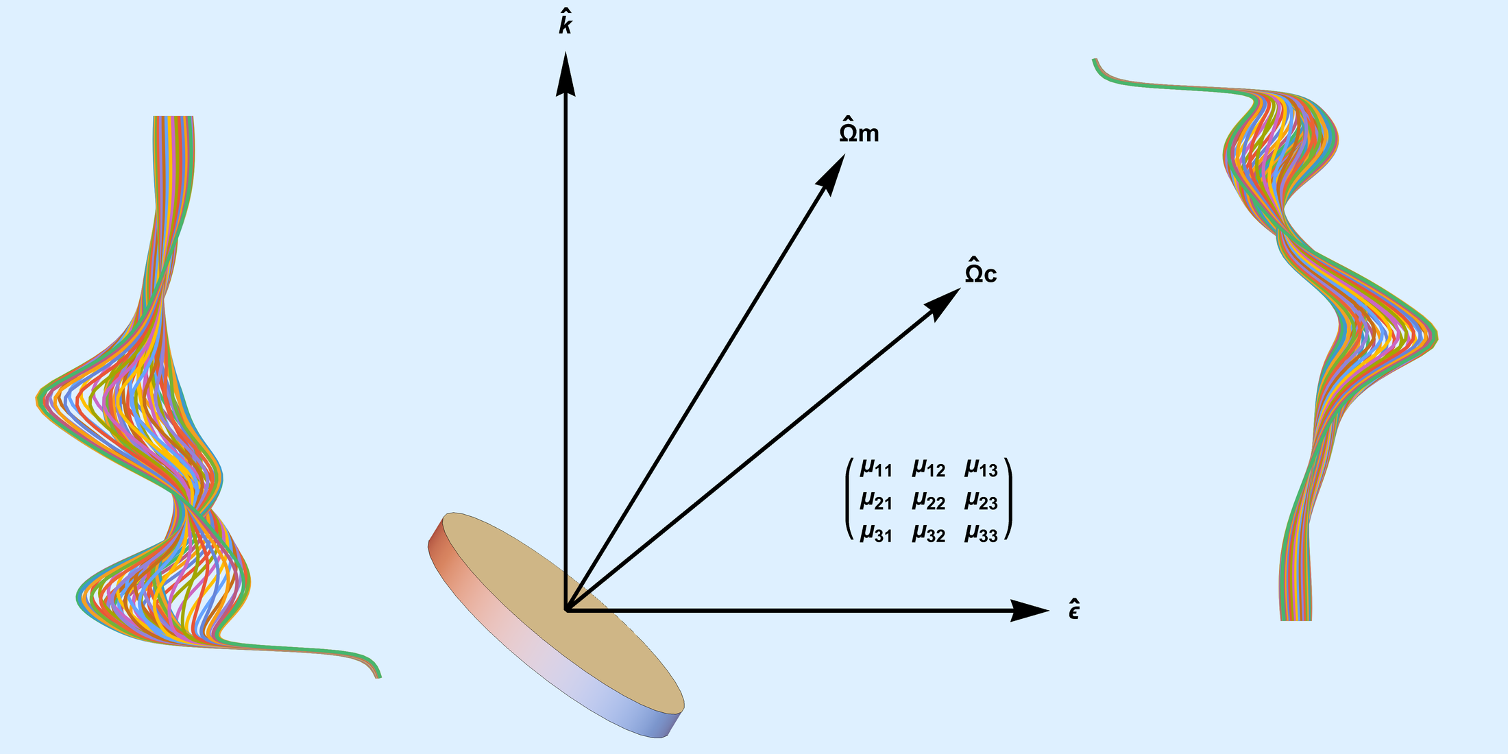
1. Introduction

It is well-known in various types of optical spectroscopy [1,2,3,4,5] that, for oriented samples, additional information (relative to unpolarized beams) can be provided by measuring spectral dichroism with a linearly polarized photon beam. This is clear from fundamental quantum theory [6,7,8] about the interaction of light with matter, and it has been used productively in thousands of papers in many contexts, particularly in the UV–Visible region (in biochemistry and biophysics), and in the X-ray region (in materials physics, geochemistry, condensed matter, and biophysics), e.g., [4,5,9,10,11].

The purpose of this paper is to explain the conceptual basis and theory underpinning our proposed FTMAPS method, as well as the data-to-tensor numerical reconstruction process, and to demonstrate its stability and accuracy using synthetic X-ray absorption data. A strict separation is maintained between two phases: on the one hand, the generation of the synthetic experimental data sets (using FEFF) corresponding to a spinning sample with specific spin axis orientations; and, on the other hand, in a separate process, using only those virtual data, constructing the full dipole absorption tensor as a function of energy, using the tensor to predict the XAFS spectra for arbitrary polarization vectors not necessarily in the original data set, and testing/validating those predicted spectra using FEFF once again to calculate the spectrum for those polarization vectors, which in general were not involved in generating the original virtual data. This is not tautological or circular, but it does show the correctness of the process, within the dipole approximation.

In some of these tests shown below, synthetic random noise is added to demonstrate the stability and accuracy of the experimental data → tensor inversion process. A brief mathematical analysis of one type of systematic error, a sample thickness gradient, is presented; methods for avoiding certain others are offered. Although some experimental aspects of FTMAPS are briefly discussed, for reasons of the scope and size of this paper, detailed experimental implementation issues and experimental validations are deferred to future publications. We invite others to participate in its development.

The theory of the angle dependence of X-ray absorption [5,12] has been comprehensively worked out by Brouder [13], with many references to prior work in his paper. In our current paper, although we will be specifically addressing X-ray Absorption Fine Structure measurements, our same approach is expected to be applicable to other photon energies, e.g., UV–Vis, IR, microwave, or THz spectroscopy, provided the dimensions of the absorbing object (chromophore) are much lower than the wavelength.

Unless otherwise noted, we make use of the dipole approximation. Owing to the short wavelength of X-rays, it is known that quadrupole effects can be non-negligible in the pre-edge region of XAFS spectra, particularly for transition metals, so our approach here is most applicable to such systems over the rising part of the absorption edge and above it, or for the majority of other systems that do not have significant quadrupole effects. In such cases where the dipole approximation is valid, the absorption probability transforms under rotations as a second-rank Cartesian tensor. Below, we make a rough estimate of an upper limit on quadrupole transitions relative to dipole transitions for X-ray absorption.

For a low-symmetry sample, in principle, up to six times as much information can be obtained compared to an isotropically averaged sample (e.g., most solutions, samples consisting of isotropically oriented microcrystals) or samples in which the absorbing sites have cubic point group symmetry (e.g., exact octahedral or tetrahedral symmetry). This is a consequence of there being six distinct values that make up a symmetric 3D Cartesian tensor. Each of these six unique tensor elements is a function of energy.

X-ray linear dichroism, also known as “Polarized XAFS”, has been very productively used in systems in which there is a preferred axis such as the normal to a planar surface to which the molecules are aligned, but may be cylindrically randomly oriented or have a 3-fold or greater axis of symmetry about the surface normal. In such a case, the absorption spectra with polarization along the direction normal to the surface, and parallel to the surface, are usually quite different.

For crystalline samples for which much is known from X-ray diffraction, such as the space group symmetry, and crystal axis orientations as mounted in a goniometer, the additional information can guide the selection of appropriate orientation angles in which to measure the absorption spectrum. Interpreted through a spherical tensor description, excellent work has been done, e.g., [11,13]. The tensor elements can be reconstructed with fewer measurements in such cases because a simplified angle dependence is already known. In FTMAPS, such additional prior knowledge from XRD and spherical tensor theory is not required. It is also applicable to noncrystalline systems.

Despite the extra information linear dichroism (LD) can offer, it is fully used less often than it could be, in part because of the additional experimental complexity and additional data acquisition time required to do the measurements (if measured in conventional ways). These involve 4-circle goniometry, and practical considerations such as sample morphology and other instrumental effects come into play, because different profiles are presented to the beam and sample thickness along the direction of beam propagation generally will vary with orientation, meaning that it needs to be taken into account. It is understandable why most experimentalists simply do not bother with such experiments.

Even so, linear dichroism is not something that can just be ignored. If the X-ray absorption sites (whose intrinsic absorbances have their own angular dependence) have, in addition, a higher-level statistical orientational organization within the sample (i.e., “texture”, “preferred orientation”), then systematic errors can occur if it is ignored. Fortunately, in many cases, one already has, or can prepare, a flat or film sample, in which case the systematic errors usually can be eliminated by magic angle spinning [14,15]. This involves spinning a sample (e.g., film) about an axis that makes the “magic angle” (explained below) with respect to the electric polarization vector of the photon beam assumed as linearly polarized. This has the effect of averaging out the undesired spurious angular contributions to give a signal proportional to the 3D isotropically averaged spectrum, which is what is usually sought. Our proposed method here is a natural but nontrivial extension of magic angle spinning; it delivers the same information, and much more, by also measuring the pair of angles (magic angle ${\theta }_m$ and its complement $\pi /2-{\theta }_m$), whence the name “Full Tensor Magic Angle Pair Spectroscopy”. Instead of merely averaging out unwelcome contributions to the signal, as in normal magic angle spinning, it flips the process on its head to use a specific pair of spin axis orientations to determine the full-dipole-tensor absorption tensor as a function of energy (or wavelength).

In this paper, we use $\mu$ to refer to the spectra and M as the tensor giving rise to them. The X-ray absorption coefficient $\mu \left(\mathcal{E}\right)$ is given by time-dependent perturbation theory [7,8,16,17,18] as

$$\mu \propto {\left|\sum _f\langle f|(\widehat{ϵ}·\overrightarrow{r})e^{i\overrightarrow{k}·\overrightarrow{r}}|i\rangle \right|}^2\approx {\left|\sum _f\langle f|(\widehat{ϵ}·\overrightarrow{r})(1+i\overrightarrow{k}·\overrightarrow{r}\dots )|i\rangle \right|}^2$$

(1)

where $|i\rangle$ is the initial state, $|f\rangle$ are the final states, $\overrightarrow{k}$ is the k-vector of the incoming plane-polarized photon beam, and $\overrightarrow{r}$ is the coordinate over which to be integrated. The first term in the expansion in Equation (1) is the dipole term, and the second gives the quadrupole term, which we treat as negligible here unless otherwise noted.

1.1. Estimate of the Relative Importance of Quadrupole vs. Dipole Transitions

We can make a rough estimate of the ratio of (allowed) quadrupole transitions to (allowed) dipole transitions. Either can be zero for some states, because of symmetry; for our estimate here, we presume this is not the case. The quadrupole transitions are sometimes observable in XAFS in spectral regions and geometries where otherwise-dominant dipole transitions may be forbidden. For a K-edge (or $L_1$, in the pre-edge region), if there is structural inversion symmetry of the sites, the states below the edge will contain no p-symmetry character, and dipole transitions will be forbidden in that region. If there are other states of appropriate symmetry such that quadrupole transitions are allowed, they may be observed, unmasked by dipole transitions. On the edge and above, dipole absorption predominates because there are always allowed symmetry states in the continuum. Similar considerations apply to other absorption edges.

In this subsection, for convenience, we use atomic units, in which ℏ, electron mass m and charge e ($e^2\equiv q^2/(4\pi {ϵ}_0$ in SI units) are all equal to 1. In atomic units (au), the length unit is Bohr radius $a_0$ and the energy unit is Hartree $=2$ Ryd $\approx 27.2$ eV. The dimensionless fine structure constant $e^2/(\hslash c)\approx 1/137.036$, which implies that, in atomic units, the speed of light $c\approx 137$.

The relative magnitudes of the dipole and quadrupole matrix elements above evidently are 1 and $ka$, where a is a measure of the size of the initial state ($1S$ for K-edges). This is clear if one thinks of the matrix element as an integral: the size of the initial state wave function limits the range of the integral. $kc$ is the energy of the photon, which is approximately the absorption edge energy. The initial state is, to a good approximation, that of a hydrogenic atom of atomic number Z. In atomic units, we then have $a\approx 1/Z$ and the energy $kc\approx Z^2/\left(2n^2\right)$, so $ka\approx Z/(2·137)(1/n^2)$, where n is the principal quantum number of the initial state ($n=1$ for K-edges, $n=2$ for L-edges). For Fe ($Z=26$) and K-edge ($n=1$), this gives $\approx 10\%$. The absorption probability scales with the square of the matrix elements, so a rough estimate of the ratio of the allowed quadrupole transition to allowed dipole is about $1\%$. This comports with the observed experimental magnitudes where the allowed quadrupole (in the pre-edge region) of first row transition metal complexes are roughly $1\%$ of the allowed dipole (the edge step). This primitive estimate indicates that the relative importance of quadrupole transitions should grow as $Z^2$: the ratio for Ru K-edge would be roughly three times greater.

1.2. Dipole Absorption Tensor

Having estimated the relative magnitude of quadrupole terms, and taking just the dipole term, we can write Equation (1) as $\mu \propto \widehat{ϵ}·M·\widehat{ϵ}$, where M is a second-rank Cartesian tensor. Writing in spherical coordinates $\widehat{ϵ}=(sin\theta cos\varphi ,sin\theta sin\varphi ,cos\theta )$, we have

$$\begin{array}{cc}\hfill \mu \propto & M_{11}{sin}^2\left(\theta \right){cos}^2\left(\varphi \right)+M_{22}{sin}^2\left(\theta \right){sin}^2\left(\varphi \right)+M_{33}{cos}^2\left(\theta \right)+\hfill \\ \hfill & M_{12}{sin}^2\left(\theta \right)sin\left(2\varphi \right)+M_{23}sin\left(2\theta \right)sin\left(\varphi \right)+M_{31}sin\left(2\theta \right)cos\left(\varphi \right).\hfill \end{array}$$

(2)

Equation (2) represents the basic angular dependence vs. polarization vector orientation of a single absorbing site, typically a molecular chromophore (e.g., Heme group in a protein), or an oriented crystallite within a material. It is universal, within the dipole approximation, in X-ray, UV–Vis, IR, THz, and Microwave wavelengths. The dipole approximation applies when the dimensions of the absorbing center are much smaller than the wavelength of the EM wave.

1.3. Averaging over the Sample

The absorption of an “elementary chromophore” or crystallite has the form given in Equation (2), but needs to be averaged over the various sites contained within the sample. The orientations of each of these may vary because of inequivalently oriented sites within a single crystal, or different crystallites or domains with varying orientations within the sample. We regard these as reoriented copies of the elementary M tensor over which to be summed.

A second-rank tensor transforms as the outer product of two vectors; rotating a second-rank tensor can be accomplished by sandwiching the tensor matrix between a rotation matrix $R({\omega }_f,{\omega }_i)$ and its transpose $R^T({\omega }_f,{\omega }_i)=R({\omega }_i,{\omega }_f)$, where ${\omega }_i$ and ${\omega }_f$ are the initial and final orientations. The result of averaging a second-rank tensor is still a second-rank tensor, but with possibly reoriented principal axes and altered principal values. Summing up such rotated tensors, weighted according to a probability distribution $P({\omega }_f,{\omega }_i)$ characteristic of the sample, can be written $\overline{M}=\int P({\omega }_f,{\omega }_i)R({\omega }_i,{\omega }_f)·M·R({\omega }_f,{\omega }_i)d{\omega }_f$, where “·” indicates matrix multiplication, with the initial orientation ${\omega }_i$ fixed. The result $\overline{M}$ also transforms under rotations as a second-rank tensor, but not generally with the values of the original prototype M. In component notation, we can write the average as ${\overline{M}}_{jk}=\left(\int P({\omega }_f,{\omega }_i){\mathcal{R}}_{jklm}({\omega }_f,{\omega }_i)d{\omega }_f\right)M_{lm}$, where ${\mathcal{R}}_{jklm}$ is a fourth-rank tensor relating the two second-rank tensors, and we implicitly sum over repeated indices.

We call $\alpha$ the angle of rotation of the sample about the rotation axis. In our development here, we specify that the sample is homogeneous, as in a uniform film.

The only $\alpha$-dependence of the measured absorption is the underlying elementary tensorial angle dependence as in Equation (2), owing to the molecular or crystalline structure. However, if the sample consists of many crystallites that may themselves be oriented in various nonrandom ways, it is possible for a sample to acquire an additional $\alpha$-dependence. If this is present, it would need to be characterized and corrected for.

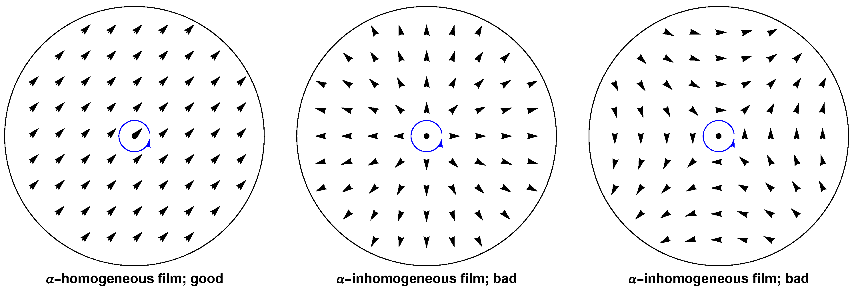
In this paper, we consider samples in which the only angle dependence is due to the “elementary chromophore” or crystallite, and no additional $\alpha$-dependent structure in the sample is present. This will be the case if the sample is angularly ($\alpha$)-homogeneous, as schematically shown in the left schematic diagram in Figure 1. The arrows indicate the orientations of elementary chromophores or crystallites. If this sample were rotated, the underlying chromophore/crystallites would rotate in the way assumed here as in Equation (2). In contrast, in the sample represented by the middle diagram of Figure 1, under rotation by an angle $\alpha$, the orientation of the measured elementary chromophores/crystallites would not change upon rotation, as is expected. The orientation of the crystallite/chromophore illuminated within the beam spot after the rotation by $\alpha$ would be the same as it was before the rotation. The rightmost graphic in Figure 1 shows a more complicated distribution.

This homogeneity criterion may appear to be more restrictive than it actually is. A translationally uniform sample is suitable, and many such films are produced this way in a continuous process, by default. Any angular structure that is independent of $\alpha$ does not cause any difficulties and, importantly, such effects can be averaged out by magic angle spinning [14,15].

1.4. Magic Angle Spinning to Average out Anisotropies

In the most basic XAFS measurements, such as uniform polycrystalline or amorphous powders, alloys, or solutions, it is often presumed that the local structure is isotropically averaged over the sample. The material may consist of small oriented grains, but the common assumption is the orientations of these average out isotropically. This, of course, is not necessarily the case. If particles in a sample have a preferred orientation, there will be residual dichroic effects that result in systematic errors. Fortunately, there is a simple way to eliminate this problem: magic angle spinning [14,15].

Consider a homogeneous sample with a flat surface that can be rotated around the surface normal. In this subsection, we choose our spherical coordinate system so that its polar axis ($\theta =0$) is aligned with the rotation axis $\overrightarrow{\mathsf{\Omega }}$. If we then average the signal, which varies according to Equation (2), over a full $\varphi$ rotation, we obtain an average that is proportional to

$$\mu \propto \left(M_{11}+M_{22}\right){sin}^2\theta +2M_{33}{cos}^2\theta$$

(3)

In Equation (3), selecting $\theta$, which here is the angle between the spin axis and the electric polarization vector $\overrightarrow{ϵ}$, to be the “magic angle” ${\theta }_m=arccos(1/\sqrt{3})=arctan\sqrt{2}\approx 54.7356deg$ gives a result $\mu \propto (M_{11}+M_{22}+M_{33})$. This is also proportional to the isotropic average

$${\int }_0^{2\pi }{\int }_0^{\pi }\widehat{ϵ}·M·\widehat{ϵ}sin\theta d\theta d\varphi ,$$

which is what is normally sought in XAFS experiments.

We conclude that averaging the signal while rotating about an axis that is at an angle ${\theta }_m$ with respect to the electric polarization vector gives a result that is proportional to what would be obtained by averaging over a sphere. This special geometrical property is the reason ${\theta }_m$ is called the “magic” angle, a term originating in NMR spectroscopy.

It is important to realize that this is true regardless of how the elementary absorbing chromophore/crystallite is oriented relative to the sample normal. The magic angle average above is proportional to the trace (sum of diagonal elements) of M. Since the transpose of a rotation matrix is also its inverse matrix, the rotation transformation of the tensor also is a similarity transformation, and the trace of a matrix is invariant under similarity transformations. This implies that, if the elementary chromophore were pre-rotated to some different orientation, its trace, and therefore also the magic angle average, would be unchanged. The chromophore orientation relative to the surface normal does not affect the magic angle average. This point is sometimes misunderstood, which unfortunately may have limited the productive use of magic angle spinning.

Magic angle spinning eliminates any spurious dichroism there might be owing to residual preferred orientation within the sample. We note parenthetically that only three or more equally spaced angles in $\alpha$ are needed to accomplish this averaging effect, but in this paper we find that we can do much more with it than just calculate the average.

1.5. Full-Tensor Magic Angle Pair Spectroscopy

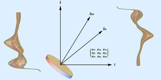
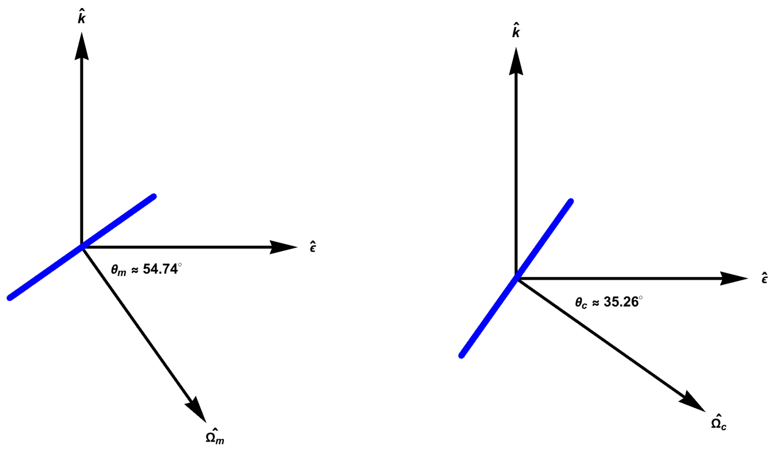
For simplicity and concreteness, we take $\widehat{ϵ}=(1,0,0)$, i.e., the polarization along the x direction, and the rotation axis in the $x,z$ plane, as shown in Figure 2, so $\hat{\mathsf{\Omega }}=(\sqrt{{\displaystyle \frac{1}{3}}},0,\sqrt{{\displaystyle \frac{2}{3}}})$. We make use of Mathematica’s [19] RotationMatrix function to generate the transformation matrix for a rotation by angle $\alpha$ around the $\hat{\mathsf{\Omega }}$ vector, which can be written as

$$\left(\begin{array}{ccc}{\displaystyle \frac{1}{3}}(2cos\left(\alpha \right)+1)& -\sqrt{{\displaystyle \frac{2}{3}}}sin\left(\alpha \right)& -{\displaystyle \frac{1}{3}}\sqrt{2}(cos\left(\alpha \right)-1)\\ \sqrt{{\displaystyle \frac{2}{3}}}sin\left(\alpha \right)& cos\left(\alpha \right)& -{\displaystyle \frac{sin\left(\alpha \right)}{\sqrt{3}}}\\ -{\displaystyle \frac{1}{3}}\sqrt{2}(cos\left(\alpha \right)-1)& {\displaystyle \frac{sin\left(\alpha \right)}{\sqrt{3}}}& {\displaystyle \frac{1}{3}}(cos\left(\alpha \right)+2)\end{array}\right)$$

(4)

We then can rotate the M tensor by sandwiching it between this rotation matrix and its transpose to obtain an expression that contains only multiples of the five basis functions $(1,cos\left(\alpha \right),sin\left(\alpha \right),cos\left(2\alpha \right),sin\left(2\alpha \right))$. The (Fourier) coefficients of these basis functions themselves depend on specific linear combinations of the M tensor elements. These are given in

Table 1. Relation between dipole tensor elements and Fourier coefficients for magic angle orientation; $\widehat{ϵ}=(1,0,0)$; $\alpha$ is the angle of rotation about the spin axis $\overrightarrow{\mathsf{\Omega }}$. Note the angular constant term (coefficient of 1) is the isotropic average value normally sought in XAFS. Expressions computed in Mathematica [19].

Basis Function	Symbolic Coefficient
1	${\displaystyle \frac{1}{3}}\left(M_{11}+M_{22}+M_{33}\right)$
$cos\left(\alpha \right)$	${\displaystyle \frac{2}{9}}\left(2M_{11}+\sqrt{2}{M}_{31}-2M_{33}\right)$
$sin\left(\alpha \right)$	$-{\displaystyle \frac{2}{9}}\left(\sqrt{6}{M}_{12}+2\sqrt{3}{M}_{23}\right)$
$cos\left(2\alpha \right)$	${\displaystyle \frac{1}{9}}\left(2M_{11}-3M_{22}-2\sqrt{2}{M}_{31}+M_{33}\right)$
$sin\left(2\alpha \right)$	$-{\displaystyle \frac{2}{9}}\left(\sqrt{6}{M}_{12}-\sqrt{3}{M}_{23}\right)$

for the ${\theta }_m$ magic angle orientation. We also find it useful to compute the corresponding coefficients for the rotations around ${\theta }_c$, the complement to the magic angle ${\theta }_c\equiv {\displaystyle \frac{\pi }{2}}-{\theta }_m$ given in

Table 2. Relation between dipole tensor elements and Fourier coefficients for complementary angle orientation; $\widehat{ϵ}=(1,0,0)$; $\alpha$ is the angle of rotation about the spin axis $\overrightarrow{\mathsf{\Omega }}$. Expressions computed in Mathematica.

Basis Function	Symbolic Coefficient
1	${\displaystyle \frac{1}{6}}\left(3M_{11}+M_{22}+2\left(\sqrt{2}{M}_{31}+M_{33}\right)\right)$
$cos\left(\alpha \right)$	${\displaystyle \frac{2}{9}}\left(2M_{11}-\sqrt{2}{M}_{31}-2M_{33}\right)$
$sin\left(\alpha \right)$	$-{\displaystyle \frac{2}{9}}\left(2\sqrt{3}{M}_{12}+\sqrt{6}{M}_{23}\right)$
$cos\left(2\alpha \right)$	${\displaystyle \frac{1}{18}}\left(M_{11}-3M_{22}-2\sqrt{2}{M}_{31}+2M_{33}\right)$
$sin\left(2\alpha \right)$	${\displaystyle \frac{1}{9}}\left(\sqrt{6}{M}_{23}-\sqrt{3}{M}_{12}\right)$

.

In an experiment, one can directly determine the numerical coefficients of each of these basis functions at each energy. Once found, these form a linear system of equations by which the values of the tensor elements of M can be determined. In the general case of no symmetry, six values are needed to fully determine the tensor at each energy, but these equations only provide five. But, if an independent measurement is done at another angle (say, ${\theta }_c$), then ten numbers are available, which is more than enough to determine the six unique elements of the M tensor in a least-squares sense. The “extra” parameters could be used to manage experimental uncertainties such as background shifts or similar real-world complications, but it is best to eliminate those experimentally. We do not get into such details here, as we aim to demonstrate the potential of this technique. We consider here the experimental geometry shown in Figure 2.

Determining these Fourier coefficients experimentally can be done in many ways. The constant term (the coefficient of the basis function in Equation (1)) is just the average value, which is what we seek for an isotropically averaged signal, as in ordinary magic angle spinning, of which FTMAPS is a nontrivial extension. They could be determined by analog filtering and sampling with an A/D converter, followed by numerical dot product (as we do here, below), or by digital bandpass filtering or lock-in methods. Some other options can be found in the Discussion section. Most of these can be done relatively inexpensively using modern electronics. Even discrete stepping in angle instead of continuous spinning is a feasible approach. Alternatively, the data could be simply recorded and processed afterward, as we illustrate in the Materials and Methods section.

The key point is that only the rotation of the sample about two discrete spin axes is needed to robustly determine the full absorption tensor, and potentially can be done in only a little more time than a few normal energy scans. In the next section of this paper, we demonstrate this by doing a series of simulated experiments. We compute the spectra that would be obtained while rotating the sample in this way, treating the result as virtual experimental data, reconstructing the full $M\left(\mathcal{E}\right)$ tensor as a function of energy from it, and, to test it, comparing the projections of the predicted tensor along arbitrarily chosen polarization directions with explicit calculations at that polarization, using the reference theoretical code FEFF [20]. We find excellent agreement in all cases.

2. Materials and Methods

2.1. Computations Using FEFF

FEFF [20], a very well-established theoretical XAFS code, was used to compute simulated XAFS spectra as a function of energy for a series of illustrative structures and appropriately selected polarization vectors. FEFF8.4 version was used, which is written in Fortran 77. It was compiled in gfortran (GCC15) at optimization level 1 for Mac OS 26.5 on M2 Max MacBook Pro hardware (Apple Computer, Cupertino California, USA). This is not the most sophisticated use of the FEFF series of codes, but it is more than sufficient for our purposes here.

The program was run in XANES Full Multiple Scattering (FMS) mode, which calculates the near-edge region of the XAFS spectrum. XANES often shows interesting variations in structure, but similar calculations can be done with EXAFS, both with multiple coordination shells. Self-consistent potentials were not used here because they are irrelevant for our purpose (it is commented on in the example). The dipole approximation, however, is made in the FEFF calculations, as is discussed previously. An example feff.inp file is shown below. A template string of this sort was used to automatically generate a series of jobs in which the positions of all the atoms were rotated by the variable angle $\alpha$ around the spin axis $\hat{\mathsf{\Omega }}$.

For each run, first, a prototype local atomic structure was built, with the option to randomly perturb atomic positions so as to break all local point group symmetries, or to preserve various symmetries. Here, we use a central Mn atom surrounded by 6 (or 5) oxygen atoms at various locations. No special point group symmetry or orientation is assumed, except as indicated for certain tests shown below.

Here is a sample FEFF input file:

Mn central atom, Oxygen neighbors, distorted octahedral coordination,

polarization vector (1,-2,1). This form is used to validate the computed

spectrum, synthesized from the reconstructed $M$ tensor, along that

direction.   For generating the simulated experimental  data, polarization

is fixed at (1,0,0) for all runs while the atom coordinates are rotated.

-------------------------------------------------------------------------

TITLE Illustration of Magic Angle Spinning

EDGE K 1.0

CONTROL 1 1 1 1 1 1

*SCF 3.0 1

FMS 3.0 1

XANES 8.0 0.05

Polarization  1 -2 1

POTENTIALS

*ipot z label

0 25 Mn

1 16 O

ATOMS

*x y z ipot atom

0. 0. 0. 0 Mn

-1.550676656607681 0.5279844219748255 -0.3677425161328711 1 O

1.7222347900324142 -0.12287594786724987 -0.45252829065425026 1 O

-0.05559267001253487 -1.3949939627430388 -0.07222041064169282 1 O

-0.11900081923005112 2.1574028343591256 -0.11666143758592029 1 O

-0.5190776083591475 0.28615541317596893 -2.5209783909703383 1 O

-0.7590753880744365 0.031062973781723624    2.225967883900838         1 O

END

To simulate the experiments, a series of FEFF [20] 8.4 calculations was run to calculate the spectra as a function of rotation angle $\alpha$ around the spin axis $\overrightarrow{\mathsf{\Omega }}$. The same effect presumably could be produced more easily by changing the polarization vector specified in the feff.inp file, but this approach is perhaps more intuitive, albeit more cumbersome: it corresponds to physically rotating the sample and the atoms within it. The coordinates of all the atoms were rotated using appropriate rotation matrix for the given $\alpha$ about $\hat{\mathsf{\Omega }}$.

Operationally this was orchestrated within Mathematica [19], with our code that generates a FEFF input file (derived from a template string in the code), followed by writing out the file, executing FEFF by Mathematica’s RunProcess, reading in the resulting FEFF-generated xmu.dat file, and repeating over $\alpha$ values. This results in a Mathematica data structure consisting of spectra as a function of both energy and rotation angle $\alpha$ about axis $\overrightarrow{\mathsf{\Omega }}$. In the results shown here, 60 equally spaced values of $\alpha$ were used; the whole process of synthesizing the bundle of 60 spectra takes about 18 s (run as a serial process) on a MacBook Pro M2 Max laptop computer.

2.2. Determining the Absorption Tensor from the Simulated Experimental Spectra

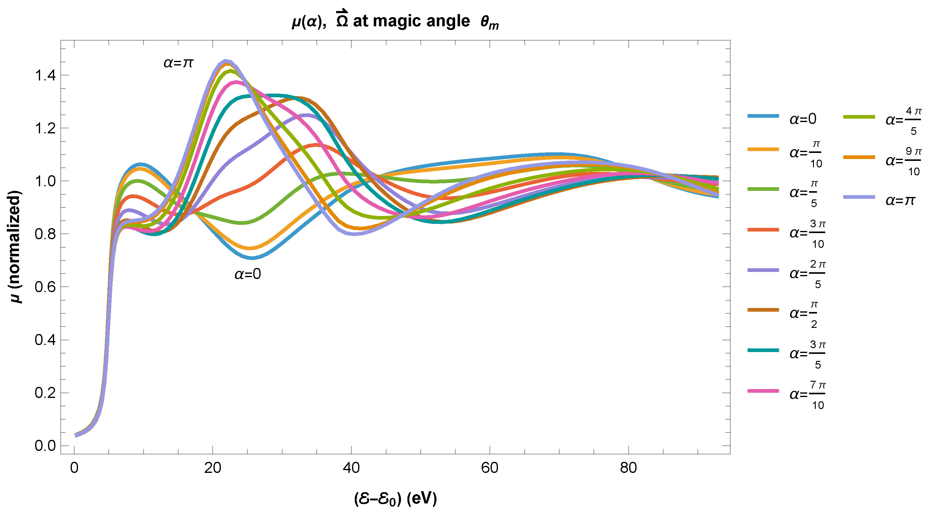
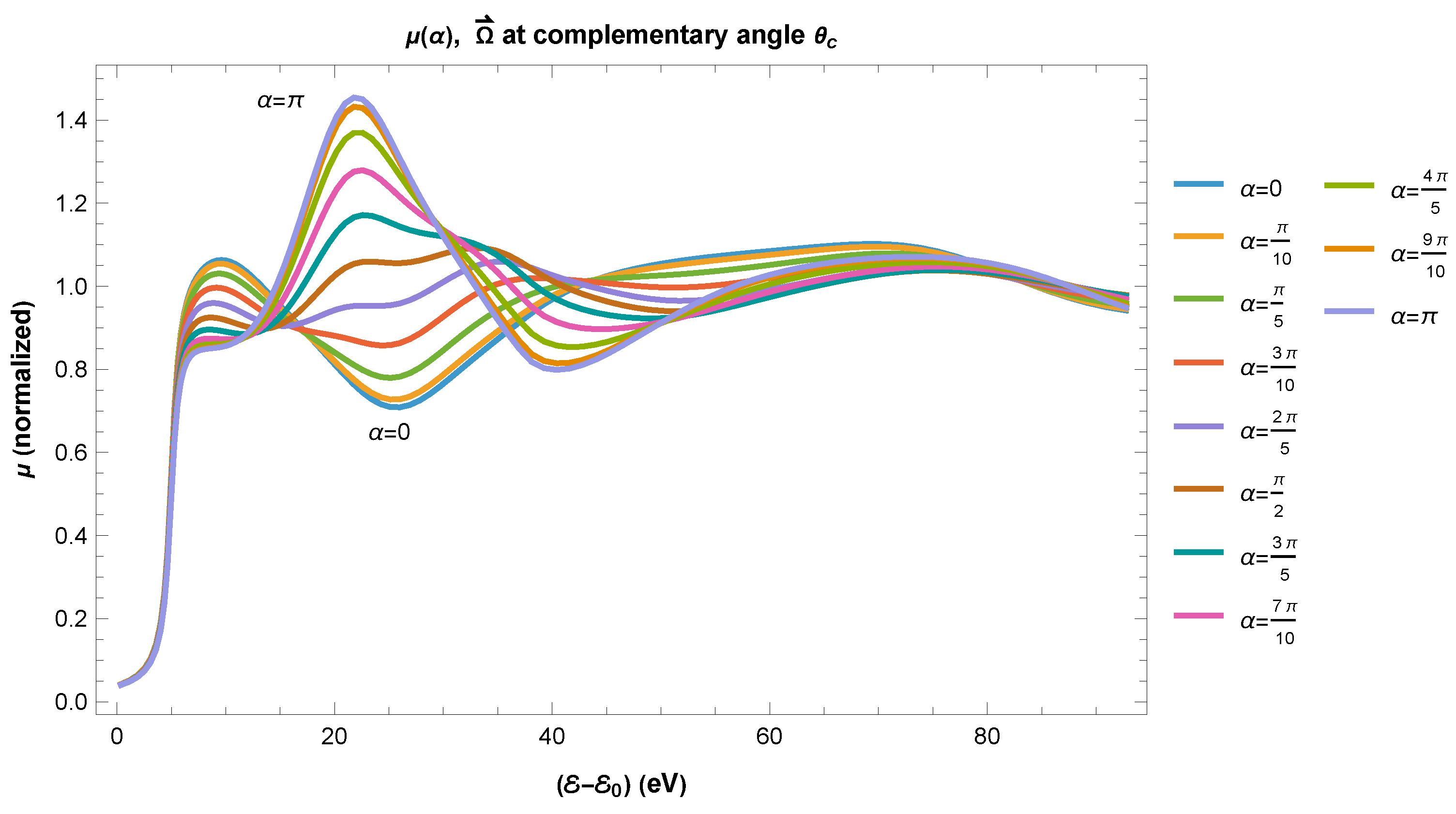
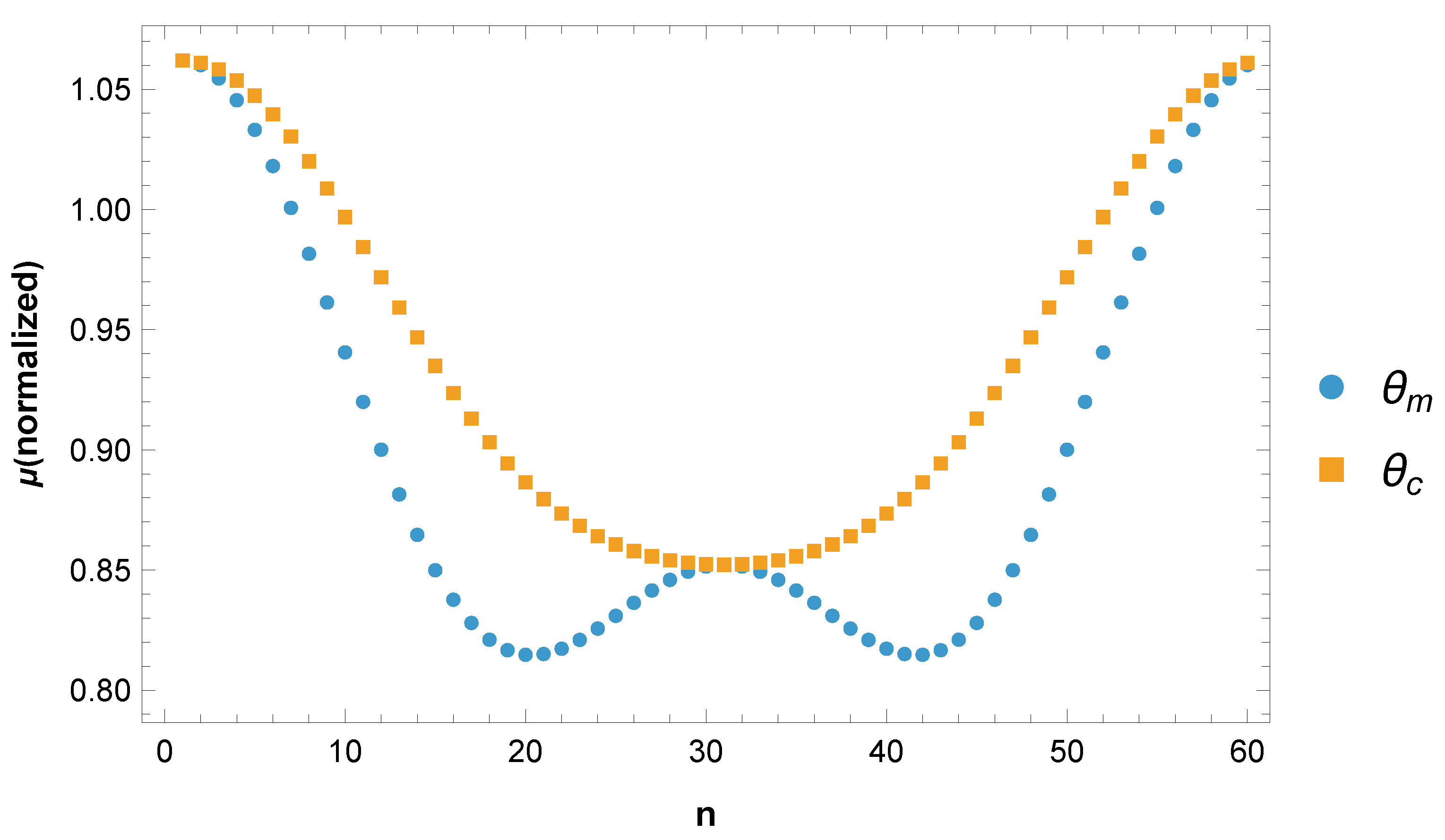
For a fixed energy value, the data are simply a function that is uniformly sampled in angle $\alpha$ 60 times between 0 and $2\pi$. Such spectra are similar to those in Figure 3, but more densely sampled in $\alpha$; each structure generates a pair of such spectral bundles. The choice of 60 values used here is representative, but is not critical as long as there are more than 5, and preferably considerably more if substantial noise is present in the data, so as to oversample and reduce the aliasing of noise power. 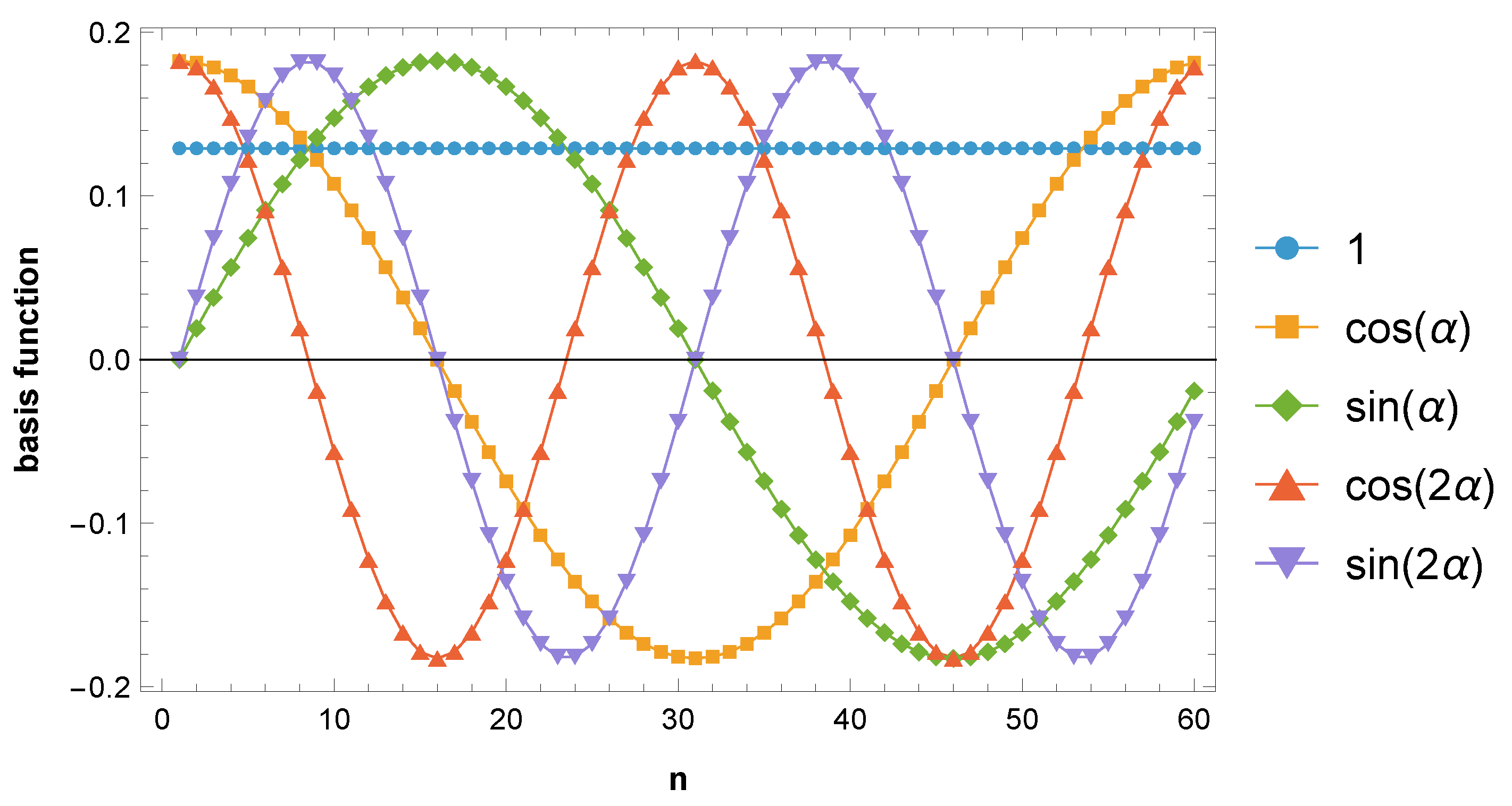An example of the sampled $\alpha$ dependence for ${\theta }_m$ and ${\theta }_c$ is shown in Figure 4. The basis functions are evaluated at each angle to produce a vector (1D array) (as shown in Figure 5), and the dot products between these vectors and the sampled data immediately give the numerical Fourier coefficients (once normalized by $1/\sqrt{30}$ for the trig functions and $1/\sqrt{60}$ for the unit basis function). Other frequency components such as noise that might be present in experimental data that are multiples of this base frequency are orthogonal to these, and produce zero.

A set of these numerical coefficients is determined at each energy. In the first implementation, as shown, they are equated to expressions given in Table 1 (for ${\theta }_m$) and Table 2 (for ${\theta }_c$), and the resulting linear equations numerically solved for the unknown tensor elements at each energy. The linear system is overdetermined (10 equations for 6 unknowns) so the sum of squares of the differences between corresponding tensor elements of the two estimates of the M matrix is numerically minimized, and the two tensor solutions are averaged to produce the final estimate.

Alternatively, this can be accomplished using a Moore–Penrose pseudo-inverse, as described further in the next subsection, here implemented with Mathematica’s PseudoInverse function. This is done at each energy value, so the final result is a tensor-valued function of energy—in the case shown here, on a grid of 100 energy points. The choice of 100 here is not important; for EXAFS, it would be several times larger, or, for XANES, it could be smaller. The Moore–Penrose PseudoInverse approach is described in the next subsection in more detail. It is more direct and efficient, and gives equivalent results to the method described here.

The computations at each energy are independent of each other. If certain regions of energy are flawed (e.g., crystal glitches) or questionable (for example, significant quadrupole effects are present), they can simply be omitted—any errors in them do not propagate to other energy points. The total execution time to construct the estimated tensor for all energies using the (precomputed) virtual experimental spectra by this method is about 1.5 s on an M2 Max MacBook Pro laptop computer.

In more granular detail, the process we have used is as follows. For a specified spin axis (say, ${\theta }_m$), we select a slice of the data at a particular energy. This slice gives us $\mu$ as a function of $\alpha$ that is uniformly sampled 60 times over a full rotation, which yields a numerical list/array/vector, that we next wish to decompose in a Fourier series as a function of $\alpha$. The basis functions $(1,cos\left(\alpha \right),sin\left(\alpha \right),cos\left(2\alpha \right),sin\left(2\alpha \right))$ are uniformly sampled on the same $\alpha$ grid of 60 points from $\alpha =0$ to $2\pi$ as the data. The dot product between the experimental-data-vs-$\alpha$ vector and a particular basis function, when scaled by 1/60 for the unit basis function 1, or $\sqrt{2}/60$ for the trigonometric basis functions, directly gives the coefficient for that specific Fourier component of the signal vs. $\alpha$ at that energy. This is repeated for each of the basis functions. The numerical values obtained this way are then equated to the corresponding symbolic expressions given in Table 1 and Table 2, which can then be solved for the unknown tensor elements at the chosen energy. This process is done for both angles ${\theta }_m$ and ${\theta }_c$. In an experimental measurement, the samples vs. $\alpha$ could be saved to be processed this way during later analysis. Alternatively, the Fourier decomposition could be done at the beamline and saved as five numbers per energy, one for each basis function, or as the amplitude and phase of the relevant frequency components. These are the experimental data that are needed; examples of the full set of absorption curves vs. $\alpha$ and energy are shown in Figure 3.

At a given energy, in general, we have six unknown variables, which are the six unique elements of a symmetric second-rank 3D Cartesian tensor. For one orientation (say, ${\theta }_m$) of the spin axis, we can uniquely determine only five of them because there are only five relevant Fourier components in the data, leaving one undetermined tensor element (it does not matter which one). But, by requiring consistency in the tensor elements for the measurements taken at the two orientations ${\theta }_m$ and ${\theta }_c$, and by minimizing the mean square difference between reconstructed tensors as function of the single undetermined matrix element parameter, the tensor is specified at the chosen energy. This calculation, at each energy, is independent of the other energies, and it is looped over to generate the full-tensor spectrum. In this implementation, this process is done in about a dozen lines of code in Mathematica and takes seconds to execute.

2.3. Pseudo-Inverse

Another approach that we also have implemented (with equivalent results to the above, apart from roundoff error) is to write the set of overdetermined linear equations as the matrix product of a $10\times 6$ matrix m multiplied by a length-6 column vector x that is equated to a length-10 column vector b containing the 10 (physically or virtually) measured Fourier coefficients (5 basis functions × 2 spin axis angles). A non-square matrix does not possess an ordinary matrix inverse, but such a matrix can be inverted in a more general sense using a Moore–Penrose pseudo-inverse (PseudoInverse in Mathematica), which is equivalent to finding a minimum-norm least-squares solution as above. In

Table 3. Coefficients of the matrix m relating the 6 unknown symbolic variables (unique elements of the absorption tensor) to the 10 Fourier coefficients to be experimentally determined from the data. The product of this matrix with the 6-element column vector containing symbolic matrix elements is equated to the experimentally determined numerical Fourier coefficients. The tensor elements are in the resulting array in the order $M_{11}$, $M_{12}$, $M_{22}$, $M_{23}$, $M_{31}$, $M_{33}$. The absorption tensor M is symmetric, so $M_{21}=M_{12}$, $M_{32}=M_{23}$, $M_{13}=M_{31}$.

$m=\left(\begin{array}{cccccc}\frac{1}{3}& 0& \frac{1}{3}& 0& 0& \frac{1}{3}\\ \frac{4}{9}& 0& 0& 0& \frac{2\sqrt{2}}{9}& -\frac{4}{9}\\ 0& -\frac{2\sqrt{\frac{2}{3}}}{3}& 0& -\frac{4}{3\sqrt{3}}& 0& 0\\ \frac{2}{9}& 0& -\frac{1}{3}& 0& -\frac{2\sqrt{2}}{9}& \frac{1}{9}\\ 0& -\frac{2\sqrt{\frac{2}{3}}}{3}& 0& \frac{2}{3\sqrt{3}}& 0& 0\\ \frac{1}{2}& 0& \frac{1}{6}& 0& \frac{\sqrt{2}}{3}& \frac{1}{3}\\ \frac{4}{9}& 0& 0& 0& -\frac{2\sqrt{2}}{9}& -\frac{4}{9}\\ 0& -\frac{4}{3\sqrt{3}}& 0& -\frac{2\sqrt{\frac{2}{3}}}{3}& 0& 0\\ \frac{1}{18}& 0& -\frac{1}{6}& 0& -\frac{\sqrt{2}}{9}& \frac{1}{9}\\ 0& -\frac{1}{3\sqrt{3}}& 0& \frac{\sqrt{\frac{2}{3}}}{3}& 0& 0\end{array}\right)$

and

Table 4. Coefficients of the PseudoInverse matrix $m^{-1}$ relating the 10 numerical Fourier coefficients determined experimentally from the data to the 6 unknown variables (unique elements of the absorption tensor). Multiplying this matrix by the array of 10 numerical Fourier coefficients directly gives the numerical tensor matrix elements as a 6-element column vector, in the order $M_{11}$, $M_{12}$, $M_{22}$, $M_{23}$, $M_{31}$, $M_{33}$. The absorption tensor M is symmetric, so $M_{21}=M_{12}$, $M_{32}=M_{23}$, $M_{13}=M_{31}$. The left matrix product $m^{-1}·m$ yields the $6\times 6$ identity matrix.

$m^{-1}=\left(\begin{array}{cccccccccc}\frac{93}{226}& \frac{44}{113}& 0& \frac{133}{226}& 0& \frac{133}{226}& \frac{64}{113}& 0& \frac{53}{226}& 0\\ 0& 0& -\frac{12\sqrt{6}}{187}& 0& -\frac{123\sqrt{\frac{3}{2}}}{187}& 0& 0& -\frac{57\sqrt{3}}{187}& 0& -\frac{39\sqrt{3}}{187}\\ \frac{161}{113}& -\frac{53}{113}& 0& -\frac{161}{113}& 0& -\frac{48}{113}& \frac{77}{113}& 0& -\frac{82}{113}& 0\\ 0& 0& -\frac{6\sqrt{3}}{17}& 0& \frac{15\sqrt{3}}{34}& 0& 0& -\frac{3\sqrt{\frac{3}{2}}}{17}& 0& \frac{3\sqrt{6}}{17}\\ -\frac{483}{452\sqrt{2}}& \frac{249}{226\sqrt{2}}& 0& -\frac{195}{452\sqrt{2}}& 0& \frac{483}{452\sqrt{2}}& -\frac{285}{226\sqrt{2}}& 0& -\frac{93}{452\sqrt{2}}& 0\\ \frac{51}{113}& -\frac{155}{226}& 0& \frac{62}{113}& 0& \frac{62}{113}& -\frac{133}{226}& 0& \frac{40}{113}& 0\end{array}\right)$

below, we give explicit matrices for m and pseudoinverse $m^{-1}$. We note that all of the elements of $m^{-1}$ are numerically between $\pm 161/113\approx 1.43$, so the inverse mapping from Fourier coefficient to absorption tensor matrix is very well-behaved indeed. This structure is independent of the number of spin angles sampled (if Fourier coefficients are determined that way) or the number of energies (wavelengths). This same linear mapping is done separately for the measurements at each energy.

A singular value decomposition (SVD, implemented using Mathematica’s SingularValueDecomposition function) of the m matrix gives six singular values, all of which are on the order of 1 (similar for $m^{-1}$). The condition number, i.e., the ratio of the largest to the smallest singular values, is $\approx 3.36$ for both m and $m^{-1}$, which indicates excellent conditioning of the coefficient matrix m and $m^{-1}$, which is composed of the entries in Table 1 and Table 2, for ${\theta }_m$ and ${\theta }_c$, and the direct and pseudo-inverse matrices are given explicitly in Table 3 and Table 4. The small value of this condition number implies that perturbations to the data from noise or other influences are not substantially amplified by the inversion process in obtaining the tensor elements. Note that this stability is an intrinsic property of the structure of the equations as presented, not the quality of the data. If (for example) the second angle ${\theta }_c$ were chosen to be only slightly different from ${\theta }_m$, the inversion would not have this desirable stability. The determination of the Fourier coefficients from the data is similarly computationally robust, being simply a low-order Fourier series, and projection onto that limited basis set can be viewed as a kind of low-pass digital filtering.

2.4. Predicting Absorption for Arbitrary Polarization Direction

This final estimate of the dipole absorption tensor $M\left(\mathcal{E}\right)$ is our key objective. It can be analyzed in various ways, compared with DFT or other theoretical calculations, and used to predict the absorption for a hypothetical experiment in which the polarization vector is oriented in any chosen direction $\widehat{ϵ}$, simply by evaluating $\widehat{ϵ}·M\left(\mathcal{E}\right)·\widehat{ϵ}$. This is true even for orientations that are experimentally inaccessible, such as direct absorption measurements parallel to the plane of the sample, i.e., perpendicular to the spin axis $\overrightarrow{\mathsf{\Omega }}$. Fluorescence excitation experiments are quite feasible under such circumstances, and FTMAPS would afford an opportunity to compare the two modalities. In many cases, the structure and angle dependence of the fluorescence spectra are the same as in absorbance, but subtleties can arise depending on the time scales of elementary processes [6,21]. Once computed, calculating the absorbance for arbitrary polarization is virtually instantaneous. We find it is very useful for analysis, simulation, and interactive exploration using Manipulate in Mathematica.

3. Results

Here, we present some examples of this procedure on a sequence of simple structures of practical relevance: manganese–oxygen coordination complexes, computed using FEFF in full multiple scattering mode. Our same approach applies equally well for multiple-coordination-shell complexes in the dipole approximation, and, for EXAFS, over an extended energy region.

The sequence of tests is arranged as a set of structures with decreasing degrees of symmetry. We start with exact octahedral symmetry, with oxygen atoms at the vertices of an octahedron centered on a Mn atom. This belongs to a cubic point group, and, as such, there should be no angle dependence at all. For the next structure, we then break octahedral symmetry slightly (to orthorhombic) by keeping the oxygen ligand atoms on-axis in x, y, and z, but vary the distances along each direction, while preserving the inversion symmetry of the site. We then break the inversion symmetry by removing one of the oxygen atoms at the short distance. Next, we break all symmetries by applying pseudo-random displacements in x, y, z to each separate ligand atom. We do this with two sets of pseudo-random displacements. To render the calculation repeatable, if that is desired, we set a random seed of 1538 for the first random structure and 7237 for the second. In these cases, the full-tensor character comes into play.

3.1. Basic Tests

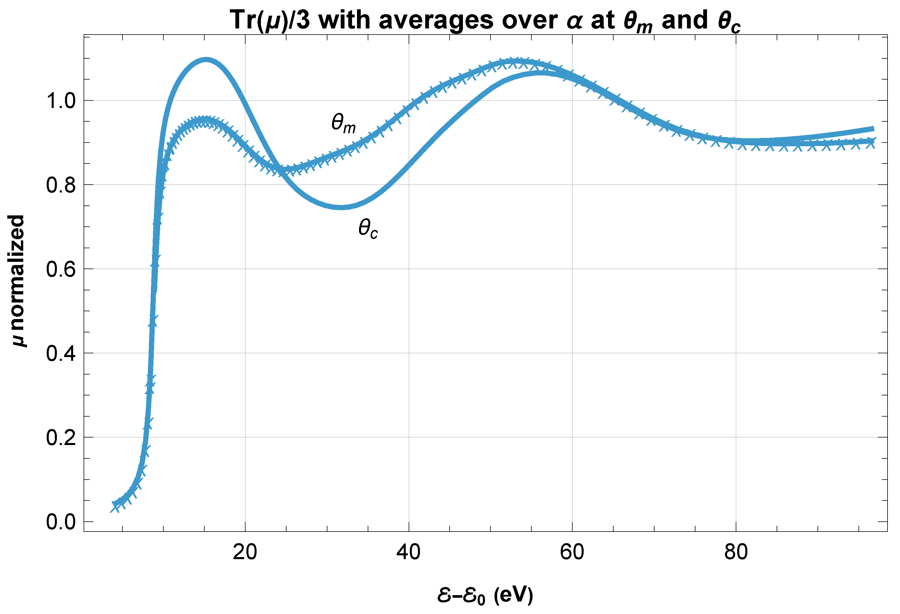
In Figure 6, the averages over all $\alpha$ values of the spectra in Figure 3 are plotted as solid lines. Also plotted (with symbol “x”) is 1/3 of the trace of the reconstructed tensor as a function of energy. The latter agrees precisely with the magic angle average ${\theta }_m$, which is also the isotropic average that is normally sought in XAFS experiments. In contrast, the complementary angle ${\theta }_c$ average is quite different, as expected. The magic angle ${\theta }_m$ is indeed special.

All of the following examples show a spectrum that is computed for a specified electric polarization vector $\overrightarrow{ϵ}$, which corresponds to physically orienting the sample so the polarization is in that direction. In other words, they are simulated experimental spectra generated from the precomputed tensors that were separately computed from (simulated) experimental spectra, as described above.

To test these results, we also ran FEFF calculations in which the polarization vector was oriented in that same direction. This was automated similarly to that described above, but the coordinates were left unrotated, and the polarization direction was changed. We use an unnormalized polarization vector for convenience when specifying the polarization direction—it is normalized internally by our code, and also FEFF. The normalization is immaterial.

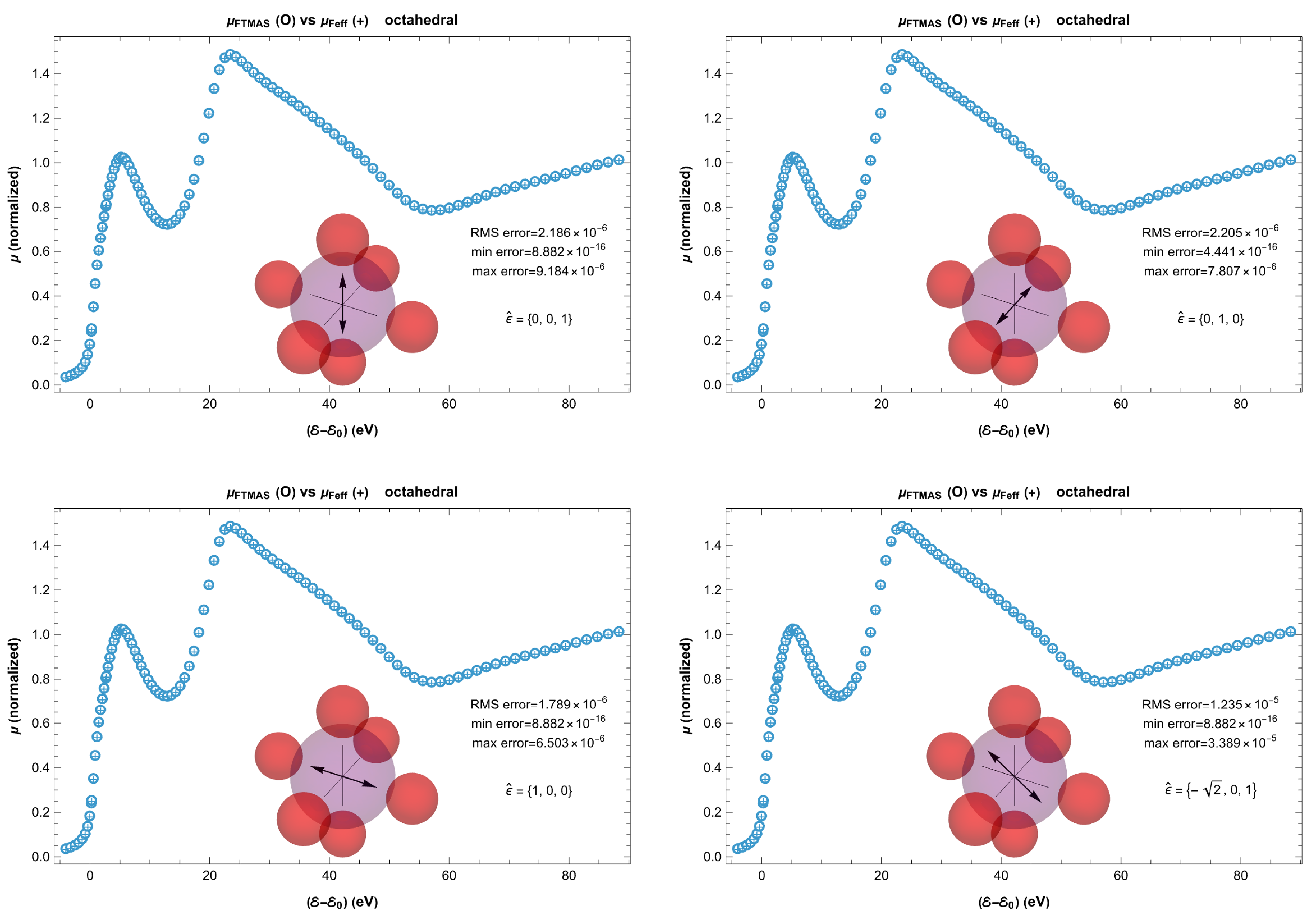
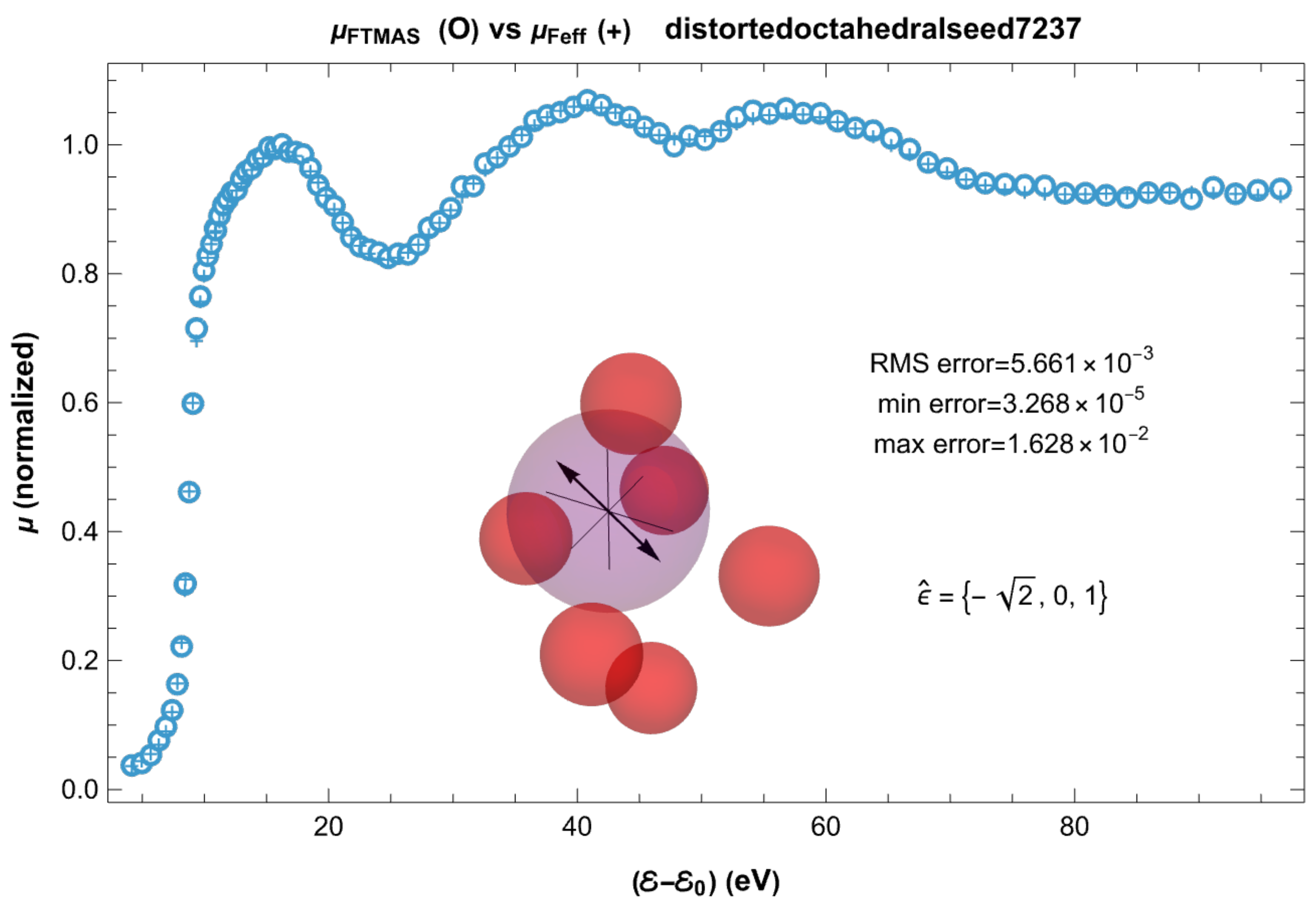
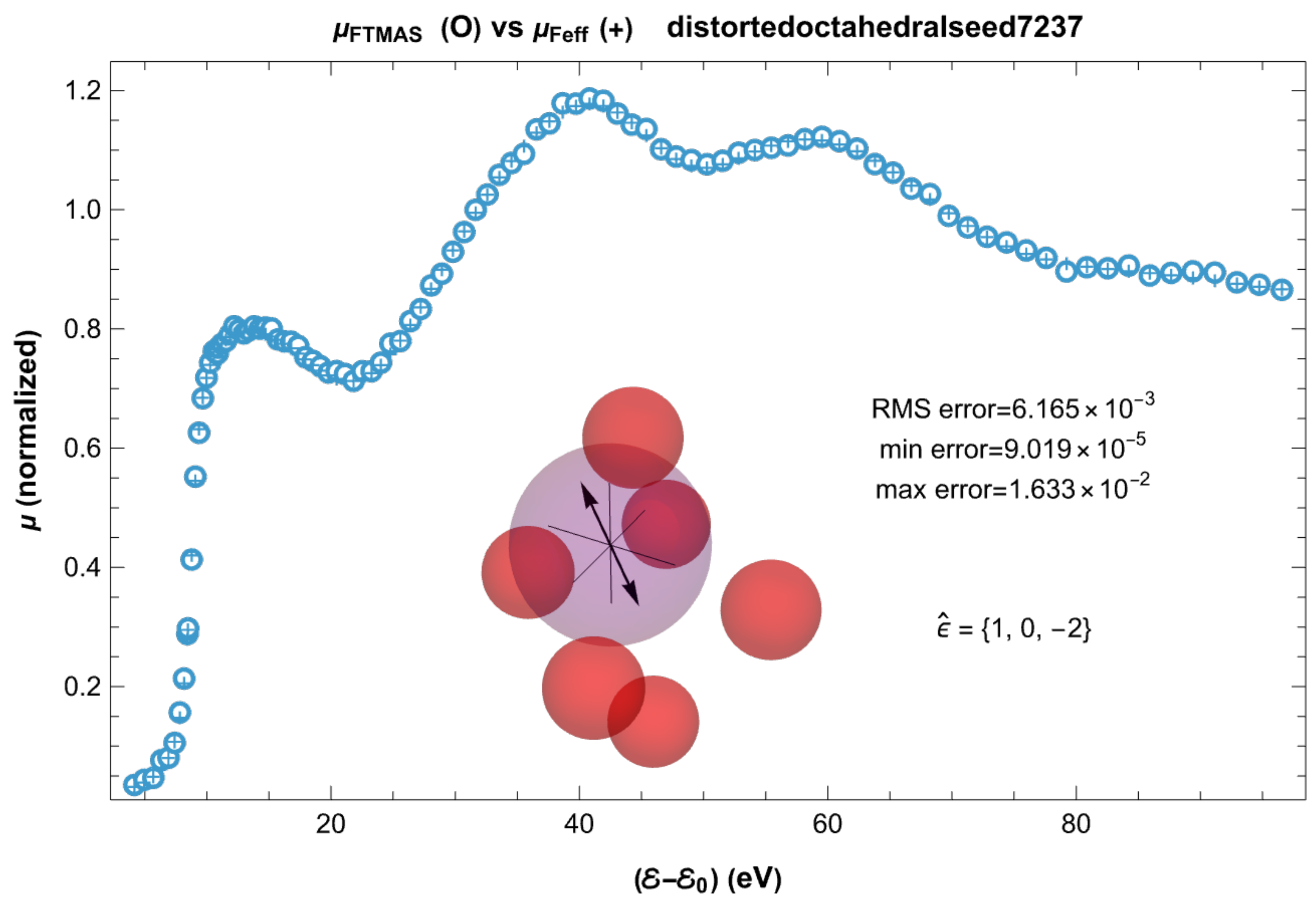
We find excellent agreement in all test cases between the spectra generated by projecting our reconstructed estimated tensor, and the independent direct calculations using FEFF. In the following plots, the + symbols are the FEFF-calculated benchmark values, and the open symbols are the spectra from our FTMAPS-reconstructed tensor. Once the tensor is calculated, calculating the spectra is virtually instantaneous, and very useful for interactive exploration.

Below, we present a series of plots, most corresponding to orientations of $\overrightarrow{ϵ}=(1,0,0),(0,1,0),(0,0,1),(-\sqrt{2},0,1)$. The choice of $(-\sqrt{2},0,1)$ corresponds to a polarization that is parallel to the planar sample surface, which is therefore inaccessible in practice to a direct absorption experiment. A key benefit of our approach is that the spectra for any orientations of $\overrightarrow{ϵ}$ can be instantly synthesized from the computed tensor, once it is constructed from the experimental data.

We start with our simplest structure: symmetric octahedral coordination. The coordinates (in Å) are given in

Table 5. Octahedral structure: positions of oxygen atoms in Å. Mn central atom is at (0, 0, 0).

	x	y	z
1	−2.	0.	0.
2	2.	0.	0.
3	0.	−2.	0.
4	0.	2.	0.
5	0.	0.	−2.
6	0.	0.	2.

, and results are shown in Figure 7. This is a cubic point group symmetry, and the absorption is observed to be independent of orientation. Here, only two orientations are shown; all others are identical.

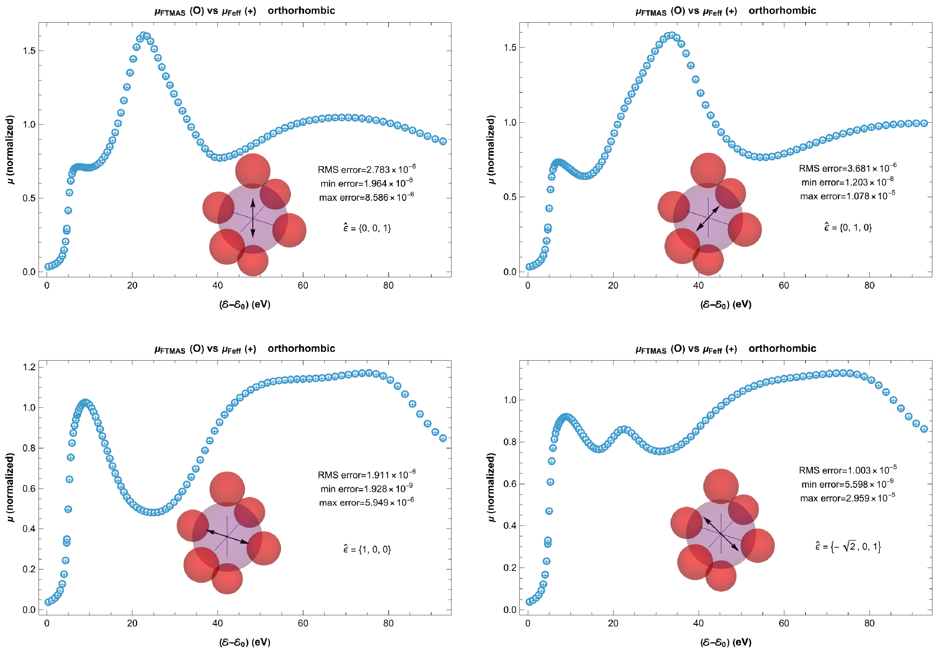
We then break the symmetry by an orthorhombic distortion, where distances in the x, y, z directions are different, but the angles are unchanged, and inversion symmetry is preserved. Coordinates are given in

Table 6. Orthorhombically distorted octahedral structure: positions of oxygen atoms in Å. Mn central atom is at (0, 0, 0).

	x	y	z
1	−1.6	0.	0.
2	1.6	0.	0.
3	0.	−2.	0.
4	0.	2.	0.
5	0.	0.	−2.2
6	0.	0.	2.2

, and results are shown in Figure 8.

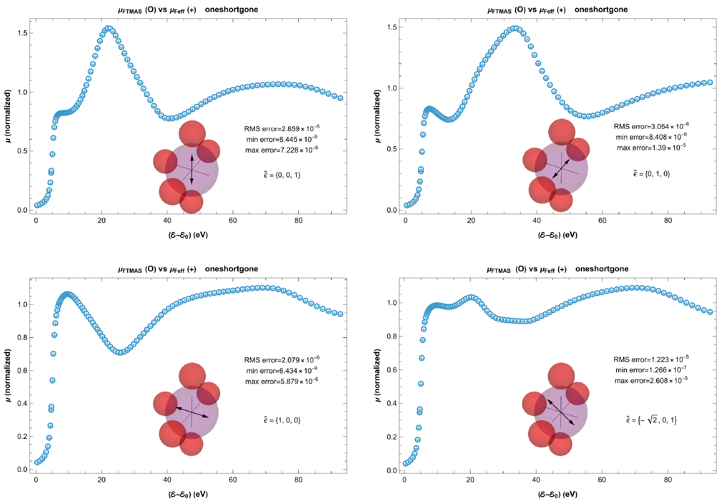
We then remove one of the short bonds to leave a 5-coordinate structure. This breaks inversion symmetry in the x-direction. Coordinates are given in

Table 7. The 5-coordinate structure, distorted octahedral, missing one short-distance atom; positions of oxygen atoms in Å. Mn central atom is at (0, 0, 0).

	x	y	z
1	−1.6	0.	0.
2	0.	−2.	0.
3	0.	2.	0.
4	0.	0.	−2.2
5	0.	0.	2.2

, and results are shown in Figure 9.

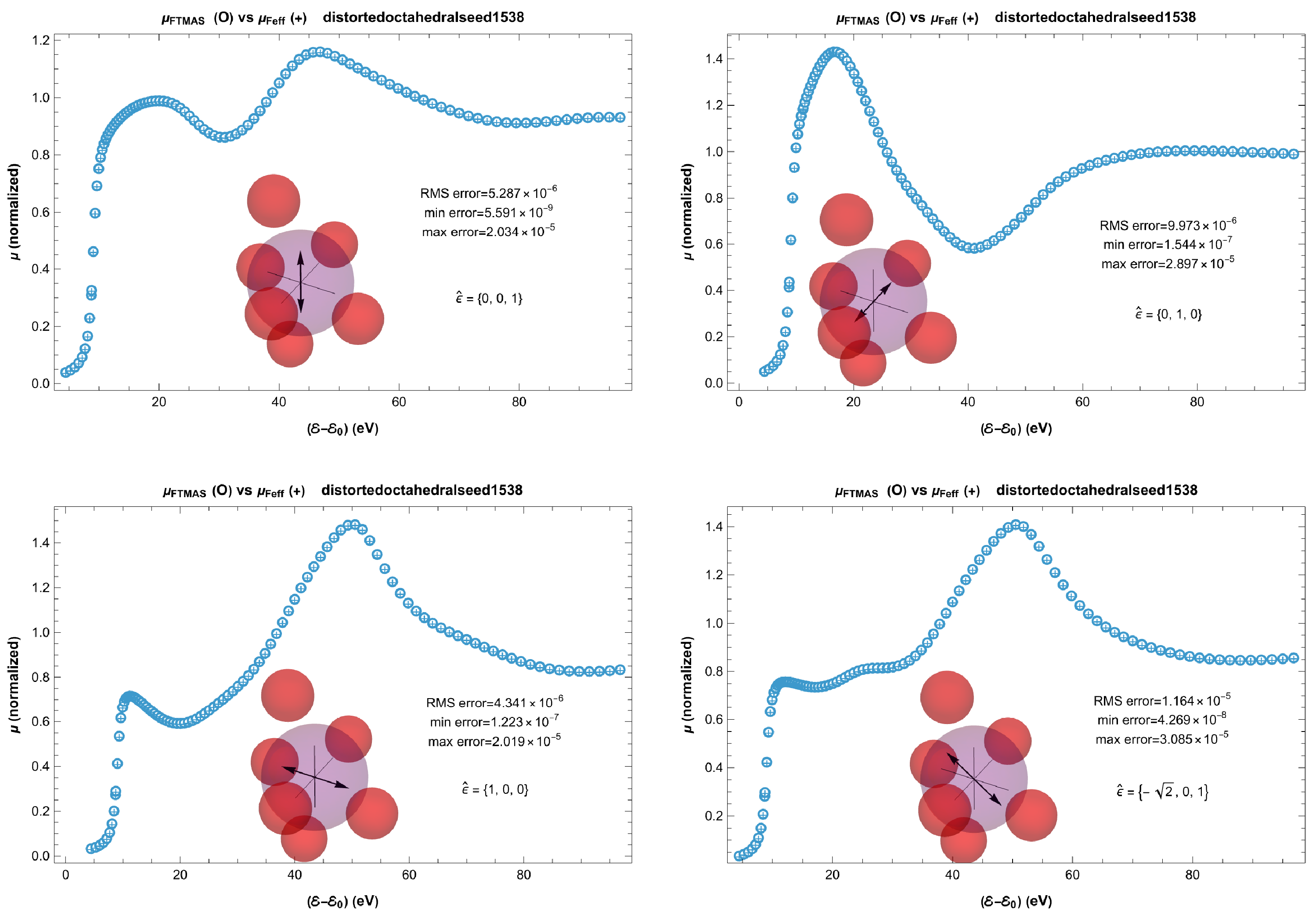
We then restore the 6-coordinate structure, but perturb the positions of each atom pseudo-randomly in x, y, z to break all point group symmetries. For reproducibility, a random seed (1538) is used; two examples are shown. Coordinates are given in

Table 8. Randomly distorted octahedral structure seed 1538: positions of oxygen atoms in Å. Mn central atom is at (0, 0, 0).

	x	y	z
1	−1.55068	0.527984	−0.367743
2	1.72223	−0.122876	−0.452528
3	−0.0555927	−1.39499	−0.0722204
4	−0.119001	2.1574	−0.116661
5	−0.519078	0.286155	−2.52098
6	−0.759075	0.031063	2.22597

, and results are shown in Figure 10.

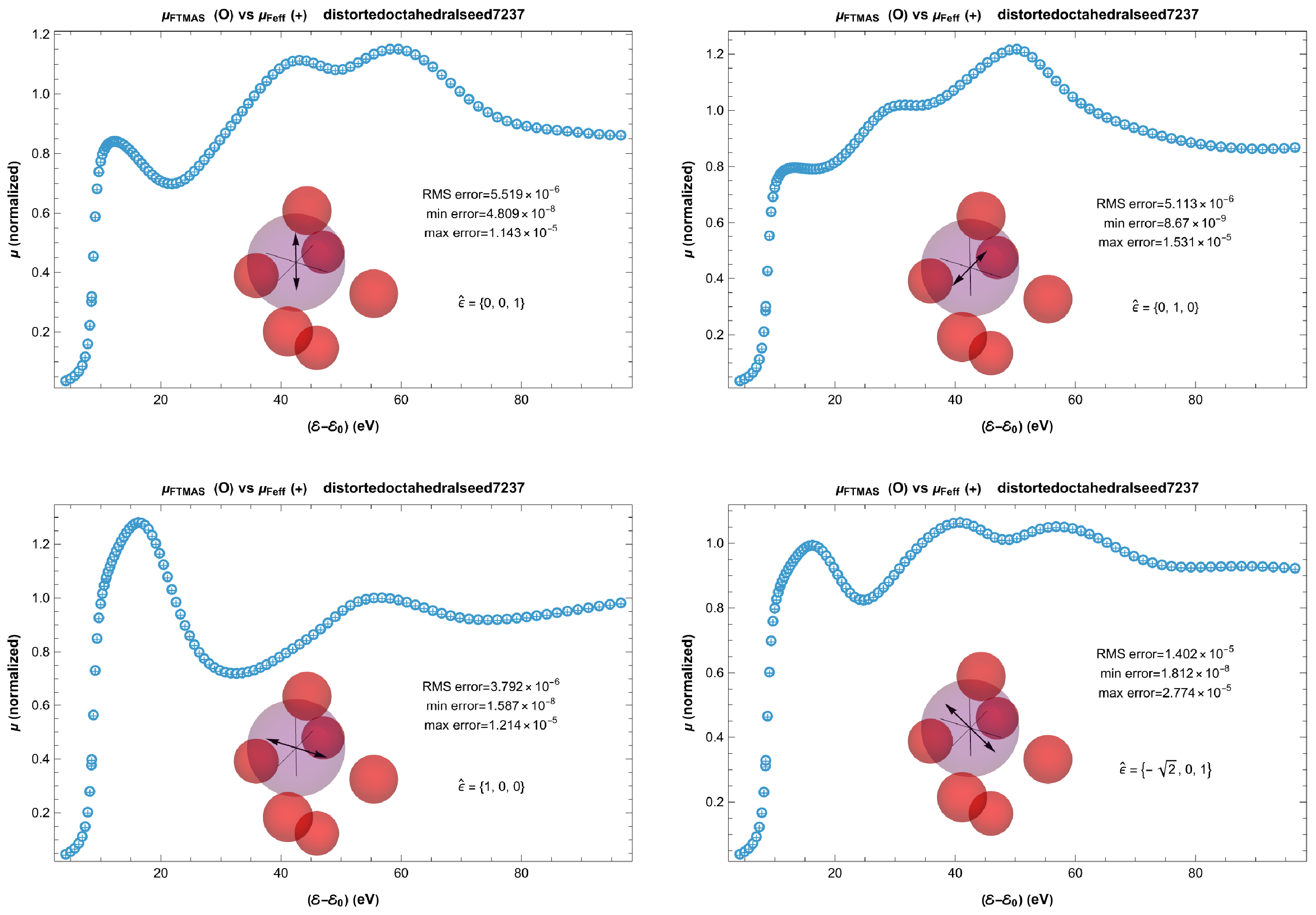
A different randomly generated structure with random seed 7237 is also shown, with coordinates in

Table 9. Randomly distorted octahedral structure seed 7237: positions of oxygen atoms in Å. Mn central atom is at (0, 0, 0).

	x	y	z
1	−1.20005	−0.265138	−0.701422
2	2.44578	−0.0605209	−0.192191
3	0.886845	−2.01818	−0.703688
4	−0.0168214	1.68493	−0.648975
5	0.860387	−0.344029	−2.58307
6	0.277901	0.151987	1.68977

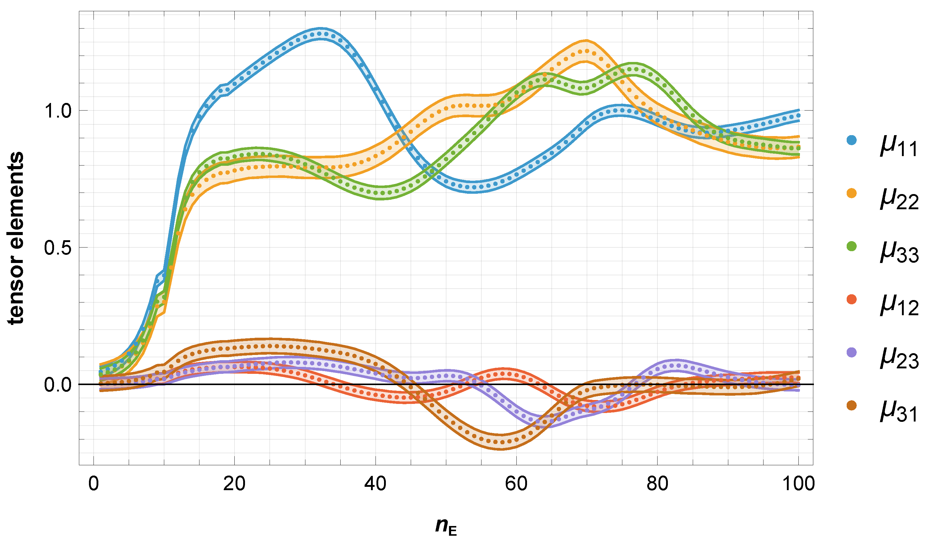
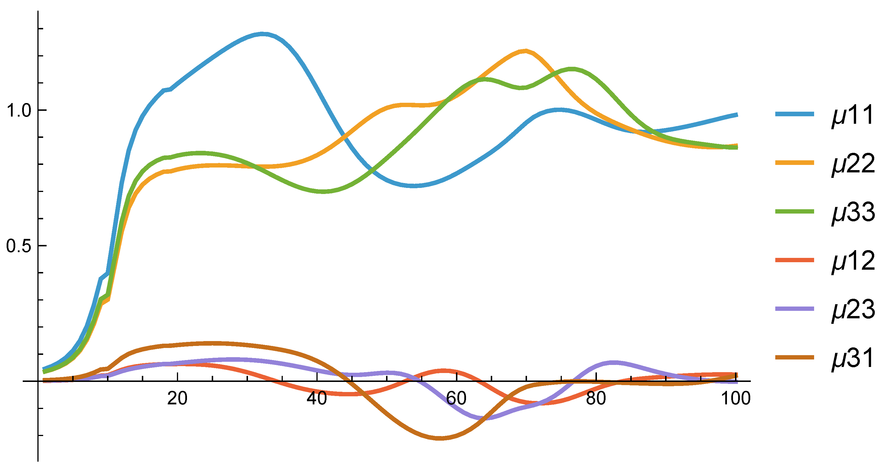
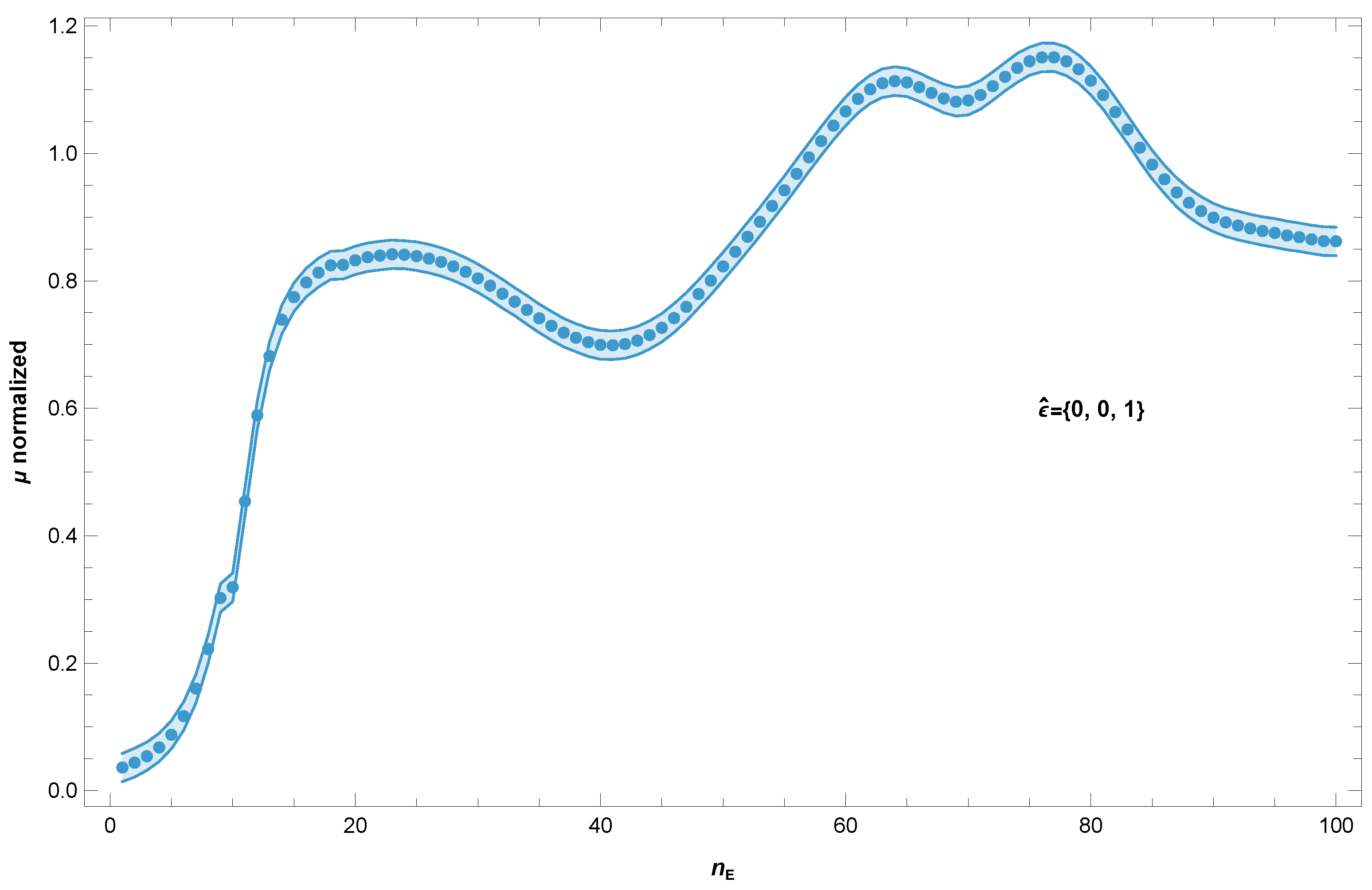
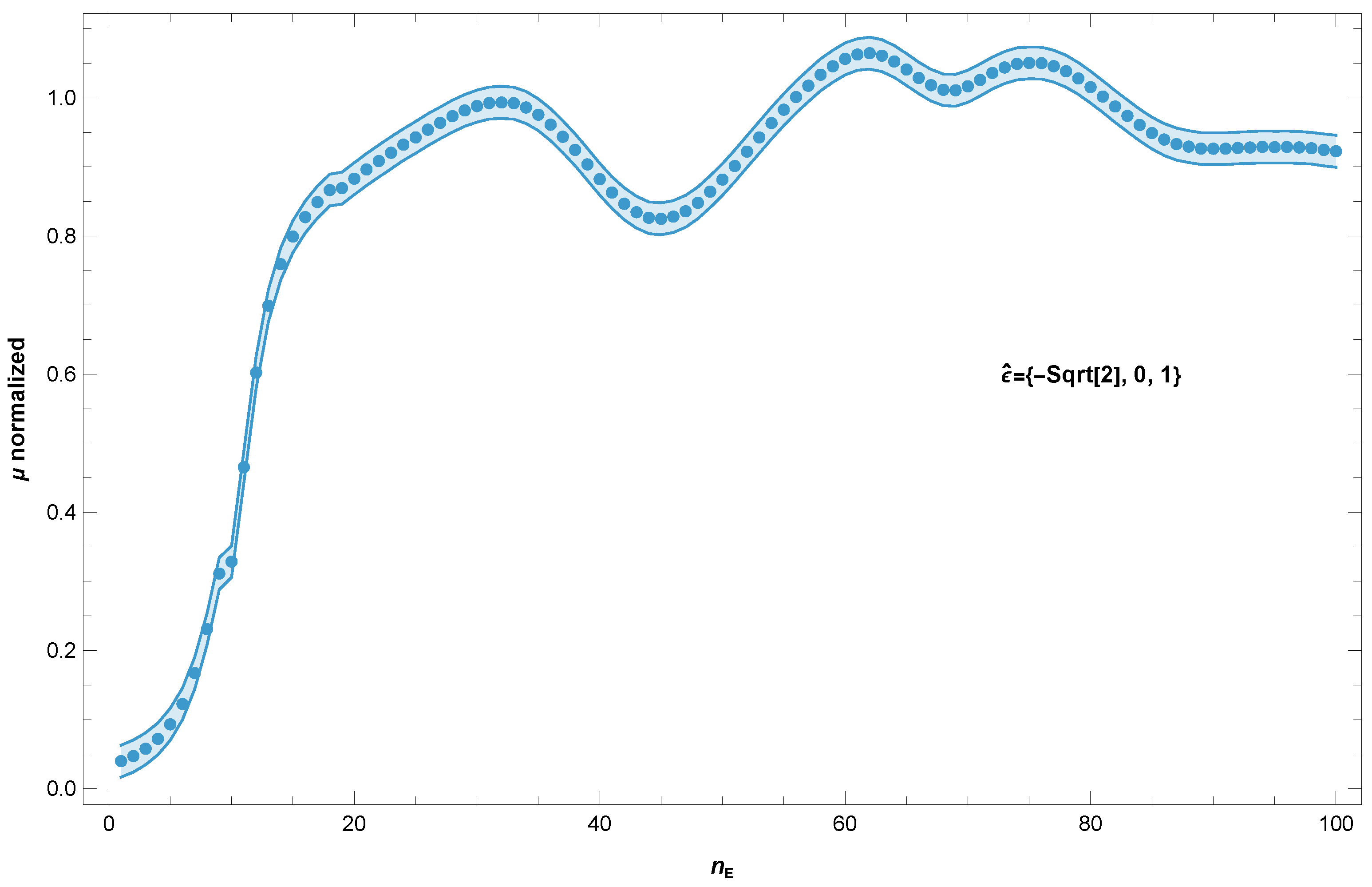
, and results are shown in Figure 11. The tensor elements vs. energy are shown in Figure 12.

It can be seen that the reconstructed spectra in all cases are in excellent agreement with the benchmark FEFF calculations, illustrating the accuracy of the reconstructed tensor. The resulting RMS, minimum, and maximum mismatch residual are shown on all plots.

3.2. Noisy Data

To illustrate the robustness of this procedure with something like real-world noisy spectra, we added synthetic randomly generated noise (uniformly distributed between $\pm 0.05$) to each of the spectral points for all angles and energies (i.e., 6000 random numbers) in the last example, and processed it identically to the other data sets. This noise analysis is extended significantly in the next subsection’s Monte Carlo calculations. This $\pm 5\%$ noise level (edge steps are $\approx 1$) is considerably larger than what should be expected from experimental data, but even in such a case the tensor reconstruction is robust, as shown in Figure 13. The visible noise level shown simply reflects the added spectral noise, and no systematic shift from the FEFF-calculated reference value is seen. The RMS, minimum, and maximum deviations from the noise-free FEFF calculations are shown on each plot. The determined variations are considerably less than $0.05$ for the following reason: the tensor elements are entirely derived from the basis functions (1, $cos\left(\alpha \right)$, $sin\left(\alpha \right)$, $cos\left(2\alpha \right)$, $sin\left(2\alpha \right)$), which have a limited bandwidth, while the noise also has higher-frequency components in it. The process of projecting onto this limited set of low-frequency basis functions (which are complete for our purposes) makes irrelevant those high-frequency components, reducing the noise in the reconstructed data. Similarly, any frequency components higher than $2\alpha$ are orthogonal and automatically filtered out by the projection. The overall robustness is a direct consequence of this Fourier decomposition, plus the well-conditioned PseudoInverse matrix in Table 4, which depends in part on our choice of the second angle ${\theta }_c$.

Another example is given in Figure 14. This is a different projection than the previous ones because it shows other structures (exposed using Manipulate to explore spectrum vs. orientation). The reconstructed projected tensor again agrees well with the FEFF calculation at that orientation, modulo the added noise.

This indicates the Fourier decomposition and oversampling in angle worked well. This makes sense since the reconstruction fundamentally relies solely on a sufficiently accurate determination of the Fourier coefficients of the angular behavior. Each energy value is independent of the others. Sampling at 60 different angular values spreads much of the added noise spectrum outside the frequency range that is used for the reconstruction process, so that it does not alias to the lower angular frequencies that are used in the Fourier decomposition.

Note that, in our pseudo-inverse implementation, the Fourier decomposition and the full-tensor reconstruction are both expressible simply by matrix multiplications by constant-valued, low-dimensional matrices (Table 4 and Table 5). In fact, these can be combined into a single exact matrix (in the current example, dimension $6\times 120$) that transforms a 120-element array consisting of concatenated arrays of spectra for a fixed energy (60 angles each for ${\theta }_m$ and ${\theta }_c$), and maps it directly to the 6 unique tensor elements. This matrix multiplication is then done for each energy slice. The process is very simple, direct, robust, and exact (infinite precision): all elements of the resulting matrix are integers, rationals, $\pi$, and square roots thereof, in our implementation; machine precision (64 bit) floating point is quite sufficient for this purpose.

3.3. Monte Carlo Calculations

The examples above illustrate the accuracy of the reconstruction with respect to the benchmark reference FEFF calculations, and also tolerance for noise, but only for individual random instances, drawn from a uniform distribution.

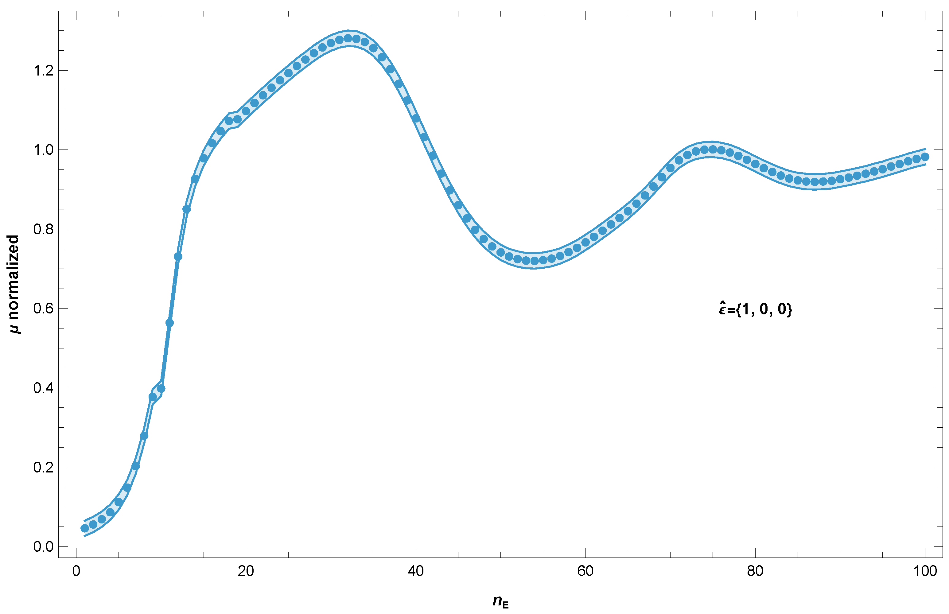
Here, we show with much greater statistical sampling weight, using a normal distribution, calculations of the tensor elements with standard deviations, and also spectra corresponding to different projections of the reconstructed tensors, each averaged over ${10}^4$ randomly perturbed spectra for each data point, ${10}^4$ random tensors calculated for each of the 100 energy points.

Normally distributed random variates, of zero mean and standard deviation $0.1$, were added to each of the 120 $\alpha$ samples (60 each for ${\theta }_m$ and ${\theta }_c$), and the corresponding noisy tensor elements were calculated by matrix multiplication as described above. For each energy, this was repeated (with different random variates) ${10}^4$ times, and the mean and standard deviation of all tensor elements were calculated. This process was then repeated for each of the 100 energy slices. 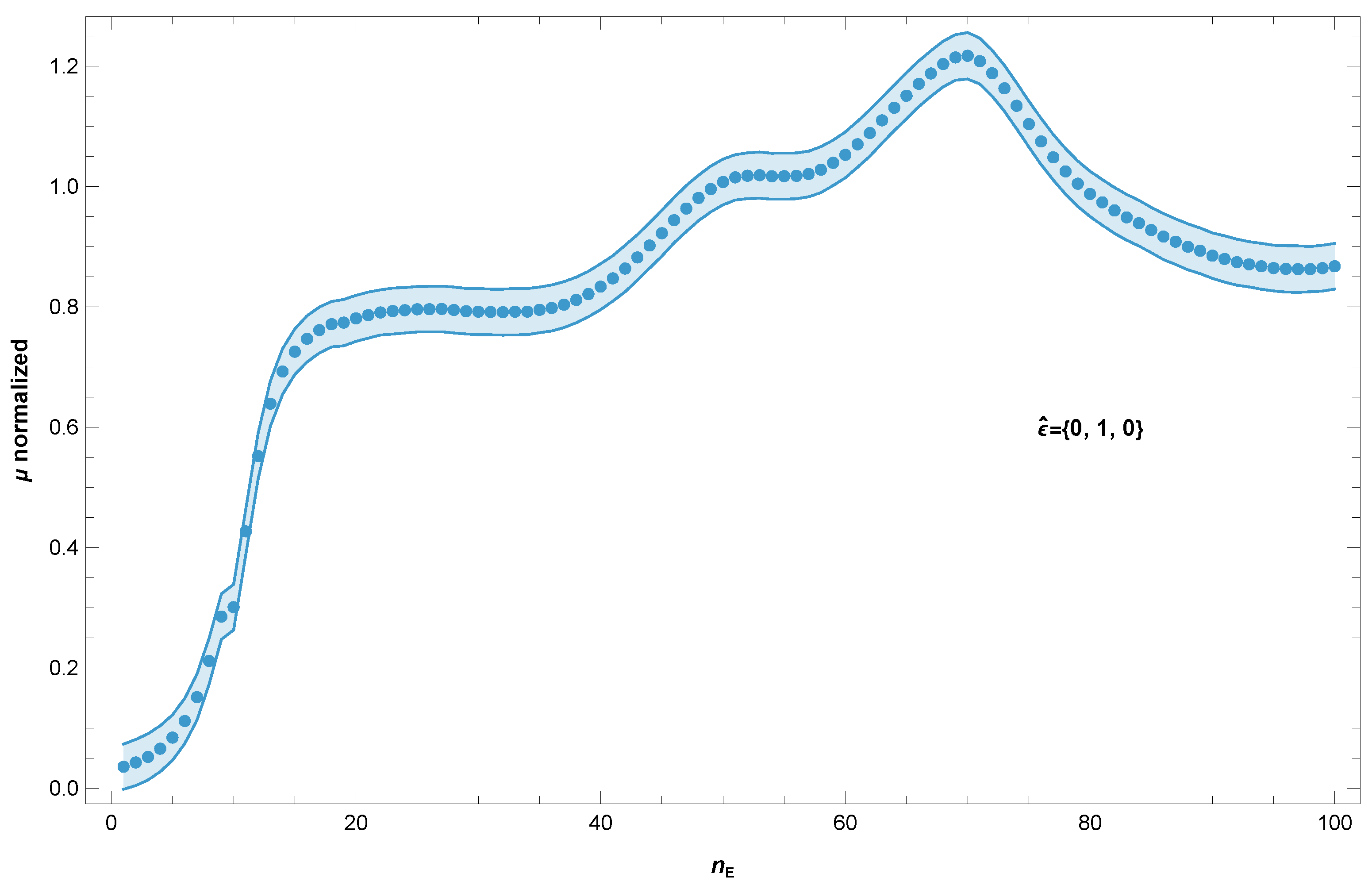To be quite clear, this involves the generation of $120\times {10}^4\times 100=120$ million normally distributed random variates. The tensor elements with corresponding error bars are plotted in Figure 15, and the tensors are then projected onto the polarization directions. The standard deviations of the projected spectra are also displayed as error bands about the mean values. The zero-noise spectra are also over-plotted, but these are essentially identical to the mean-value spectra.

3.4. Plots of Projected Spectra with Error Bands

Monte Carlo averages of projected spectra, with one-$\sigma$ uncertainties are shown in Figure 16, Figure 17, Figure 18 and Figure 19.

3.5. Explicit Tensors with Errors

Here, we further give 20 explicit reconstructed tensors with standard deviations of the elements at a range of energies for every fifth energy grid point from $n_E=5$–100. The energy grid is the same as shown in Figure 13. One third of the sum of the diagonal elements is the 3D isotropic average, i.e., the sought-after XAFS spectrum. The random deviates and calculations are as described above in this subsection.

Explicit tensor elements with standard deviations at a representative subset of the 100 energies are shown in

Table 10. Explicit reconstructed tensors at energy indices ($10,20$) (top left and right); similarly for ($30,40$), ($50,60$), ($70,80$), ($90,100$). Only a limited set of the 100 total is shown to conserve space. Noise is drawn from normal distribution with $\sigma =0.1$, i.e., $1/10$ of the edge step. To obtain high accuracy of the off-diagonal elements well above the edge, low-noise data can be obtained by usual methods.

$\begin{array}{c}\left(\begin{array}{ccc}0.398\pm 0.019& 0.022\pm 0.019& 0.046\pm 0.026\\ 0.022\pm 0.019& 0.30\pm 0.04& 0.020\pm 0.020\\ 0.046\pm 0.026& 0.020\pm 0.020& 0.319\pm 0.022\end{array}\right)\end{array}$	$\begin{array}{c}\left(\begin{array}{ccc}1.097\pm 0.019& 0.063\pm 0.019& 0.134\pm 0.026\\ 0.063\pm 0.019& 0.78\pm 0.04& 0.067\pm 0.020\\ 0.134\pm 0.026& 0.067\pm 0.020& 0.832\pm 0.022\end{array}\right)\end{array}$
$\begin{array}{c}\left(\begin{array}{ccc}1.269\pm 0.020& 0.033\pm 0.019& 0.133\pm 0.026\\ 0.033\pm 0.019& 0.79\pm 0.04& 0.079\pm 0.020\\ 0.133\pm 0.026& 0.079\pm 0.020& 0.804\pm 0.022\end{array}\right)\end{array}$	$\begin{array}{c}\left(\begin{array}{ccc}1.079\pm 0.019& -0.038\pm 0.019& 0.074\pm 0.026\\ -0.038\pm 0.019& 0.83\pm 0.04& 0.040\pm 0.020\\ 0.074\pm 0.026& 0.040\pm 0.020& 0.700\pm 0.023\end{array}\right)\end{array}$
$\begin{array}{c}\left(\begin{array}{ccc}0.741\pm 0.019& -0.027\pm 0.019& -0.120\pm 0.026\\ -0.027\pm 0.019& 1.01\pm 0.04& 0.032\pm 0.020\\ -0.120\pm 0.026& 0.032\pm 0.020& 0.823\pm 0.022\end{array}\right)\end{array}$	$\begin{array}{c}\left(\begin{array}{ccc}0.766\pm 0.019& 0.034\pm 0.019& -0.202\pm 0.027\\ 0.034\pm 0.019& 1.05\pm 0.04& -0.099\pm 0.020\\ -0.202\pm 0.027& -0.099\pm 0.020& 1.066\pm 0.023\end{array}\right)\end{array}$
$\begin{array}{c}\left(\begin{array}{ccc}0.954\pm 0.019& -0.078\pm 0.019& -0.021\pm 0.027\\ -0.078\pm 0.019& 1.22\pm 0.04& -0.095\pm 0.020\\ -0.021\pm 0.027& -0.095\pm 0.020& 1.083\pm 0.023\end{array}\right)\end{array}$	$\begin{array}{c}\left(\begin{array}{ccc}0.964\pm 0.019& -0.027\pm 0.019& -0.001\pm 0.026\\ -0.027\pm 0.019& 0.99\pm 0.04& 0.056\pm 0.020\\ -0.001\pm 0.026& 0.056\pm 0.020& 1.114\pm 0.022\end{array}\right)\end{array}$
$\begin{array}{c}\left(\begin{array}{ccc}0.926\pm 0.019& 0.017\pm 0.019& -0.010\pm 0.026\\ 0.017\pm 0.019& 0.89\pm 0.04& 0.026\pm 0.020\\ -0.010\pm 0.026& 0.026\pm 0.020& 0.899\pm 0.022\end{array}\right)\end{array}$	$\begin{array}{c}\left(\begin{array}{ccc}0.982\pm 0.020& 0.024\pm 0.019& 0.021\pm 0.026\\ 0.024\pm 0.019& 0.87\pm 0.04& -0.002\pm 0.020\\ 0.021\pm 0.026& -0.002\pm 0.020& 0.862\pm 0.022\end{array}\right)\end{array}$

.

3.6. Systematic Errors

We consider three types of systematic error “injected” at the Fourier coefficient level. Each of these spurious influences should be minimized by careful attention to the experiment. These examples serve to illustrate the size of the effect, which can be simply and precisely calculated using the matrices above.

For illustration, the first is an example of a large error of a $10\%$ linear gradient in sample thickness over the sample, as was explicitly calculated above. This adds a spurious sinusoidal component into the reconstruction. Explicit tensors evaluated at the 25th energy grid point are shown below in

Table 11. A $10\%$ linear gradient error: left tensor unperturbed, right tensor is perturbed.

$$\left(\begin{array}{ccc}1.19303& 0.05792& 0.139927\\ 0.05792& 0.79618& 0.077798\\ 0.139927& 0.077798& 0.838856\end{array}\right),\left(\begin{array}{ccc}1.19381& 0.0353754& 0.141925\\ 0.0353754& 0.783193& 0.029361\\ 0.141925& 0.029361& 0.839355\end{array}\right)$$

, for the unperturbed (left) and perturbed (right) cases.

The second example is of a large $5\%$ differential normalization error between measurements at ${\theta }_m$ and ${\theta }_c$. This multiplies the signals for ${\theta }_m$ by $1.05$ while leaving that for ${\theta }_c$ unchanged. Explicit tensors evaluated at the 25th energy grid point (see Figure 15) are shown below in

Table 12. A $5\%$ differential normalization error: left tensor unperturbed, right tensor is perturbed.

$$\left(\begin{array}{ccc}1.19303& 0.05792& 0.139927\\ 0.05792& 0.79618& 0.077798\\ 0.139927& 0.077798& 0.838856\end{array}\right),\left(\begin{array}{ccc}1.21779& 0.0587023& 0.11141\\ 0.0587023& 0.855126& 0.0805317\\ 0.11141& 0.0805317& 0.854566\end{array}\right)$$

, for the unperturbed (left) and perturbed (right) cases.

The third example is of a large 6-degree differential error in the zero angle of $\alpha$ between the measurements at ${\theta }_m$ and ${\theta }_c$. Here, we implement it by cyclically shifting the measurements vs. angle for ${\theta }_m$ by one position ($360/60=6$ degrees) while leaving that for ${\theta }_c$ unchanged. Explicit tensors evaluated at the 25th energy grid point are shown below in

Table 13. Six-degree differential phase angle error: left tensor unperturbed, right tensor is perturbed.

$\left(\begin{array}{ccc}1.19303& 0.05792& 0.139927\\ 0.05792& 0.79618& 0.077798\\ 0.139927& 0.077798& 0.838856\end{array}\right),\left(\begin{array}{ccc}1.18806& 0.0693218& 0.13205\\ 0.0693218& 0.803173& 0.0826091\\ 0.13205& 0.0826091& 0.845399\end{array}\right)$

, for the unperturbed (left) and perturbed (right) cases.

We conclude that such systematic perturbations (which should be minimized much below this level by experimental technique), even when“injected” at the Fourier coefficient level, have effects on the reconstructed tensor elements that are only of the same order as the perturbations, as mathematically proven above. The method is quite robust, and we emphasize that such calculations of reconstruction errors and noise are quite simple and direct using the given matrices.

4. Discussion

Our results indicate that full-tensor magic angle pair spectroscopy (FTMAPS) may potentially become a promising experimental modality for determining the full dipole optical absorption tensor in near-real-time. It is a nontrivial extension of conventional magic angle spinning (whence the name FTMAPS). Conventional magic angle spinning provides only the trace (sum of diagonal elements) of the tensor at each energy, not all six unique elements. An example plot of all six unique tensor elements vs. energy is shown in Figure 12. In this case, all elements are nonzero because of the low symmetry. For the octahedral case (any cubic symmetry, including tetrahedral), only the diagonal elements are nonzero, and they are all equal. In the orthorhombic case all off-diagonal elements are zero, but the three diagonal entries are different from each other. FTMAPS scans can immediately provide such information about the underlying symmetry of the absorbing site.

It is generally recognized that incisive information can be obtained by linear dichroism. In XAFS (“polarized XAFS”), it is occasionally used to obtain specific information (e.g., absorption parallel and perpendicular to a surface on which an atom is adsorbed). Only rarely is it used to obtain the full-tensor elements, owing to the difficult and time-consuming nature of the angular scans, or prior information about the structure that are required to perform the measurements, as well as the complexity of interpreting the measured spectra.

As we have shown above, an important use of the full-tensor information is to permit the fast calculation of the spectra for any chosen orientation, even those that are experimentally inaccessible. This allows one (in a sense) to “look along” certain directions. The full tensor spectrum calculated this way then can be analyzed in the standard manner: in the case of XAFS, to investigate spectral features (e.g., focusing multiple scattering paths, or to emphasize contributions from a particular ligand of interest) whose signals tend to be averaged out in the usual isotropically averaged spectrum. As can be seen in the examples given above, information about nearest-neighbor interatomic distances can be inferred from edge shifts that depend on the orientation of the polarization vector. Using theoretical calculations to fit hypothetical model structures to the experimental full tensor data might be used to fully determine the local structure of the site. The predictions using the dipole tensor may also help to identify deviations from pure dipole behavior, for example, quadrupole transitions. The full (Cartesian) tensor spectrum can also be used to decompose into alternative representations such as spherical tensors, if desired. Analyzing the eigenvalues and eigenvectors of the tensor gives information about the orientation of the site as a function of energy.

It is the experimental and analytical simplicity of FTMAPS that shows particular promise relative to conventional methods. It is true that its application appears to be limited to samples with a flat surface; a homogeneous thin film sample of uniform thickness is ideal. Many samples are of this nature, or can be made this way, however, and having a uniform-thickness film obviates a whole class of experimental nuisances in conventional methods that arise from the changing effective thickness presented to the beam as it is rotated. In FTMAPS, this is not a concern. Differences in absorption length between spectra at ${\theta }_m$ and ${\theta }_c$ are trivially calculable and correctable.

No four-circle goniometry is required, only a sample spinner whose axis is set to two discrete fixed positions: the magic angle and its complement. Simple measurements could even be done with essentially no additional instrumentation, albeit more slowly, by doing energy scans with the spin angle set to a sequence of discrete equally spaced values. Angle changes could even be done manually between groups of energy scans, or better, using a stepper motor and rotation stage. It seems likely, however, that spinning the sample continuously could be done more quickly and accurately, essentially by modulating at the spin frequency.

There are many ways to interface such an experiment with XAFS beamline data acquisition software, ranging in cost from a few dollars in parts for demodulator/ring counter ICs, or analog multiplier ICs, to several-hundred-dollar FPGA software virtual instruments, to as much one would like to pay. The best choices would depend on specifics of beamlines, their software, and preferences of beamline personnel. At its root, all that is necessary is to place the measured signals corresponding to particular spin angles and energy ranges into distinct counting bins. Inexpensive microcontrollers and integrated circuits chips can easily route the appropriate signals to different scaler channels. Alternatively, either analog circuits or digital or microcontrollers could be used to directly compute the five Fourier components as a function of time, to produce signals for readout by the beamline data acquisition system. As shown above, this would just involve taking five dot products with fixed numerical arrays. The bandwidth requirements are minimal because the modulation frequency is the spin frequency, which is likely in the low audio range.

As noted above, once the data are acquired vs. energy and spin angle $\alpha$ (at ${\theta }_m$ and ${\theta }_c$), the full data conversion from spectra to the tensor elements can be done using only a single matrix multiplication. This operation would be done at each energy point. We find that using the exact, symbolic matrix (for 60 angle samples) takes about one millisecond on the author’s laptop computer, so a full energy spectrum is less than a second. Doing it numerically at machine precision is about a thousand times faster. It could easily be automatically performed at a beamline to aid in interpreting the data.

Although we here have discussed the application of the FTMAPS to X-ray Absorption Fine Structure spectra, the fundamental dipole tensor character potentially renders it broadly applicable to longer wavelengths of light, such as UV–Vis, IR, THz, or microwave, provided the absorbing components are small in dimension compared to the wavelength. The same basic logic and mathematics of data to tensor mapping are the same. As in XAFS applications, FTMAPS for other wavelengths does require a flat sample surface, but many samples already have this character, or can be made so. Given the importance of thin films in science and industry, for many purposes, e.g., semiconductors and perovskite photovoltaics, it may find application in material characterization and process control. Applications to biochemical adsorbed films in science and diagnostics is also an obvious potential application.

FTMAPS can provide information that is otherwise experimentally inaccessible—such as absorption spectra measured along any direction parallel to the sample surface—and by doing measurements that are relatively fast and easy. FTMAPS has the potential to provide up to six times the information that is normally available in isotropically averaged experiments, and can make full-tensor measurements far more easily than laborious angle measurements using four-circle goniometry, which also has its own systematic errors.

We have shown above that even rather noisy data are handled robustly by this approach: it mostly relies on the accurate Fourier decomposition of the angular dependence, at relatively low frequencies; transformation from Fourier coefficients to tensor elements is stable and robust. This can be ensured by oversampling an angle to reject spurious noise components, or by analog filtering before sampling. The two steps—conversion from spectra to Fourier coefficients, and conversion from Fourier coefficients to tensor elements—can be combined into one simple matrix multiplication.

As stated above, the scope and purpose of this paper is to explain the concept, theory, and data reduction process, and to demonstrate that it works using synthetic data with added noise. A full treatment of experimental implementation is deferred for later work and papers. Nevertheless, here, we briefly address some experimental considerations and some remedies/preventions.

Gradients in sample thickness can be diagnosed simply by repeating measurements with the sample remounted at a quarter turn. The errors introduced by such imperfections are discussed below. The misalignment of the sample surface normal and spin axis can be checked using a machinist’s dial indicator, or by mounting a mirror and monitoring a reflected light beam as it rotates. Samples of known cubic crystal symmetry (an angular blank) can be measured to test that there is no spurious angular signal owing to various mechanical imperfections. The modulation (spin) frequency should be chosen to avoid ambient EMF noise sources, and to be compatible with time constants (e.g., current amplifiers, ionization chambers) in the data acquisition system. Shifts in sample position when changing between ${\theta }_c$ and ${\theta }_m$ measurements can be made negligible using appropriate mechanical design; quadrature encoders on the spin-axis rotary shaft can be used to accurately determine angles and to standardize angle zeros for the two orientations.

As a slightly less trivial example, making use of equations in Table 1 (or similarly for Table 2), we briefly analyze the effect of a small gradient in sample thickness. An ideal sample should be uniform in thickness, but of course some nonzero variation is inevitable. A linear gradient in absorption would amplitude-modulate the spin-angle dependence by a factor of $1+ϵcos(\alpha +\delta )$, where $ϵ$ is the relative size of the linear gradient and $\delta$ describes the orientation of the gradient with respect to the zero of $\alpha$. The additional cosine and sine factors add contributions at frequencies higher and lower than the basis function of interest.

It is not difficult to show using trig formulae that the $ϵcos(\alpha +\delta )$ multiplicative factor induces errors in the estimated fourier coefficients $b_1\dots b_5$ of the basis functions $(1,cos\left(\alpha \right),sin\left(\alpha \right),cos\left(2\alpha \right),sin\left(2\alpha \right))$:

$$\begin{array}{c}\Delta b_1={\displaystyle \frac{1}{2}}ϵ(b_{2}cos\left(\delta \right)-b_{3}sin\left(\delta \right))\\ \Delta b_2={\displaystyle \frac{1}{2}}ϵ((2b_1+b_4)cos\left(\delta \right)-b_{5}sin\left(\delta \right))\\ \Delta b_3={\displaystyle \frac{1}{2}}ϵ(b_{5}cos\left(\delta \right)+(b_4-2b_1)sin\left(\delta \right))\\ \Delta b_4={\displaystyle \frac{1}{2}}ϵ(b_{2}cos\left(\delta \right)+b_{3}sin\left(\delta \right))\\ \Delta b_5={\displaystyle \frac{1}{2}}ϵ(b_{3}cos\left(\delta \right)-b_{2}sin\left(\delta \right))\end{array}$$

The essential feature we wish to stress is that all such systematic errors induced by the linear thickness gradient across the sample are of order $ϵ$, with coefficients of order 1 or less. Because of the structure of the pseudo-inverse matrix (Table 4), which maps Fourier coefficients to tensor elements, the changes in the estimated tensor elements are also of order $ϵ$ with coefficients of order 1 or less. A $1\%$ gradient gives a change to the tensor elements of that same scale. No instability or amplification of error is found.

Noise in the data affects the dependence of the absorption on spin angle, which affects the Fourier coefficients, which affect the computed tensor elements. As shown above, the effect of random noise is strongly moderated by the filtering effect of projecting the data onto the low-order Fourier components. Effectively, the Fourier decomposition is a low-pass filter (in angle) that reduces the noise level. The structure of the pseudo-inverse matrix given in Table 4 shows that this disturbance will not be amplified by that process. Each entry in the table is of order 1 or less, and the terms vary in sign. A noisy contribution of order ${ϵ}_n$ or less will produce an effect of the same order in the determined tensor elements.

The description we present here presumes that it is direct absorption measurements that are to be made. Fluorescence excitation spectra are also commonly used to measure XAFS, and these have similar dipolar character, to the extent the initial absorption is de-correlated with the subsequent emission. In many cases, this approach should work as well with fluorescence excitation spectra, but there are nuances in this comparison that need to be considered [6,21], and this will need to be tested. The more general photon-in/photon-out aspects of Resonant Inelastic X-ray Scattering are beyond the scope of the current paper.

5. Conclusions

We have proposed full-tensor magic angle pair spectroscopy (FTMAPS) as a simple and powerful potential experimental modality for measuring linear dichroic (polarized) X-ray Absorption (XAFS) spectra, and other optical (UV–Vis, IR, microwave, THz) spectra in the dipole approximation, to produce the full dipole tensor vs. energy (or wavelength). It is a relatively simple but nontrivial extension of conventional magic angle spinning in XAFS, but offers much of the same information more complex and time-consuming measurements requiring scanning using four-circle or kappa goniometers, and requires no previous knowledge about the microstructure (e.g., crystal symmetry) of the sample. Our conclusions in this paper, which describe the theory and data processing logic, and demonstrate its correctness, are based on a combination of theory and numerical simulations with virtual data, using FEFF as a benchmark. For full validation, experimental R&D and testing will be needed to turn it into a routinely used technique. For reasons of the scope and size of this paper, we defer a fuller description of experimental implementation to subsequent publications.

FTMAPS works by measuring the time (or spin angle) dependence of the optical (e.g., X-ray) absorption signal as a homogeneous planar film sample is rotated with its axis set at the magic angle $arctan\left(\sqrt{2}\right)=arccos\left({\displaystyle \frac{1}{\sqrt{3}}}\right)$ (and its complement) relative to the electric polarization vector of the linearly polarized photon beam. The magic angle is indeed special: if the spin axis makes this angle with respect to the X-ray polarization vector, uniformly averaging over the angle of rotation $\alpha$ about the spin axis gives a signal proportional to the 3D isotropic average spectrum, which is 1/3 of the invariant trace of the dipole absorption tensor.

For low-symmetry samples, the full dipole tensor signal offers up to six times more information (i.e., linearly independent spectra) than the usual isotropically averaged signal. In contrast, for samples with cubic symmetry, no additional information is provided: the signal is isotropic. Deviations from cubic symmetry should be readily apparent by FTMAPS, and often may be of interest, for example, in studying phase transitions or for industrial process control of films.

The examples given here are for X-ray Absorption Fine Structure (XAFS) spectroscopy using the linearly polarized beams from synchrotron radiation sources. The procedure is robust to noise in the data. When using continuous spinning, the DC and audio-frequency time dependence of the signal’s five Fourier components can be determined: a constant value (at each energy), corresponding to the isotropic signal that is normally sought and analyzed in XAFS measurements, plus coefficients of the sine and cosine components at the spin frequency, and twice that frequency. From the time (or angle) dependence, these components are straightforward to directly obtain from experimental data as a function of energy during a scan.

The full data reduction process, once understood, is remarkably simple. The $\mu$ spectra vs. spin angles are recorded for two discrete spin axis orientations ${\theta }_m$ and $thet{a}_c$, and their Fourier components (FCs) determined by matrix multiplication, or some other means. The FCs are the essential data needed to calculate the tensor elements, again by a simple matrix multiplication. If desired, the two matrices (spectra → FCs, and FCs to tensor elements) can be combined into a single spectra → tensor element transformation, which is repeated for each energy. This is stable and robust, and takes only milliseconds to compute. Once the tensor elements are determined at each energy, the spectra for polarizations with any orientation can be instantly computed, and more elaborate theoretical modeling, fitting, and analysis can be done. The whole data reduction process is direct, requires no additional input parameters, and takes about about one second to compute on a laptop computer.

In our initial implementation described here, the angles between the spin axis and the X-ray polarization vector are chosen to be the magic angle ${\theta }_m=arccos\left({\displaystyle \frac{1}{\sqrt{3}}}\right)=arctan\left(\sqrt{2}\right)$, and its complement ${\theta }_c={\displaystyle \frac{\pi }{2}}-{\theta }_m=arcsin\left({\displaystyle \frac{1}{\sqrt{3}}}\right)=arctan\left({\displaystyle \frac{1}{\sqrt{2}}}\right)$. In the geometry considered here, with the spin axes in the plane of the beam direction $\overrightarrow{k}$ and the polarization vector $\overrightarrow{ϵ}$, these two angles symmetrically straddle the ${45}^{\circ }$ degree orientation that is commonly used in fluorescence measurements.

Simple analytical equations are given to relate these numerical values to linear combinations of the tensor elements, resulting in a linear system that can be solved for the tensor elements at each energy. For the general case, with no assumed sample symmetry, six real numbers are required to specify all components of a symmetric Cartesian tensor in 3D. The sixth value, plus four others, can be obtained by measuring with a second spin axis, providing ten numbers per energy produced in two scans. The information from the two angle measurements can be merged using either a least-squares criterion or Moore–Penrose pseudo-inverse. Both implementations are described here, with equivalent results.

We hope the FTMAPS method, when fully developed, will be of lasting utility in broad areas of science and technology. We invite others to participate in its development and application.