Operational Modal Analysis of Historical Buildings and Finite Element Model Updating Using α Laser Scanning Vibrometer

Abstract

Without affecting the integrity or stability of the heritage monuments, vibration-based techniques provide useful solutions for acquiring global information about them. By studying the dynamic response to suitable excitation sources, it is feasible to define the mechanical characteristics of structures and identify and locate defects in their global behaviour. Laser Doppler vibrometry (LDV), which enables non-contact measurements of the vibration velocity of moving surfaces using a focused laser beam, is a highly desirable technique for qualitative dynamic characterisation and damage assessment. LDV is a simple and non-intrusive approach. It permits remote measurements and has a high degree of sensitivity and frequency adaptation. In addition, the system is entirely computer controlled, providing simple data storage, processing, and analysis. LDV has been originally researched and developed for structural and modal shape analysis of physical prototypes, in-service devices (e.g., machinery components), medical imaging applications, and damage detection and analysis relevant to small-scale non-destructive testing (NDT), and evaluation of micro to meso-targets (e.g., fracture detection and mapping in composites, modal shape and vibration analysis of objects, etc.). In spite of several successful applications in the case of bridges and thin structures, ambient vibration testing in an integrated form that includes dynamic identification, sensitivity analysis, and numerical modelling update employing modern sensor non-contact technologies is still uncommon. In this paper, the authors intend to explore further the possibility of combining ambient vibrations and OMA in combination with the non-contact LDV sensing technique in order to remotely acquire mechanical waves travelling in historical structures, track the actual behaviour of such structures, and calibrate their finite element numerical models.

1. Introduction

The majority of historical structures have extensive surface and subsurface deterioration that is not visible to the human eye. These defects/damages may suggest more structural damage.

Typically, it is difficult to conduct tests on a building by installing sensors, accelerators, and shakers and collecting material samples, as doing so may enlarge the area of damage. This necessitates the development of a method that permits both in-depth and surface measurements to be conducted without contacting the building itself.

Some types of buildings and structures, in general, make it difficult to perform experiments utilising external excitation techniques due to their scale, the integrity of their materials, their shape, and, most importantly, the potential for damage to extend. In the field of structural health monitoring (SHM), this necessitates remote non-destructive testing (NDT).

OMA [1] is the engineering area that investigates modal systems under ambient vibrations and excitation or normal operating conditions. The fundamental concept of OMA is to conduct modal testing utilising only ambient vibrations, such as those caused by wind, vehicle movement, people, machinery, bell ringing, etc. The environmental vibrations excite the structures, and based on the size and overall geometry of the structure, we may determine its structural condition.

OMA enables us to define the dynamic features of a structure by distinguishing its natural vibrational modes from its response. It is based on measuring output using just ambient and natural operating forces, which are referred to as white noise. As the peaks of the spectra are transformed by a discrete Fourier transform (DFT), eigenfrequencies are computed using the peak-piking method [2] to assess the uncertainty of structures and for model updating.

Damage is defined as alterations to the material characteristics and geometric properties of a construction system, as well as alterations to the boundary conditions and system connectivity, which have a negative impact on the system’s performance [3]. There is a requirement for analysing the structural changes, damage, and critical stress levels of a structure in order to assure the functioning and safety of the user while minimising the technological and financial costs associated with maintaining the structure. Structural health monitoring (SHM) is the process of establishing a damage identification approach for the detection and categorisation of the damage state.

SHM can be performed either by subjective visual examination or non-destructive evaluation techniques. Non-destructive testing (NDT) can be performed using a variety of costly techniques that need specialised knowledge but are limited to places that are accessible.

Vibration-based non-destructive testing identifies variations in the dynamic features of the model, such as frequency response, acceleration, displacements, and damping ratios, which are often monitored using sensors. The sensor system is positioned at specific locations or at a distance. Non-destructive testing employing non-contact technologies, such as laser vibrometers, allows for the detection of damage without causing further impacts on the structure.

SHM can be facilitated by sensors attached to the structure’s surfaces and points. If the sensor network is dense, data acquisition will be more precise and consistent with the structure’s actual condition. It is regarded as a relatively non-destructive technology, provided the sensors are simply put on the surface of the material and not implanted into it. These sensors can operate with either ambient vibrations or exogenous excitations created for testing reasons. There are several types of sensors that may be used for SHM, depending on the type of damage and other factors such as temperature, sensitivity, precision, etc. Fibre optic sensors are used to measure strains, structural displacements, vibration frequencies, acceleration, pressure, temperature, and humidity. Accelerometers are used for measuring acceleration forces through single or multi-axis directions [4,5,6,7,8,9]. More recently, PZT patches were utilised for the early detection of damage in RC structures or FRP-rehabilitated masonry structures [10,11,12]. Optical technology as a non-contacting measuring approach has experienced multiple advancements in the recent several decades due to the extraordinary advancements in computer processing power, memory storage, and camera sensors. In general, optical measuring techniques may be divided into two groups: (1) those that employ laser beams and (2) those that employ white light. Laser Doppler vibrometry (LDV), electronic speckle pattern interferometry (ESPI), and digital speckle shearography (DSS) all employ laser beams to analyse the structural dynamics. The second category of optical methods utilises white light and is referred to as image-based systems [13] and employs light rays reflected from a structure.

When an observer and a wave source are moving relative to one another, the Doppler effect is captured because the frequency of the wavelength arriving at the observer is not the same as the frequency generated by the object. It is the phenomenon generated by a moving source of waves in which there is an apparent upward shift in frequency for an observer approaching the source and an apparent downward change in frequency for an observer retreating from the source [14,15,16,17,18]. A scanning laser Doppler vibrometer (SLDV) employs the Doppler effect to determine velocity and displacement by analysing optical signals in various ways. It incorporates computer-controlled scanning mirror coordinates and a video camera. Frequency domain analysis is used to compute, quantify, and depict the defected shapes in the required frequency bands by scanning the surface with a laser from point to point. This provides a large number of high spatial resolution data. The SLDV can reliably estimate the 3D vectors of motion by detecting dynamic movement from multiple directions in space.

Scanning laser Doppler vibrometry is a non-contact and non-destructive technology for assessing structural health, with the capability to undertake experiments on various scales by separating the laser head from the surface. The size of the beam’s wavelength is safe for the surface. It does not require destructive testing to obtain material samples, there is no need to prepare the structure, it is simple to use, and it can be used on both steady and moving objects.

Analysing a historical structure is a complex undertaking because of the numerous uncertainties related to the construction systems, material qualities, modelling methodologies, analysis methods, and soil interactions. However, advanced measurement techniques on the actual structure allow engineers to monitor the actual behaviour of the structure and calibrate the numerical models for future evaluations [19,20].

In this way, the authors have recently initiated a research project to investigate the dynamic behaviour of historical buildings using a combination of contact and non-contact structural health monitoring techniques with the goal of estimating accurate numerical modelling of historical structures, thereby contributing to the establishment of a baseline for future diagnostic investigations aimed at identifying potential changes in the dynamic modal characteristics of the structure due to the natural degradation of the materials, or to some damaging process associated to natural and anthropogenic hazards [21].

The experimental part of the present investigation facilitated an OMA vibration survey based on contact and non-contact measurements since it operates in natural settings and requires no stimulation. OMA requires at least one output reference signal because, in general, one or more output reference signals are utilised to integrate the modal components discovered from separate configurations [22,23,24,25,26,27]. In the present study, the reference sensor, which remains in the same place for all configurations, is a conventional accelerometer, whereas the SLDV always serves as the roving response measuring contactless sensor, eliminating the need for additional sensors.

The acquired data are significant, but they can provide more useful conclusions if they are utilised to update a finite element model of the building, which may be able to estimate critical mechanical characteristics. In the numerical part of this investigation, a 3D finite element model was updated based on experimental modal data and a geometric survey of historical structures. The objective was to adjust the elastic modulus of the material in the original FE model by means of a model tuning technique to attain the same dynamic properties as the experimental investigation.

Taking into account the promising results concluded after the implementation of the present methodology, it can be stated that its originality mainly refers to the use of advanced laser technology of scanning laser Doppler vibrometry (SLDV) in remote data recording for the analysis of the dynamic behaviour of historical structures and to the incorporation of this advanced technology in an integrated methodology that will include dynamic identification, sensitivity analysis, and numerical modelling updating using, among other things, OMA tools. The above integration presents limited similar research works in the international bibliography.

2. Proposed Integrated Approach

Using precise FE models, the structural performance and conservation status of existing historic masonry structures may be evaluated. When such models are created, among other concerns, material characterisation must be addressed. This goal, which frequently necessitates detailed research to produce reliable FE models, can be attained by the multidisciplinary method described in this work. Experimental efforts concerning dynamic identification (step 1) and numerical/model update (step 2) comprise the method (step 2).

Step 1. An OMA survey was conducted to determine the actual dynamic characteristics of the tested structure in terms of modal parameters (such as natural frequencies and vibration modes), which can be utilized as a reference for FE numerical modelling.

Step 2. Using the geometric data, an initial FE model controlled by a set of unknown parameters is constructed. Then, a sensitivity analysis is performed to find the FE model input parameters that have the greatest impact on the dynamic response. Using the findings of the OMA survey, model update methods are undertaken to provide a final, reliable FE model for safety evaluation.

To show the robustness of the technique, a small chapel located near the city of Chania on the western side of the Greek island of Crete was used to evaluate the suitability of the proposed integrated approach.

3. Case Study

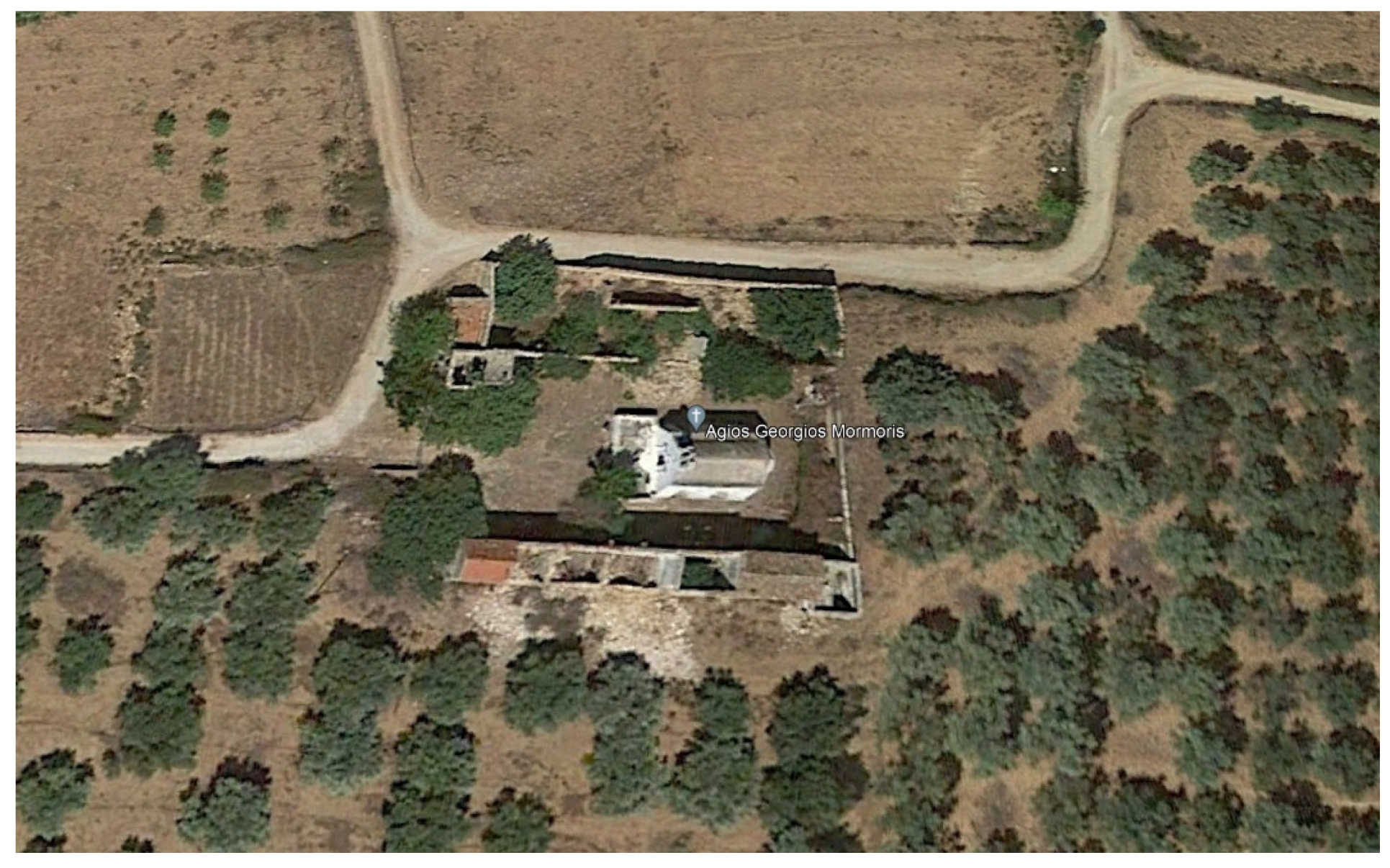
In Greece’s Crete area, the chapel of Saint George Mormoris was the focus of the present case study. The Holy Monastery of Saint George Mormoris is situated in a small urban area close to the city of Chania in western Crete (Figure 1). The entire structure was constructed in the 17th century. It was reportedly built before 1637 under the Venetian Dominance in Crete. The now-abandoned monastery is part of the Gouverneto Monastery and is a protected landmark.

The whole complex currently comprises the historic Church of Saint George Mormoris in the middle, a historic olive mill, monastic cells, and warehouses. The church is surrounded by a rectangular enclosure with warehouses, an olive mill, and monks’ homes.

The small chapel with its stone masonry walls was constructed during the 18th and 19th centuries. Its barrel-roof building is indicative of Venetian architecture. The masonry walls of the chapel are composed of stones and are strengthened by six buttresses at the corners and in the centre of the north and south walls. The roofing is composed of barrel-shaped stones. The ground surrounding the church consists primarily of small raw stones, sand, and loose natural soils. At the entrance of the church, a concrete slab was created to improve the ground-bearing capacity (Figure 2).

Plaster is applied to the masonry walls. Even if the structural system is covered by plaster, it may be distinguished by the exfoliation of the mortar, which is mostly produced by mould and hives/cells. There are little cracks on every wall. On the northeastern side of the building, a larger crack can be seen, revealing the potential location of ground subsidence.

This property was chosen since it is not located near noisy roadways, making it simpler to identify the building’s modal features without having to eliminate external noise. It also offers a plan view that is simply specified and can be quickly modelled and validated using the finite element method (FEM).

4. OMA’s Measurement Survey Setup

The entire experiment was carried out in September 2022. Throughout the whole operation, the weather was primarily sunny with clouds and light winds.

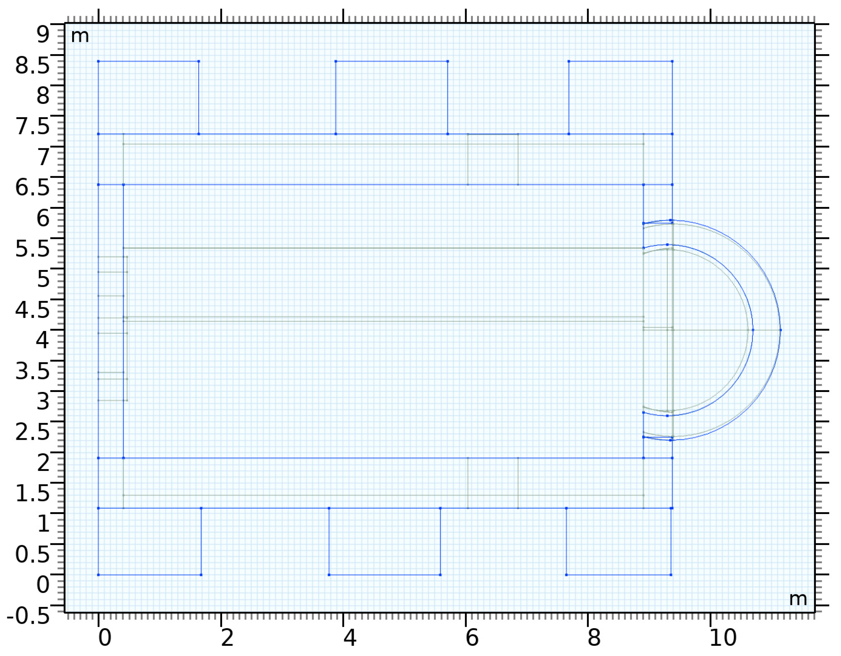
The analyzed structure was surveyed and modelled before taking measurements using a Polytec scanning laser Doppler vibrometer [28]. The horizontal layout of the chapel’s main construction is roughly 6.2 m by 9.3 m, and its south and north masonry walls are supported by six buttresses, three on each side, working against the lateral stresses coming from the inadequately braced roof structure (Figure 3, Figure 4 and Figure 5).

The scanning laser Doppler vibrometer (SLDV) employed in this study is a Polytec PSV-H-500 system equipped with its main controller, 1D single-point measurement laser head, with resolution 0.25 nm, constant in the entire frequency range of 0 Hz to 100 kHz, laser beam wavelength 633 nm (red light)-473 THz EM wave, and vibration amplitudes range of 1 mm/s–10 m/s. In addition, the Polytec PSV-H-500 features a multichannel analogue or digital input signal acquisition unit and a geometry scan unit (Figure 6).

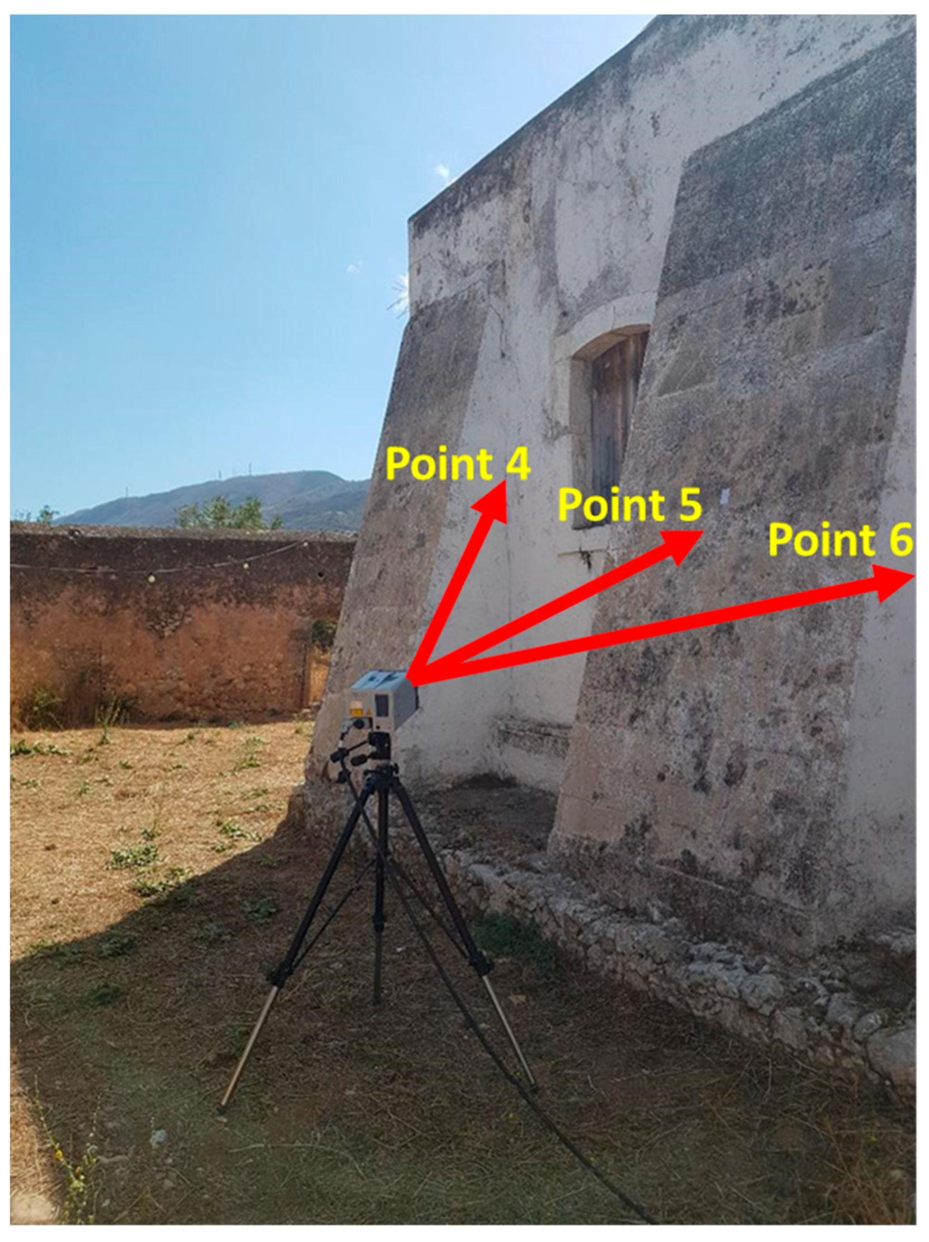
Based on the weather conditions, the position of the scanning laser head was selected, and it was placed at a distance from each wall. At the measurement places, reflective tape was applied to improve the signal to the laser head. The laser vibrometer PSV-500-H is equipped with two computer-controlled mirrors that allow the operator to select a measurement point on a test sample, measure the response, and then proceed to additional measurement places without having to move the instrument. This process was conducted a number of times until all scanning sites were measured and a comprehensive map of the surface motion was compiled. Thus, SLDV is able to directly measure the moving surface of a large area, even if it is at a problematic angle and orientation.

A conventional ICP contact single-axis accelerometer sensor of type PCB model type 352A78 [29] with 100 mV/g sensitivity, +/−50 g pk measurement range, and 0 to 15 kHz frequency range capabilities equipped with an ICP battery-operated signal conditioning unit of type 480C02 was installed on the west wall as a reference sensor, remaining, in the same location for all measurement setups, between the main entrance of the chapel and the first buttress on the PCB accelerometer sensor continuously detects the acceleration of a response that remains stationary during the measurement (Figure 7 and 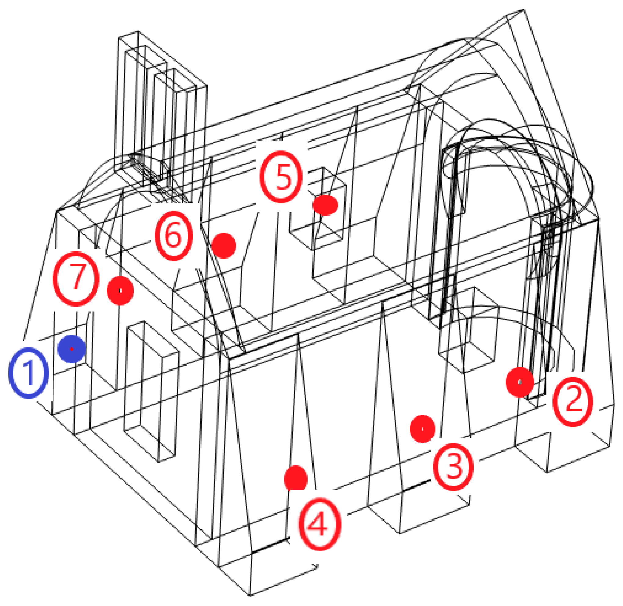Figure 8). This accelerometer sensor’s analogue signal is utilised to time-reference the point-by-point SLDV signals. To investigate the overall investigated structure, six setups were defined in this study. A setup consists of an array of the two instruments, reference PCB single-axis accelerometer sensor and SLDV, where the accelerometer sensor is in the same position for all setups, and the SLDV acquires velocity signals at two stations, one on the southern side of the structure and one on the northern side, with three laser beam target points for each station (Figure 8 and Figure 9). Throughout each setup, the examined structure is captured for a minimum of 10 min. Figure 7, Figure 8 and Figure 9 depict the locations of the reference accelerometer sensor and the six different laser beam target positions.

The automated remote measurement survey with the PSV-H-500 system is conducted as follows: (1) Retroreflective items, such as tapes, are mounted to the measurement points. (2) The direction of the laser head is adjusted such that the SLDV’s reflection level achieves its maximum. (3) Setting the measurement duration and sample frequency. (4) Each measurement point is surveyed by the PSV-H-500, and the geometry scan unit’s positional data are then recorded within. (5) When the PSV-H-500 laser target spot automatically hits a measurement point using the stored information, data acquisition proceeds concurrently using both the SLDV velocity input signal and the reference PCB acceleration input signal. (6) As soon as the SLDV vibration measurement is completed, the PSV-H-500 moves automatically to the next measurement site, while the reference PCB accelerometer sensor stays in place. After completing measurements at all scan sites, the device can automatically repeat measurements. In the present investigation, vibration measurements are taken at two separate locations (stations) of the scanning head: one on the southern side of the chapel and the other on its northern side. For each laser head station, the SLDV scans three spots automatically.

5. Operational Modal Analysis

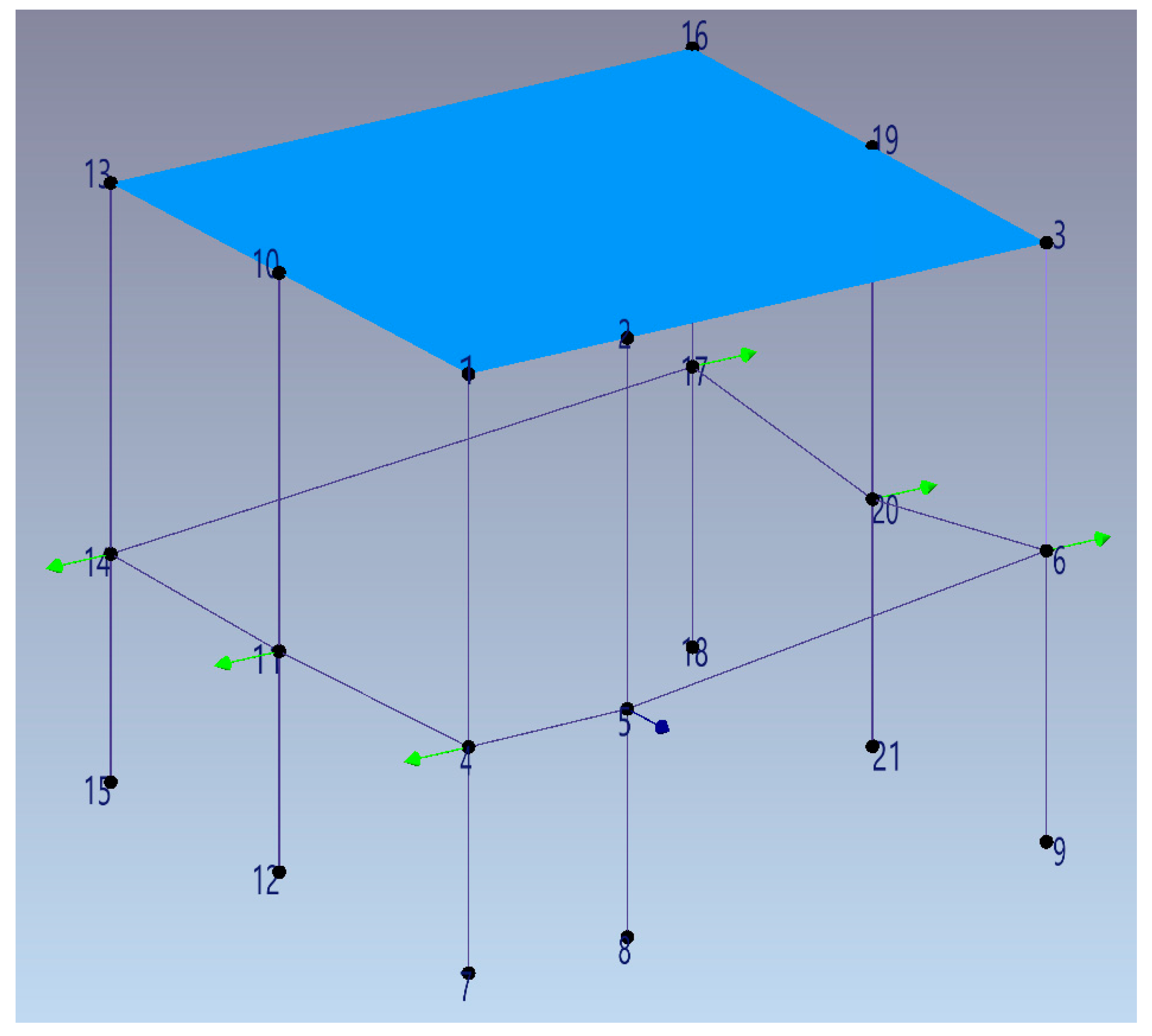
The ambient vibrations generated by environmental loads (mostly low wind excitation as the case study region is away from vehicular traffic in operating conditions) were measured. Six time series of 600 s were recorded to confirm the quality of the data. Using the frequency domain decomposition (FDD) approach, also known as the Peak–Peak method, and the ARTEMIS Modal Standard software [30], the modal parameters of the structural system were determined. The simplified 3D wire frame of Figure 10 depicts the geometry of the examined structure, as determined by the measurement points at the six setups, and their corresponding locations on the structure.

The FDD method automatically calculates the modal parameters from the signal processing data. It makes use of the fact that the mode shapes may be approximated from the computed spectral density when random noise or stochastic input is given to a system with well-separated modes and light damping. It is decomposed using singular value decomposition (SVD) at each spectral line, where the PSD matrix is divided into auto spectral density functions consisting of single-degree-of-freedom systems. By detecting the peaks in the SVD plots, the modes are identified. The precision of the approximated natural frequency is dependent upon the FFT resolution.

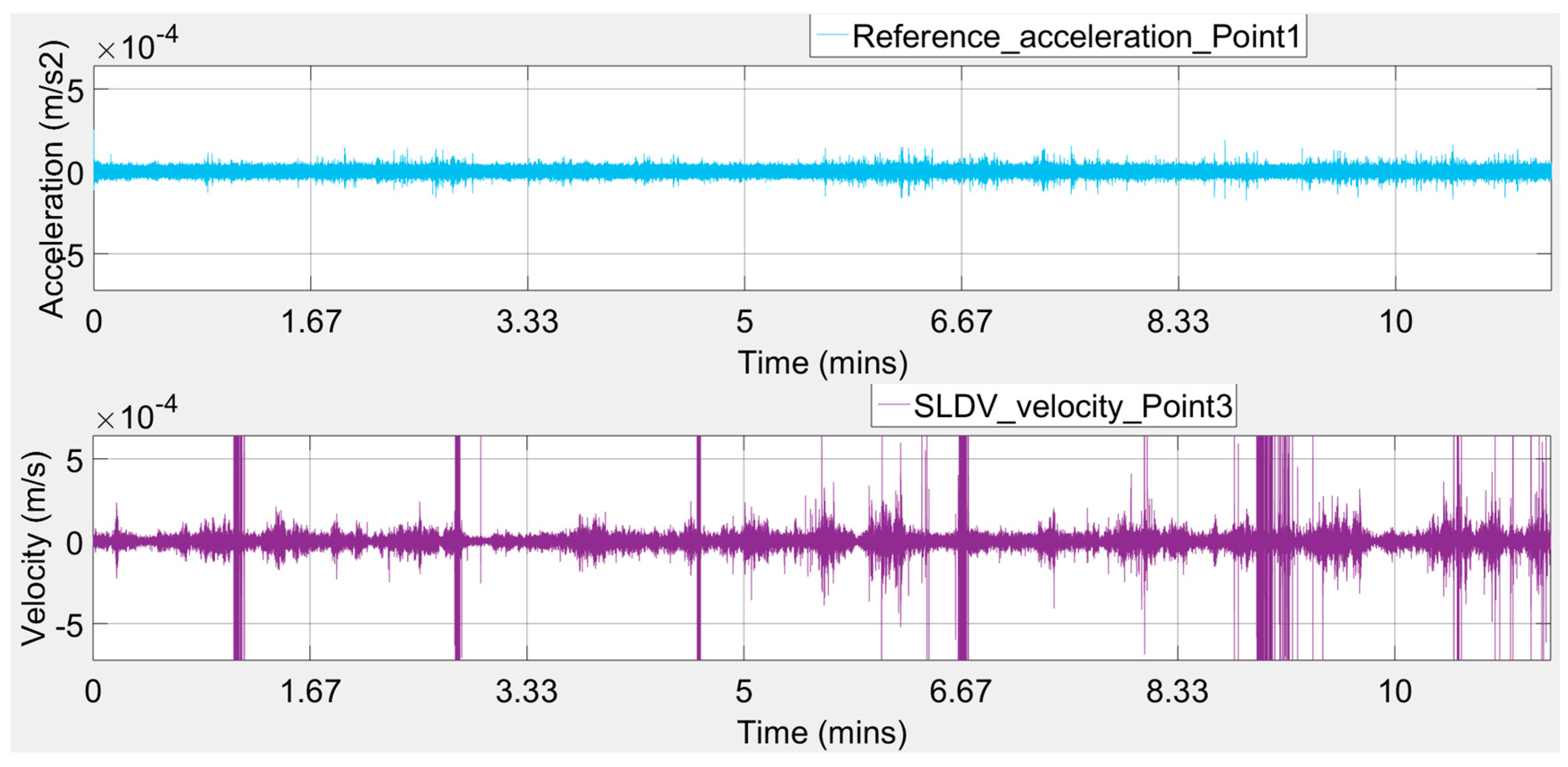
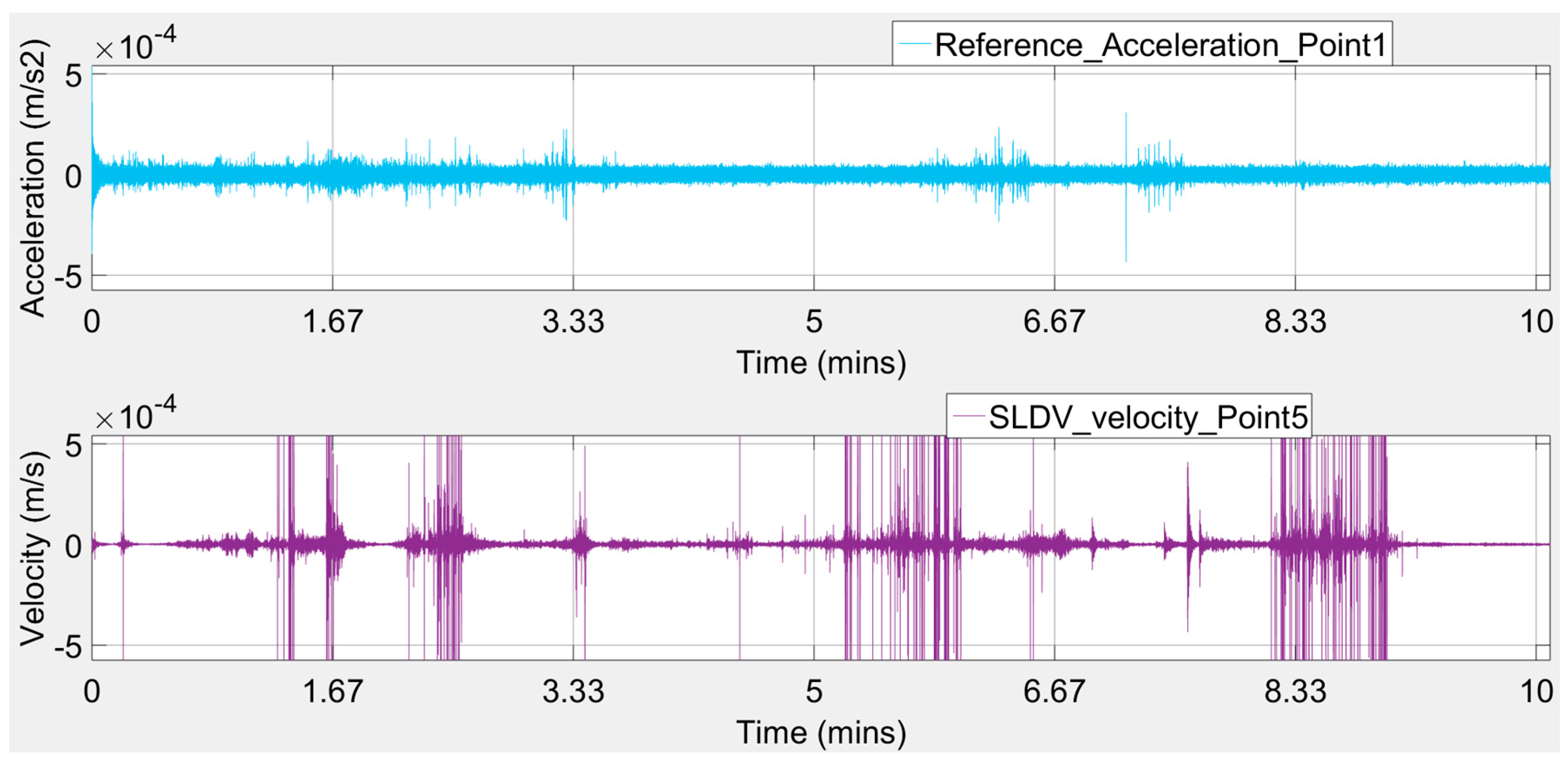
Figure 11, Figure 12, Figure 13, Figure 14, Figure 15 and Figure 16 depict the measured acceleration records at the reference location (see Figure 9—Point 1) and the corresponding measured velocity records for each of the SLDVs target spot points (see Figure 9—Points 2 to 7). Signal intervals affected by irregular spikes or unexpected vibration levels were excluded from the analysis. Note that the recorded movement has a very low amplitude (about 4.0e⁻⁴–5.0e⁻⁴ m/s²), which is a feature common to ambient vibration in stiff structures.

Observing the plots of Figure 11, Figure 12, Figure 13, Figure 14, Figure 15 and Figure 16, it seems that there were intense peaks in the frequency domain, probably caused by the wind gusts putting some blast pressure waves on the investigated walls of the case study building.

Additionally, it is well known that when we have a testing procedure with a single-input-single-output system case, for each frequency, the coherence between the system’s input signal and the system’s output signal provides a measure of the extent that each output signal can be linearly explained from the associated input signal. A coherence of 1 indicates that the output signal can be completely linearly explained from the input signal; a coherence drop below 1 indicates that the output signal can only partly be linearly explained from the input signal and that there may exist a nonlinear relation between the input and output signal and/or there is contaminating noise in the input signal and/or output signal, while a coherence of 0 indicates that there exists a nonlinear relation between the input and output signal. From the extracted accelerometer and SLDV signals, as plotted in Figure 11, Figure 12, Figure 13, Figure 14, Figure 15 and Figure 16, after some filtering process performed automatically by the ARTEMIS Modal software, it may be observed that when the input excitation acceleration in the direction of the -Y-axis of the reference accelerometer at Point 1 is excited, the +X-direction of the SLDV output velocity recordings at Points 3 and 4 and the -X-direction of the LDV output velocity recordings at Points 5, 6, and 7 coherences are close to one (in the range of 0.75 to 0.95). However, the one coherence in the +X-direction of LDV output velocity recordings at Point 2 is not sufficient. One possible explanation may be that the structure stiffness may be changed when the X-direction is excited with an ambient vibration, which results in the nonlinearity between the -Y-direction input and +X-direction output. This issue, as stated above, is automatically resolved by the software ARTEMIS Modal by modal filtering from the frequency domain with the usage of inverse fast Fourier transform.

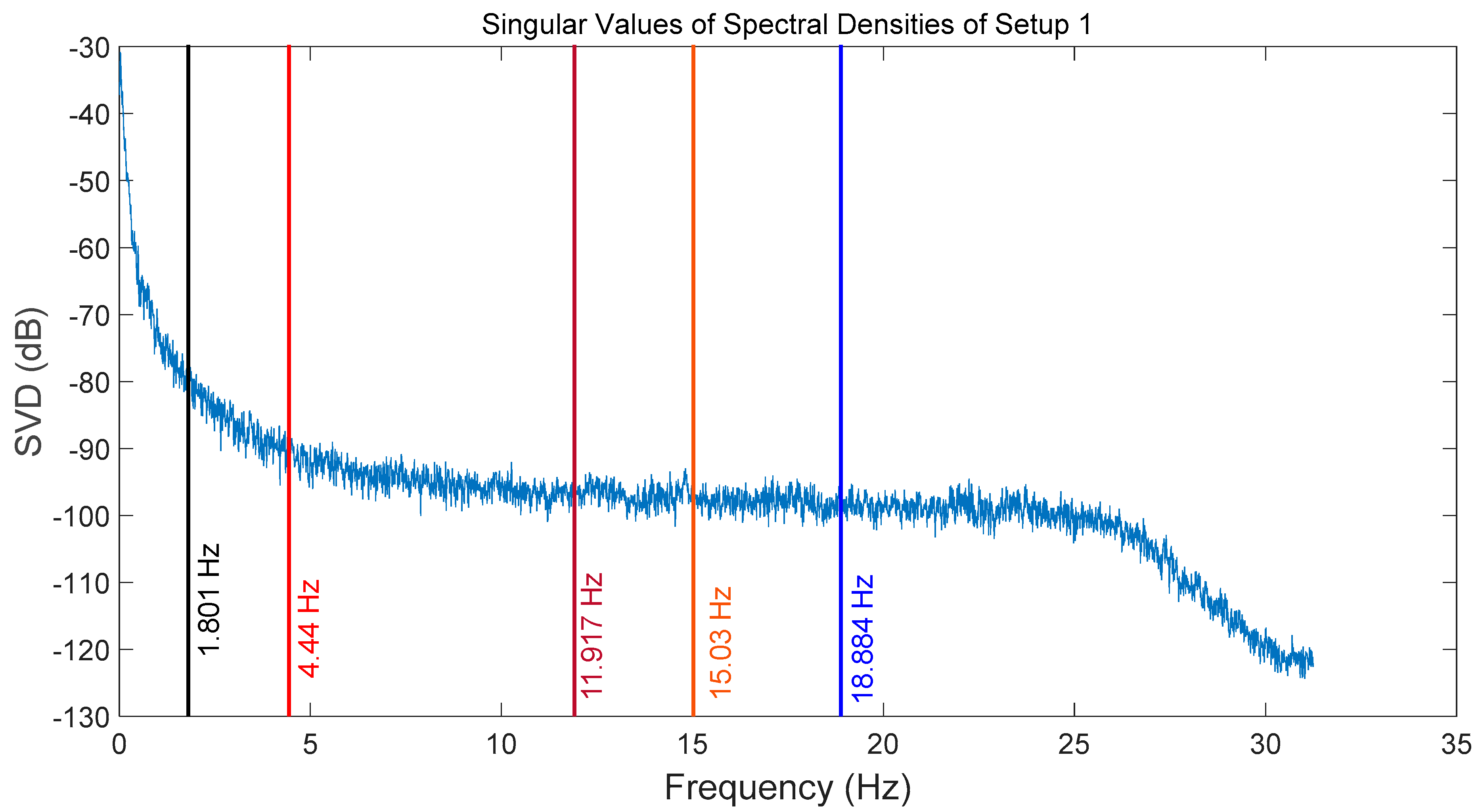
Figure 17 illustrates the singular value decomposition (SVD) plot of the spectral densities for the first setup: SLDV beam targeting at Point 2, where the distinction between each mode is unclear, while Figure 18 plots the average SDV of the spectral densities for all setups. Contrary to the unclear distinction of modes in Figure 17, the modes in Figure 18 are easily identified.

6. FE Model Updating and Calibration

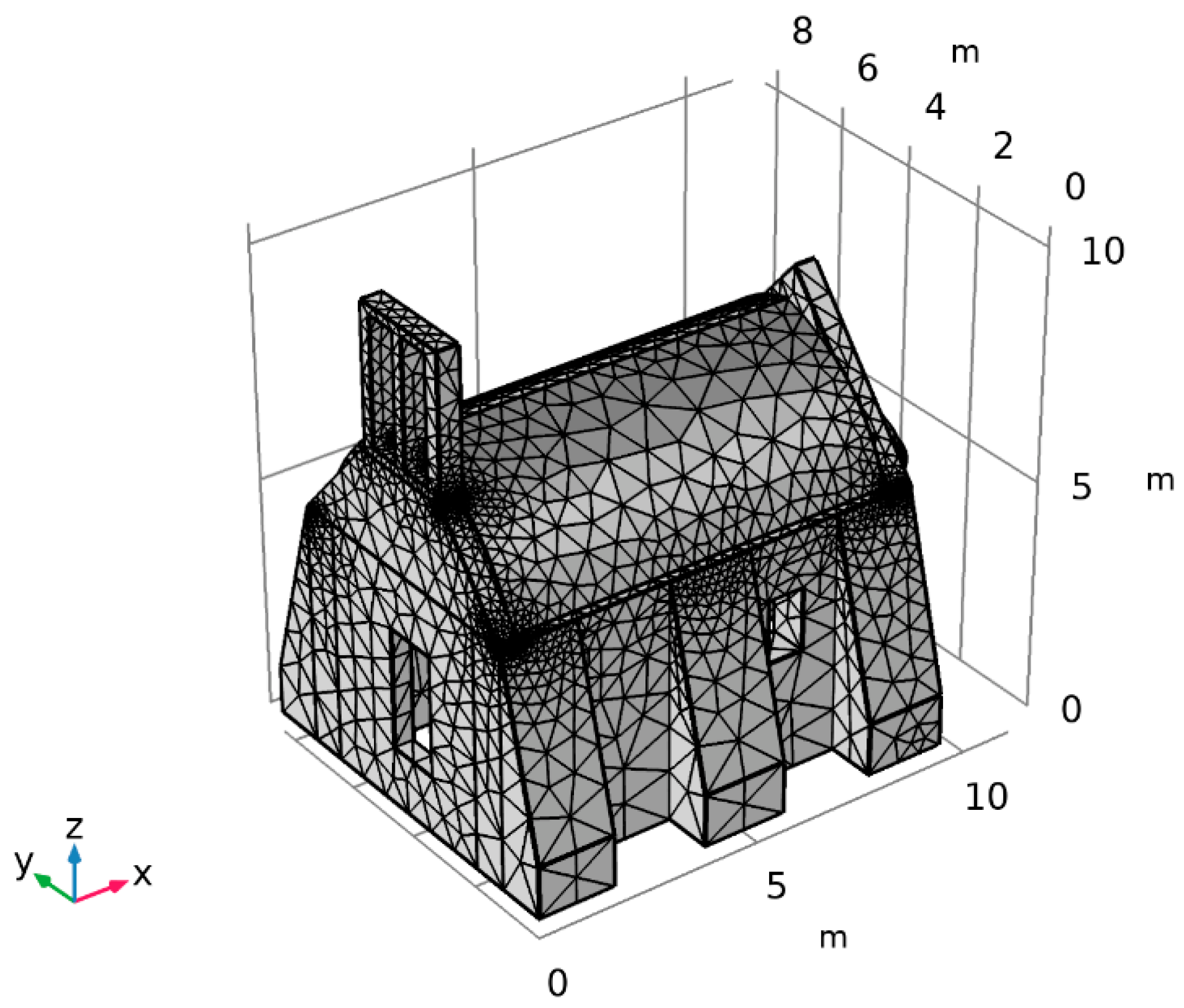
The COMSOL Multiphysics package [31] was used to create a 3D finite element (FE) model based on data acquired from both topographic surveys and historical documentation. As a result, solid 3D finite elements were used to discretise the geometric model. FEs were subsequently classified into sub-parts based on structural and typological similarity (i.e., side walls, barrel-type roof, buttresses, arches, domes, etc.). The FE model seen in Figure 19 is mostly composed of quadratic tetrahedral components with 10 nodes and 3 translational degrees of freedom per node. The quadratic feature of the components assists significantly in convergence when constructing a model of natural frequencies. The overall model consists of 11,642 nodes, 40,503 degrees of freedom, and 58,211 elements. Figure 20 displays the created 3D FE model and its sub-parts in different colours. In total, eleven separate sub-parts were individuated at different regions of the structure.

The FE model of the structure is updated with regard to the experimental data such that its modal characteristics correspond as close as possible with the experimental ones. To this purpose, a collection of unknown structural parameters is assessed from the minimisation of an objective function defined as the difference between observed data and numerical forecasts. The assessment of numerical modal parameters is time-consuming due to the complexity of the numerical model, and the success of the optimisation issue is greatly dependent on the effectiveness of the optimisation procedure. Consequently, a sensitivity analysis (SA) is conducted first in order to select the most appropriate mechanical characteristics of the eleven sub-parts and limit the number of objective function evaluations. In the current SA, the natural frequencies and related mode shapes are explored in response to modifications in the unknown structural parameter of eleven sub-parts in order to determine which parameter significantly affects the dynamic response of the inspected structure.

There are several approaches to sensitivity analysis (SA) that explicitly describe different “understandings” of the sensitivity of one or more model responses to various inputs, such as model parameters. The relevance of SA and the associated challenges in the context of FE model updating cannot be underestimated. Such FE models are gradually becoming significantly more complicated and computationally costly, enhancing dimensionality (both process and parameter) (both process and parameter). Despite the fact that SA has become a crucial tool in the creation and use of such models, its usability might be limited by computational cost. 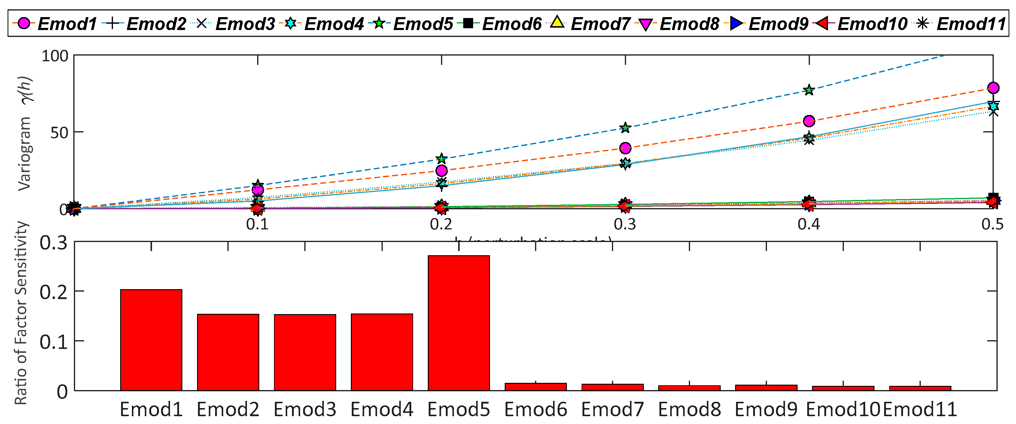Thus, for the sake of the present research, we determined that our approach to sensitivity analysis should be based on the MATLAB toolbox VARS TOOL based on the Variogram Analysis of Response Surfaces, which is a recently released GA technique established in [32,33,34,35]. Variograms are effective tools for describing the spatial (or spatiotemporal) structure and variability of a dependent variable within a space generated by a collection of factors. This is related to a characterisation of the “response surface” of a model, which depicts how a goal response (a state or output variable or a performance metric) changes with one or more elements of interest in the context of computer simulation models. As such a performance metric in this study, we offer the function H(x) of Equation (1), which can be thought of as a measure of the difference between numerical and experimental natural frequencies and mode shapes for the five modes shown in Figure 18:

$$H\left(x\right)={{\displaystyle \sum }}_{j=1}^N\left[a{\left(\frac{f_{exp,j}-f_{num,j}}{f_{exp,j}}\right)}^2+\left(1-a\right){\left(\frac{1-MAC\left({\phi }_{exp,j},{\phi }_{num,j}\right)}{MAC\left({\phi }_{exp,j},{\phi }_{num,j}\right)}\right)}^2\right]$$

(1)

where x is the vector representing the unknown parameter for each of the 11 structural sub-parts, and N is the number of modes examined in the calibration operation (N = 5 in the present analysis). Lastly, MAC represents the correlation between two modal vectors and is the Modal Assurance Criterion. Eleven variables that comprise the FE model were modified during the SA. Particularly, the eleven elastic moduli of the eleven sub-parts into which the FE model was separated were utilised and given the designations Emod1, Emod2 up to Emod11. The lower and higher limits of these variables were chosen to determine substantial differences in the natural frequencies and mode shapes of the FE and to provide relevant information for addressing the updating problem. In particular, it was expected that the elastic moduli varied between 1 × 10⁵ Pa and 1 × 10 Pa. It is thought that such a lower bound for the sensitivity parameters is due to the severe damage state, the great age of the structure of interest, and the absence of knowledge regarding the mechanical characteristics.

Adopting the VARS TOOLS in the current SA and given the above-mentioned function H(x) as the FE model response due to the set of 11 elastic moduli parameters, i.e., y = f(x) where x = {Emod1, Emod2, …, Emod11}, the global sensitivity of y with respect to xj is a scale-dependent property that can be characterised using the variogram and covariogram functions γ(h) = 1/2.V(y(x + h) − y(x)) and C(h) = 1/2.COV(y(x + h), y(x)) where h = x_A − x_B is the vector representing the distance h = {h₁, h₂, …, h₁₁}, between any two points A and B in the factor space. Directional variograms (hi) and covariogram C(hi) can give a wealth of data regarding sensitivity throughout the whole range of scales. This information may be defined by a collection of metrics known as IVARS (integrated variogram across a range of scales), which are derived by integrating the variogram to a scale (hi) of interest. 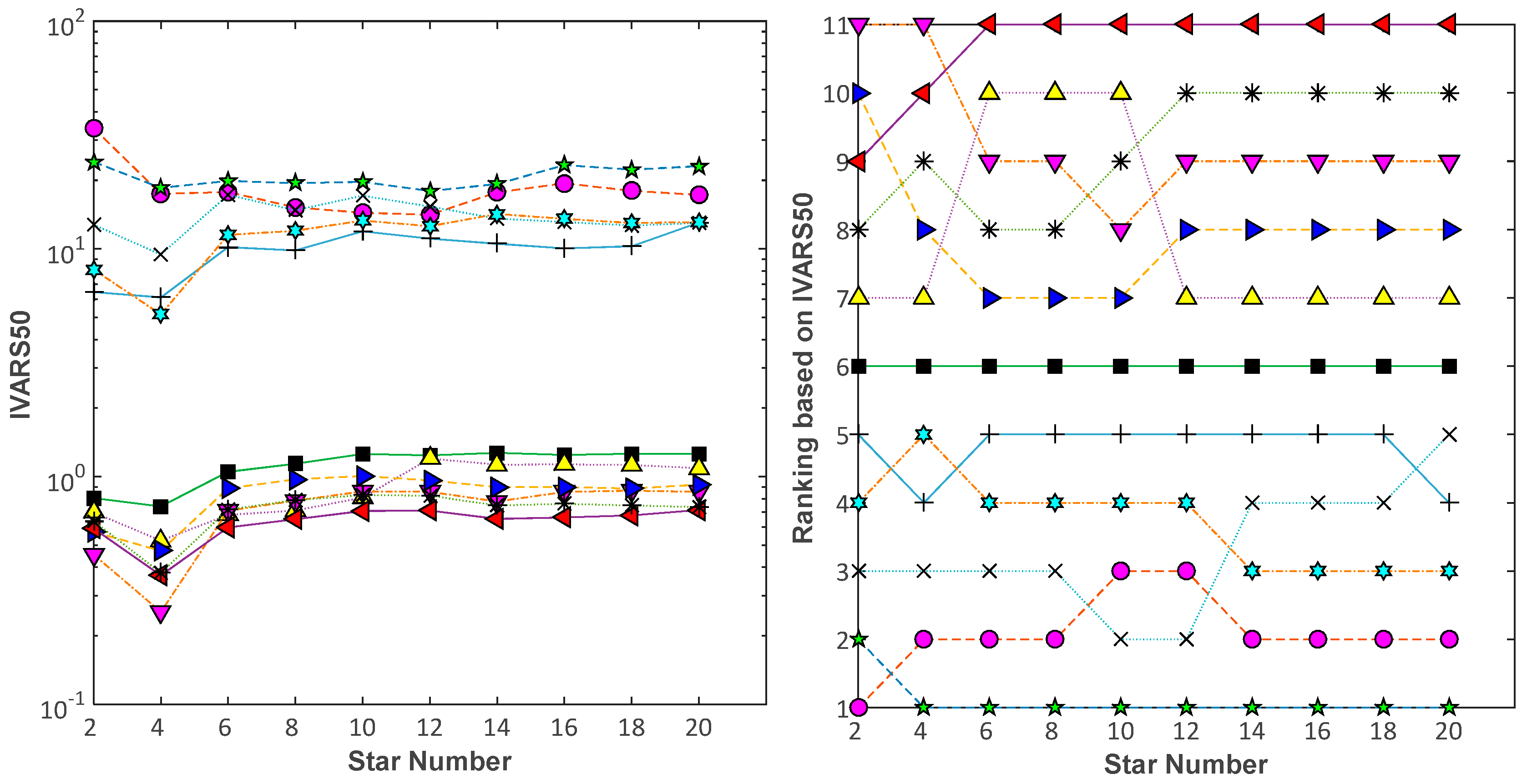According to Razavi and Gupta ([32]), it is advised to utilise Hi values that correspond to 10%, 30%, and 50% of the factor range, yielding IVARS10, IVARS 30, and IVARS50, respectively. Here, IVARS50 was utilised as the sensitivity metric for the eleven elastic moduli. We define, based on the fundamental features of variograms, that a greater value of IVARS50 for any particular hi implies a greater rate of sensitivity of the underlying variable.

According to the execution of VARS TOOL and the findings provided in Figure 21 and Figure 22, the first five elastic moduli (Emod1, Emod2, Emod3, Emod4, and Emod5) of the eleven sub-parts influence the dynamic response of the investigated structure much more than the remaining six elastic moduli. Then, based on the previously mentioned sensitivity analysis, an FE model updating approach is carried out by selecting as parameters of the updating operation any or some of the first five of the eleven elastic moduli in order to identify the most important parameters to be updated.

The process of updating the FE model was conducted by minimising the difference between frequency and MAC values, as described by the metric H(x) in Equation (1), while varying the elastic moduli of the five sub-parts within their physical ranges. This problem may now be seen as a multivariable optimisation problem with a single objective, namely objective function (see Equation (1)). MATLAB Optimisation Toolbox’s Genetic algorithm [36] was utilised for the optimisation procedure. In the present GA analysis, the optimal value of the specified elastic moduli is determined using, as the objective function, the function H(x) of Equation (1). A binary encoding technique is applied in the present GA, where the length of the code chain is dependent on the number of chosen elastic moduli. As input data, the initial values of elastic moduli for the sub-parts of the simulated FE model are entered. The GA analysis is then initiated with a random population. The code chains of the individual values of the chosen elastic moduli in the population are solved, and appropriate values are assigned to the elastic modulus of structural components. The following phase involves calculating the objective function value H(x) for each individual value of elastic moduli in the population (generation) for each ith mode.

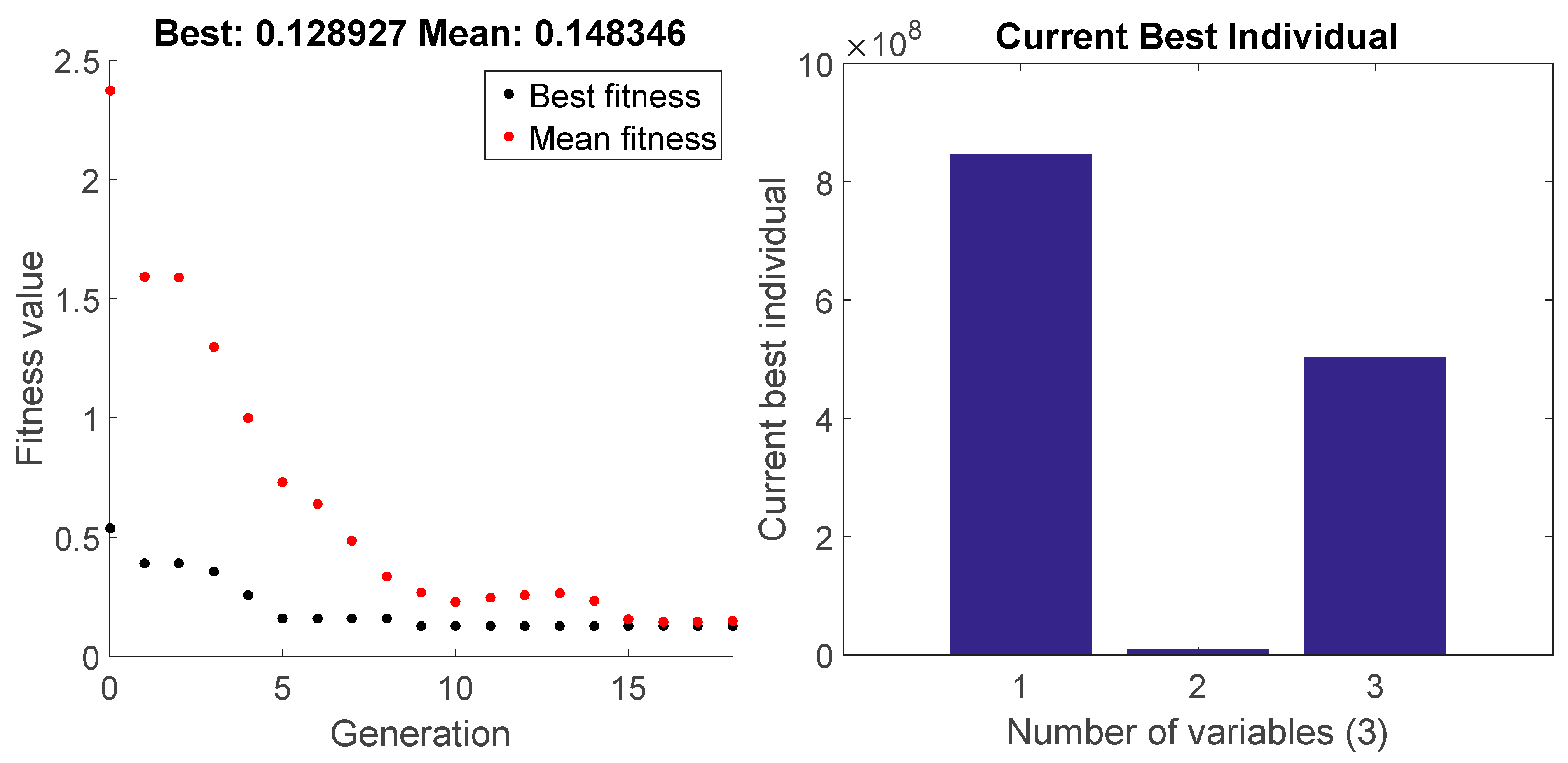
All GA phases are repeated until the total value of the objective function H(x) equals zero. When the total objective function value is equal to zero, the GA minimises the difference between the updated simulated FE model response and experimental data; hence, the two models are identical. The following phase involves applying GA operators (reproduction, double-point crossover, and mutation) to the generation. In the reproduction operator, the individuals with the best values (near to zero) of the objective function are allowed to remain in the population, while the people with the worst value are removed from the population and replaced with copies of the best individuals. Consequently, the number of individuals in the population remains unchanged.

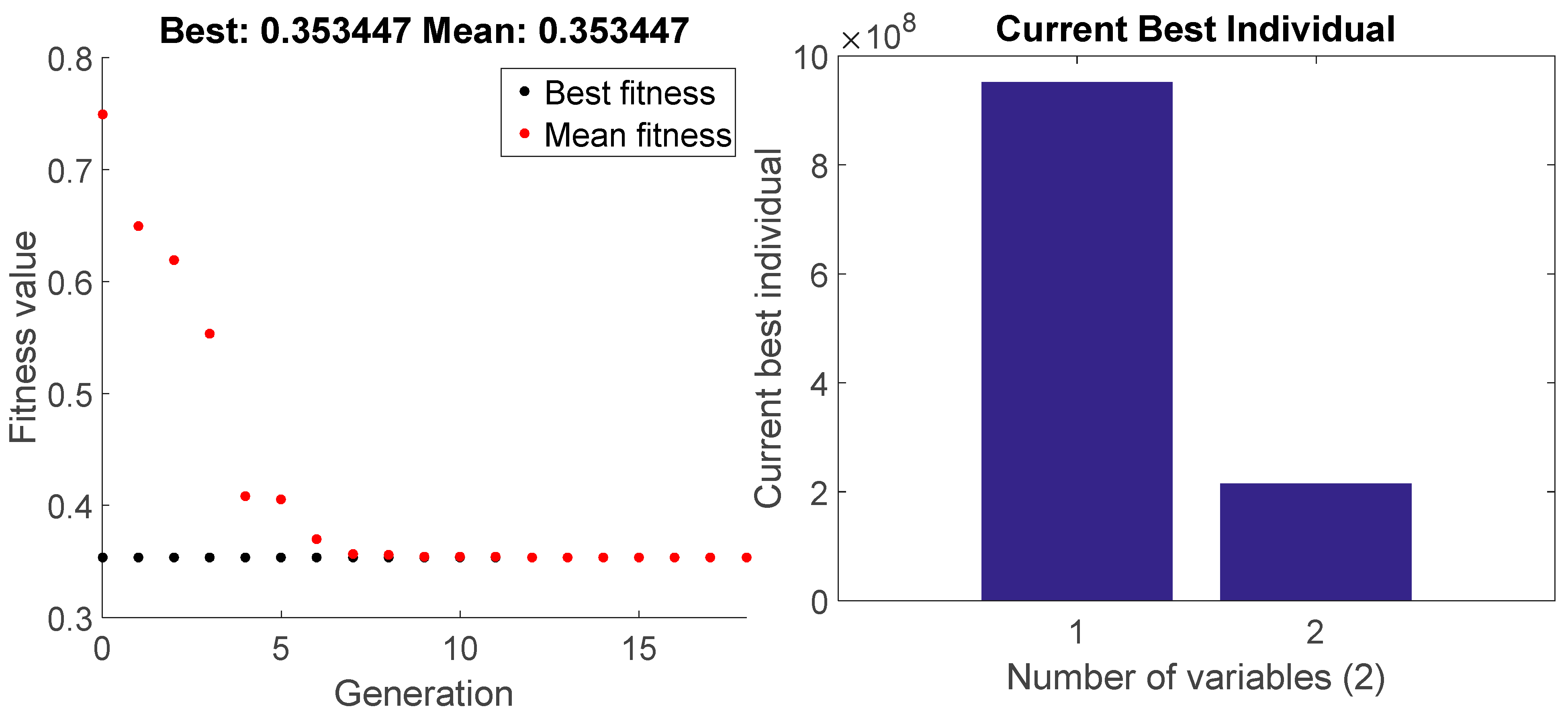
Following the application of the crossover operator to the population, the mutation operator is applied to all individuals with a predetermined probability. Individual codes are transformed from 0 to 1 or 1 to 0 at random. Finally, the subsequent population is superior to the prior one. All aforementioned GA stages are repeated until the value of the objective function H(x) equals zero (Figure 23). In this work, a MATLAB code for FE updating is developed to link the FE model generated in the COMSOL package with the execution of the GA algorithm in the MATLAB Optimisation Toolbox.

A first rough manual tuning step of the elastic moduli was carried out with respect to the five natural frequencies presented in Figure 24 and Figure 25. Then, the process of FE model updating was carried out for the minimisation of the objective function value of H(x) with an initial value of 1 × 10⁶ Pa and a uniform distribution of elastic moduli over the whole structure. After 500 iterations, the optimum value for the common elastic moduli was 65.2 MPa, and the best value for the objective function was 0.418549, as seen in Figure 24 and Figure 25.

The second tuning step (on the elastic moduli) was performed by altering just the values of elastic moduli Emod1 and Emod5 of the 1 and 5 sub-parts, respectively, of the inspected historical structure. As illustrated in Figure 26 and Figure 27, the selection of only those two elastic moduli was based on their substantial sensitivity influence on the fluctuation of H(x). Assuming that the configuration of the other sub-parts remained unaltered, the elastic moduli were set to the value obtained during the initial tuning step. The GA optimisation method for the second tuning step resulted in new calibrated values of 952.38 MPa and 215.38 MPa for Emod1 and Emod5, respectively, while the best value of objective function H(x) equalled 0.353447, as depicted in Figure 26. In comparison to the first tuning step, the optimal objective function value H(x) decreased by around 15%. Figure 27 and 36 plot the GA findings for the distribution of the elastic moduli for the whole structure.

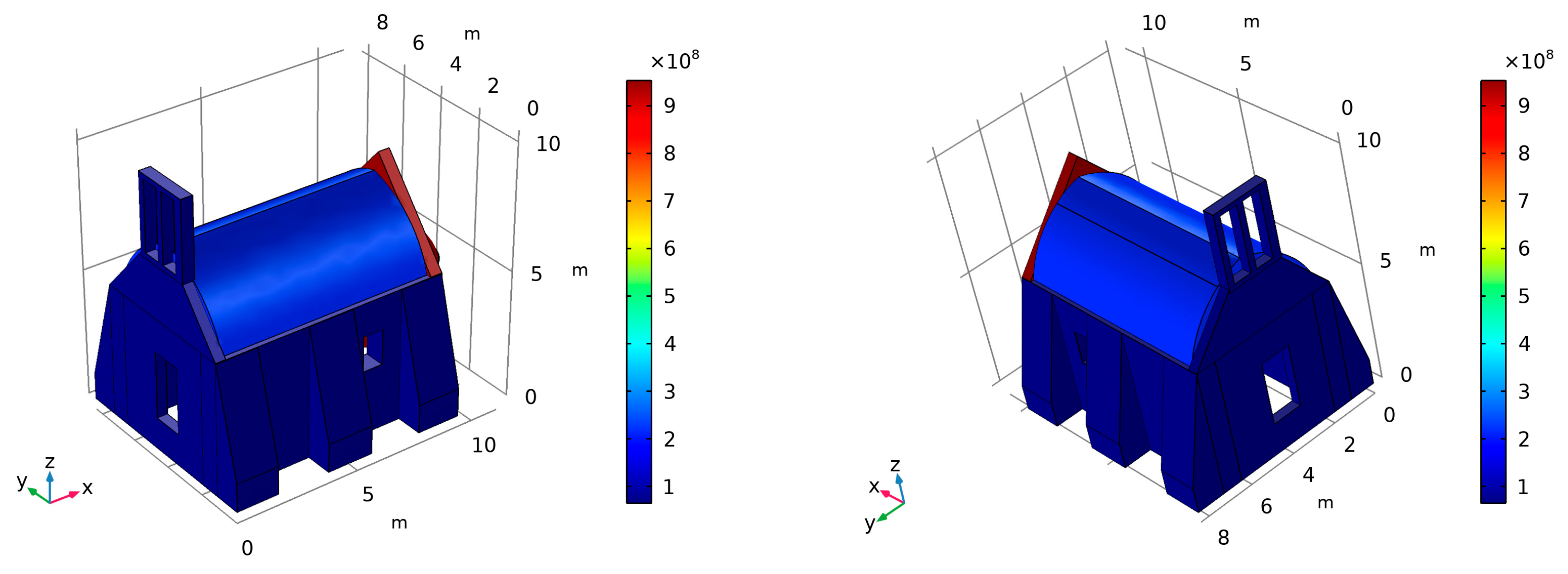
In an effort to further enhance the findings of the FE model update, a third tuning step was implemented by altering the values of just the three elastic moduli Emod1, Emod3, and Emod5 of the 1, 3, and 5, respectively, sub-parts of the inspected masonry structure. The three elastic moduli were introduced in the GA Optimisation process with starting values of 1 × 10⁵. The GA optimisation method for the third tuning step yielded a higher value for Emod3 compared to the first tuning step; however, the newly calibrated values for Emod1 and Emod5 were roughly equivalent to those of the second tuning process. Figure 28 and Figure 29 exhibit the outcomes of the third tuning step. The optimal value of the objective function was 0.128927. The optimal objective function was reduced by 69% compared to the initial tuning step.

In particular,

Table 1. Experimental frequencies vs. numerical frequencies after updating steps.

Modes	Experimental Frequency (Hz)	1st Tunning Numerical Frequency (Hz)	2nd Tunning Numerical Frequency (Hz)	3rd Tunning Numerical Frequency (Hz)
1	1.801	1.756	2.164	1.878
2	4.44	4.609	4.421	4.146
3	11.917	11.972	11.954	11.868
4	15.03	14.930	14.959	15.051
5	18.784	18.822	18.617	18.751

reports the values of the updated parameters compared with the initial ones;

Table 2. Elastic moduli after updating steps.

Tuning Process	Emod1	Emod2	Emod3	Emod4	Emod5	Objective Function Value H(x)
1	65.2 MPa	65.2 MPa	65.2 MPa	65.2 MPa	65.2 MPa	0.418549
2	952.4 MPa	65.2 MPa	65.2 MPa	65.2 MPa	952.4 MPa	0.353447
3	846.8 MPa	65.2 MPa	8.4 MPa	65.2 MPa	503.3 MPa	0.128926

shows the results of the updating procedure reported in terms of the final modal frequencies of the structure, together with their relative differences. The variance between the experimental modal frequencies and the numerical natural frequencies was decreased by approximately 70% following the third tuning update procedure.

7. Discussion and Suggestions

The structure’s natural frequencies extend to a wide band in the 1.8 to 18.8 Hz range, which is a common frequency band for this kind of structure. The final frequency errors for all tuning stages show that the presented results are adequate because the major error was not more than 6.5%, and the final MAC values were also adequate because the related error maintained approximately the same value between stages—not more than 5%.

We decided to use the elastic modulus of stone masonry as the most important calibration parameter for the model updating since prior evaluations show that the value H(x) of Equation (1), which is an indication of differences between experimental and analytical models, has stronger changes in the variation of this calibration parameter.

Several different weighting factors α of Equation (1) were tested to evaluate their effect on model selection. For the range of interest for the values of elastic modulus, located between the values of 1 × 10⁶ and 1 × 10 MPa, the frequency participation was not like the weighting factors entered. It is noted that for the case where the factor α = 0.5 (the frequencies and MAC index weigh the same), the frequency term had a 10% participation in the H(x) value and, correspondingly, the modal shape term would present 90% participation within the area of interest. For the case in which the weighting factor in the frequency term was 0.90, its participation reached approximately 60% of the H(x) value. We, therefore, finally chose to work with this last case, e.g., α = 0.90, to evaluate the results. Similar results have been presented in the work of Torres et al. [37].

Based on the experience gained during the research, some suggestions can be made to help future research studies or engineering projects. The referential accelerometer sensor must be located in places of the structure where the expected movement is as high as possible for most modes. The SLDV beam ray should be successively targeted to points that should be distributed on the inspected structure based on the modes the user wants to capture. Other factors to consider in the experimental campaign using SLDV equipment are: precise 2D and 3D alignment for the velocity direction determination, improved signal quality for the measuring surface of the masonry building if it is non-cooperative with poor back-scattering properties, high synchronisation of the accelerometer sensor with SLDV sensor, and finally good sensitivity to base vibrations since it is a strong limitation factor for SLDV applications on harsh industrial cases.

In our integrated method, we employ an accelerometer as the reference acceleration signal sensor and an SLDV as a multiple velocity output sensor that can scan the velocities at a large number of monitoring sites utilising each of them as a different output signal sensor. The use of SLDV as a multiple output sensor significantly extends measurement capabilities compared to conventional vibration sensors (such as accelerometers), as it enables “remote”, non-intrusive, high spatial resolution measurements with reduced testing time and improved performances at distances greater than 30 m with sufficient accuracy (1–2.5% RMS of reading) (high-frequency bandwidth, wide velocity range, high resolution in displacement and velocity). In addition, the scanning capability of SLDV allows the measurement point to be moved swiftly and accurately on the structure being tested, enabling the examination of a vast area with great spatial resolution and little testing time. Due to the fact that an accelerometer can only measure one single point at a time, the data-gathering phase becomes a significant component of the whole project. Therefore, if we exclusively employ accelerometers in the proposed research, as the reviewer states, we can only provide as much data as there are available accelerometers.

Furthermore, utilising a laser vibrometer for a historic building vibration measuring programme is significantly faster than using accelerometers since the time saved during the setup of each measurement point significantly outweighs the time wasted during measurements. Since contactless laser vibrometer systems require less equipment and less time, they are a more economical alternative to conventional accelerometer-based techniques. In addition, laser vibrometers are often fairly portable.

Certainly, an SLDV is a relatively expensive piece of equipment, but given that SLDV set-up time is only a few minutes per location and that technicians are paid EUR 100 to 150 per hour on site, lowering set-up time would create considerable cost savings for customers. In addition, for a comprehensive evaluation of this historic structure, utilising exclusively accelerometers, simultaneous or sequential measurements should be used. The simultaneous technique often employs many accelerometers simultaneously. Assuming there are sufficient accelerometers, signal cables, and input channels on the frequency analyser (these devices typically handle 8, 16, or 32 channels), many measurements can be performed concurrently. Nonetheless, this necessitates the installation of several accelerometers (more than 50 in our case study) and signal lines while preventing cable confusion.

As illustrated in Figure 19 and Figure 20, the FE model is based on some assumptions. First, the behaviour of the structure is assumed continuous, with no discontinuities at wall intersections. Second, the structure’s highly flexible components (small bell tower) have been simplified because the rigid component of the structure is the central focus. Finally, the elastic moduli of the structure may be defined by representative values with a high degree of variation in eleven distinct structural zones. Taking into account the aforementioned assumptions, we pre-examined different meshing schemes to minimise the influence of the FE meshing and smoothing some serious geometric singularities on the 3D model that affect the accuracy of the numerical results. Finally, we decided to settle on a scheme of the FE model comprised primarily of quadratic tetrahedral elements of 10 nodes (CTE10) with three degrees of freedom (translational) per node. The quadratic feature of the components assists significantly in the convergence when constructing a model of natural frequencies. There are 11,642 nodes in the whole model, of which 3022 are totally limited at the base. Therefore, for the present case study, a total of 40,503 degrees of freedom and 58,211 CT10E elements are required to adequately model the 11 structural zones with variable elastic moduli.

8. Conclusions

Using a laser scanning doppler vibrometer as contactless sensing equipment, this research presents a vibration-based model update approach for historical masonry buildings. The approach devised for the tuning of the FE numerical model, based on the experimentally identified modal parameters, was applied to a simple case study of a small chapel located near the Greek city of Chania. On the complex’s primary structure, ambient vibration testing was conducted. In their current structural state, the elastic moduli of the entire masonry system have been investigated. To completely characterise the actual behaviour of the chapel under operating settings, FE model matching with the structure characteristics was identified and assigned distinct material characteristics, allowing us to account for the effect of current damage status. This enhancement was considered vital for accurately representing the dynamic behaviour of the chapel under operational settings. The updated FE model of the structure was able to ensure the validity of the modal parameters of the relevant modes, which were in close agreement with experimental data, while maintaining the physical meaning of updated values.

This research provides an integrated technique comprising an OMA monitoring process utilising scanning laser Doppler vibrometry and a vibration-based FE model-updating mechanism taking into account the elastic material properties of historic masonry buildings. First, this enables the collection of additional, in-depth information on the current status of damaged historical structures, which might be advantageous to the understanding of their structural behaviour.

Moreover, because historical structures are highly susceptible to seismic swarms (aftershocks can cause additional damage due to the accumulated damage in masonry as well as to damage on the structure that exposes vulnerabilities), a calibrated FE model of the structure that represents the current dynamic behaviour is crucial for the safety assessment with respect to anticipated aftershocks before the repair. This is also an essential tool for the design of repair and reinforcement measures. In addition, the introduction of sophisticated LDV techniques into the current analysis enables the performance of rapid, flexible, non-intrusive vibration measurements with excellent data quality and quantity at several places across the investigated structure.