1. Introduction
Nowadays, earthquakes-induced ground motions continue to be a great threat to society, compromising people’s wellbeing as well as the sustainability and resilience of our communities, with increased catastrophic impacts in developing countries. The way to deal with seismic risk is to have better knowledge on the expected seismic actions and their effects on civil structures (assessment). Based on this information, the ability of structures to withstand ground motions can be boosted (design and retrofitting).
In brief, seismic risk assessment methods are oriented to estimate the probability of occurrence of seismic actions and that of the expected damages. Regarding design and retrofitting, the objective is to prevent seismic damage by acting on the project and construction of structures, reducing thus the catastrophic effects of earthquakes. Therefore, proper design rules require reliable information on how seismic actions affect structural response. Hence, in the same way as seismic actions, it is important to find simplified parameters representing structural response.
Seismic hazard is generally characterised by parameters relating to the intensity of the expected ground motions given a period of time. They are commonly known as intensity measures, IMs. One of its most desirable properties is that they be efficient in predicting the dynamic response of complex structures. This response is represented through variables generally known as engineering demand parameters, EDPs. One expects that they describe as best as possible the final condition of a structure reached by an earthquake-induced ground motion.
Due to the random nature associated with IMs and EDPs, the estimation of seismic risk has been approached from a probabilistic perspective [
1,
2,
3]. Thus, the key to a good IM is its predictive power of EDPs (i.e., efficiency). Note that efficient IMs can be extracted either from the ground motion record, or on both the ground motion and structural features [
4]. In fact, it has been proved that including information on the dynamic properties of structures allows developing enhanced IMs [
5,
6,
7,
8,
9].
Another statistical property of interest for IMs is sufficiency [
10]. A sufficient IM renders the conditional response distribution independent of physical properties related to the rupture (e.g., magnitude or distance-to-the-epicentre). An IM satisfies the sufficiency condition when the residuals of a bivariate distribution of IM-EDP pairs are independent of the seismological parameter of interest. This criterion has been applied in this research to measure sufficiency.
IMs are represented by a scalar or by a vector of parameters containing information on the ground motion record and structural features [
11]. Accordingly, the objective of vector-valued IMs is to develop better proxies for EDPs than the ones obtained by scalar-based IMs. Research on the development of vector-valued IMs can be found in [
12,
13,
14,
15].
In fact, based on the concept of vector-valued IMs, several researchers have proposed mathematical arrangements that improve the efficiency for predicting EDPs [
16,
17,
18]. These arrangements extract information not only from scalar IMs but also from other ground motion properties (e.g., the significant duration). It has been shown that the statistical distributions derived from these enhanced equations are more correlated with the EDPs than those from scalar components. This justifies the use of other variables that can hardly be related to intensity when creating better predictors for EDPs.
According to the above, this paper is focused on obtaining mathematical arrangements, in terms of power functions, exhibiting high-efficiency to explain EDPs highly used in designing or assessing civil structures. It has been noted that several efficient arrangements are also sufficient with respect to the magnitude and distance-to-the-epicentre, property which is barely met when considering scalar-based IMs.
To perform the aforementioned calculations, a seven-story reinforced concrete structure is used as a testbed. Energy-based and spectral IMs as well as those obtained from specific calculations of the ground motion record have been considered in the analysis. It is worth mentioning that the vector-valued arrays proposed in this article are constituted by scalar components extracted exclusively from ground motion records and their respective spectra. Nonetheless, structural properties (e.g., the fundamental period of the structure) influence the characterization of several of them.
2. Structural Model
From a numerical point of view, the seismic response of buildings strongly depends on the global stiffness matrix, damping model, and on the hysteretic models adopted to simulate the dynamic response of the structural elements. Therefore, the development of adequate models for structures is strongly tied to the information available on the mechanical and geometric properties of their elements.
In case of risk assessment at regional level, it is also important to know about the number of structures belonging to the structural types of the area, distribution of the number of spans and stories, gravity loads, variability of the geometrical and mechanical features of the elements, the azimuthal location, amongst other details [
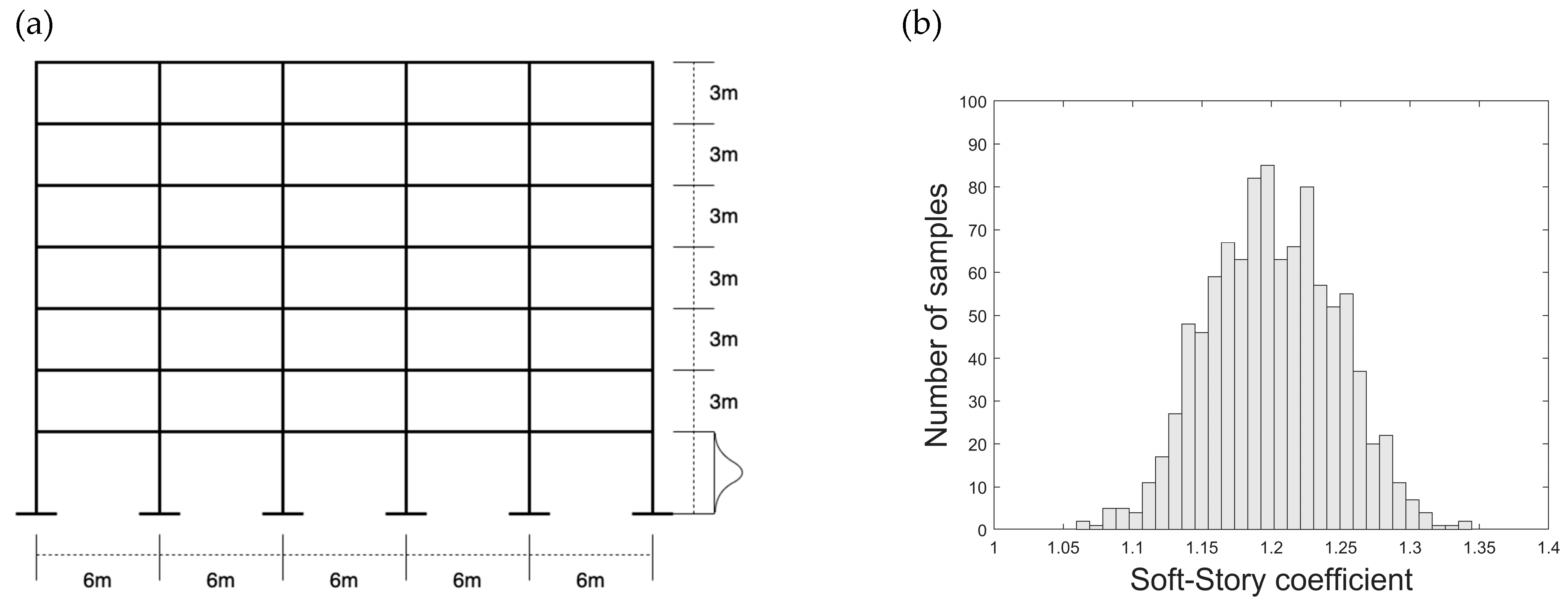
19,
20]. Most of these sources of uncertainty are not considered in this investigation, instead, a 2D seven-story building model has been used to perform the statistical analyses;
Figure 1a shows a sketch of this structure.
According to the above, for single structures, uncertainties in the gravity loads and mechanical properties of the materials become the most relevant [
21,
22]. Therefore, live loads,
LL, permanent loads,
DL, the compressive strength of the concrete,
fc, the tensile strength of the steel,
fy, and the elastic modulus of the concrete and steel,
Ec and
Es, respectively, have been considered as aleatory variables. Continuous Gaussian distributions have been assumed for them. The expected values employed, µ, standard deviations, σ, and coefficients of variation, σ/µ, according to [
23], are shown in
Table 1.
Regarding modelling considerations, the in-cycle behaviour of beams and columns has been represented by means of the modified Takeda hysteresis law, [
24]. This law allows including strength degradation because of large deformations and number of inelastic cycles [
25]. Moreover, the post-yielding branch is defined through a hardening coefficient equal to 5%. The α degrading factor has been fixed to 0.4 in order to account for stiffness degradation. The bending moment-axial load and bending moment-curvature interaction diagrams for columns and beams, respectively, define the yielding surfaces. Because of the large deformation expected in some simulations, P-Delta effects have been taken into account in the numerical model.
One-thousand realizations of the described building have been generated. It is worth mentioning that the first-story height of these models has been considered as a random variable. The objective is to take into account the influence of the soft-story (which is type of elevation irregularity), when analysing the seismic response of structures [
26]. In this way, a random Gaussian coefficient has been generated to multiply the height of the first story; mean and standard deviation are set to 1.2 and 0.045, respectively (see
Figure 1b).
It is worth mentioning that the cross section of the structural elements as well as the mechanical property values (
Table 1) have been selected to meet the behaviour of RC structures located in earthquake-prone areas in Europe. To verify this, the fundamental periods of the generated models are compared with the approximation given by the European seismic design regulations [
26]:
where
represents the fundamental period of the structure whilst
H its height.
Figure 2 compares the fundamental period of the generated models and those obtained by means of Equation (1). Note that since the first-story height statistically varies,
values estimated through Equation (1) become a random variable. However, the only source of uncertainty in Equation (1) is
H, explaining why the variability of the generated models, which is also affected by some of the variables presented in
Table 1, is much higher. In any case, similar mean values are observed in both distributions.
3. Seismic Hazard
In order to properly assess the seismic performance of the analysed structure, it is necessary to obtain an adequate set of ground motion records, which should be subsequently scaled at incremental intensity levels. Nevertheless, the limited number of strong ground motion records covering high-intensity intervals is a common impediment found in current databases [
27]; this may derive in excessive scaling to reach these intervals. In addition, scaling a single record to incremental intensity levels will generate false correlation between IMs and EDPs. To deal with these problems, the following steps have been employed for choosing and scaling ground motion records:
- (1)
Identify the database. The European strong motion database collected by the ‘Istituto Nazionale di Geofisica e Vulcanologia’, INGV, has been used to find appropriate ground motion records [
28]
- (2)
Identification of the IM to perform the selection and scaling of the records
- (3)
Calculate the IM identified in the previous step related to each ground motion record
- (4)
Categorize the ground motion records in descending order depending on the calculated IM values
- (5)
Define intervals of IM in descending order
- (6)
Define the number of records per interval ()
- (7)
The ground motion record ranked as first in the categorization (Step 4) is scaled to fall into the highest interval. If the IM naturally fulfil the interval condition, no scale factor is considered. This step is repeated until having records belonging to the highest interval
- (8)
The last step is repeated to have the desirable number of ground motion records () within each interval. The scale factor is calculated so that the IM values are uniformly distributed within the interval
In order to scale ground motion records with the purpose of this study, it seems reasonable to select an IM highly correlated to the structural response so that, by increasing the IM, the structural response would be expected to do so as well. Thus, it is more adequate to look into IMs calculated from the spectral response of single-degree-of-freedom systems, SDoF, as they have been shown to be highly correlated with the structural response. In this respect, several researchers have proven that is more efficient to use IMs based on average spectral values around the fundamental period of the structure than using the spectral value associated to it [
5,
6,
7,
8,
9]. However, because of the probabilistic features of the analysed structure, the fundamental period of the structural models varies (see
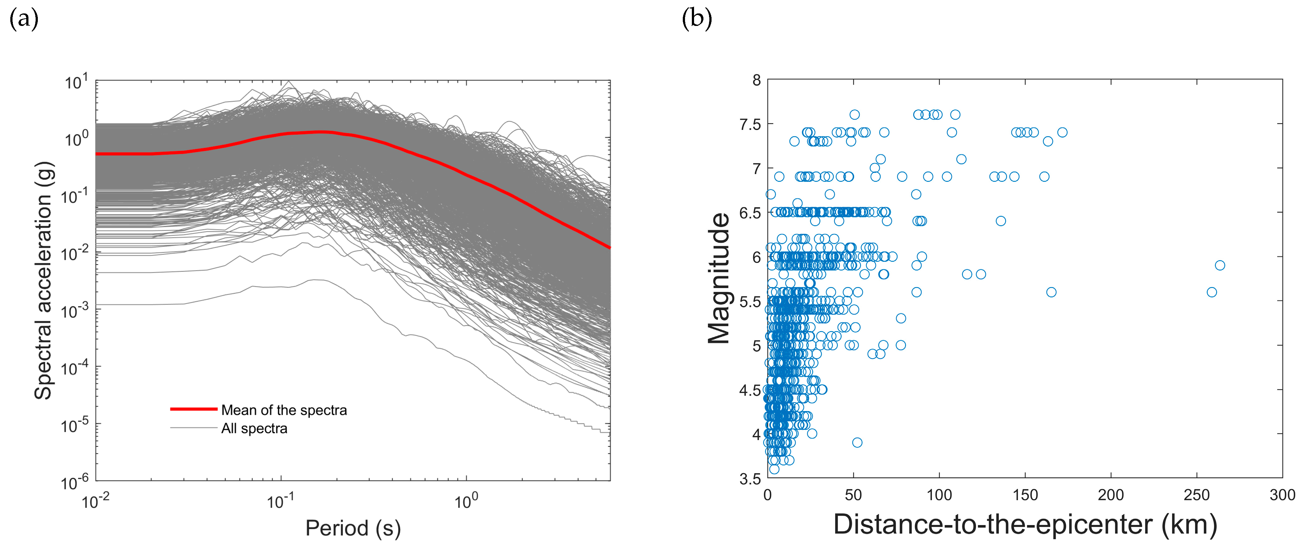
Figure 2). Hence, the period range for averaging the spectral ordinates of the IM is established from the dynamic properties of the building’s realizations. In this way, groups of ground motion records are selected whose mean spectral acceleration, in the period interval (0.07–1.26) s, lies in a band limited by two intensity levels. The intensity levels defining the extreme limits of each band range from 0.0 to 1.0 g at intervals of 0.1 g. One hundred ground motion records are considered for each band; in this way, as many records as models are selected.
Figure 3a presents the response spectra of the one-thousand records selected and scaled (if necessary) from the database.
It is also important to select ground motion records from different seismic sources in terms of seismological parameters (e.g., magnitude and distance-to-the-epicentre). Thus, the sufficiency property can be properly explored.
Figure 3b shows the magnitude and distance-to-the-epicentre distribution of the set of records.
Figure 4 presents a flowchart that summarizes the steps for selecting and scaling ground motion records described in this section
4. Intensity Measures and Engineering Demand Parameters
4.1. Intensity Measures
As starting point, three types of scalar-based IMs have been analysed in this article: (i) response-spectrum-based IMs; (ii) spectrum-energy-based IMs; and (iii) IMs based on direct computations from strong motion records. The first type is related to the dynamic response of several damped SDoF systems in front of the ground motion record; these IMs are usually extracted from the response spectra in acceleration, velocity or displacement. The second type, spectrum-energy-based IMs, are calculated from the equivalent elastic energy spectrum, which is associated with the energy introduced into a set of SDoFs by a ground motion. This function has received special attention since several researchers have proved its effectiveness in the prediction of the dynamic response of structures [
29,
30,
31,
32]. IMs of the third type can be obtained from calculations performed directly on the ground motion record; to this category belong IMs such as peak parameters (e.g., PGA). Note that this type of IM does not take into account the dynamic properties of structures.
A brief description on the three types of scalar-based IMs is presented in the following. As will be seen later, the vector arrays have been generated from this set.
4.2. Spectrum-Based Intensity Measures
The dynamic response of complex structures subjected to ground motions has been correlated to the maximum response of equivalent linear elastic damped SDoF systems. It has been observed that efficient IMs can be developed from response spectral ordinates. This explains why these measures are commonly used to represent seismic hazard at a site. Such ordinates are calculated from the solution of the dynamic equilibrium equation for SDoF systems:
where
,
and
contain the time-history evolution of the response in terms of acceleration, velocity and displacement, respectively;
is the ground motion acceleration (input);
m,
c, and
k are the mass, damping and stiffness of the system, respectively.
4.2.1. Spectral Acceleration-Based Intensity Measures
Spectral acceleration at the first-mode period has been probably the most used IM to characterize the seismic response of a structural system. This IM is obtained according to the following equation:
where
represents the critical damping fraction of the system; in this study,
has been set to 0.05 for estimating IMs. Analogous to
, it has been analyzed the statistical performance of
and
, which correspond to the spectral acceleration of the periods related to the second and third mode of vibration, respectively. Using these three IMs (
,
and
), and by considering the participation factor associated to the first three modes of the structure, the following IM has also been analysed:
where
is the participation factor associated to the mode of vibration
i of the structure.
In order to consider the participation of higher modes, and possible elongations of the first-mode period of the structure due to damage, an improved IM, which is based on the average spectral acceleration, has been widely studied [
5,
6,
7,
8,
9]. This IM, commonly known as
, is obtained as the geometric mean of spectral acceleration ordinates around the fundamental period. However, in this article, it has been considered more adequate to use the arithmetic mean rather than the geometric one since the variability between IM-EDP pairs tends to be lower [
33]. Thus, a modified average spectral acceleration IM,
AvSa, is obtained using the arithmetic mean of the spectral ordinates within a period range limited by β
inf ×
T1 and β
sup ×
T1. Vargas-Alzate et al. found that β
inf = 0.1 and β
sup = 1.8 are suitable coefficients to define these interval limits [
34]. Thus,
AvSa is estimated by means of the following equation:
where
represents the components of a vector that contains
period values equally spaced within the range 0.1 ×
T1 − 1.8 ×
T1, at intervals of 0.01 s.
Finally, an IM calculated as the maximum spectral acceleration in the range (0–6) s, named, has also been considered in the statistical analysis.
4.2.2. Spectral Velocity and Displacement-Based Intensity Measures
Another sets of IMs have been analysed herein, which are analogous to the previous one (
Section 4.2.1) but calculated from the velocity and displacement response spectra. That is, the same IMs presented in
Section 4.2.1 have been obtained by using the velocity and displacement spectra instead of the acceleration one. It is worth noting that several IMs extracted from these spectra have been recognized to be very efficient in previous research [
35,
36,
37,
38].
4.3. Energy-Based Intensity Measures
The design or assessment of civil structures have been strongly tied to physical magnitudes like displacement, velocity or acceleration. However, several researchers have presented evidence on the efficient relationship between expected damage and the amount of energy introduced into the structure [
29,
30,
31,
32]. In this respect, the equivalent velocity spectrum is a graphical representation that has been used to quantify the amount of energy introduced into a set of SDoF models. This energy can be calculated by rewriting Equation (4) in terms of energy (see Equation (6)) [
39,
40]:
For the sake of convenience, the time dependence of acceleration, velocity and displacement responses have been omitted in this equation;
is the kinetic energy;
is the energy dissipated by the inherent damping;
is the energy absorbed by the system; and
is the energy introduced into the system by the ground motion. From this term, the equivalent velocity,
, is obtained as follows:
The equivalent velocity spectrum is obtained by calculating
VE for several elastic oscillators;
Figure 5 shows these spectra for the records described in
Section 3.
4.3.1. Equivalent Velocity at the First-Mode Period
From the
VE spectra presented in
Figure 5, the equivalent velocity at the first-mode period of the structure,
, can be obtained as follows:
4.3.2. Average Equivalent Velocity
Analogously to IMs based on average spectral values, it is proposed to analyse the behaviour of the average spectral equivalent velocity,
, which can be obtained by means of the following equation:
4.4. IMs Based on Direct Computations of the Ground Motion Records
In this section, a set of IMs that are obtained from computations of the ground motion record are presented. The attractiveness of these IMs is their independence from the dynamic properties of the structures. Several of these IMs are described below.
4.4.1. Peak Ground Acceleration
One of the first instrumental IMs of strong ground motion intensity was the peak ground acceleration, PGA, [
41]. For a specific accelerogram, this IM is obtained as the maximum acceleration occurred at the recording station using the following equation:
4.4.2. Peak Ground Velocity
The peak ground velocity, PGV, is calculated from the ground motion record in terms of velocity. This IM tends to be highly correlated with the building response. For instance, Wald et al. [
42] found that PGV correlates Modified Mercalli Intensity better than PGA. Alike to PGA, PGV can be obtained as follows:
4.4.3. Peak Ground Displacement
The maximum displacement occurring at a site due to an earthquake, Peak Ground Displacement (PGD), has practical applications in earthquake early warning systems [
43]. Particularly, this IM has been used to estimate the event size in earthquake early warning applications [
44]. Since this IM is strongly sensitive to the baseline offset, special attention should be drawn to the baseline correction of the record [
45]. The PGD can be calculated using the following equation:
4.4.4. Arias Intensity
The Arias intensity [
46] is an IM addressed to estimate the severity of a ground motion and it is defined by the following equation:
where
g is the acceleration due to gravity;
ti and
tf correspond, respectively, to the beginning and end of the acceleration signal. Based on the Arias Intensity, Trifunac and Brady [
47] defined the significant duration of a ground motion, Δ, as the time interval where 5% and 95% of Arias intensity are achieved, that is: Δ =
−
. These limits are adopted in this research to obtain Arias intensity and some of the subsequent IMs (i.e.,
and
)
4.4.5. Root-Mean Square Acceleration
Housner [
48] suggested that the ground motion can be characterized by the quadratic mean of the acceleration time history, also known as root mean square acceleration,
, which is defined as follows:
Recall that Δ is the significant duration as defined above.
4.4.6. Root-Mean Square Velocity
The root-mean square of the velocity time history,
, has been associated with damage in several studies [
49,
50]. This IM can be estimated as follows:
4.4.7. Specific Energy Density
Another interesting IM is the Specific Energy Density, SED, [
51,
52]. This IM is defined as the integral of the square velocity time-history (see Equation (16)).
4.4.8. Cumulative Absolute Velocity
The Cumulative Absolute Velocity (
CAV) was proposed by Reed and Kassawara [
53] and it has also been used to state the destructive potential of ground motions induced by earthquakes:
4.4.9. Characteristic Intensity, IC
Park et al. [
53] developed an IM considering the relationship between the destructiveness potential of a strong ground motion and the structural damage of reinforced concrete buildings. These authors used the damage index proposed by Park and Ang [
54] as EDP. Thus, the characteristic intensity,
IC, is obtained as the product of a ‘scalar’ IM,
, and the duration of the acceleration record,
, in the form of power functions (see Equation (18). In order to be consistent with the time limits considered for previous IMs,
has been replaced by Δ:
4.4.10. PGV-Duration Intensity,
Recently, Pinzon et al. [
18] revisited the improved IM proposed by Fajfar et al. [
17], which is obtained as the product of a scalar IM, PGV, and the significant duration, Δ, in the form of power functions. Pinzón et al. [
18] and Fajfar et al. [
17] found that this power arrangement would produce an improved IM able to predict efficiently the seismic response of buildings. This IM can be estimated by means of the following equation:
Pinzón et al. [
18] found that for steel frame moment resistant structures, whose number of stories range from 3–13,
and
. Fajfar et al. [
17] proposed that, for structures with fundamental periods in the medium-period range,
and
. This fact shows that depending on the fundamental period of the systems, the participation of the significant duration is variable within the power arrangement.
4.5. Engineering Demand Parameters
4.5.1. Maximum Global Drift Ratio (MGDR)
This EDP is used for determining the general performance of structures when subjected to ground motion records. MGDR can be obtained by dividing the maximum displacement at the roof,
, between the height of the building:
In the case of NLDA,
is estimated as follows:
where
represents the time-history displacement at the roof of the building
4.5.2. Maximum Inter-Story Drift Ratio (MIDR)
The MIDR is probably the most used EDP when analysing the seismic performance of buildings [
55]. Specifically, this variable is used to control the design or assessing the vulnerability of buildings. For a story
i, the evolution of the inter-story drift is given by:
where
is the time-history displacement at the floor
i of the building;
is the height of the story
i. Thus, the maximum inter-story drift ratio at the story
i,
, can be calculated as follows:
Finally, the maximum inter-story drift ratio in the building, MIDR, is given by:
4.5.3. Maximum Floor Acceleration (MFA)
The Maximum Floor Acceleration,
MFA, is an
EDP highly associated to damage in non-structural components [
56]. It can be calculated by analysing the time-history response of each floor in terms of acceleration.
where
is the time-history acceleration at the floor
i of the structure. Thus, in order to estimate non-structural damage, the
MFA observed in the building is given by
where
is number of floors of the structure.
4.5.4. Base Shear Coefficient (
In order to quantify the acting force transmitted to the foundation, the base shear coefficient is calculated by dividing the maximum base shear by the total weight of the building,
W:
where
represents the time-history response of the base shear.
5. Statistical Analysis of IM-EDP Pairs
The nonlinear dynamic analysis (NLDA) is the most reliable numerical tool to simulate the seismic response of buildings. Accordingly, this has been the type of structural analysis employed herein. The Ruaumoko software has been used to perform these calculations [
25]. In this manner, one-thousand NLDAs have been performed.
It has been found a number of simulations indicating structural collapse. These outcomes are classified as those having an MIDR higher than 4%. In addition, simulations in which PGA > 1.5 g, PGV > 3 m/s, PGD > 1 m or Sa(T1 > 4 g have been also excluded from the statistical analyses. Thus, 881 (≈88%) out of the one-thousand generated samples meet the requirements described above. From this number, 146 are elastic results whilst 735 are inelastic ones. According to this classification, the resulting clouds of IM-EDP points are used to perform the statistical analysis.
As commented above, one of the most desirable features in IMs is efficiency in predicting EDPs. In summary, an IM is efficient if it reduces the dispersion when estimating EDPs. In this respect, multi-regression systems can be used to identify the best combination of IMs to explain an EDP. Therefore, both multi-linear and -nonlinear regression models in the log-log space have been used to characterize IM-EDP relationships.
In brief, nonlinear regression is based on obtaining a set of values able to minimize the sum of the squares of the residuals. Hence, the general linear least-square model can be adapted to predict EDPs in the log-log space as follows:
where
represents the number of IMs considered in the regression model;
n is the polynomial degree of the model;
,
, …
are the coefficients providing the best fit between model and data;
represents the residuals. Note that Equation (28) allows regression analysis considering any polynomial degree. Therefore, information coming from several IMs can be combined to enhance the prediction of a specific EDP. Numerical details on the development and implementation of polynomial regression models in the log-log space can be found in [
57]. Thus, for
= 1 Equation (28) adopts the following form:
There are several options to quantify the variability (in terms of
) of IM-EDP clouds. For instance, Ebrahimian et al. [
37] considered the logarithmic standard deviation of the regression,
, and the correlation coefficient,
. It is worth mentioning that the higher
or the lower
, the lower the variability when predicting some EDP given an IM. Both variables have been employed in this research to quantify variability.
As commented above, linear and quadratic regression models, i.e.,
n = 1 and
n = 2 in Equation (29), respectively, have been compared. The reason for considering a higher polynomial order is that several IM-EDP pairs exhibit a non-linear dependence in the log-log space. In fact, the use of linear regression, when characterizing these pairs, have been called into question, e.g., [
11]. Hence, some authors proposed that consecutive piecewise linear relationships can be fitted, e.g., [
58]. In this research, it has been opted to fit a quadratic regression model. Note that when an IM-EDP set of points indicates a linear tendency, the quadratic model automatically makes the nonlinear term close to zero (i.e.,
in Equation (29).
In order to differentiate statistical properties coming from linear or quadratic regression models (i.e., n = 1 and n = 2 in Equation (29), respectively), a subscript indicating the degree of the polynomial has been considered for and . Thus, for a linear regression type, these two terms are and ; and for a quadratic type they are and .
In the following, variables described in
Section 4 are used as IMs and EDPs.
and
have been calculated considering three approaches: (i) using only elastic results; (ii) using only inelastic results; (iii) using both elastic and inelastic results.
5.1. Elastic Range
As mentioned above, a number of building models remained within the elastic range. These results have been identified as those having a damage index of Park and Ang equal to 0 [
55].
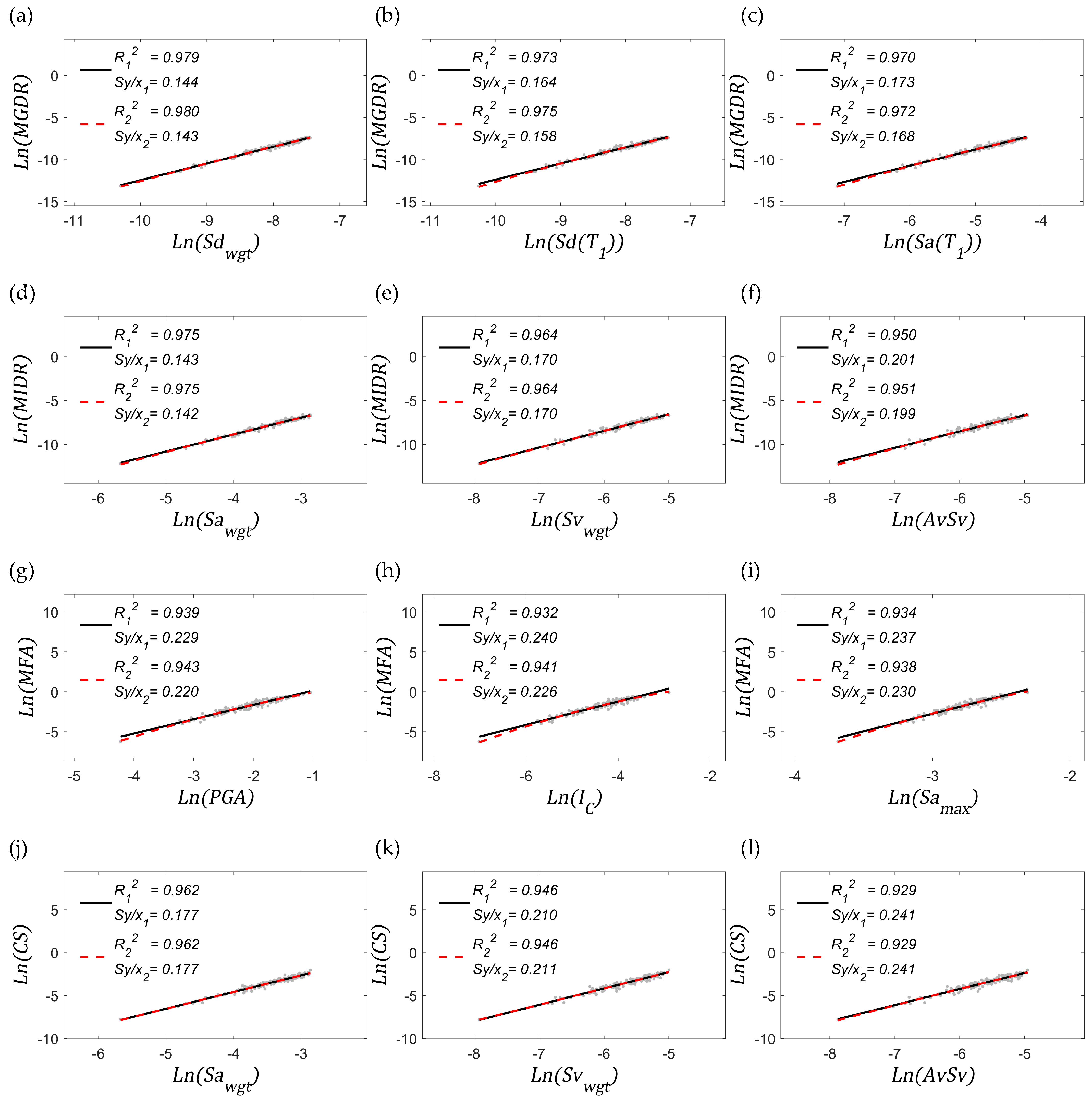
Figure 6 shows the relationships in the log-log space between all the EDPs described in
Section 4.5 and the three most efficient IMs, considering only results in the elastic range. IMs have been ranked in descending order based on
values, starting from the most correlated one. In
Appendix A, the results for the entire set of IMs are presented.
In general, it can be observed that linear and quadratic regression models provide similar scattering values. In other words, it has not been observed a significant variation of the dispersion when using any of these models. The most significant difference can be appreciated when the EDP is MFA; actually, the regression lines based on the quadratic approach become slightly different from the linear case. From
Figure 6, it can be concluded that the most efficient IM varies depending on the analysed EDP. However, high-efficiency values are observed for all cases. It is also important to note that IMs based on weighted spectral values (those with the subscript wgt) generally exhibit the highest efficiency. In terms of physical magnitudes, if the EDP is MFA, acceleration-based IMs tend to exhibit the highest efficiency. For the rest of EDPs, it cannot be stated a dominant physical magnitude.
Regarding sufficiency with respect to magnitude, most of the IMs presented in
Figure 6 meet this property, i.e., the p-values between residuals and magnitude are higher than 0.05; only the relationship
-MFA does not meet the sufficiency condition. In terms of the distance-to-the-epicentre, all the IMs presented in this figure are sufficient.
5.2. Inelastic Range
Most of the simulations performed in this study fell within the nonlinear range.
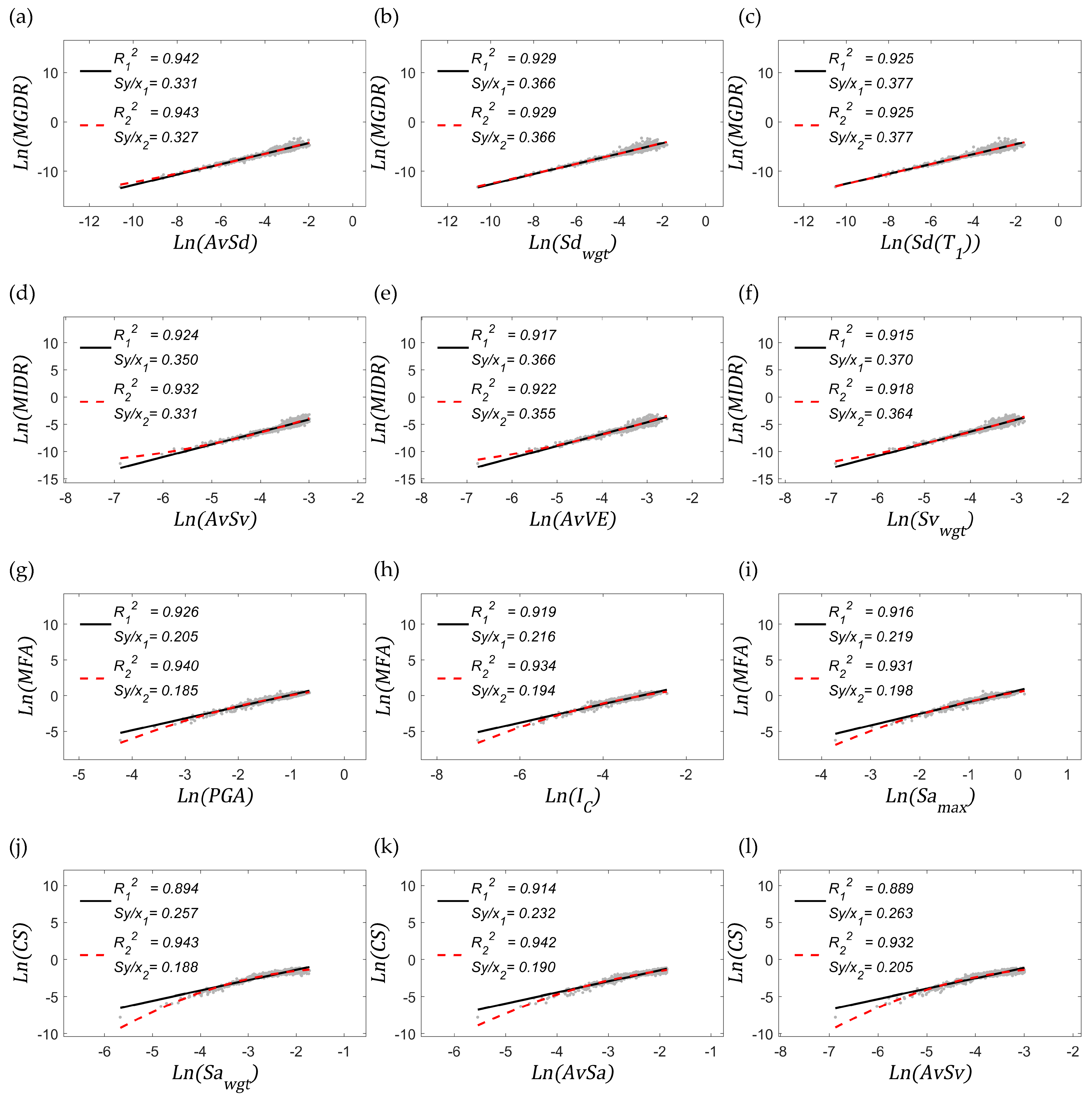
Figure 7 shows the relationships between all the EDPs and the most efficient IMs according to this classification. This figure also shows a general decay of the efficiency when compared to the elastic results; this is to be expected as the complexity of the dynamic response in the nonlinear domain increases. However, several IMs remain at a significant level of correlation. It can be also seen that the linear regression model fits reasonably well most of the IM-EDPs relationships presented in
Figure 7.
In terms of the MGDR, spectral displacement-based IMs are the most efficient ones. Note that, as in the elastic case, is highly correlated with this EDP. Regarding MIDR, those related to velocity and to equivalent velocity spectrum are the ones with the highest explanation capacity; the IM most correlated with the MIDR is AvSv. For MFA, it can be seen that acceleration-based IMs are the most efficient ones, as in the elastic case; again, PGA is the best proxy.
Note also that
is still a highly correlated IM. In the case of CS, spectral acceleration-based IMs are the ones exhibiting the highest efficiency. However, AvSv appears on the podium. Note that this IM has been identified as the one exhibiting the most stable efficiency for predicting several of the EDPs analysed herein [
35]. In general, it is noteworthy that average spectral-based IMs are the ones with the highest explanation capacity in the inelastic range for most of the EDPs analysed.
Regarding sufficiency with respect to magnitude, it has been observed that most of the IMs do not meet this property. Only the residuals of MGDR-AvSd, MFA- and MFA- present p-values higher than 0.05. In terms of the distance-to-the-epicentre, similar conclusions can be drawn. However, the three most correlated MGDR-EDP pairs stand out since they meet the sufficiency requirement. Also, the residuals of MFA-PGA pairs exhibits a p-value higher than 0.05. From this analysis it can be concluded that the sufficiency requirement is more difficult to achieve when considering inelastic results.
5.3. Overall Range (Elastic and Inelastic)
A-priori, it is not possible to establish with certainty whether a structure will experience deformation beyond the elastic range given a ground motion. For this reason, it has been analysed what occurs with
and
when the efficiency is measured joining the results in both domains, i.e., elastic and inelastic. Note that most of the methodologies to estimate seismic risk consider results of both cases. Therefore,
Figure 8 shows these relationships in the log-log space. Again, the most three efficient IMs are presented.
The main conclusion of mixing elastic and inelastic results is that, except for MGDR, the EDPs analysed are better fitted by the quadratic regression model than the linear one. This can be observed after comparing and (or and ). In terms of the efficiency analysis, similar conclusions can be drawn from the inelastic results. For instance, the podium remains identical in both cases for MGDR and MIDR. For MFA and CS, although the position of the most correlated IMs is not identical, almost the same IMs appear in the set (except for which is substituted by ).
After analysing the sufficiency exhibited by the IMs in the combined case, it has been observed that, with respect to magnitude, only two cloud of pairs exhibit this statistical property; they are MGDR-AvSd and MFA-. In terms of the distance-to-the-epicenter, again, the three most efficient IMs to predict MGDR are sufficient; so are MFA- and CS-AvSa. In general, the sufficiency analysis shows that this property is easier to achieve if the seismological parameter is the distance-to-the-epicentre.
According to the results presented in this section, it has been observed that scalar IMs are more efficient to predict MGDR and MIDR rather than MFA and CS. Anyhow, significant levels of correlation are observed, which are particularly high for the elastic case. However, the most correlated IMs tend to be no sufficient with respect to seismological parameters, especially for inelastic results. In the next section, it will be shown how to identify more efficient vector-valued IMs, which meet the sufficiency condition.
6. Enhancing Statistical Properties by Combining Pairs of IMs
In annex A, it can be observed that the efficiency of two basic IMs (
and PGV) increases when combined with the significant duration,
. This outcome gave rise to two improved IMs, named
[
54] and
[
56,
57] (also discussed in this article). According to this, it would be of interest to analyse if new improved IMs can be developed by combining pairs of scalar IMs (i.e.,
= 2 in (1). In doing so, (1) adopts the following form:
By means of this enhanced arrangement, it has been analysed the efficiency of all the possible pairs of combinations of the scalar IMs described in
Section 4. Consequently, 435 vector-valued IMs have been analysed.
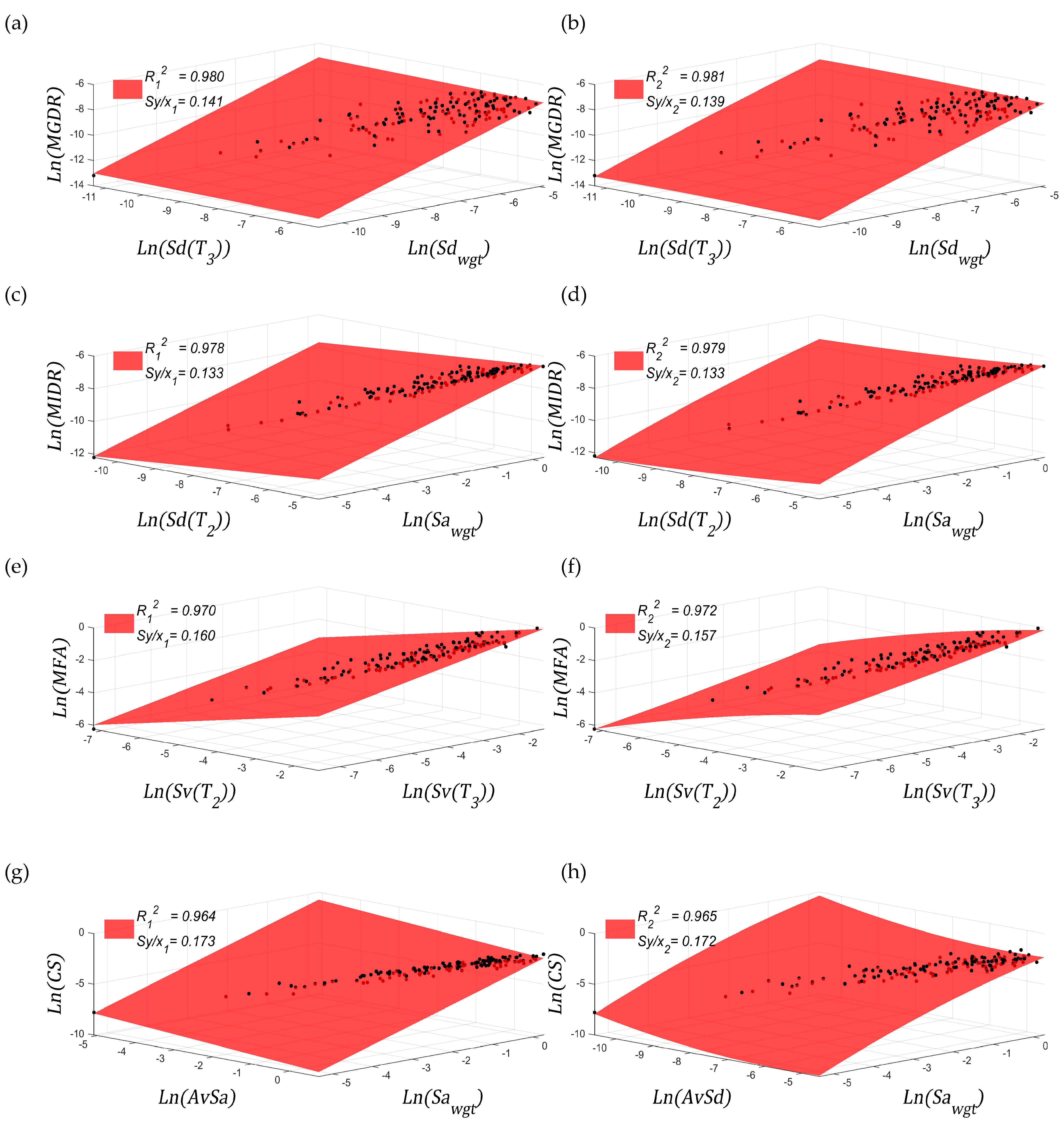
Figure 9 presents the pairs of IMs most correlated with all the EDPs by considering elastic results.
In
Figure 9, it has been compared results coming from a linear (Left) and a quadratic (Right) regression analysis (Recall that (1) allows multi-linear (
n = 1) and -quadratic (
n = 2) regression models in the log-log space). Note that in terms of efficiency, the only case in which can be appreciated a significant increase of this property is for MFA (this EDP showed the lowest level of correlation when analysing scalar IMs). It is also important to observe that, except for MFA, the scalar IMs identified as the most correlated (i.e.,
= 1) also appear in the vector arrangement.
Regarding sufficiency, all the presented combinations meet this statistical condition with respect to magnitude and distance-to-the-epicentre. This outcome is expected since most of the scalar IMs exhibiting the highest efficiency met the sufficiency condition (at least for elastic results).
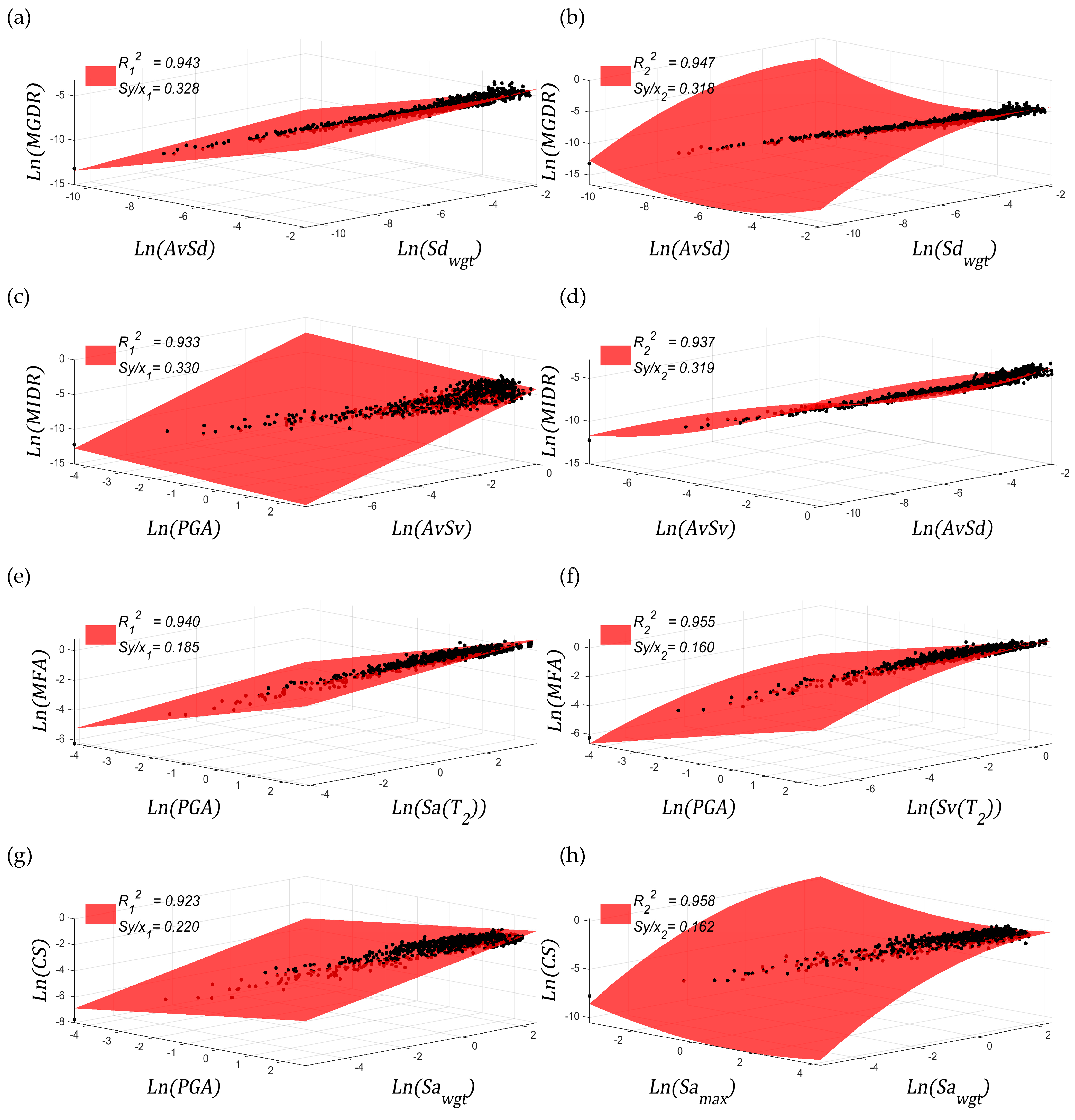
Figure 10 presents the regressions for the inelastic data. Again, linear (Left) and quadratic (Right) regression models have been employed. In this case, for all the EDPs, the scalar IMs identified as the most correlated ones also appear in the vector arrangement.
In terms of efficiency, no significant changes have been observed for MIDR and MGDR; for MFA and CS, an increase of this property has been detected, being more pronounced for CS. Regarding sufficiency, all the vector arrangements shown meet this condition, proving thus the enhanced statistical properties of these IMs. Note that, when analysing single IMs, the sufficiency condition was rarely fulfilled by the most correlated IMs, especially for inelastic results.
Figure 11 shows the regression results for both elastic and inelastic data. As in the inelastic analysis, the most correlated IMs identified in the scalar case also appear in the vector arrangement. However, only for MFA, it has been observed a significant increment of the efficiency. Anyhow, causality is more evident in vector arrangements than in scalars ones. In terms of sufficiency, all the presented arrangements have demonstrated independence of both seismological parameters, i.e., magnitude and distance-to-the-epicentre. This shows that the vector-valued IMs are better proxies to estimate the EDPs analysed in this research than the scalar-based ones.
7. Conclusions
In most engineering problems uncertainties prevail. The most followed approach to address this randomness is to identify what characteristic of the input(s), or a combination of them, maximizes causality with an output of interest, so that reliability increases. This helps decision-makers to operate with confidence.
In several methodologies to quantify seismic risk, input variables related to hazard are characterized by means of IMs. Output variables are characterized from the dynamic response of the analysed structure (EDPs). This article has been oriented to obtain sets of input-output variables (IM-EDP) whose causality relationship is maximum. To do so, a set of scalar IMs have been analysed, with the purpose of identifying the most efficient ones. A seven-story reinforced concrete building has been used as a testbed. The structural analysis employed to perform the calculations has been the NLDA.
The scalar IMs selected depend on physical magnitudes like displacement, velocity, acceleration and energy. Regarding EDPs, the ones calculated are function of the deformation field of the structure (MGDR and MIDR), the acceleration response (MFA), and the acting forces (CS). One of the main conclusion of this analysis is that, depending on the EDP analysed, the most efficient IM may vary. It has been observed that MGDR is well explained by displacement-based IMs; MIDR by velocity-based ones; MFA and CS by acceleration-based IMs.
The statistical analyses have been performed by separating results in elastic, inelastic and a combination of both. From this classification, it has been observed that the most efficient IMs may also vary. In addition, two types or polynomial regression models have been considered (i.e., n = 1 and n = 2 in (1). The main conclusion is that, when combining elastic and inelastic analysis, the regression based on the quadratic polynomial approach is more efficient than the linear one to predict EDPs.
In addition to causality (Efficiency), for the sake of convenience, other statistical properties have been desired in IMs [
4]. One of the most pursued have been sufficiency. In summary, this property is related to the invariability of the regression results when the selected ground motion records come from different types of seismic sources. Specifically, the sufficiency has been measured with respect to the magnitude and distance-to-the-epicentre. It has been found that, when considering inelastic data, this statistical feature is barely accomplished by the most correlated IMs. Nonetheless, in the case of elastic results, most of the IMs that present high efficiency are sufficient with respect to the seismological parameters (magnitude and distance-to-the-epicentre).
In order to increase efficiency, and to tackle the generalized lack of sufficiency of scalar IMs, it has been proposed to develop vector-valued IMs by combining pairs of the scalar-based ones. Thus, 435 possible vector arrays have been created and their efficiency to predict EDPs has been measured. Efficiency has always been found to increase, although it is more notorious when considering MFA. This trend is observed for all types of results (i.e., elastic, inelastic or a combination of both). This increase in efficiency makes it possible to reduce the number of structural calculations, which is significant considering the elevated computational effort involved in the NLDA.
As commented above, because of the seismological diversity of the selected ground motion records selected in this research, the sufficiency property is barely met when considering scalar-based IMs. However, when performing multi-linear and –nonlinear regression models, this property is accomplished by several of the enhanced arrangements (vector-valued set). To get an idea of how important this conclusion is, note that, the most efficient, which is also sufficient, scalar IM to predict MIDR has an
= 0.888 and
= 0.425. For this EDP, a vector-valued IM meeting both statistical conditions has an
= 0.933 and
= 0.330. Note that, efficiency and sufficiency properties maybe affected by the seismological parameters of the selected ground motions. For instance, if a distinction is made between near- and far-fault records before performing statistical analyses [
59,
60], the efficiency is expected to increase when compared to that calculated for the entire dataset. In terms of sufficiency, this classification makes that a higher number of scalar IMs meet this property.
Future research should be oriented to verify if the conclusions extracted from the current research apply to other structural typologies e.g., [
61,
62,
63] or seismological environments. It is also of interest to verify how these arrays behave when considering 3D models. Anyhow, this article provides an idea on the enhanced capabilities of IMs when multi-regression models are applied in the statistical analysis.


