1. Introduction
Structure health monitoring (SHM) [
1] consists in the stability monitoring of man-made structures such as buildings, highways, and bridges, that suffer from deterioration, aging, inadequate upkeep or earthquake damage. Monitoring civil infrastructure allows to detect the deformation at an early stage, preventing risks and keeping public safety and quality of life. Timely inspections of civil infrastructures usually involve human resources, in situ contact sensor, and considerable funds. Contact sensors are characterized by high sensitivity and can monitor the most critical points of the constructions, detecting factors that may be symptoms of poor structural health, such as anomalous displacements. Temperature structure monitoring and the resultant strain and displacement is another structural health tool (Temperature Driven-Structural Health Monitoring or TD-SHM) [
2,
3]. Changes in the signatures that describe the structure’s behavior with temperature indicate unusual behavior or damage. A fundamental parameter for this analysis is the Coefficient of Thermal Expansion (CTE), which is the amount of expansion or contraction a material undergoes per degree change in temperature.
A solution for the routine inspections of civil infrastructures with reduced human resources and affordable costs is based on remote sensing systems, such as synthetic aperture radar (SAR), that offer the possibility for large area and millimeter-level surface deformation monitoring under all day and during all weather conditions [
4,
5].
In particular, synthetic aperture radar interferometry (InSAR) is a cost-effective methodology for measuring surface deformation over large areas [
3,
4,
5,
6]. By applying multi-temporal InSAR processing techniques, (for example Persistent Scatterers PS InSAR) [
7,
8,
9,
10] to a series of SAR images acquired during time over the same region, it is possible to detect the line of sight (LOS) movements of ground and of civil infrastructures, and to evaluate the average velocity of their movements with a millimeter sensitivity. Therefore, it is possible to detect anomalous movements indicating potential stability structure problems that require further ground investigations. An early problem detection allows to mitigate their impact on structural health. Different sensors can be used for frequently monitoring a specific area of interest. For instance, ERS, Envisat, and Radarsat have monthly revisit time, while Sentinel, TerraSAR-X, and COSMO-SkyMed provide even weekly revisit time [
11,
12]. Moreover, it is also possible to map deformations which occurred in the past, if images of the site were acquired. Several studies have highlighted the potential of PS InSAR techniques in estimating the displacement of civil structures and of their thermally induced displacement that exhibits a seasonal behavior [
13]. PS InSAR techniques are essentially phase model-based and assume the presence of one dominant scatterer within a resolution cell [
7,
8,
9,
10,
11,
12,
13]: the deformation is measured only over the available coherent pixels. The deformation model usually cannot be assumed linear, especially in the case of civil structures, such as bridges, railways, and specific buildings with metallic cover, whose construction materials may be sensitive to thermal dilation effects. In this case, due to the temperature changes, the structure may undergo large non-linear seasonal deformations [
14]. In general, the interferometric phase is modeled as the sum of deformation, thermal dilation effect, and noise terms. In order to measure the deformation contribution, which is independent of temperature variations, the estimation of the thermal dilation contribution is crucial [
15,
16]. Recently, based on conventional InSAR, various time-series InSAR techniques have been developed, aimed at mapping and characterizing the thermal dilation of different infrastructure types [
17,
18,
19]. The magnitude of thermal dilation is proven to be highly variable for each infrastructure since it is associated with the material properties and sizes of the objects [
19]. In general, it achieves values of the order of millimeter. The capability to measure thermal dilation contribution is related to sensor sensitivity, in particular, sensors in X-Band, such as TerraSAR-X and the Italian COSMO-Skymed constellation, characterized by a very small wavelength (~3.1 cm), allows to measure small surface displacements, even those caused by thermal dilation of the imaged targets.
Even if PS InSAR techniques are widely used in this field, they undergo two-fold limitations when monitoring specific structures in urban areas: on one side, the phase unwrapping operation [
4] (the complex-valued phase interferogram is modulo 2π and must be unwrapped) in correspondence of many height discontinuities can be inaccurate, and, on the other side, the assumption of only single scatterer in the resolution cell cannot allow to consider the layover problem [
20]. Layover is a geometric distortion present inside the looking radar: in the illuminated scene, the echoes from multiple scatterers at different height, but at the same slant range, are summed up, and contribute to the same resolution cell, ending up in a brighter area in the SAR image. This phenomenon can impair the selection of PS and the corresponding height and displacement estimation.
This limitation can be overcome using SAR tomography (TomoSAR) [
20,
21,
22] where scatterers interfering within the same range-azimuth resolution cell are separated by synthesizing apertures along the elevation direction. In study [
21], it has been shown that the number of scatterers detected using TomoSAR is higher than that identified by PS-InSAR. In structure health monitoring, a higher detected point density allows, on one side, to better identify the critical points that need to be monitored, and on the other side, to infer with more accuracy potential damage for the structure monitored if the point cloud exhibits the same anomalous deformation behavior. The higher scatterer density in the TomoSAR case is due to the coherent processing of the complex valued data (amplitude and phase) in the elevation direction, that allows to increase the signal to clutter ratio in the focused 3D domain. InSAR techniques, instead, are based on only-phase data. Moreover, in TomoSAR, the estimation of the scatterers’ parameters is performed by simultaneously exploiting all the acquisitions, thus allowing an optimal smoothing of the phase noise and of the additive clutter effect, with a subsequent increase of the estimation accuracy.
TomoSAR is still based on a stack of SAR images acquired at different times but considers both amplitude and phase of the acquired signals and allows to provide the full 3D scene reflectivity profile along azimuth, range, and elevation. Moreover, it does not require the phase unwrapping but mainly consists in resolving a spectral estimation problem. Different spectral estimators have been proposed, such as Singular Value Decomposition (SVD) [
23] and Compressive Sensing (CS) [
24,
25,
26].
TomoSAR techniques derive the elevation and deformation parameters of multiple scatterers present in each resolution cell, together with noise contributions and artifacts that can be misinterpreted as scatterers. One of the main issues that must be faced is the correct detection of true scatterers in presence of noise and outliers. This problem can be treated by fixing the maximum number of scatterers that can be present in each resolution cell and using a detector [
27], based on a statistical model of the data, capable of detecting the presence of scatterers and estimating their number. The detector proposed in [
27] is based on a sequential Generalized Likelihood Ratio Test (GLRT), which allows to detect the presence of single and double scatterers, controlling the number of outliers with an assigned false alarm rate. The detection performance depends also on the number of measurements and on the signal to noise ratio (SNR).
In study [
28,
29,
30], different GLRT approaches have been proposed, achieving super resolution capabilities. This is a very important issue in urban structures monitoring for discriminating scatterers which are very close in elevation, such as those coming from the building roof, façade and ground, or from different height buildings in the same illuminated area.
Extended phase models [
31,
32,
33,
34,
35] have been introduced to allow simultaneous retrieval of scatterer elevation (3D map) and of deformation parameters, with the generation of a 4D map, by adding the velocity deformation contribution [
33], and 5D map, adding the thermal dilation effect [
34].
The Multi-look GLRT (MGLRT) [
36] has been introduced for the detection and monitoring of weak scatterers at close-to-full resolution in urban areas. It achieves an improved detection efficiency of PSs with constant false alarm rates compared with single-look GLRT approaches [
28,
29].
In this paper, the results obtained by using the MGLRT TomoSAR technique based on the extended phase model [
36,
37], in order to retrieve the 5D reconstruction of buildings in urban areas, are presented. Multi-looking operation essentially involves an averaging operation on the signals acquired in a given neighborhood of each range-azimuth image pixel, for reducing the noise effect and improving the result accuracy. Anyway, two considerations have to be made:
the averaging operation produces a reduction of the range and azimuth resolutions, which can impair the reconstruction of small and medium-sized structures;
for achieving a good performance, the averaging operation has to be performed over an area that is spatially stationary (without elevation changes), otherwise it can lead to results that are worse than the ones obtained in the single-look case.
It follows that for structure monitoring in urban areas, where a high spatial resolution is required, and the observed scene is not spatially stationary, a multi-looking operation has to involve a very small number of pixels.
Results on real TerraSAR-X (TSX) data are presented in order to investigate if TomoSAR techniques can be used for assessing both possible deformations and thermal dilation evolution of man-made structures. The results obtained using X-band SAR data in two case studies, concerning two urban structures in the city of Naples (Italy), are presented.
To sum up, the main contributions of the paper are:
Showing the potential of TomoSAR as a structure health monitoring technique:
on real TSX data, starting from unfiltered single-look complex SAR images;
on small-size urban infrastructure, where it is crucial to detect, as much as possible, scatterers providing reliable results.
Showing the impact of neglecting the thermal dilation contribution that can impair height and deformation estimation, with a consequence on the right localization and on the detection of anomalous movement of the critical points on the structures.
2. Materials and Methods
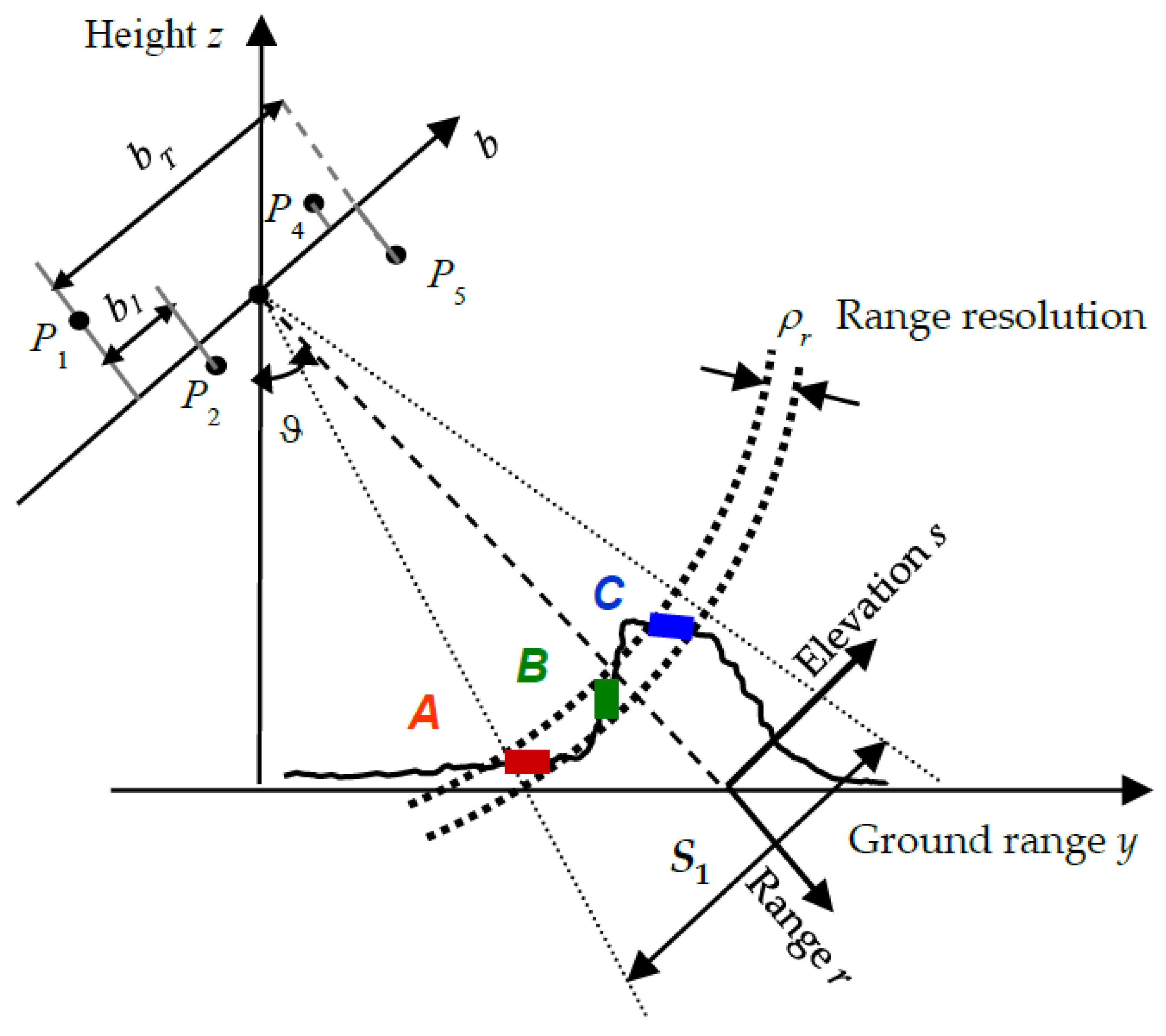
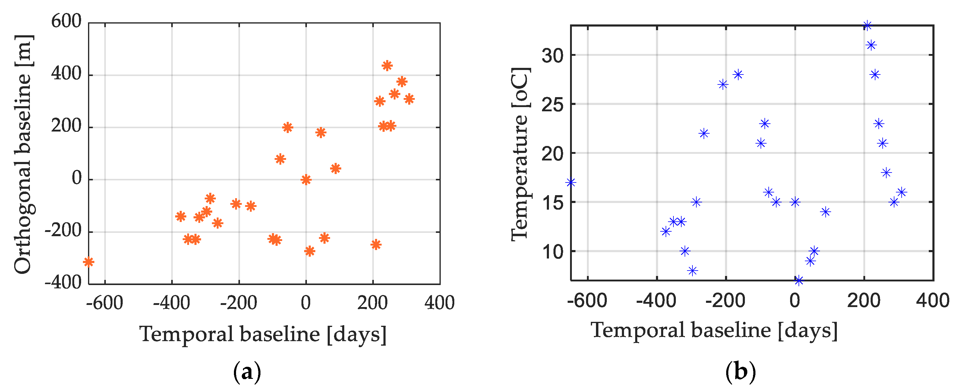
TomoSAR is a technique that exploits a stack of
M SAR interferometric images of the same scene, as shown in
Figure 1, where the acquisition geometry is shown in the
rs-plane obtained by fixing the
x coordinate, where
x,
r, and
s are the azimuth, slant range, and azimuth coordinates, respectively. The images are acquired at different times
tm and with different orthogonal baselines
bm in respect to a reference acquisition. The images are firstly co-registered in order to spatially align them, then flat Earth interferometric phase is removed, and pre-processing is carried out to depurate the focused images from the atmospheric and nonlinear deformation contributions on a small scale (low resolution) [
28]. Then, in each azimuth-slant range cell (
x–r), the
m-th acquired image
um is given by the superposition of the signal backscattered by the targets located in the given
x–r resolution cell at different elevation value
s s and with reflectivity
g(
s). Then, the image signal, in the case of slow-moving scatterers can be expressed by [
31,
34]:
where
l is the operating wavelength,
R0 the distance between the image pixel and the reference antenna, and
S1 the extension of the observed scene along elevation (see
Figure 1).
The phase term in Equation (1) is given by the sum of the first term, that depends on the scatterer elevation,
s, and, of the LOS deformation displacement of the scatterer at the elevation
s and at the time
tm,
d(
s,
tm). The LOS deformation term can be modeled considering a linear and a nonlinear contribution: a slow linear contribution, in time, with a mean velocity, that models a linear land subsidence phenomenon; a nonlinear contribution in time but linear in temperature, that models the material thermal dilation, and a limited nonlinear contribution that is neglected. Following these assumptions, the LOS deformation [
31,
34] is:
where
Tm is the temperature of the scene at the time
tm,
v(
s) is the mean velocity of the slow linear deformation, having the dimension of (m/sec), and
k(
s) is the coefficient of thermal dilation, having the dimension of (m/°C), of the scatterer at elevation
s, representing the phase to temperature sensitivity, and depending upon material and/or physical structure.
Typically, as reported in the Introduction, the thermal deformation component is of the order of mm/°C and can be estimated thanks to the X-Band sensors, that allow a higher phase sensitivity to range variations with respect to other C or L-Band sensors.
The coefficient of thermal dilation
k in Equation (2) is given by
k = Δ
L/Δ
T, where Δ
L is the change in length of the solid structure due to a change in temperature Δ
T. It is related to the Coefficient of linear Thermal Expansion (CTE) α of the solid structure, that represents the percentage variation in length per degree of temperature (m/(m·°C)), by the relation
k =
α L0, where
L0 is the initial length of the given solid [
38].
We note that in Equation (2), a simple thermal expansion model, linear with temperature, has been assumed; indeed, the civil structures are not thermally uniform, and undergo a more complex thermally induced displacement that depends on the geometry, the construction material, and the temperatures across the entire structure. A more sophisticated model will certainly ensure better thermal dilation estimates, but this is not the aim of the paper. We aim to show the potential of a TomoSAR technique in the field of civil structure monitoring and the need to include the thermal expansion in the adopted phase model. Even considering a linear model, the inclusion of the thermal contribution allows to achieve more accurate height and deformation estimates.
In the case of urban areas, most of the elevation profiles are sparse, i.e., they consist only of a few discrete scatterers, for instance, in
Figure 1, three contributions (A, B, C) in the same (
r–x) cell are considered. In this paper, we focalize on structures to be monitored and on high reliable points positioned on them; for this reason, we search for a dominant coherent scatterer in each (
r–
x) cell, but applying a TomoSAR technique, we exploit both amplitude and phase signals and avoid the unwrapping operation, which can be critical when observing areas with highly discontinuous height profiles, as happens in urban areas.
Discretizing Equation (1), we can assume a signal model in two different hypotheses: presence of a target (H
1) or absence of a target (H
0):
with
where
g is the reflectivity coefficient of the dominant coherent scatterer present in the
r–x cell at the elevation
s, exhibiting deformation velocity
v and thermal dilation
k,
w(
bm) is the additive clutter and noise contribution to the
m-th acquisition, and
a(
s,
v,
k) is the steering vector. Note that, after the above mentioned flat Earth removal operation, the elevation
s is related to the height
z by the relation
z =
s sin(
θ), where
θ is the look angle introduced in
Figure 1, so that the steering vector in Equation (4) is depending on look angle.
The presence of one scatterer can be verified by performing a statistical test. In Equation (3), the noise vector
w can be assumed as circularly symmetric complex (or proper complex) Gaussian vector, with uncorrelated samples and mutually uncorrelated real and imaginary parts, with zero-mean and same variance
σ2. The probability density functions under the two hypotheses are both Gaussian, under H
1,
depends on the target parameters (
γ,
s,
v,
k) and on the noise variance
σ2, while under H
0,
depends only on the noise variance
σ2. The two hypotheses can be identified applying a Generalized Likelihood Ratio Test (GLRT) [
29]:
The threshold η is set using a Constant False Alarm Rate approach, which consists in imposing a false alarm rate equal to an assigned value, and evaluating the corresponding threshold by means of Monte Carlo simulation. A sample size of realizations (the size should be chosen in accordance with the fixed rate) of noise signals, i.e., the data under hypothesis H0 is generated, and the threshold is evaluated such that the GLRT is over the threshold with the fixed false alarm rate.
The expression of the Maximum Likelihood estimates of
γ and
σ2 maximizing Equation (5) can be found in a closed form. Consequently, after some mathematical manipulations, a simplified form of the test is obtained [
36,
37]:
The detector in Equation (6) exhibits performance, in terms of detection capabilities (for an assigned false alarm rate) and in terms of parameter estimation accuracy, that depends on the number of acquisitions
M, on the scatterer coherence among the
M acquisitions, and on the Signal to Noise Ratio (SNR). In practice, the performance can be unsatisfactory when
M is too small [
36,
37]. Hence, to improve the performance achieved with a fixed false alarm, contextual information can improve the detector performance. For each considered pixel of the image, a patch of
L pixels, typically a window of
N × N pixels, with
L =
N2 can be considered, so that the number of data exploited to detect the scatterer and estimate the corresponding parameters (
s,
v,
k) is increased of a factor
L. A common assumption, if
N is limited, consists in assuming that the pixels belonging to the same patch exhibit the same target parameters, so that the test becomes a Multi-look test (MGLRT) [
36,
37]:
In this paper, the Test (7) is applied to recover the 5D reconstruction of the illuminated scene; where the target is present, it provides a reliable estimate of elevation, deformation velocity, and thermal expansion coefficient. The accuracy of the parameters’ estimates is related to the scatterers’ intensity and to their coherence over time: the higher the scatterer intensity and the temporal coherence, the more accurate the parameter estimation. The pixel neighborhood dimension
L, for consideration in Test (7) is selected based on a compromise between estimation accuracy and the compliance of the assumption that all
L pixels share the same parameter values. In this paper, a neighborhood with
L = 9, considering 3 × 3
r–x cells for each pixel has been chosen (see [
37] for details).
The procedure followed by MGLRT for the detection of a single scatterer is reported in
Table 1:
In
Table 1, the sets
S,
V, and
K represent the range values for the triplet (
s,
v,
k), and the initialization is done considering a search grid for each parameter, compatible with the illuminated scene and the considered phenomena. For instance, in urban areas, where skyscrapers are present, the maximum elevation can be set to 150 m, the thermal dilation parameter depends on the material and can be set, at most, to 1 or 2 mm/°C, and the deformation average velocity can be set, at most, to 1 or 2 cm/year. The maximization in step 5 consists in an exhaustive search of the entire parameters’ space.
4. Results and Discussion
Two different urban test sites in Naples (Italy) were considered:
- (1)
an area around the Galleria Umberto I, which is a high and spacious cross-shaped structure, surmounted by a glass dome braced by 16 metal ribs, height 57 m, with four iron and glass-vaulted wings, maximum length 147 m, width 15 m, height 34.5 m;
- (2)
an area around the Jolly Hotel, which is one of the tallest buildings in Naples, made of reinforced concrete, height 100 m, with a telecommunications tower on the top.
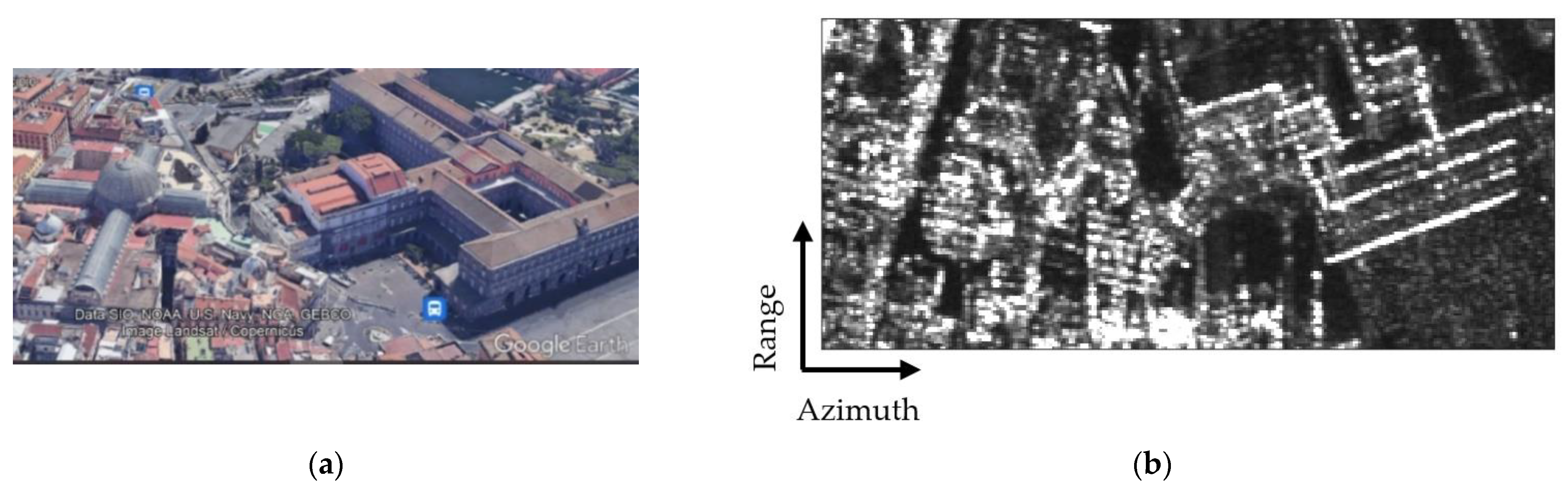
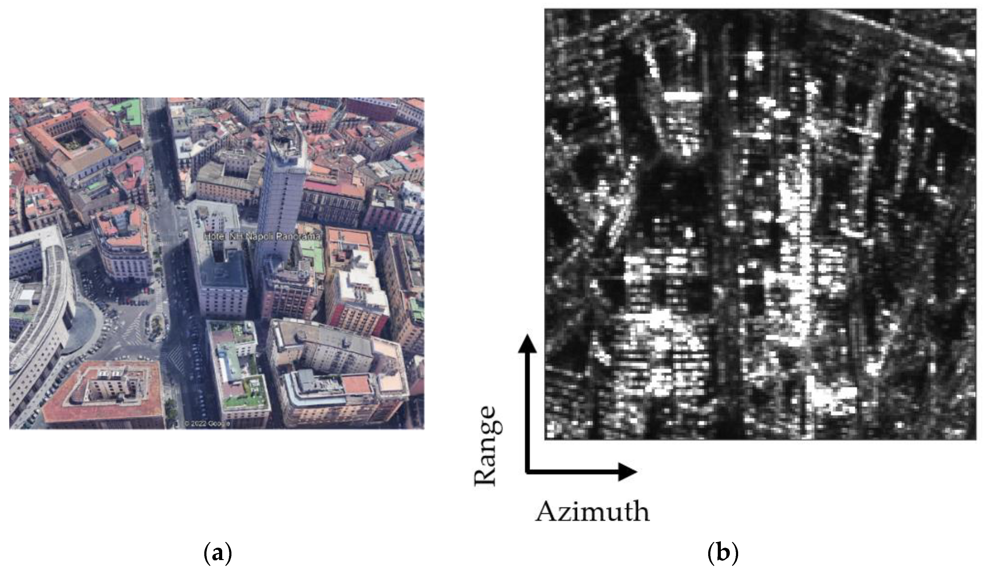
Figure 3 refers to the first site and shows the optical and SAR images of Galleria Umberto I and its neighborhood. The first thing to be noted is that a SAR image (
Figure 3b) needs processing and interpretation for structure monitoring. In fact, SAR images undergo well-known geometric distortions, such as shadowing and layover [
4], which are related to the slanted imaging coordinate system of the SAR sensor, causing the points at higher elevations to appear in the image at smaller range values. The layover effect will clearly appear in the reconstructed height maps, but can be easily compensated after height estimation, by means of the geocoding operation.
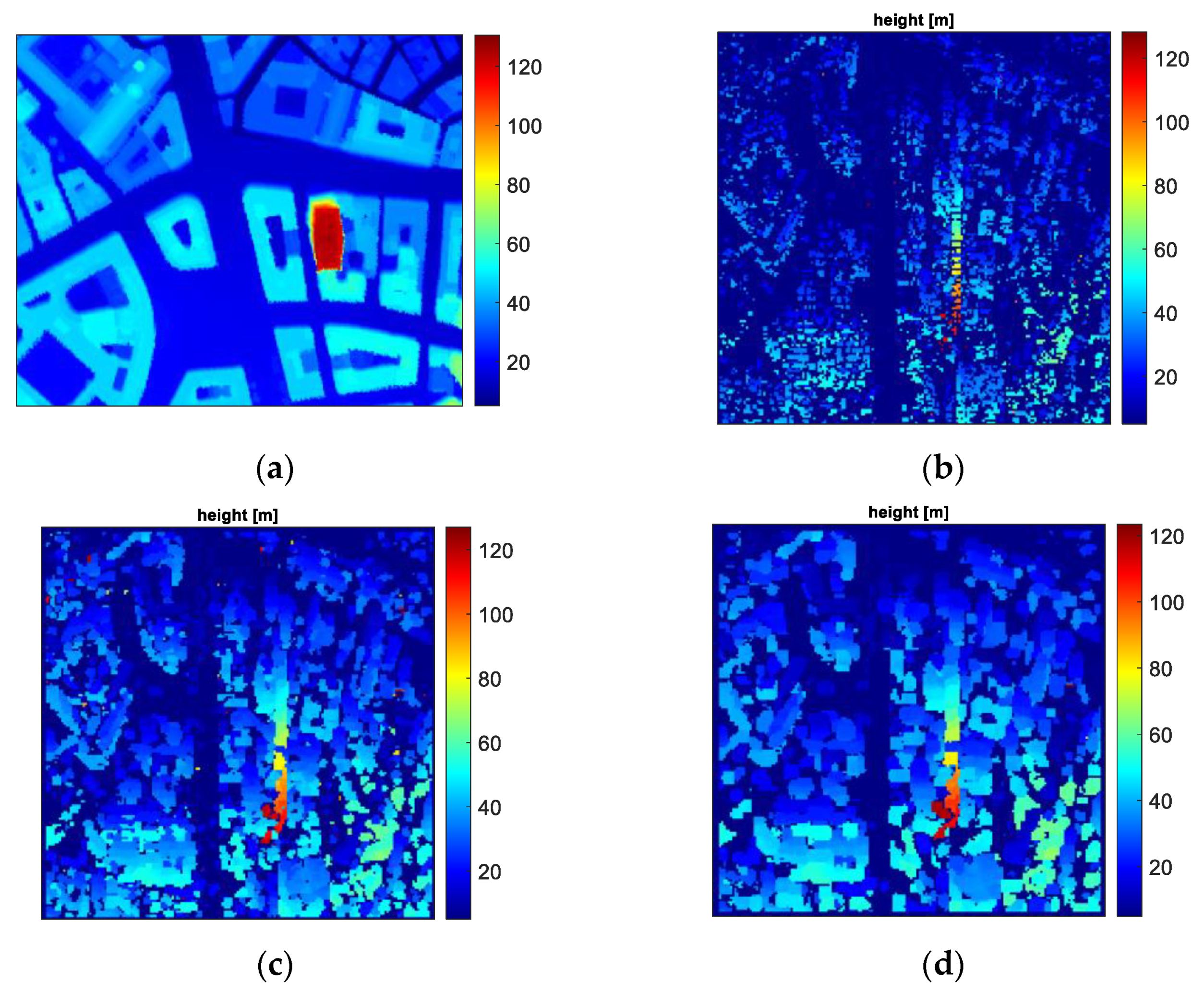
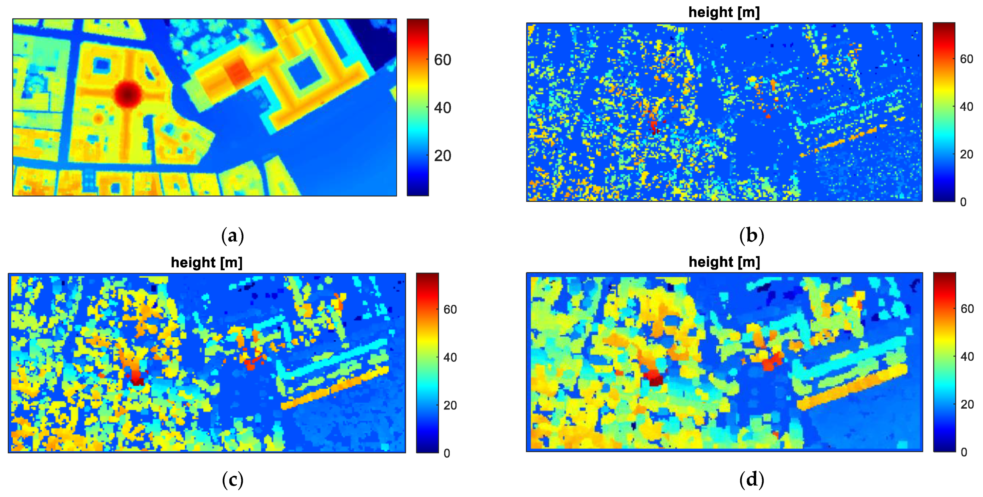
In
Figure 4a–d, the LiDAR ground truth (a) and the height maps of the test site estimated using single-look GLRT (b) and MGLRT using 3 × 3 (c) and 5 × 5 (d) patches are presented. In the maps, only the height values of the scatterers with a value of
greater than the fixed threshold (see Equation (7)) are shown. It can be easily noted that when increasing the patch size, the reconstructed height maps are more dense and less noisy, but spatial resolution decreases and some details are lost. A good compromise between scatterers’ density and resolution is given by the results obtained using the 3 × 3 patch. In
Figure 4b–d, we can also notice the phenomenon of layover, causing the point with high elevations to be located at lower range values. The reconstructed height map exhibits a satisfactory accuracy when compared with the LiDAR map (
Figure 4a). For instance, the height of the dome is well estimated as ca. 60 m.
In
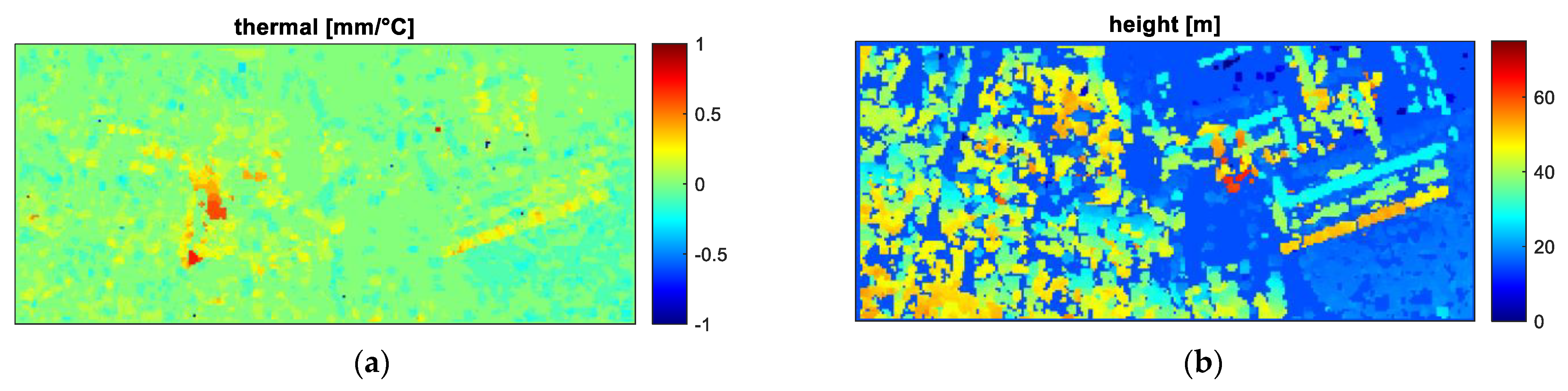
Figure 5a, the MGLRT thermal dilation map which was obtained by applying a 3 × 3 patch is shown. In this map, a significant thermal dilation is present on the iron and glass dome and vaulted wings, as expected. In
Figure 5b, MGLRT estimated a height map obtained without including thermal dilation and by applying a 3 × 3 patch is shown. By comparing the height map obtained in this case with the LiDAR one (
Figure 4a) and with the one obtained by considering the thermal dilation (
Figure 4c), it appears evident that this map is less accurate than the one obtained taking into account thermal dilation. In fact, in
Figure 5b, the dome is not any more visible with its 60 m height. This behavior proves the importance of including this deformation component in the signal model.
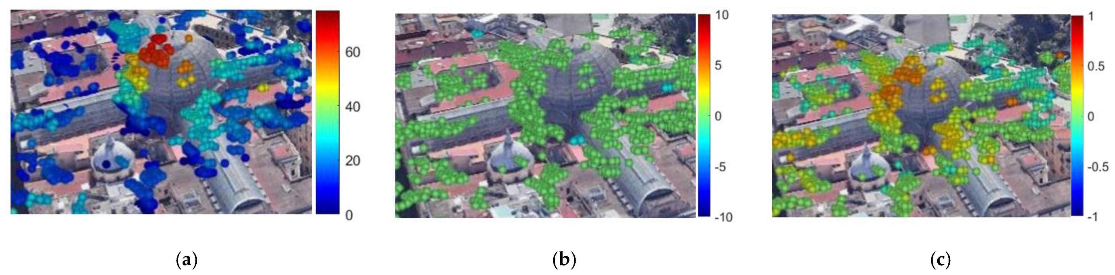
In
Figure 6a–c, the points were detected using MGLRT with a 3 × 3 patch, located in the optical 3D image, with a colorization corresponding to the height (a), to the deformation velocity (b), and to the thermal dilation coefficient (c) which are presented. A negligible deformation velocity can be appreciated, while thermal dilation coefficient is not negligible and is increasing with the height, as expected.
The thermal dilation map shows a positive trend with height. Positive values of the estimated thermal dilation coefficient indicate that a positive temperature difference produced a displacement toward the sensor. Construction materials expand when the temperature increases, and this expansion is greater along the longest side of the geometric shape of the considered structure. This justifies why we estimate a greater thermal dilation coefficient on the top of the dome. The maximum thermal coefficient observed on the dome top is about 0.8 mm/°C. The computation of the thermal expansion coefficient is complex, due to the geometry of the dome; as reported in
Section 2, it takes into account the percentage change in structure length, per degree of temperature change. The obtained result shows that the maximum thermal dilation coefficient estimated is of the order of magnitude of the thermal coefficient of iron (about 12 × 10
−6 (m/(m·°C)); in fact, considering the maximum height of the dome (57 m), the thermal expansion is about 8 × 10
−4/57 = 14 × 10
−6 (m/(m·°C).
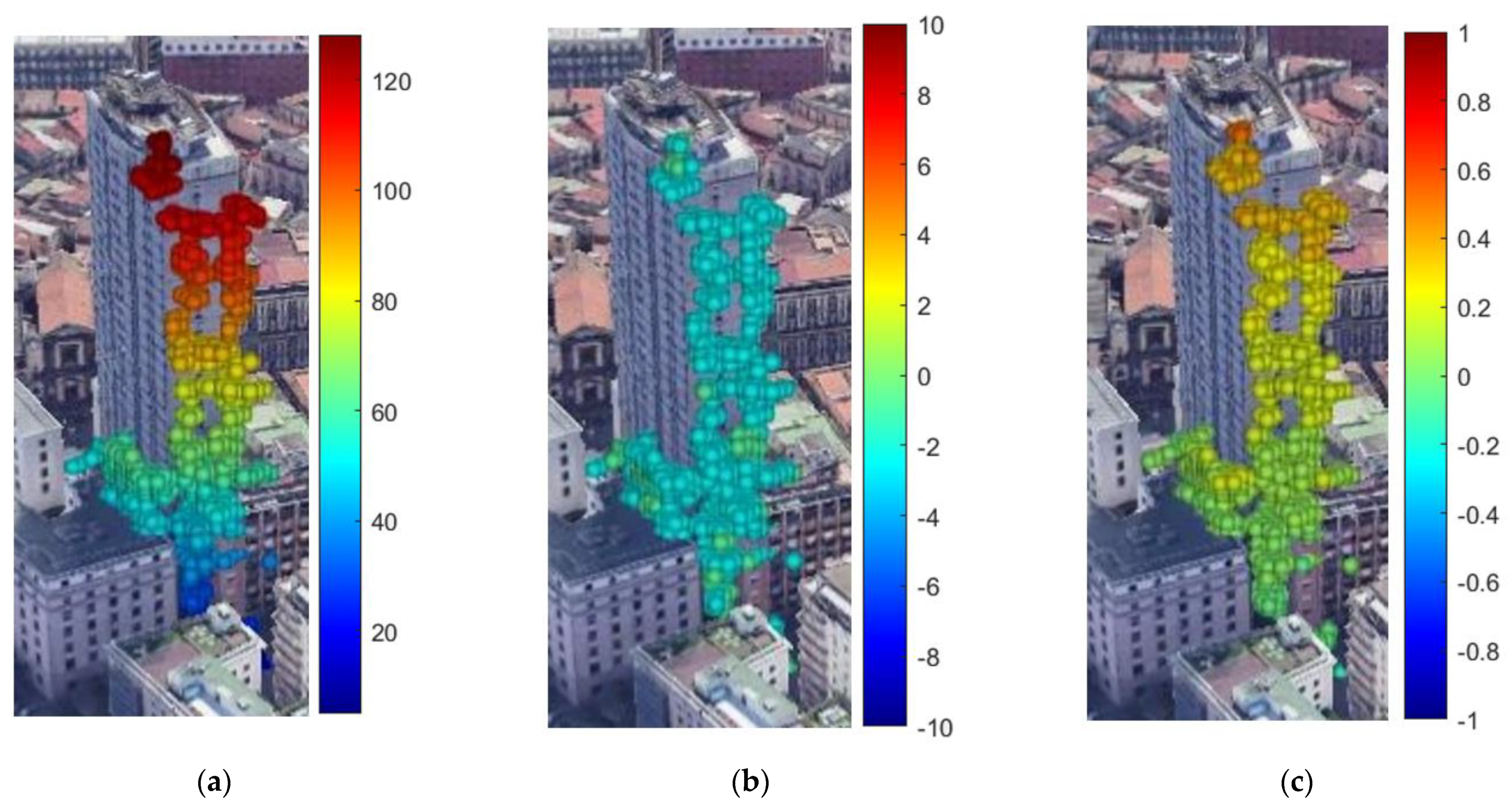
Figure 7 refers to the second test site and shows the optical and SAR images of Jolly Hotel and its neighborhood. Since this building is very tall (about 100 m), the layover effect is quite visible. In
Figure 8a–d, the LiDAR ground truth (a) and the height maps of the test site estimated using single-look GLRT (b) and MGLRT using 3 × 3 (c) and 5 × 5 (d) patches are presented. Additionally, in this case, the 3 × 3 patch represents a good compromise between resolution and accuracy. In
Figure 8b–d, the layover effect is quite evident, since the top of the tall building corresponds in the SAR image and in the corresponding height map to a smaller slant range than that of its bottom. Moreover, the height of the building is well estimated at about 100 m.
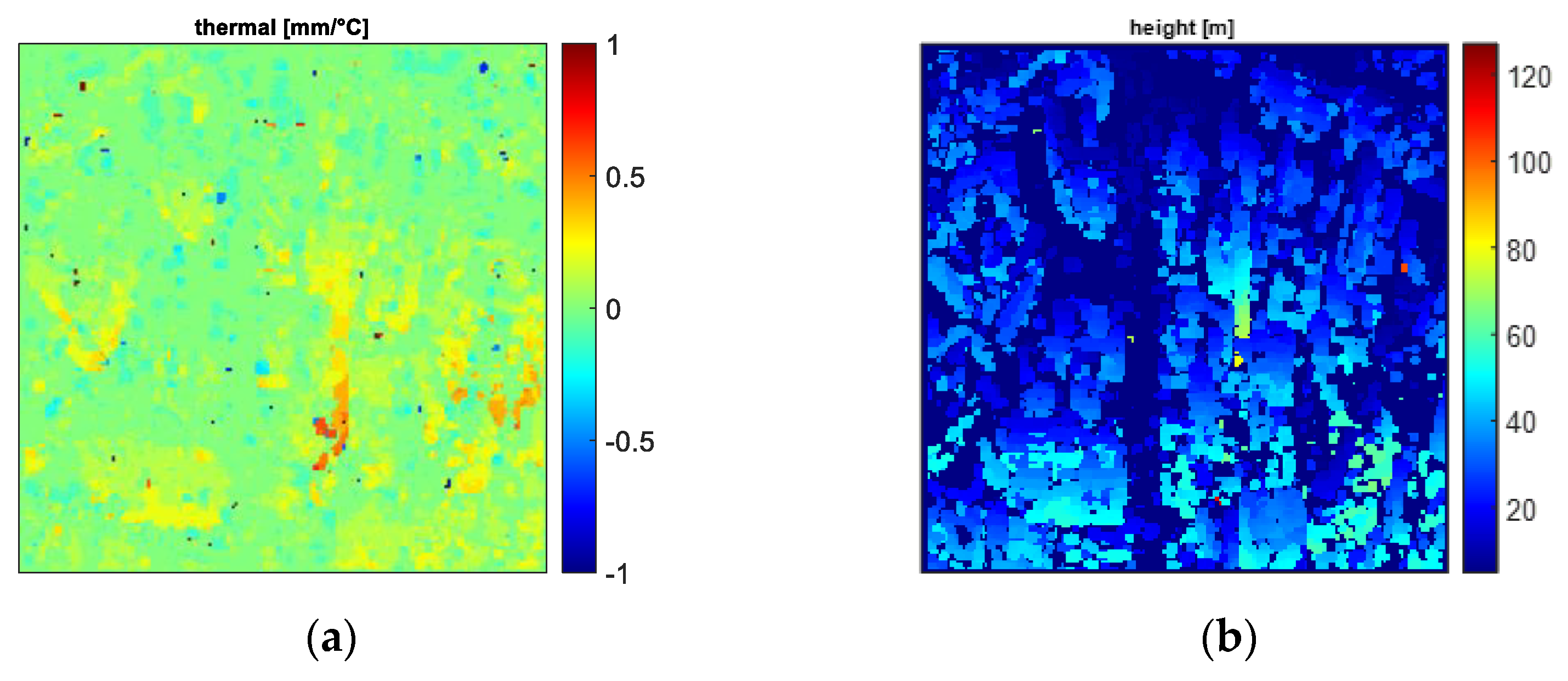
In this experiment, again, no linear deformation velocity has been detected, but the thermal dilation effect is visible in the map shown in
Figure 9a. It is very clear in
Figure 9b that without considering the thermal contribution, the height reconstruction fails, since the top of the building is not visible. Then, it is not possible to find critical points on the top for monitoring the structure. Finally, we show the detected cloud points relocated on the structure in the optical 3D image in
Figure 10. Again, a positive thermal dilation coefficient increasing with the height, as expected, is reported in
Figure 10b. The maximum thermal expansion that is observed on the top is about 0.9 mm/°C, so that, considering the building height of 100 m, the thermal expansion is about 9 × 10
−4/100 = 9 × 10
−6 m/(m·°C), which is compatible with the thermal expansion coefficient of the concrete (about 10 × 10
−6 (m/(m·°C)).
The results presented demonstrate that the adopted TomoSAR technique applied on TSX data exhibits a good capability of computing the height profile of structures on the ground and allows the estimation of their deformations on a sub-centimeter scale, separating thermal dilation from other kinds of temporal deformations.
5. Conclusions
In this paper, we show that SAR tomography can be a useful technique for civil structure health monitoring. A stack of SAR images of the structure under monitoring acquired during the observation period are needed, but the cost would be significantly lower than that of in situ contact sensors and ground investigation. The choice of the sensor depends on the availability of the data, but also on the systems characteristics required, such as revisiting time, spatial resolution, and wavelength, which is related to the sensor sensitivity and consequently, to the spatial scale of the movements that need to be monitored.
A Multi-look GLRT-based SAR tomographic technique has been applied. It exploits context information, processing image patches instead of pixel by pixel, achieving a better estimation accuracy. The adopted approach is able to estimate the height and two components of temporal displacements at a millimeter scale: a deformation component linear with time, which is usually related to presence of subsidence and structural damages, and a displacement component linear with the temperature, which is related to the thermal dilation effect of solid structures.
It has been shown that if the thermal dilation contribution is not taken into account in the model and not estimated, the assumption of the only linear deformation contribution can lead to not reliable estimates of the structure height and corresponding possible deformation. We note that this achievement has been reached considering an X-band SAR system (high sensitivity), and assuming for the thermal contribution the simplest possible model, linear with temperature. Of course, a more sophisticated model will certainly ensure better thermal dilation estimates, but the investigation of a more complex model is beyond the aim of the paper.
Applying the detection test, the more reliable points can be identified by means of a fixed constant false alarm criterion, and the estimated displacements on these points can be, then, usefully employed for the structure health monitoring. The high scatterers’ density obtained is due to the coherent processing in the elevation direction, typical of TomoSAR and not performed in InSAR techniques. The proposed approach allows to increase the signal to clutter ratio in the focused 3D domain also thanks to the multi-looking procedure.
In the numerical experiments, it has been discussed the dimension of the patch that should be considered for the multi-looking; the experiments on real TSX data have proven that a 3 × 3 is a good choice with a slight loss in resolution but a gain in accuracy. The only assumption that has to be done about the monitored structure is that the resolution of SAR system is such that the structure size is compatible with the chosen patch.
Finally, it should be highlighted that the presented work aims to show the potential of a TomoSAR approach in SHM, focusing on the scatterers’ density and the reliability of the parameters’ estimates (height, thermal dilation, deformation), but it is still not ready for being utilized by the industry. Limitations are the simple thermal dilation model, as discussed, and the lack of a consolidated procedure that helps the user to detect an anomalous behavior that can candidate a structure as a potentially damaged one, a type of damage index.


