1. Introduction
Digital Image Correlation (DIC) applications have been widely accepted and used recently, owing to the development of optical-based tools such as digital cameras and smartphones. Likewise, the advancements in computational photography accompanied by the rapid enhancement of the computational capabilities of the computers have also added to making the DIC a reliable and robust metrological tool adopted by multiple fields. However, as it is an optical-based technique, the DIC also suffers several shortcomings, such as the data variability delivered by correlation algorithms. Deformation variations are instigated by the ambient light noise impinging over the camera sensor. It is worth noting that these random errors produced by light noise are different from other sources of errors, such as camera vibration or heating. Moreover, the poor application of speckles to the material hampers realizing good correlation features.
In the literature, Bruck et al. 1989 [
1] suggested the image averaging procedure to eliminate random error from the random noise affecting the camera sensor. To assess these random errors, the author created an image averaged from 20 frames recorded over two minutes and compared it with a regular image within the Newton–Raphson DIC correlation algorithm framework [
1]. Later, Pan 2013 [
2] proposed a pre-processing approach based on “pre-smoothing” of the speckles using a five-by-five Gaussian filter to reduce the correlation bias error. The suggested technique minimized the measured displacement bias error to a negligible degree using only a bicubic interpolation algorithm [
2]. Also, Pan et al. [
3,
4,
5] suggested several experimental approaches in 2012, 2013, and 2014. Firstly, Pan et al., 2012 [
3] implemented an active imaging DIC approach using a monochromatic light filter over the camera lens. The active imaging approach applies a customized light illumination with a particular wavelength over the targeted surface. Then, images are captured for DIC analysis using a camera capped with a monochromatic light filter of a similar wavelength to the used artificial light. This technique provided images with a high-fidelity measurement as the camera sensor is not influenced by the ambient light variation of the environment. The active imaging approach showed promising potential for in-field DIC applications [
3]. Pan et al., 2013 [
4] used bilateral telecentric lenses for 2D-DIC to minimize errors produced by out-of-plane camera movement and camera overheating. The DIC was applied for a simple uniaxial tensile test of an aluminum sample together with traditional strain gages attached to the sample. The results from the DIC reveal that using a bilateral telecentric lens effectively eliminated the out-of-plane errors and provided strain data compatible with the conventional axial and transverse strain gauges. However, telecentric lenses are limited due to their high cost and little depth of field [
4].
Consequently, Pan et al., 2014 [
5] have used low-cost imaging camera lenses and a generalized compensation technique for high-accuracy 2D-DIC. The compensation technique comprised a fixed, non-deformable surface used as a reference for the DIC displacement measurements, later used by Tian et al., 2018 [
6]. The reference is a fixed plate near the targeted surface placed at a similar distance from the camera. Any displacement produced at the fixed reference surface can be considered noise later subtracted from the targeted DIC data using a parametric model. The validity of the suggested technique was verified for in- and out-of-plane displacement and rotation [
5]. In addition, Zhu et al., 2016 [
7] proposed a “dual-reflector” imaging technique where two cameras were used to capture images on both the front and back sides of the tested sample. The captured images on each side were used for DIC deformation analysis, where the strain computed at any point on each side is averaged with the corresponding point on the other side to eliminate any out-of-plane effect during the test [
7].
On the other hand, other researchers followed new computational approaches to reduce inaccuracies and enhance the performance of the DIC deformation data. For example, Yaofeng and Pang 2007 [
8] investigated the effect of the subset size and the subset distance on the image pattern quality and DIC deformation accuracy. Next, Cofaru et al., 2010 [
9] evaluated the subpixel estimation algorithms based on ground truth digital speckles and artificial displacement fields.
Meanwhile, Wang et al., 2015 [
10] proposed a “super-resolution” technique to reduce the subpixel interpolation error by stacking a group of low-resolution images and constructing a high-resolution image to compensate for the low sampling rate of the cameras. Following this, Ruocci et al., 2016 [
11] suggested a post-process approach based on noise-filtering for the crack assessment using the DIC. The noise filtering technique was applied to the data extracted from the DIC virtual strain gauge by moving average to filter out higher frequency components related to noisy punctual fluctuations [
11]. Recently, Dong and Pan 2017 [
12] reviewed the speckle pattern role in DIC measurement accuracy by addressing the critical issues related to speckle pattern fabrication and applications. The authors have also assessed the speckle pattern quality based on systematic classification and fabrication techniques followed in the literature [
12]. Recently, a new approach based on optimal exposure time for image noise reduction was devised by Pan et al., 2022 [
13]. The new approach captures images with different exposure times to serve two purposes; the first is to produce a reference image with the best speckle version, and the second is to adjust the camera exposure period to obtain deformed images with quiet close speckle quality to the reference image [
13].
Thus, the quality of the DIC data mainly depends on the quality of the captured images and the testing conditions. Therefore, the research focused on improving the pattern quality using high-contrast patterning with high-resolution cameras. However, the experimental works with DIC still involve inevitable errors due to various testing conditions, such as the out-of-plane effect [
14]. Therefore, this work provides on-desk solutions for the DIC random errors produced by the gaussian light noise. In addition, it handles poor speckle patterns produced during lab testing by reproducing new high-contrast speckles digitally with high fidelity. As the literature shows, this work is the first to integrate two computational image processing techniques for minimizing random error with a high-fidelity speckle pattern. The new approach has the potential for structural-such as bridges [
15,
16] and nonstructural applications of the DIC [
17]. The images captured while testing three concrete arches were digitally processed in these approaches by developing MATLAB and Python codes. The following section demonstrates the proposed techniques through the simplified steps for practical and straightforward application for the DIC.
2. Image Processing Methods
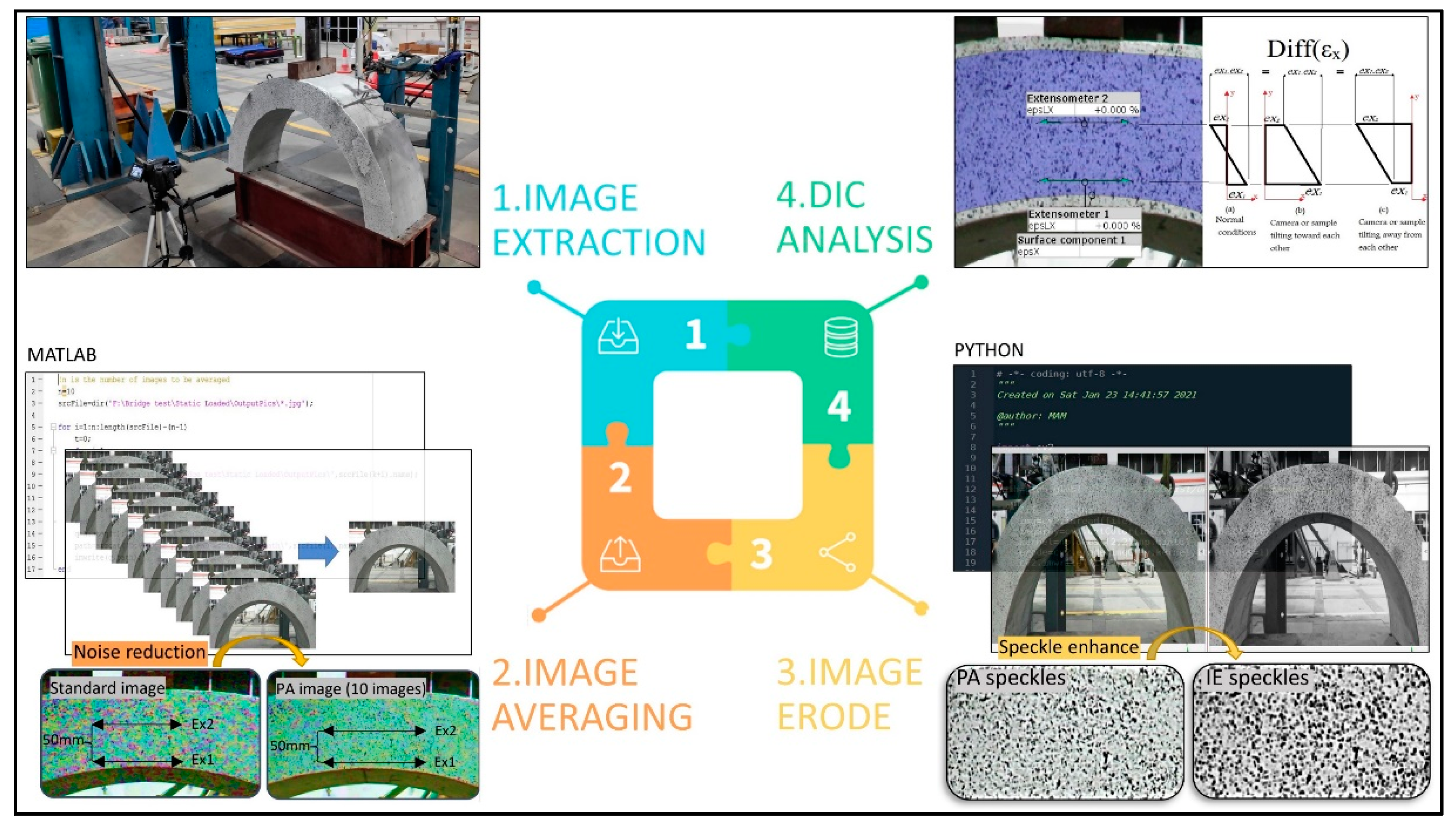
Two distinct image processing algorithms were used to reduce the deleterious effect from light noise and to process poor speckle applications. These techniques are (1) Pixels’ Averaging (P.A.) and (2) Image Eroding (I.E.). The methodology of this work is illustrated in
Figure 1. Three concrete arch bridges were tested under a single point of loading applied at the top middle part. The test was filmed using a DSLR camera for DIC analysis. Then, raw images are extracted and processed following the techniques illustrated in
Figure 1. Four imaging cases were investigated under similar DIC parameters, i.e., equivalent surface deformation components such as the subset size and distance, as presented in
Table 1. Also, a similar extensometer subset size and similar extensometer length were selected at the exact location in all cases for strain variations comparison. The extensometer locations were set at the middle part of the arch in the horizontal direction and 50 mm apart, as shown in
Figure 1. There are 12 cases divided into 9 cases regarding Pixel Averaging (P.A.) and the rest related to the Image Erode (I.E.) technique; refer to the last row of
Table 1. Each of the 9 (P.A.) cases computed the differential strain Diff (ε
x) between two horizontal extensometers in the middle of the arch and the linear least square criterion (R
2) between the two extensometers to establish the effect of image averaging on the strain variations. The last 3 cases are regarding the speckle pattern digital enhancement with the Image Erode (I.E.) technique. The (I.E.) cases were derived from the optimum cases of the (P.A.) approach. The cases are presented in
Table 1 and as follows:
1. Standard DIC images used for DIC analysis (S.I.). Only one image was extracted for every second of the test and used for strain variations analysis.
2. Pixels’ Averaged (P.A.) images, every image used for DIC analysis is generated by extracting and merging every ten frames of every second of the video. These (P.A.) images were developed by averaging every pixel in the image using a customized MATLAB code [
18].
3. Pixels’ Averaged (P.A.) images, every image is composed of 20 times the corresponding frames of every test’s second.
4. The optimum Pixels’ Averaged (P.A.) images are further processed with the Image Erode (I.E.) function developed by the OpenCV Python function used for speckle pattern enhancement (I.E.) [
19].
2.1. Pixel Averaging (P.A.)
The Pixel Averaging (P.A.) technique is a digital image processing method utilized to enhance videos and images damaged by random noise. In general, the pixel average or image averaging is utilized to remove the blurring of an image or video frame to provide smooth and sharp edges and reduce noise. The computational algorithm computes the arithmetic mean of the image’s grey intensity values of every corresponding pixel of the averaged frames. As a result, when the average of the image pixels is computed, the signal components will have a more decisive influence over the summation than the noise components. As shown in
Figure 1, the pixel averaged (P.A.) image noise (red-blue pixels) is less than the standard image. The mathematical formulation for this technique can be expressed in Equation (1):
where:
A: averaged intensity values of the image pixels,
N: number of averaged images (frames),
I: pixel intensity value of the
ith frame at the (
x,
y) location coordinates,
i: the frame index, and
x,
y: column and row coordinates of the image matrix, respectively.
It is worth noting that the (P.A.) technique is time independent such that merging of (n) number of images in this work does provide the same number of images used for standard DIC analysis as it initially extracts (n) counts the number of frames. However, it is essential to point out that using the (P.A.) technique is suitable for static loading applications such that the rate of strain change between the merged frames is negligible. Otherwise, in the case of high-strain rate applications, a ghosting effect is expected in the averaged images as motion is anticipated between the frames.
2.2. Image Eroding (I.E.)
Image Erode is one of the computer vision OpenCV python library kernels primarily used for microorganisms’ detection in biological images as well as utilized for interstellar object identification in astronomical images. As the name indicates, the Erode function works similarly to soil erosion to erode the boundaries of the foreground entities in digital images. The Erode kernel usually operates on binary and grayscale images requiring a dual input, the original image and the structuring kernel. The Erodes kernel usually works opposite its sister, the dilation kernel.
In the form of a grayscale erode, the kernel should have a height. The grayscale erosion of
H(
x,
y) by
I(
x,
y) is defined by Equation (2):
JI. is the domain of the kernel
I, and
H(
x,
y) is supposed to be +∞ outside the image domain.
x,
y: column and row coordinates of the image matrix, and
x′,
y′: column and row relative coordinates of the kernel [
20].
Mostly, the grayscale erode is applied with a flat Kernel (
I(
x,
y) = 0). The grayscale erosion is corresponding to a local-minimum operator shown by Equation (3):
The binary erode of
H(
x,
y) by
I(
x,
y), denoted
H ϴ
I, is identified as the set operation
H ⊖
I = {
k|(
Ik ⊆
H}. In other words, it is the set of locations
k, where the kernel moved to location k overlap only with the foreground pixels in
H [
20].
The Erode and the Dilation functions are illustrated in
Figure 2. As
Figure 2c shows, the Erode kernel shrinks the white color letter “
i” size shown in
Figure 2a in the black and white image as it calculates the local minimum over the kernel area. Then, the scanning Erode kernel replaces the image pixels under the overlapping kernel with a minimum pixel value. More information about this kernel can be found in the computer vision OpenCV documentation [
21]. In this work, the DIC requires high-contrast intensity images expressed in the field through randomly painted black speckle patterns over a white background. The image Erosion approach seems a perfect treatment for poorly painted surfaces and low-contrast images where it can be used to enhance, sharpen, and increase the size of the black speckles in the image domain.
3. Experimental Setup
The Digital Image correlation technique was utilized through an experimental campaign of three concrete arches tested by a Universal Tensile Machine (UTM) at the Heavy Structure & Strong Floor Laboratory, University of Sains Malaysia (USM). Three simply supported concrete arches were tested under a three-point bending loading to determine the arches working horizontal and vertical strains under the load. The load was applied manually using a hydraulic jack and 50 kN load cell at a monotonic rate of 1 kN increment. The arch surface was painted using white water-based paint, and then a black speckle pattern was realized through black paint sprayed over the white base. The test setup is illustrated in
Figure 3. The black speckles were sprayed inconsistently to simulate the condition of non-trained in-field applications. In addition, three Linear Variable Differential Transformer LVDTs were used to measure the arch deflection at the middle (one vertical LVDT) and the quarter (one horizontal and one vertical LVDT), as shown in
Figure 3. The Samsung DSLR camera has a 16 MP resolution with a video setting adjusted for indoor image acquisition. The camera was placed 80 cm from the arch surface, having a height similar to the arch. The camera was turned on 30 min before starting the test to avoid the errors produced by the camera heating [
22]. The video setting was set to 25 frames per second at 1080 P resolution. Three groups of images were extracted (1, 10, 20) frames per every second from every video captured for each specimen. The extracted images were uncompressed with a TIFF format.
Image averaging was implemented by taking every (10 or 20) frames and then merging (averaging) their pixels to a single image using a MATLAB code developed by the author. Next, the new optimized averaged pixel images were digitally eroded to increase the size of the speckle patterns. The eroding process was implemented to the (P.A.) images using the OpenCV-Python library, namely a (3 × 3) erode-dilation kernel. The Pixel Averaging (P.A.) and Image Erode’s (I.E.) pre-processing procedures are illustrated in
Figure 1.
A GOM correlates DIC software was used for the DIC analysis of the three cases; Standard Image (S.I.), Pixel Averaged (P.A.), and Image Erode (I.E.) images developed in this research [
23]. Similar DIC parameters were used for all three cases, a subset size (facet size) of 40 × 40 pixel and a subset distance (point distance) of 20 pixel for both surface and point components. Similar surface and point component locations were selected for all cases for results comparison. The differential strain between the two parallel horizontal extensometers of each sample (as shown in
Figure 3) was considered to avoid other 2D-DIC issues related to the sample or camera out-of-plane movement, as shown in
Figure 4.
4. Results and Discussion
The computed parameters were (1) the differential strain Diff(ε
x) (
Figure 4) between two horizontal extensometers in the middle of the arch and (2) the correlation between the two extensometers through finding the coefficient linear least square (R
2). The results of the maximum differential strain Diff(ε
x) against the number of averaged images, Diff(ε
x) range between the maximum and minimum Diff(ε
x) values, and the coefficient of least square (R
2) of the differential strain Diff(ε
x) are presented in
Table 2. The differential strain Diff(ε
x) values for each image case of the three tested arches are also respectively shown in
Figure 5,
Figure 6 and
Figure 7. The correlation between the two extensometer strain values from the DIC analysis of all image cases and arch samples is shown in
Figure 8,
Figure 9 and
Figure 10. The effect of image averaging on the initial guess of the correlation algorithm and strain variation is illustrated in
Figure 11. The Image Erode (I.E.) effect on the strain variation compared to the non-eroded Pixel Averaged images is shown in
Figure 5,
Figure 6 and
Figure 7. The (I.E.) effect on the speckle pattern density and surface component quality is shown in
Figure 12.
It is difficult to provide accurate and reliable strain values from the DIC analysis due to the high strain variation provided by the one-image cases, as shown in
Figure 5,
Figure 6 and
Figure 7 (the red series). Likewise,
Figure 5,
Figure 6 and
Figure 7 show that the 10 and 20 averaged image cases have lower differential strain variations than the one image cases of all arch samples. The differential strain Diff(ε
x) trend increases (tension bending) as the load grows with time. Therefore, the strain disparity of the one-image case can be attributed to the random light noise and not the actual material deformation.
Table 2 presents the maximum differential strain Diff(ε
x), which is defined as the last Diff(ε
x) value recorded during the test. It is shown from
Figure 5,
Figure 6 and
Figure 7 and
Table 2 that the maximum Diff(ε
x) for all samples approaches a specific strain range (~0.034) when the number of averaged images increases. It is reasonable to have comparable Diff(ε
x) values for the arch samples as they are made from the same concrete mix, cured under the same conditions, and tested under the same loading protocol. The Diff(ε
x) range is defined as the difference between the highest and lowest Diff(ε
x) of each image case of all samples. Equally, the range of maximum Diff(ε
x) reduces among all samples when averaged images are used for the DIC analysis. To clarify, when 20 averaged images are compared to the strain range (0.02–0.074) of the one image cases, all arch samples had maximum Diff(ε
x) values ranging between (0.034–0.035), as shown in
Table 2. In fact, the range of maximum Diff(ε
x) (0.054) of the one image cases is almost three times the Diff(ε
x) value (0.02) of the one image sample of arch B2, as shown in
Table 2.
Table 2 also shows that Diff(ε
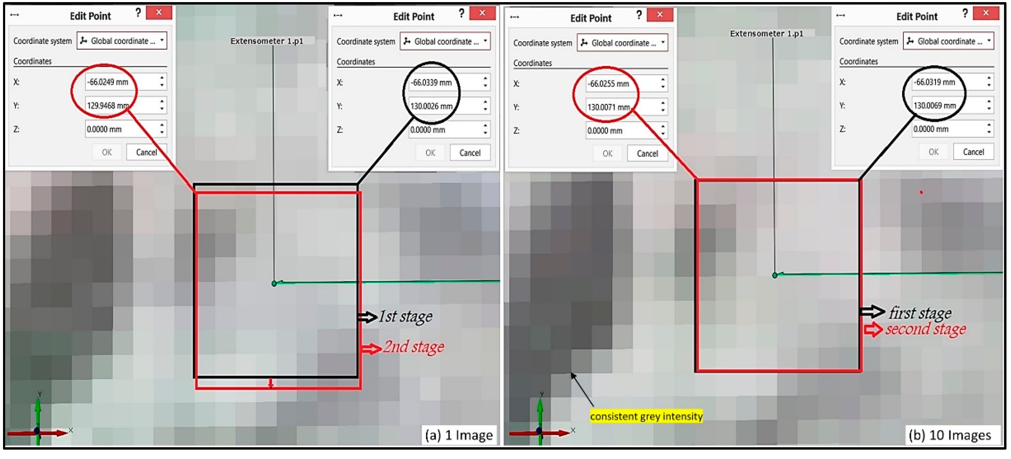
x) variance decreases up to 90% (in the case of sample B1) when the number of averaged images of each sample increases to 20. Overall, the strain variance decreases when the number of averaged images used for every stage of DIC analysis increases. The variance diminution is attributed to the extensometer subset’s initial guess (correlation peak) position being closer to the subset’s actual location for the averaged image than the single image. The clarification is presented in
Figure 11, which shows two consecutive stages of a single image and ten averaged images extensometer subsets. The close correlation peak estimation is credited to the high contrast and random noise reduction, providing speckles with more consistent grey intensities in the averaged images, as shown in
Figure 11.
The change of the coefficient (R
2) value (from 0.46 to 0.90, in the case of sample B3) implies a substantial improvement of the linear model representation when ten averaged images are utilized compared to the single image, as shown in
Table 2. However, only a marginal increase in the (R
2) values (from 0.90 to 0.92, in the case of sample B3) is observed between (10–20) images, as shown in
Table 2. Likewise, the growth of the (R
2) values of all arch samples when averaged images are used is reflected through the solid linear correlation trend between the two selected extensometers, as shown in
Figure 8b,
Figure 9b and
Figure 10b, compared to the scattering shown in
Figure 8a,
Figure 9a and
Figure 10a. However,
Figure 8c,
Figure 9c and
Figure 10c show an inappreciable enhancement of the linear correlation trend compared to
Figure 8b,
Figure 9b and
Figure 10b. The strong correlation in
Figure 8b,
Figure 9b and
Figure 10b and
Figure 8c,
Figure 9c and
Figure 10c provides further evidence of the minimization of strain variance.
It is worth noting that the strain values of each extensometer vary from one sample to another, as shown in
Figure 8,
Figure 9 and
Figure 10. The differences are produced by the lab testing circumstances, such as sample or camera movement. Therefore, selecting the differential strain Diff(ε
x) between the two extensometers should provide error-free of these influencing factors, as shown in
Figure 4. In summary, it is shown that the variance reduction and the improvement of (R
2) establish the positive impact of the Pixel Average (P.A.) technique on the accuracy of the acquired strain values. Thus, the 20 averaged images provide the most consistent Diff(ε
x) values and will be further used for the Image Erode (I.E.) cases.
The Image Erode (I.E.) approach requires grey images; therefore, the Pixel Average (P.A.) images are converted to grayscale images using the Open-CV(COLOR_BGR2GRAY) function. The Image Erode (I.E.) cases are derived from the 20 averaged images and processed with a (3 × 3) erode kernel for speckle enhancement. The (I.E.) samples of (B1 and B2) show a (26%) increase in the maximum differential strain Diff(ε
x) than their corresponding (P.A.) cases.
Figure 5 and
Figure 6 show that the (I.E.) Diff(ε
x) values are consistently higher than the (P.A.) Diff(ε
x) values which are attributed to the interpolation bias of the correlation subset. The correlation bias is initiated when the speckle size is expanded, making the initial guess tend to a specific region due to the high correlation provided by that region. The findings agree with the “image smoothing” approach suggested by Pan et al., 2013 to reduce the correlation bias error [
2].
Table 2 shows that the eroded images have a slightly higher variance (around 5%) than their corresponding 20 averaged images.
Table 2 shows a slight decrease in the (R
2) values due to the variance development. The variance increases in the (I.E.) images because of bias boosting of the subset due to speckle size enlargement. However, the quality of the surface pattern shows an enhancement compared to the (P.A.) images due to the weak correlation between the speckles, as shown in
Figure 12. The Image Erode’s (I.E.) primary objective is not to reduce the light variation but to enhance the contrast and increase the density of the poor speckle patterns. The Erode images provided more distinguishable speckle patterns, which helped to recognize microcracks and strain concentration regions in low-contrast images.
5. Conclusions
This work proposes two pre-processing methods to provide on-desk solutions for the Digital Image Correlation (DIC) random light noise problem. Two DIC’s significant challenges during the application, the high data variations and poor speckled surfaces, were treated using simple image processing techniques. The two approaches were developed using special computer software, Pixel Averaging (P.A.), developed with MATLAB code and Image Erode (I.E.) using OpenCV Python image processing package. The (P.A.) method was applied to the standard images captured while testing three simply supported concrete arches under a three-point bending flexural loading. Twelve cases were developed based on Standard Image (S.I.), Pixel Averaging (P.A.), and Image Erode (I.E.) to critically characterize and compare the maximum differential strain Diff(εx), Diff(εx) variance and its coefficient of linear least square (R2).
The Pixel Averaging (P.A.) technique provided consistent differential strain Diff(εx) values with a variance reduction of up to (90%) when averaged images were used for DIC analysis compared to the standard images. The coefficient of linear least square (R2) has also considerably increased from 0.46 to 0.90 (in the case of sample B3), which implies a substantial improvement of the linear model representation when ten averaged images are utilized compared to the single image. However, only a slight improvement of the (R2) value when twenty averaged images are used compared to the ten image cases.
The (I.E.) led to a slight increase in the Diff(εx) variance due to the correlation bias of the extensometers’ subset. The Image Erode (I.E.) approach provided qualitatively enhanced speckles with a highly consistent DIC surface component. The high surface component quality enables early crack detection by distinguishing the microcrack paths even when using low-contrast images.
The research highlights the importance of both approaches’ potential for DIC applications in the field where light conditions and test setups are challenging to control. The presented results encourage other image-enhancing approaches for more reliable data acquisition using the DIC technique. Finally, the image merging with the DIC technique can also be expanded to fields other than structural monitoring where the light and environmental conditions impede the use of the DIC technique.


