Article

Technical, Economic, and Environmental Trade-Offs in Pavements with Lime-Stabilized Soils: A Sustainability-Oriented Approach

by
Caroline Castilhos Rezende
,
Mônica Regina Garcez
*,
Thaís Radünz Kleinert
and
Washington Peres Núñez
Postgraduate Program in Civil Engineering: Civil Construction and Infrastructure, Federal University of Rio Grande do Sul, Porto Alegre 90035-190, Brazil
*
Author to whom correspondence should be addressed.
Infrastructures 2026, 11(9), 301; https://doi.org/10.3390/infrastructures11090301
Submission received: 21 May 2026 / Revised: 29 June 2026 / Accepted: 29 June 2026 / Published: 28 August 2026

Abstract

This paper proposes a sustainability-oriented approach to evaluate the incorporation of lime-stabilized soils into pavement systems as a strategy to reduce the environmental impacts associated with conventional unbound granular structures. Pavement sections were designed for three tropical subgrades (Argisol, Latosol, and Luvisol), considering five traffic levels ranging from low to high. Soil–lime layers containing 3% and 5% calcitic hydrated lime were compared with conventional unbound granular sections. Pavement design was performed through a mechanistic–empirical approach. Environmental impacts were quantified using life-cycle assessment from a cradle-to-construction perspective, including midpoint and endpoint indicators, and assessed together alongside relative construction costs. Pavement sections incorporating soil–lime layers reduced environmental impacts and relative costs for low and intermediate traffic levels, particularly for Argisol and Latosol subgrades. Reductions in global warming potential reached approximately 48%, while endpoint damage reductions exceeded 60% in some scenarios. However, the environmental benefits became progressively less pronounced as traffic levels increased. For the Luvisol subgrade, the lower suitability for lime stabilization required an additional graded crushed stone layer, reducing the environmental advantages of the stabilized systems. Soil–lime stabilization can represent an environmentally advantageous and economically competitive alternative for pavement design in tropical regions, particularly under low-to-moderate traffic conditions, although benefits may also be achieved at high traffic levels depending on subgrade characteristics.

1. Introduction

Increasing concerns about climate change and resource depletion have heightened the need to reduce the environmental impacts of road infrastructure [1]. In this context, adopting eco-efficiency principles in pavement design is essential to ensure that engineering solutions simultaneously meet performance requirements while minimizing environmental burdens.
The mechanical performance of asphalt pavements is strongly influenced by the stiffness and deformability of the supporting subgrade [2]. This aspect becomes particularly critical in tropical regions such as Brazil, where more than 80% of the territory is covered by tropical and subtropical soils [3]. Due to intense weathering and distinct mineralogical compositions, these soils exhibit engineering behavior that differs significantly from that in temperate regions, often exhibiting high compressibility, low strength, and pronounced volumetric instability [4]. To overcome these limitations, chemical stabilization techniques have been widely adopted, with lime among the most traditional and effective binders since the 1960s [5,6,7,8,9,10], using either quicklime (CaO) or hydrated lime (Ca(OH)2). The selection depends on soil characteristics, moisture conditions, material availability, and construction requirements. Both forms promote physicochemical reactions that improve the engineering properties of fine-grained soils, although hydrated lime is often preferred when ease of handling and uniform mixing are required [11]. Lime stabilization can significantly improve soil properties, including increased strength, enhanced resilient behavior, improved resistance to fatigue and permanent deformation, and reduced swelling potential [8,12,13,14,15,16,17,18,19]. Depending on soil characteristics, these improvements may allow lime-treated soils to be used not only as subgrade improvement but also as subbase or even base layers [20]. This enables reductions in asphalt layer thicknesses and the replacement of conventional granular materials with locally available soils, directly influencing construction costs and resource consumption.
Previous studies have investigated the environmental implications of incorporating lime into pavement systems, including its use as a soil stabilizer [21,22] and as a filler in asphalt mixtures [23]. From an environmental perspective, the use of locally available materials can significantly reduce impacts associated with raw material extraction and long-distance transportation [21], particularly in regions where high-quality aggregates are scarce and logistics costs are high [24]. However, the environmental performance of lime-stabilized systems is not straightforward. While reductions in material transport and aggregate use may lower environmental burdens, lime production itself is highly energy-intensive, with calcination processes contributing significantly to greenhouse gas (GHG) emissions [24,25,26,27]. In some cases, more than 75% of impacts related to energy consumption, GHG emissions, and photochemical oxidation have been attributed to lime production. Furthermore, previous studies have shown that asphalt layers account for the majority of CO2 emissions in pavement systems due to energy-intensive production processes [28,29], highlighting the complexity of environmental trade-offs in pavement design.
Despite the recognized mechanical and economic advantages of lime-stabilized systems [8,19,30,31,32,33,34,35,36] and the growing body of research on pavement sustainability and soil stabilization techniques [5], comprehensive studies quantifying their environmental performance under realistic design conditions are still limited [21,22,27,37]. In particular, there is a gap in studies that adopt a cradle-to-construction approach, accounting for the interactions among structural design parameters, material availability, and transportation logistics. Furthermore, the overall sustainability of lime-treated pavements depends on multiple factors, including soil type and lime content, which influence mechanical performance and structural design requirements of the pavement, as well as traffic levels, material availability, and transportation distances, which are key parameters affecting environmental impacts [21,25,26,27]. The recent literature often relies on simplified assumptions, limited system boundaries, or generic life-cycle inventory (LCI) data that do not adequately reflect regional conditions [38,39,40,41]. Moreover, inconsistent modeling approaches reduce transparency and hinder reproducibility and comparability across studies. As a result, there is still no clear understanding of the conditions under which lime stabilization provides net environmental benefits when applied to pavements, particularly in tropical regions. As a consequence, the environmental trade-offs between reduced material transport and the high impact of lime production are not fully understood, and there is still no context-sensitive framework to support decision-making regarding the use of lime stabilization in pavements.
Thus, this paper aims to bridge the gap between geotechnical performance, economic, and environmental trade-offs by developing a framework to support more sustainable decision-making in the design of pavements incorporating lime-stabilized soils. The analysis integrates pavement design, cost evaluation, and an LCA within a cradle-to-construction perspective, considering three tropical soils (Argisol, Latosol, and Luvisol), two lime proportions (3% and 5%), and traffic levels ranging from low to high. The main objective is to identify the conditions under which lime stabilization represents a sustainable alternative to conventional granular solutions. In addition, this study contributes to improving transparency and reproducibility in LCA applications for pavement engineering.

2. Method

The sustainability-oriented approach proposed in this paper (Figure 1) integrates pavement design, cost, and environmental impact data to identify the conditions under which lime stabilization represents a sustainable alternative to conventional unbound granular solutions.

2.1. Pavement Design

The pavement design followed the South African mechanistic–empirical design guidelines [42], which provide field-calibrated predictive models for pavement distress mechanisms associated with granular base shear failure, permanent subgrade deformation, fatigue and crushing of cemented layers, and fatigue cracking of asphalt layers.
The soils (Argisol, Latosol, and Luvisol from Brazil) were used as subgrade materials for the pavements in their natural condition. For each subgrade type, two pavement configurations were defined: (i) unbound granular, consisting of granular base and subbase layers, and (ii) soil–lime, in which soil–lime mixtures were used in association with the corresponding subgrade soil.
Traffic volume was adopted as the equivalency factor for the design of the different pavements to ensure that all alternatives had the same service life. Five traffic scenarios were defined (N1 = 1.00 × 10⁶, N2 = 5.00 × 10⁶, N3 = 1.00 × 10⁷, N4 = 5.00 × 10⁷, N5 = 1.00 × 10⁸) based on cumulative equivalent standard axle loads (ESALs), following the traffic ranges suggested by the Brazilian National Department of Transport Infrastructure (DNIT) [43]. These traffic levels were selected as representative design scenarios spanning low to very high traffic conditions to evaluate the influence of traffic demand on pavement design, life-cycle costs, and environmental impacts. The loading condition consisted of a single axle with dual wheels and a load of 8.2 tf under a tire pressure of 560 kPa [43].
For each trial pavement section, the multilayer elastic analysis routine (AEMC, version 2.4.2) available in Brazilian Pavement Design Method–MeDiNa software [44] was used to determine, through non-linear analysis, the stresses and strains at critical locations within the pavement structure. The analysis points were defined at the midpoint between the dual wheels and below the center of one wheel. The evaluated depths included the bottom of the asphalt surface layer, the midpoint of the granular layers (base and subbase), and the top of the subgrade. For pavements with soil–lime layers, the top and bottom of the stabilized layer were also considered points of interest.
The calculated structural responses were then used as inputs to the corresponding prediction models in the South African mechanistic–empirical design guidelines [42] to estimate the allowable number of ESALs for each distress mechanism, with a reliability level of 90%. The pavement layer thicknesses were adjusted iteratively until all distress criteria satisfied the target design traffic level. The governing design criterion corresponded to the distress mechanism associated with the lowest allowable ESALs, and was reported as the controlling failure mode for each pavement structure: fatigue cracking of the asphalt layer, shear failure of the granular layer, permanent deformation at the top of the subgrade, and fatigue and crushing of the cemented layer. Due to the lack of experimental data regarding the post-cracking and post-crushing behavior of lightly cemented layers and to adopt a conservative approach, residual service lives were not computed.

2.2. Materials

2.2.1. Subgrade

Three soil types were investigated following the Brazilian Soil Classification System [45]: red-yellow Argisol, red Latosol, and haplic Luvisol. Argisols and Latosols cover approximately 24% and 39% of Brazil’s surface area, respectively, whereas Luvisols account for a smaller proportion, corresponding to about 3% of the national territory [46]. The soils were selected based on both pedological representativeness and practical relevance for pavement engineering. Argisol and Latosol are among the most widespread tropical soil classes in Brazil and are frequently encountered in road infrastructure projects. Luvisol represents a soil with distinct geotechnical characteristics and a different response to lime treatment, enabling the evaluation of lime-induced improvements across a wider range of soil conditions. For all three sampling locations considered in this study, lime treatment is a potential strategy for improving local materials for pavement construction. This approach enabled the environmental and structural performance of soil–lime systems to be assessed across soils with varying responsiveness to stabilization.
Table 1 and Table 2 present the properties of Argisol, Latosol, and Luvisol, along with the coefficients and statistical significance of the composite models developed by Kleinert [47] for resilient modulus prediction based on repeated-load triaxial testing, respectively.
The AASHTO A-7-5 classification designates a fine-grained clayey–silty soil with poor performance as a highway subgrade material. According to the USCS, ML (Argisol) corresponds to an inorganic silt with low to medium plasticity, whereas MH (Latosol and Luvisol) represents a high-plasticity elastic silt that may be susceptible to significant volumetric changes. It is important to note that both the AASHTO and USCS classification systems were originally developed for soils from temperate regions. Consequently, they do not fully capture the distinctive engineering behavior of residual soils formed under tropical and subtropical climatic conditions. The Brazilian MCT classification provides a more representative characterization of the behavior of the tropical soils investigated in this study. While the AASHTO and USCS classification systems generally classify fine-grained soils as poor pavement subgrades, the Brazilian MCT classification recognizes that the performance of tropical soils depends not solely on grain-size distribution or plasticity and consequently some clayey tropical soils may exhibit satisfactory mechanical performance and perform well as pavement subgrades. According to the MCT system, Argisol is classified as NS’ (non-lateritic silty soil), Latosol as LG’ (lateritic clayey soil), and Luvisol as NG’ (non-lateritic clayey soil). Lime treatment promotes different improvements depending on soil type, reducing instability and water sensitivity in non-lateritic soils (NS’ and NG’) and increasing stiffness and structural strength of lateritic soils (LG’) [4].
From the chemical perspective, the phosphorus content in the Argisol and Latosol is very low, whereas the Luvisol exhibited a medium phosphorus content [55]. Regarding potassium, its concentration was classified as low in the Argisol, medium in the Latosol, and very high in the Luvisol [55]. The Luvisol presented a high CEC, reinforcing its expansive behavior. The Argisol exhibited the lowest CEC value. The CEC observed for the Latosol is characteristic of highly weathered clay-rich soils lacking expansive clay minerals. All three soils contained organic matter; however, only the Luvisol exhibited organic matter content exceeding 1%. The Argisol showed the lowest base saturation and the highest exchangeable aluminum content, whereas the opposite trend was observed for the Luvisol. In a study involving tropical soils, Rezende [56] reported that higher levels of exchangeable aluminum are associated with a greater potential for improvement through lime stabilization.
All three soils contained more than 25% material passing a no. 200 sieve (0.075 mm) and exhibited plasticity indices greater than 10%, meeting the criteria suggested by the National Lime Association [13] for lime stabilization.

2.2.2. Soil–Lime Mixtures

Table 3 presents the physical and mechanical properties of the soil–lime mixtures developed by Kleinert [47] with 3% and 5% calcitic hydrated lime as input parameters for the pavement design. Lime contents of 3% and 5% represent a range of practical stabilization dosages commonly adopted for tropical fine-grained soils, allowing assessment of both minimum effective treatment and enhanced stabilization conditions. The mix design followed the pH procedure [57], which was performed on soil passing the 40 sieve (425 μm) to determine the minimum lime content required to achieve a soil–lime mixture pH of 12.4, ensuring sufficient alkalinity to sustain the pozzolanic reactions necessary for soil stabilization. The strength results for the lime-treated mixtures indicated that the Argisol was suitable for lime stabilization under both standard and modified compactive efforts, with mixtures compacted using the modified effort exhibiting higher strength values. For the Latosol, lime stabilization required a modified compactive effort. The Luvisol did not demonstrate adequate lime stabilization performance, and was therefore classified only as a lime-improved soil rather than a stabilized material. Consequently, standard compactive effort was adopted for the Luvisol mixtures.

2.2.3. Granular Layers

The granular layers consist of graded crushed stone used as the base course and macadam classified as G4 material according to the South African pavement classification system [46] used as the subbase course (Table 4).

2.2.4. Bituminous Interlayer Treatments

The prime coating material applied between the granular base layer and the asphalt surfacing to improve resistance to water infiltration consists of CM-30 cut-back asphalt (0.001 t/m2) [66,67]. The tack coat applied to ensure adhesion between asphalt pavement layers consisted of a RR-1C rapid-cure cationic emulsion (0.001 t/m2) [68].

2.2.5. Surface Layer

The wearing course consisted of hot-mix asphalt (HMA). For pavement design purposes, the asphalt concrete mixtures followed DNIT Range B with a resilient modulus of 3000 MPa, and DNIT Range C with a resilient modulus of 8000 MPa gradations (Table 5) with Pen 50/70 binder. A Poisson’s ratio of 0.30 and a specific gravity of 23.5 kN/m3 were considered. The values adopted for the asphalt mixtures correspond to standard assumptions recommended by the MeDiNa [44] and are commonly used as reference values in mechanistic pavement analyses. The mentioned values were applied to all pavement sections, allowing the influence of base layer materials to be assessed without introducing additional variability associated with asphalt mixture properties.

2.3. Life-Cycle Assessment

2.3.1. Goal and Scope Definition

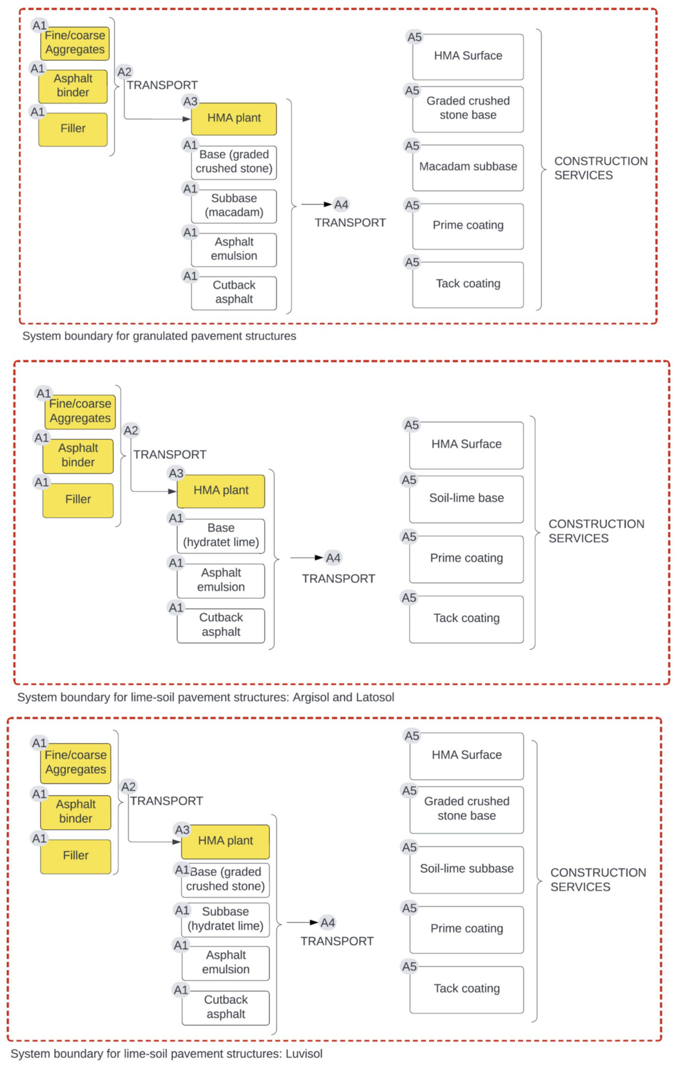
The sustainability-oriented framework proposed in this study includes an LCA following the ISO 14040 [70] and 14044 [71] standards aimed at identifying the conditions under which lime stabilization constitutes a more sustainable alternative to conventional granular solutions in terms of environmental impacts, thereby enabling subsequent comparison with economic performance. The LCA adopts a cradle-to-construction (A1 to A5 stages of the system boundary) approach to focus on the environmental impacts associated with product (A1 to A3), transport (A4), and construction (A5) stages of ISO 21931-2 [72], as illustrated in Figure 2. This approach is appropriate for isolating the effects of material selection and logistics on pavement life-cycle impacts. The functional unit corresponds to 1 km of pavement consisting of two 3.5 m-wide traffic lanes, including the subbase, base, and surface layers. The use phase was not within the scope of the present LCA, as all pavement alternatives for a given traffic level were designed to achieve the same service life.

2.3.2. Inventory Analysis

The inventory comprises foreground data related to the production and construction stages and background data from the Ecoinvent database version 3.12 [73] for Open LCA software [74] using regional providers (BR) as much as possible or RoW/GLO for unavailable national data. The foreground for materials depends on the configuration of each pavement section, whereas transport distances vary according to the location of each subgrade soil and nearest material suppliers, and energy consumption was estimated using the Brazilian Cost Reference System [69].
The inventory for the product stage (A1 to A3) accounts for the following materials: coarse aggregate for the base and subbase, cut-back asphalt and asphalt emulsion for interlayer treatments, and HMA for the surface layer, as detailed in Table 6.
In Table 6, material quantities depended on the configuration of each pavement section presented in Section 3. For aggregates, filler, hydrated lime, and bitumen, the quantities are based on the pavement layer dimensions, material densities, and mixture compositions presented in Section 2. For interlayer treatments, material consumption was estimated using the respective application rates per unit area (m2) reported in Section 2. Transport distances for the A2 stage were defined based on the specificities of each subgrade soil (Table 7) using the suppliers closest to the locations where the soils occur and where the corresponding paving works could potentially be implemented.
The inventory for the construction stage (A4–A5) accounts for the transport of materials to the site (A4) and the energy for pavement construction (A5).
The transport stage (A4) accounts for the transport of coarse aggregate, hydrated lime, cut-back asphalt, asphalt emulsion, and HMA to the field, as described in Table 8. The transport distances were defined based on the specificities of each subgrade soil (Table 7), using the suppliers closest to the locations where the soils occur and where the corresponding paving works could potentially be implemented.
The energy consumed during the construction stage (A5) was estimated using the Brazilian Cost Reference System [69], considering materials, equipment, and productivity (Table 9). A specific set of equipment was considered for each service type (Table 10), taking into account crew and equipment productivity, fuel consumption, and the power of each piece of equipment. The total number of hours required for each service was determined by dividing the total service quantity by the crew productivity per hour. Subsequently, the consumption of each piece of equipment was calculated based on its power and the operational productivity associated with each service. The consumed energy was the sum of diesel consumption converted to kWh and equipment electricity consumption, in kWh.

2.3.3. Impact Assessment

The life-cycle impact assessment was performed using the CML (baseline) method developed by Leiden University [75], considering the following midpoint impact categories: ozone depletion (kg CFC-11 eq); abiotic depletion (fossil fuels) (MJ); abiotic depletion (elements) (kg Sb eq); global warming potential (GWP, 100-year) (kg CO2 eq); photochemical oxidation (kg C2H4 eq); acidification (kg SO2 eq); freshwater aquatic ecotoxicity (kg 1,4-DB eq); marine aquatic ecotoxicity (kg 1,4-DB eq); terrestrial ecotoxicity (kg 1,4-DB eq); eutrophication (kg PO43− eq); and human toxicity (kg 1,4-DB eq). A complementary analysis was conducted by grouping the normalized midpoint results into three areas of protection (ecosystem quality, human health, and resources) using the CML-IA normalization factors. This approach provided an integrated perspective on the relative contribution of the different environmental impact categories while supporting the conclusions derived from the midpoint assessment.

2.4. Costs

Construction and transport costs were estimated based on Brazilian National Department of Transport Infrastructure guidelines [76,77], the service composition data obtained from the Brazilian Cost Reference System [69], and the database of the Brazilian National Agency of Petroleum, Natural Gas and Biofuels [78]. The total cost comprises the unit cost of each service composition calculated as the sum of the unit cost corresponding to the service execution, RIF cost (rain influence factor), TIF cost (traffic influence factor), total material unit cost, and total fixed time unit cost (cost of loading and unloading in the transport of materials) [29].

3. Results and Discussion

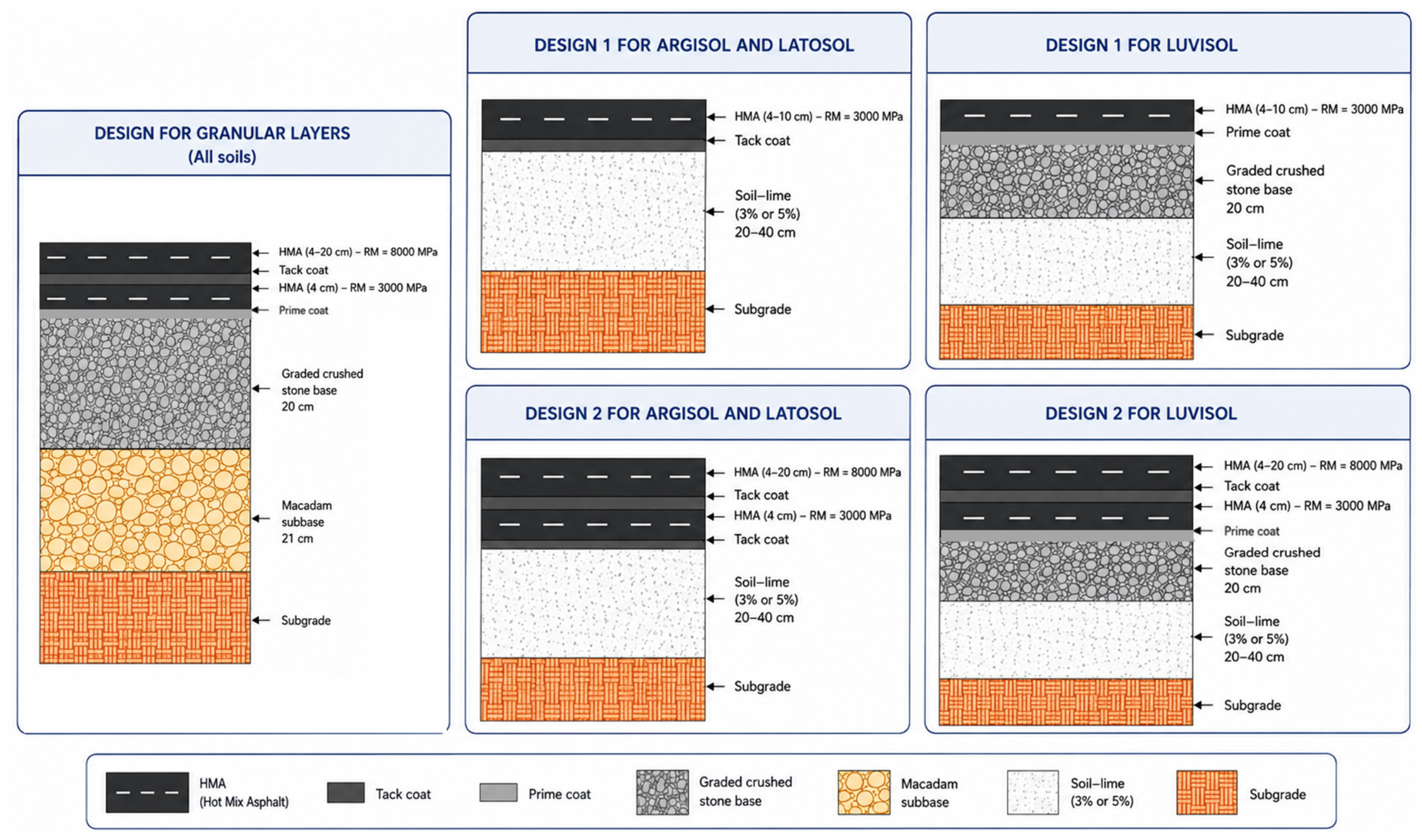
Figure 3 illustrates the pavement sections detailed in Table 11, Table 12, Table 13 and Table 14. For the Argisol and Latosol subgrades, the pavements consisted of a lime-stabilized layer combined with an asphalt surface layer. For the Luvisol subgrade, an additional graded crushed stone base layer was introduced between the lime-improved system and the asphalt surface layer to compensate for the lower suitability for lime stabilization [4].
Granular pavement structures were designed with a fixed base thickness of 20 cm and a subbase thickness of 21 cm. For the soil–lime alternatives, the stabilized layer thickness ranged from 20 to 40 cm for Argisol and Latosol subgrades. For the Luvisol subgrade, a lime-improved layer ranging from 20 to 40 cm was combined with a 20 cm graded crushed stone base layer.
Regarding the asphalt surfacing, two design approaches were considered, as illustrated in Figure 3. In Design 1, a single asphalt mixture with a resilient modulus of 3000 MPa was used throughout the entire asphalt layer. In Design 2, two asphalt mixtures were adopted: a lower asphalt layer with a resilient modulus of 3000 MPa and an upper asphalt layer with a resilient modulus of 8000 MPa. For Design 2, the thickness of the lower asphalt layer was fixed at 4 cm, while the remaining asphalt thickness required by the pavement design was assigned to the upper layer. To ensure adequate compaction and construction quality, a maximum thickness of 7 cm was adopted for both design options, consistent with common Brazilian pavement construction practices [79]. Consequently, the asphalt layers were subdivided into multiple layers whenever necessary. This distinction is particularly relevant, because the number of asphalt layers directly affects the quantity of tack coat required. Since tack coat applications were included in both the cost and life-cycle assessment inventories, the adopted asphalt layer configuration influences the economic and environmental performance of the pavement sections.
Regarding interlayer treatments, tack coats were applied between successive asphalt layers and at the interface between asphalt and soil–lime layers to ensure adequate adhesion between adjacent bound layers. A prime coat was considered at the interface between a graded crushed stone layer and an overlying asphalt layer. Consequently, all pavement sections with a graded crushed stone base layer required a prime coat. The same assumption was adopted for the Luvisol pavement sections, in which a graded crushed stone base layer was included above the lime-improved layer.
A remarkable difference between pavements incorporating unbound granular and soil–lime layers is due to the HMA thickness. Pavements containing soil–lime layers required thinner asphalt courses than conventional unbound granular structures under the same traffic conditions (Table 11, Table 12, Table 13 and Table 14). This behavior is associated with the enhanced load-bearing capacity and compressive strength provided by lime stabilization [4,47]. Lime addition increases the soil cohesion and stiffness, enabling the stabilized layer to withstand traffic loads more efficiently and consequently reducing the required HMA thickness compared with conventional unbound granular bases [47].
For the Argisol subgrade, lime stabilization resulted in a substantial increase in structural capacity, enabling the greatest reduction in HMA layer thickness under the same traffic level. The HMA thickness reduced from 9.5–19.5 cm (granular layer) to 4–12 cm (3% soil–lime layer) and 4–11 cm (5% soil–lime layer). The HMA thickness for the Latosol subgrade reduced from 9–20 cm (granular layer) to 4–19 cm (3% lime-sol layer) and 4–14 cm (5% soil–lime layer). Although the beneficial effects of lime improvement were still observed in the Luvisol subgrade, they were less pronounced than in the Argisol and Latosol.
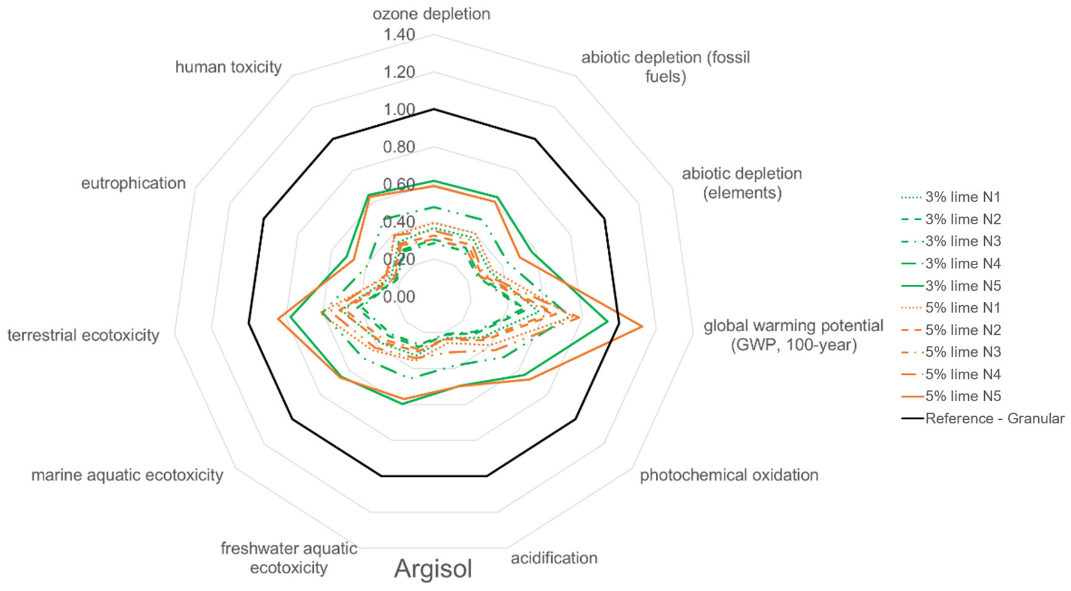
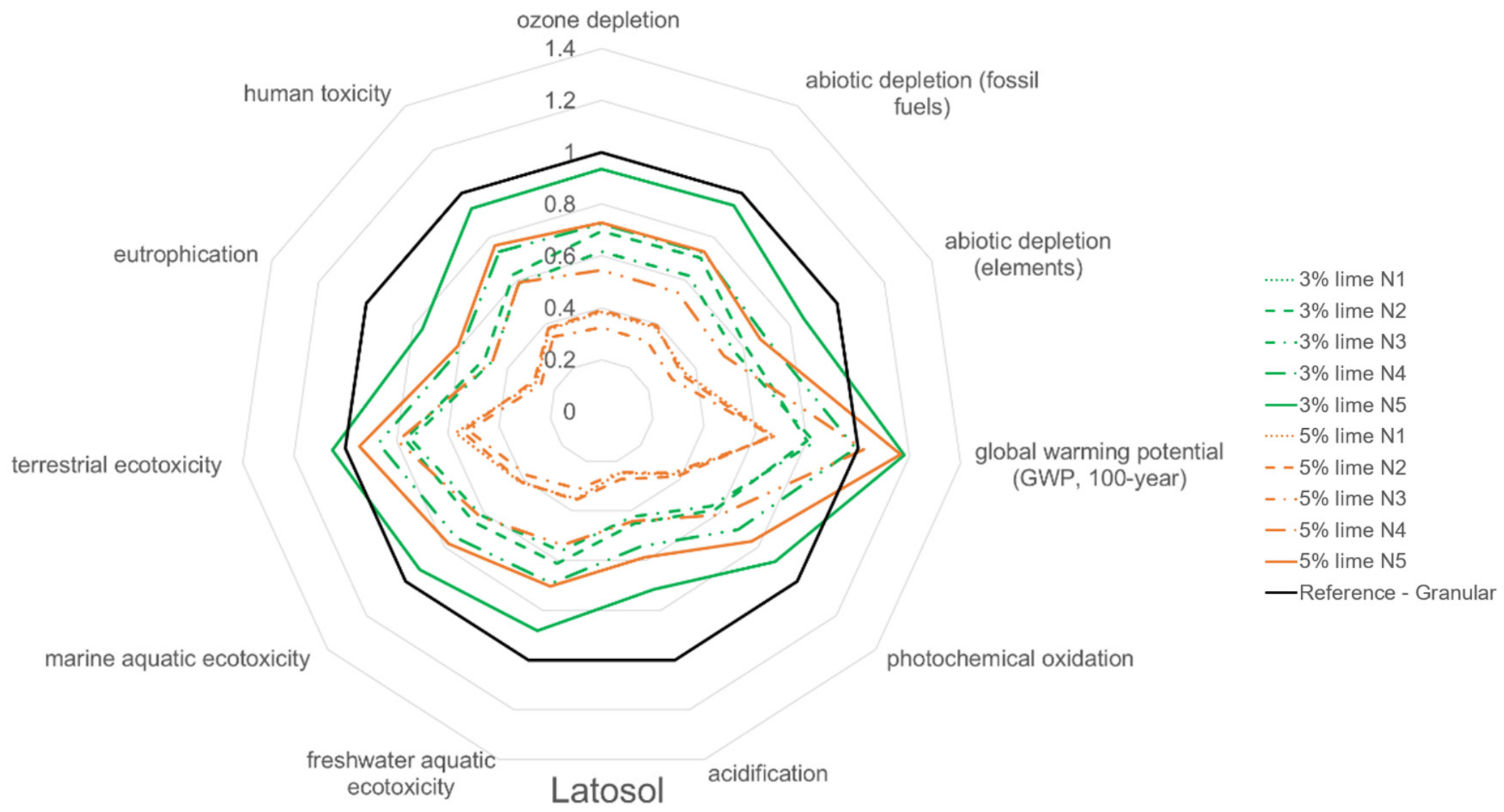
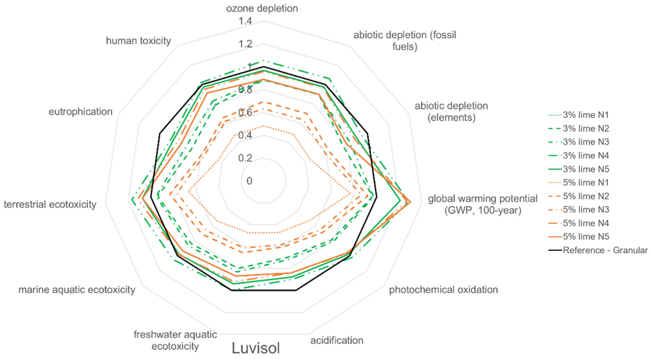
Figure 4, Figure 5 and Figure 6 provide a visual comparison of the environmental impacts of pavement sections incorporating soil–lime layers relative to the corresponding reference sections composed of unbound granular materials at each traffic level, highlighting overall trends and differences among the alternatives, whereas Table 15, Table 16 and Table 17 present the corresponding numerical values to support detailed quantitative analysis. In Table 15, Table 16 and Table 17, environmental impact ratios below 1.00 are highlighted in green, indicating that the soil–lime pavement sections exhibited lower impacts than their corresponding granular reference sections. Ratios between 1.00 and 1.20 are highlighted in yellow, indicating marginal increases in impacts, while ratios greater than 1.20 are highlighted in red, indicating increases exceeding 20% relative to the reference sections.
The results show that regardless of the subgrade soil, pavement sections incorporating soil–lime layers generally result in reduced environmental impacts compared to their respective references. In general, the reduction in environmental impacts becomes less pronounced as traffic levels increase from N1 to N5. The reduction in environmental impacts is more pronounced for the Argisol subgrade, followed by the Latosol and Luvisol.
For Argisol, soil stabilization with 3% and 5% lime resulted in similar reductions in environmental impact. Less favorable results were observed for the highest traffic level (N5), for which soil stabilization with 5% lime did not reduce emissions associated with global warming potential. Pavements stabilized with 5% lime exhibited global warming potential ratios of 0.75, 0.66, and 0.63 for traffic levels N1 to N3, respectively, indicating reductions of 25%, 34%, and 37% compared with the corresponding granular pavement sections. As traffic demand increased, the relative advantages decreased, and the global warming potential increased 12% for N5. Similar trends were observed for the remaining impact categories, though with substantial reductions.
Regarding the Latosol, soil stabilization with 5% lime provided greater reductions in environmental impacts than stabilization with 3% lime across all traffic levels. However, slightly higher CO2-eq emissions were observed for both 3% (1.18) and 5% (1.17) lime stabilization at the highest traffic level (N5), while the section stabilized with 5% lime showed CO2-eq emissions comparable to the reference at traffic level N4 (1.02).
The environmental benefits were less pronounced for the Luvisol subgrade, particularly with respect to global warming potential at higher traffic levels (N4 and N5), where results exceeded those of the respective reference sections by 20–30%, regardless of lime content. This behavior is associated with the lower effectiveness of lime treatment for Luvisol, which requires thicker pavement sections. Nevertheless, environmental benefits were still observed for several other impact categories, especially for traffic levels N1 to N3.
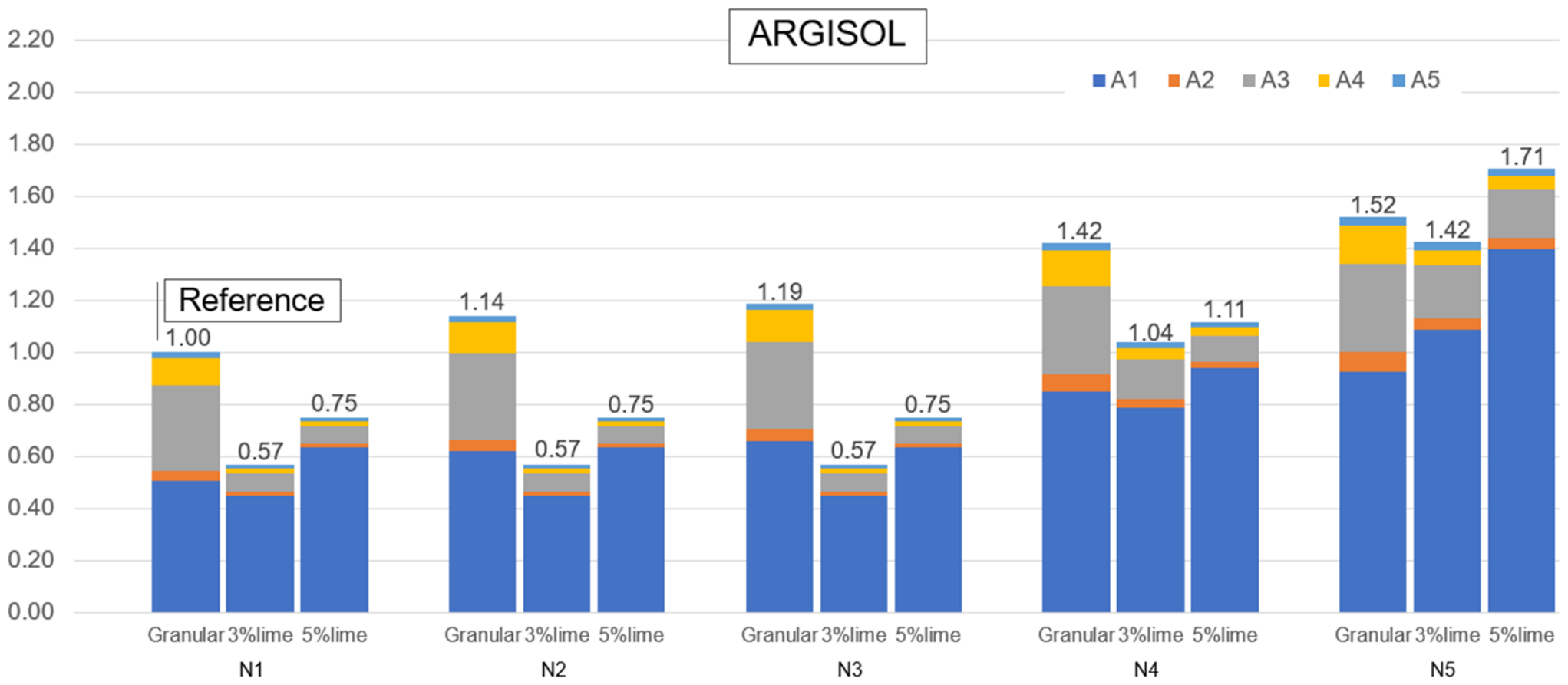
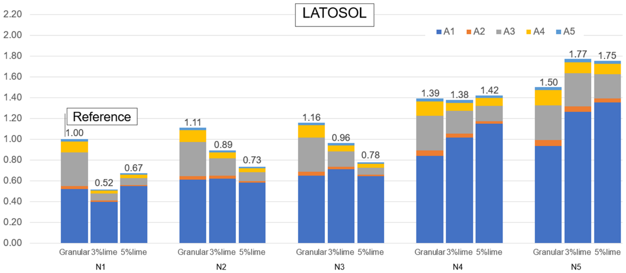
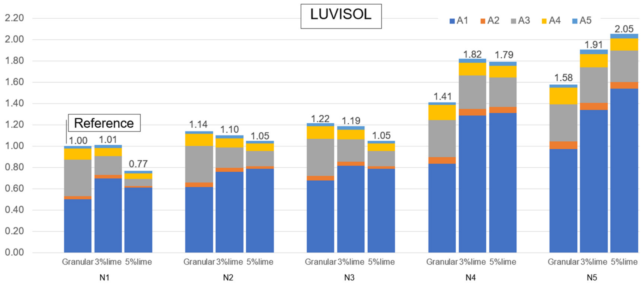
Figure 7, Figure 8 and Figure 9 show the global warming potential of the pavement sections incorporating soil–lime layers relative to the reference section composed of unbound granular material designed for low traffic (N1). The results disaggregated by life-cycle stage highlight the relative contributions of the material production (A1 to A3), transportation (A4), and construction (A5) stages to the overall impacts.
The A1 stage, corresponding to material production, accounts for the largest share of the global warming potential indicator, followed by the A3 stage, associated with HMA production, and the A4 stage, related to transporting materials to the construction site.
Hydrated lime (953 kg CO2-eq/t) and the asphalt binder (828 kg CO2-eq/t) used to produce the HMA are the primary contributors to global warming potential in the A1 stage. Although the pavement sections incorporating soil–lime layers exhibited lower emissions from the HMA surface layer, these reductions were partially offset by additional emissions from hydrated lime addition. As an example, in the case of Argisol subgrade, soil stabilization with 5% lime, and traffic level N5, the reference scenario (unbounded granular layer) demands 3272 t of HMA (202 t of asphalt binder), whereas the 5% lime scenario accounts for 1848 t of HMA mixture (112 t of asphalt binder plus 247 t of hydrated lime for soil stabilization. As a result, emissions in the A1 stage are higher for the soil–lime section.
The reductions in global warming potential in the A3 and A4 stages are the main contributors to reducing emissions in pavement sections designed with soil–lime layers. Indeed, the reduction in HMA layer thickness leads to a significant decrease in impacts associated with the A3 stage, since in the built inventory, the HMA production releases 25.5 kg CO2-eq/t of asphalt mixture (72.88 kWh/t).
In general, pavement sections incorporating soil–lime layers showed a notable reduction in emissions associated with the transportation of materials (0.134 CO2-eq/tkm) to the construction site (A4 stage). A more pronounced reduction was observed in the Argisol subgrade, regardless of traffic level, followed by the Latosol subgrade. For the Luvisol subgrade, the reduction in A4 stage-related emissions was less pronounced because an additional 20 cm of graded crushed stone base layer was required to compensate for the soil’s lower suitability for lime stabilization, thereby increasing transportation-related emissions during the A4 stage.
The global warming potential increased with traffic level across all pavement sections and subgrade conditions, reflecting the progressive increase in pavement thickness required to withstand higher traffic demands. For the Argisol and Latosol subgrades, pavement sections incorporating soil–lime layers exhibited lower global warming potential than the reference unbound granular sections, especially at low and intermediate traffic levels (N1 to N3). As traffic levels increased, the benefits in terms of global warming potential decreased. A similar trend was observed for the Luvisol subgrade, although the increase in global warming potential emissions with traffic level was more pronounced. For N4 and N5, the pavement sections containing soil–lime layers exhibited global warming potential values comparable to or higher than those of the unbound granular sections.
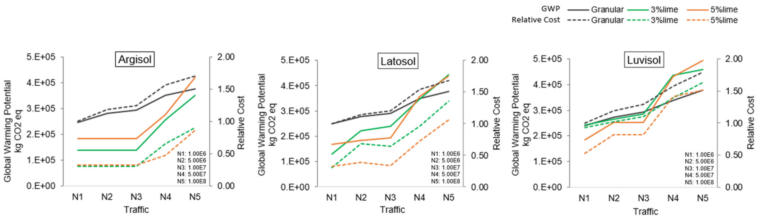
Figure 10 illustrates the relationships between relative cost and global warming potential emissions for pavement sections with unbound granular and soil–lime layers for different traffic levels and subgrade soils.
For the Argisol and Latosol subgrades, pavement sections incorporating soil–lime layers exhibited lower relative costs and CO2-eq emissions than the reference granular sections at low and intermediate traffic levels (N1 to N3). In these cases, using 3% lime generally resulted in lower CO2-eq emissions and costs than using 5% lime, indicating that increasing lime content does not necessarily improve global warming potential or economic performance. However, from traffic level N4 onward, both costs and CO2-eq emissions increased substantially for the soil–lime alternatives, approaching or even exceeding the values observed for the unbound granular reference sections, particularly for the mixtures containing 5% lime. For the Luvisol subgrade, the environmental and economic benefits associated with soil–lime stabilization were less pronounced. Although the stabilized sections remained competitive on cost at lower traffic levels, global warming potential emissions increased significantly for N4 and N5, especially with the 5% lime improvement, whose emissions surpassed those of the unbound granular section. The results indicate that the use of soil–lime layers is particularly advantageous for low-to-moderate traffic conditions, especially for Argisol and Latosol subgrades. For high traffic levels and less reactive soils such as Luvisol, the benefits become progressively less evident.
Table 18, Table 19 and Table 20 show the life-cycle impacts for the functional unit, normalized by dividing each midpoint impact result by the corresponding normalization factors of the CML-IA method, and grouped into three damage categories: ecosystem quality, human health, and resources. Ecosystem quality represents the potential damage to ecosystems, biodiversity, and ecological functions caused by emissions and resource use, while human quantifies the potential effects of environmental burdens on human well-being and mortality/morbidity, and the resources category evaluates the depletion of natural resources. The results are presented for the pavements designed for intermediate traffic (N3) with unbound granular and soil–lime layers treated with 5% lime. N3 was the highest traffic level at which none of the midpoint impact categories exceeded the impacts of the corresponding reference pavement sections, while the 5% lime content showed favorable environmental benefits, particularly regarding global warming potential.
The normalized life-cycle impacts for the functional unit indicate that pavement sections incorporating soil–lime layers (5% lime, traffic level N3) reduced impacts across all areas of protection. For ecosystem quality, the reductions reached 65% for the Argisol subgrade, 63% for the Latosol subgrade, and 34% for the Luvisol subgrade. Similar trends were observed for the human health category, with reductions of 65%, 63%, and 36% for the Argisol, Latosol, and Luvisol subgrades, respectively. In the resource damage category, the reductions reached 68% for both the Argisol and Latosol subgrades and 36% for the Luvisol subgrade.
The results presented in this paper demonstrate that soil–lime stabilization can serve as a viable pathway toward lower-impact, more sustainable pavement infrastructure systems.

4. Conclusions

This paper proposes a sustainability-oriented approach to evaluate trade-offs in pavements with lime-stabilized soils from a cradle-to-construction perspective. The paper demonstrates that the sustainability performance of soil–lime pavements depends on the specificities of subgrade soils and traffic conditions. The following conclusions can be drawn.
  • For Argisol and Latosol subgrades, pavement sections incorporating soil–lime layers generally exhibited lower environmental impacts than the corresponding unbound granular sections, particularly under low and intermediate traffic levels.
  • The environmental benefits of soil–lime stabilization decreased as traffic demand increased, mainly because thicker asphalt layers were required to meet structural design criteria.
  • The environmental and economic performance of soil–lime pavements was highly dependent on subgrade characteristics. While Argisol and Latosol showed substantial benefits from lime treatment, the advantages were less pronounced for Luvisol, particularly under high traffic levels.
  • Despite the increase in emissions associated with hydrated lime production during the A1 stage, pavement sections with soil–lime layers often achieved lower overall impacts in the cradle-to-construction perspective due to reductions in HMA thickness and lower transportation-related emissions during the A3 and A4 stages.
  • However, the benefits cannot be generalized to all pavement configurations, as they depend on the interaction between soil characteristics, traffic demand, and resulting pavement thickness requirements.
Overall, the findings discussed in the paper suggest that soil–lime stabilization can be an environmentally and economically attractive alternative to conventional granular layers when applied to suitable soils and under low-to-moderate traffic conditions. However, these benefits depend heavily on subgrade characteristics and pavement design requirements. The conclusions are limited to the designed pavement sections, the cradle-to-construction system boundary, the transportation distances, material inventories, and regional conditions considered in the LCA. Future studies should extend the assessment to the full pavement life cycle to further investigate the long-term mechanical performance and durability of soil–lime pavement systems, thereby providing a more comprehensive sustainability evaluation.

Author Contributions

Conceptualization, W.P.N. and M.R.G.; methodology, W.P.N. and M.R.G.; formal analysis, T.R.K. and M.R.G.; investigation, C.C.R.; writing—original draft preparation, T.R.K. and M.R.G.; writing—review and editing, C.C.R. and W.P.N. All authors have read and agreed to the published version of the manuscript.

Funding

This research received no external funding.

Data Availability Statement

The data supporting the findings of this study are available from the corresponding author upon reasonable request.

Acknowledgments

M. R. Garcez and W. P. Nuñez acknowledge the National Council for Scientific and Technological Development (CNPq) for the research productivity fellowships. During the preparation of this manuscript, the authors used ChatGPT version 5.5 for generating Figure 1 and Figure 3. The authors have reviewed and edited the output and take full responsibility for the content of this publication.

Conflicts of Interest

The authors declare no conflicts of interest.

References

  1. Van Dam, T.J.; Harvey, J.T.; Muench, S.T.; Smith, K.D.; Snyder, M.B.; Al-Qadi, I.L.; Ozer, H.; Meijer, J.; Ram, P.V.; Roesler, J.R.; et al. Towards Sustainable Pavement Systems: A Reference Document; FHWA-HIF-15-002; U.S. Department of Transportation, Federal Highway Administration: Washington, DC, USA, 2015; p. 458.
  2. AASHTO. AASHTO Guide for Design of Pavement Structures; AASHTO: Washington, DC, USA, 1993; p. 624. [Google Scholar]
  3. Dias, R.D. Proposta de metodologia de definição de carta geotécnica básica em regiões tropicais e subtropicais. Rev. Inst. Geol. 1995, 16, 51–55. [Google Scholar] [CrossRef] [Scilit][Green Version]
  4. Kleinert, T.R.; Grimm, H.F.; Núñez, W.P.; Visser, A.T. Lime Stabilization of Tropical Soils: Mechanical Parameters for Mechanistic–Empirical Pavement Design. Infrastructures 2026, 11, 58. [Google Scholar] [CrossRef] [Scilit]
  5. Halim, S.; Emran, Q.; Zaray, A.H. Stabilization of weak subgrade soil using lime and fly ash: A case study from Afghanistan. Solid Earth Sci. 2026, 11, 100301. [Google Scholar] [CrossRef] [Scilit]
  6. Usman, A.S.; Ismail, A.U.; Isa, A.D. Impact of environmental changes on geotechnical foundation stability: A systematic review of climate-induced soil variability and structural performance. Next Res. 2026, 8, 101628. [Google Scholar] [CrossRef] [Scilit]
  7. Eades, J.L.; Grim, R.E. Reaction of Hydrated Lime with Clay Minerals in Soil Stabilization. Highw. Res. Board Bull. 1960, 262, 51–63. [Google Scholar] [CrossRef] [PubMed]
  8. Hilt, G.H.; Davidson, D.T. Lime Fixation in Clayey soils. Highw. Res. Bull. 1960, 20–32. [Google Scholar]
  9. Thompson, M.R. Lime reactivity of Illinois soils, Soil Mechanics and Foundations Division. Proc. Am. Soc. Civ. Eng. 1966, 92, 67–92. [Google Scholar] [CrossRef] [Scilit]
  10. Ola, S.A. The potentials of lime stabilization of lateritic soils. Eng. Geol. 1977, 11, 305–317. [Google Scholar] [CrossRef] [Scilit]
  11. Amadi, A.A.; Okeiyi, A. Use of quick and hydrated lime in stabilization of lateritic soil: Comparative analysis of laboratory data. Int. J. Geo-Eng. 2017, 8, 3. [Google Scholar] [CrossRef] [Scilit]
  12. Little, D.N. Evaluation of Structural Properties of Lime Stabilized Soils and Aggregates; National Lime Association: Washington, DC, USA, 2000. [Google Scholar]
  13. National Lime Association. Lime-Treated Soil Construction Manual: Lime Stabilization & Lime Modification; National Lime Association: Washington, DC, USA, 2004. [Google Scholar]
  14. Bhattacharja, S.; Bhatty, J.I.; Todres, H.A. Stabilization of Clay Soils by Portland Cement or Lime—A Critical Review of Literature; Portland Cement Association: Skokie, IL, USA, 2003. [Google Scholar]
  15. Thompson, M.R. Factors influencing the plasticity and strength of lime soil mixtures. Univ. Illunois Bull. 1967, 64, 1–20. [Google Scholar]
  16. Little, D.N. Stabilization of Pavement Subgrades and Base Courses with Lime; Lime Association of Texas: McGregor, TX, USA, 1995. [Google Scholar]
  17. Prusinski, J.R.; Bhattacharja, S. Effectiveness of Portland cement and lime stabilizing clay soils. Transp. Res. Rec. 1999, 1652, 215–227. [Google Scholar] [CrossRef] [Scilit]
  18. Eades, J.L.; Grim, R.E. A Quick Test to Determine Lime Requirements For Lime Stabilization. Highw. Res. Rec. 1966, 139, 61–72. [Google Scholar]
  19. Negawo, W.J.; Di Emidio, G.; Bezuijen, A.; Flores, R.D.V.; François, B. Lime-stabilisation of high plasticity swelling clay from Ethiopia. Eur. J. Environ. Civ. Eng. 2019, 23, 504–514. [Google Scholar] [CrossRef] [Scilit]
  20. Thompson, M.R. Suggested Method for Mixture Design Procedure for Lime-Treated Soils. In Special Procedures for Testing Soil and Rock for Engineering Purposes, 5th ed.; ASTM International: West Conshohocken, PA, USA, 1970; pp. 430–440. [Google Scholar] [CrossRef] [Scilit]
  21. Albuquerque Filho, L.H.; Casagrande, M.D.T.; Almeida, M.S.d.S.; Costa, W.G.S.; Santana, P.R.L.d. Mechanical Performance and Life Cycle Assessment of Soil Stabilization Solutions for Unpaved Roads from Northeast Brazil. Sustainability 2024, 16, 9850. [Google Scholar] [CrossRef] [Scilit]
  22. Celauro, C.; Corriere, F.; Guerrieri, M.; Casto, B.L.; Rizzo, A. Environmental analysis of different construction techniques and maintenance activities for a typical local road. J. Clean. Prod. 2017, 142, 3482–3489. [Google Scholar] [CrossRef] [Scilit]
  23. Schlegel, T.; Puiatti, D.; Ritter, H.J.; Lesueur, D.; Denayer, C.; Shtiza, A. The limits of partial life cycle assessment studies in road construction practices: A case study on the use of hydrated lime in Hot Mix Asphalt. Transp. Res. D Transp. Environ. 2016, 48, 141–160. [Google Scholar] [CrossRef] [Scilit]
  24. da Rocha, C.G.; Passuello, A.; Consoli, N.C.; Samaniego, R.A.Q.; Kanazawa, N.M. Life cycle assessment for soil stabilization dosages: A study for the Paraguayan Chaco. J. Clean. Prod. 2016, 139, 309–318. [Google Scholar] [CrossRef] [Scilit]
  25. Sanei, S.; Modarres, A. Optimization of asphalt cold recycling containing ordinary and waste additives based on life cycle assessment considering the road traffic level-case study: Coal preparation plant. Case Stud. Constr. Mater. 2023, 19, e02329. [Google Scholar] [CrossRef] [Scilit]
  26. Srirama, D.; Jayanthi, P.N.V. Recycling eggshell waste for sustainable soil stabilization: Properties, performance and future potential. Next Mater. 2026, 10, 101566. [Google Scholar] [CrossRef] [Scilit]
  27. Tang, P.; Javadi, A.A.; Vinai, R. Durability and environmental performance of calcium carbide residue-based materials in improving soft clay. Dev. Built Environ. 2026, 25, 100851. [Google Scholar] [CrossRef] [Scilit]
  28. AzariJafari, H.; Yahia, A.; Amor, B. Assessing the individual and combined effects of uncertainty and variability sources in comparative LCA of pavements. Int. J. Life Cycle Assess. 2018, 23, 1888–1902. [Google Scholar] [CrossRef] [Scilit]
  29. Santos, F.C.; Rohden, A.B.; Palu, S.M.K.; Garcez, M.R. Sustainability-oriented assessment of pavement technologies: A case study of a heavy-traffic highway in Brazil. Case Stud. Constr. Mater. 2024, 20, e03337. [Google Scholar] [CrossRef] [Scilit]
  30. Akula, P.; Hariharan, N.; Little, D.N.; Lesueur, D.; Gontran, H. Evaluating the Long-Term Durability of Lime Treatment in Hydraulic Structures: Case Study on the Friant-Kern Canal. Transp. Res. Rec. 2020, 2674, 431–443. [Google Scholar] [CrossRef] [Scilit]
  31. Al-Kiki, I.M.; Al-Atalla, M.A.; Al-Zubaydi, A.H. Long term strength and durability of clayey soil stabilized with lime. Eng. Tech. J. 2011, 29, 725–735. [Google Scholar] [CrossRef] [Scilit]
  32. Baldovino, J.A.; Moreira, E.B.; Teixeira, W.; Izzo, R.L.S.; Rose, J.L. Effects of lime addition on geotechnical properties of sedimentary soil in Curitiba, Brazil. J. Rock Mech. Geotech. Eng. 2018, 10, 188–194. [Google Scholar] [CrossRef] [Scilit]
  33. Razali, R.; Rashid, A.S.A.; Lat, D.C.; Horpibulsuk, S.; Roshan, M.J.; Rahman, N.S.A.; Ahmad Rizal, N.H. Shear strength and durability against wetting and drying cycles of lime-stabilised laterite soil as subgrade. Phys. Chem. Earth 2023, 132, 103479. [Google Scholar] [CrossRef] [Scilit]
  34. Randhawa, K.S.; Chauhan, R.; Kumar, R. An investigation on the effect of lime addition on UCS of Indian black cotton soil. Mater. Today Proc. 2021, 50, 797–803. [Google Scholar] [CrossRef] [Scilit]
  35. Behak, L.; Núñez, W.P. Mechanistic behaviour under traffic load of a clayey silt modified with lime. Road Mater. Pavement Des. 2018, 19, 1072–1088. [Google Scholar] [CrossRef] [Scilit]
  36. Dhar, S.; Hussain, M. The strength and microstructural behavior of lime stabilized subgrade soil in road construction. Int. J. Geotech. Eng. 2021, 15, 471–483. [Google Scholar] [CrossRef] [Scilit]
  37. Díaz-López, J.L.; Rosales, J.; Agrela, F.; Cabrera, M.; Cuenca-Moyano, G.M. Evaluation of geotechnical, mineralogical and environmental properties of clayey soil stabilized with different industrial by-products: A comparative study. Constr. Build. Mater. 2024, 449, 138497. [Google Scholar] [CrossRef] [Scilit]
  38. Picardo, A.; Soltero, V.M.; Peralta, E. Life Cycle Assessment of Sustainable Road Networks: Current State and Future Directions. Buildings 2023, 13, 2648. [Google Scholar] [CrossRef] [Scilit]
  39. Wintruff, N.C.; Fernandes, J.L. A Review on Life Cycle Assessment of Pavements in Brazil: Evaluating Environmental Impacts and Pavement Performance Integrating the International Roughness Index. Sustainability 2023, 15, 14373. [Google Scholar] [CrossRef] [Scilit]
  40. Butt, A.A.; Toller, S.; Birgisson, B. Life cycle assessment for the green procurement of roads: A way forward. J. Clean. Prod. 2015, 90, 163–170. [Google Scholar] [CrossRef] [Scilit]
  41. Azarijafari, H.; Yahia, A.; Amor, M.B. Life cycle assessment of pavements: Reviewing research challenges and opportunities. J. Clean. Prod. 2016, 112, 2187–2197. [Google Scholar] [CrossRef] [Scilit]
  42. SANRAL. South African Pavement Engineering Manual—Chapter 10: Pavement Design, 2nd ed.; SANRAL: Pretoria, South Africa, 2014.
  43. DNIT. Manual de Pavimentação; DNIT: Brasília, Brazil, 2006; 274p. [Google Scholar]
  44. DNIT. Roteiro de Utilização dos Programas do MeDiNa; DNIT: Brasília, Brazil, 2026. [Google Scholar]
  45. Santos, H.G.; Jacomine, P.K.T.; Anjos, L.H.C.; Oliveira, V.A.; Lumbreras, J.F.; Coelho, M.R.; Almeida, J.A.; Filho, J.C.O.A.; Oliveira, J.B. Brazilian Soil Classification System; Embrapa: Brasília, Brazil, 2018.
  46. EMBRAPA. Os Solos do Brasil. 2024. Available online: https://www.embrapa.br/tema-solos-brasileiros/solos-do-brasil (accessed on 1 May 2026).
  47. Kleinert, T.R. Estabilização de Solos Tropicais com cal e Impactos no Dimensionamento Mecanístico-Empírico de Pavimentos. Ph.D. Thesis, Universidade Federal do Rio Grande do Sul, Porto Alegre, Brazil, 2021. [Google Scholar]
  48. NBR 7181; Solo—Análise Granulométrica. ABNT: Rio de Janeiro, Brazil, 2018; 12p.
  49. NBR 7180; Solo—Determinação do Limite de Plasticidade. ABNT: Rio de Janeiro, Brazil, 2016; 3p.
  50. NBR 6508; Grãos de Solos Que Passam na Peneira de 4,8 mm—Determinação da Massa Específica. ABNT: Rio de Janeiro, Brazil, 1984; 8p.
  51. ASTM D3282; Standard Practice for Classification of Soils and Soil-Aggregate Mixtures for Highway Construction Purposes. ASTM: West Conshohocken, PA, USA, 2004; pp. 1–6.
  52. ASTM D2487; Standard Practice for Classification of Soils for Engineering Purposes (Unified Soil Classification System). GP, GM, SW, SP, and SM, or a Combination of These Groups 04. ASTM: West Conshohocken, PA, USA, 2000; pp. 1–12.
  53. DNER-CLA 259; Classificação de Solos Tropicais Para Finalidades Rodoviárias Utilizando Corpos-de-Prova Compactados em Equipamento Miniatura—Classificação. DNER: Brasília, Brazil, 1996; 6p.
  54. SBCS. Manual de Calagem e Adubação—Para os Estados do RS e SC; SBCS: Viçosa, Brazil, 2016; p. 376. [Google Scholar]
  55. Freire, L.R.; de Carvalho Balieiro, F.; Zonta, E.; Anjos, L.H.C.; Pereira, M.G.; Lima, E.; Guerra, J.G.M.; Ferreira, M.B.C.; de Almeida Lea, M.A.; Campos, D.V.B.; et al. Manual de Calagem e Adubação do Estado do Rio de Janeiro; Embrapa: Brasília, Brazil; Editora Universidade Rural: Seropédica, Brazil, 2013.
  56. Rezende, L.R. Estudo do Comportamento de Materiais Alternativos Utilizados em Estruturas de Pavimentos Flexíveis. Ph.D. Thesis, Universidade de Brasília, Brasília, Brazil, 2003. [Google Scholar]
  57. ASTM D6276; Standard Test Method for Using pH to Estimate the Soil-Lime Proportion Requirement for Soil Stabilization. ASTM: West Conshohocken, PA, USA, 2006; 4p. [CrossRef] [Scilit]
  58. ASTM D1557; Standard Test Methods for Laboratory Compaction Characteristics of Soil Using Modified Effort. ASTM: West Conshohocken, PA, USA, 2021; pp. 1–13.
  59. ASTM D1635; Standard Test Method for Flexural Strength of Soil-Cement Using Simple Beam with Third-Point Loading. ASTM: West Conshohocken, PA, USA, 2012; pp. 1–3.
  60. NCHRP. NCHRP—Report 789: Characterization of Cementitiously Stabilized Layers for Use in Pavement and Analysis; Transportation Research Board: Washington, DC, USA, 2014; 82p. [Google Scholar]
  61. AASHTO. Mechanistic-Empirical Pavement Design Guide; AASHTO: Washington, DC, USA, 2008; p. 204. [Google Scholar]
  62. Mallela, J.; Von Quintus, H.; Smith, K.L. Consideration of Lime-Stabilized Layers in Mechanistic-Empirical Pavement Design; National Lime Association: Washington, DC, USA, 2004; p. 36. [Google Scholar]
  63. ASTM D5102; Standard Test Methods for Unconfined Compressive Strength of Compacted Soil-Lime. ASTM: West Conshohocken, PA, USA, 2009; p. 7.
  64. Malysz, R. Comportamento Mecânico de Britas Empregadas em Pavimentação. Master’s Thesis, Universidade Federal do Rio Grande do Sul, Porto Alegre, Brasil, 2004. [Google Scholar]
  65. DER/SP IP-DE-P00/001; Projeto de Pavimentação. DER/SP: São Paulo, Brasil, 2006; pp. 1–53.
  66. DNER-EM 363; Asfaltos Diluídos Tipo Cura Média. DNER: Brasília, Brazil, 1997; pp. 1–5.
  67. DNIT 144-ES; Pavimentação-Imprimação com Ligante Asfáltico. DNIT: Brasília, Brazil, 2014; pp. 1–7.
  68. DNIT 165-EM; Emulsões Asfálticas Para Pavimentação. DNIT: Brasília, Brazil, 2013; pp. 1–5.
  69. DNIT. Sistema de Custos Referenciais de Obras (SICRO); DNIT: Brasília, Brazil, 2024. [Google Scholar]
  70. ISO 14040; Environmental Management—Life Cycle Assessment—Principles and Framework. ISO: Geneva, Switzerland, 2019.
  71. ISO 14044; Environmental Management—Life Cycle Assessment—Requirements and Guidelines. ISO: Geneva, Switzerland, 2019.
  72. ISO 21931-2; Sustainability in Buildings and Civil Engineering Works—Framework for Methods of Assessment of the Environmental, Social and Economic Performance of Construction Works as a Basis for Sustainability Assessment—Part 2: Civil Engineering Works. ISO: Geneva, Switzerland, 2019.
  73. GreenDelta. Ecoinvent Database. 2026. Available online: https://www.greendelta.com/what-we-do/data/ (accessed on 1 May 2026).
  74. OpenLCA Software, version 2.6.1; Nexus: Berlin, Germany, 2026.
  75. Guinée, J.B.; Gorrée, M.; Heijungs, R.; Huppes, G.; Kleijn, R.; Koning, A.; van Oers, L.; Sleeswijk, A.W.; Suh, S.; de Haes, H.A.U.; et al. Handbook on Life Cycle Assessment: Operational Guide to the ISO Standards; Kluwer Academic Publishers: New York, NY, USA, 2002. [Google Scholar]
  76. Departamento Nacional de Infraestrutura de Transportes (DNIT). Portaria n° 1.977, de 25 de Outubro de 2017: Diretrizes Sobre Preços de Produtos Asfálticos. 2017. Available online: https://www.gov.br/dnit/pt-br/central-de-conteudos/atos-normativos/tipo/portarias/2017/2017?utm_source=chatgpt.com (accessed on 1 May 2026).
  77. Departamento Nacional de Infraestrutura de Transportes (DNIT). Instrução Normativa n° 59/DNIT SEDE, de 17 de Setembro de 2021. 2021. Available online: https://www.gov.br/dnit/pt-br/central-de-conteudos/atos-normativos/tipo/instrucao-normativa/2021/instrucao-normativa-no-59-2021?utm_source=chatgpt.com (accessed on 1 May 2026).
  78. ANP. Preços Médios Ponderados Mensais (Produto/Região Geográfica). 2024. Available online: https://www.gov.br/anp/pt-br/assuntos/precos-e-defesa-da-concorrencia/precos/precos-de-distribuicao-de-produtos-asfalticos (accessed on 1 May 2026).
  79. DNIT 031-ES; Pavimentação—Concreto Asfáltico. DNIT: Brasília, Brazil, 2024.
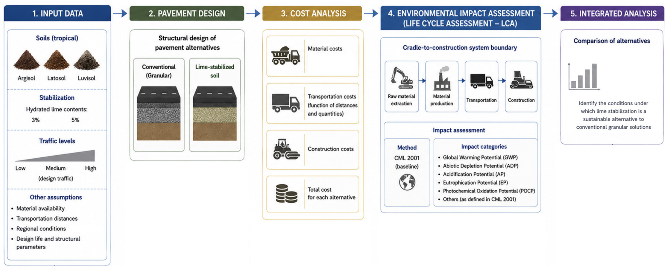
Figure 1. Sustainability-oriented methodological framework for pavements with lime-stabilized soils.
Infrastructures 11 00301 g001
Figure 2. System boundaries.
Infrastructures 11 00301 g002
Figure 3. Pavement sections.
Infrastructures 11 00301 g003
Figure 4. Environmental impacts for Argisol subgrade.
Infrastructures 11 00301 g004
Figure 5. Environmental impacts for Latosol subgrade.
Infrastructures 11 00301 g005
Figure 6. Environmental impacts for Luvisol subgrade.
Infrastructures 11 00301 g006
Figure 7. Relative global warming potential for Argisol.
Infrastructures 11 00301 g007
Figure 8. Relative global warming potential for Latosol.
Infrastructures 11 00301 g008
Figure 9. Relative global warming potential for Luvisol.
Infrastructures 11 00301 g009
Figure 10. Relative cost and global warming potential emissions versus traffic level for Argisol, Latosol, and Luvisol subgrades.
Infrastructures 11 00301 g010
Table 1. Geotechnical and chemical properties of the soils.
ArgisolLatosolLuvisol
Geotechnical properties
% passing the #200 sieve [48]539595
Plasticity index, PI (%) [49]171528
Specific density, ρ (g/cm3) [50]2.6753.0342.702
Poisson’s ratio0.400.400.40
Classification
AASHTO [51]A-7-5A-7-5A-7-5
USCS [52]MLMHMH
MCT [53]NS’LG’NG’
Chemical properties 1
pH (H2O)5.14.66.8
P (mg/dm3)0.20.717
K (mg/dm3)6.051>400
Alexchangeable (cmolc/dm3)1.20.80.0
CEC (cmolc/dm3)2.67.327.3
Organic matter (%)0.20.71.5
Base saturation (%)163394
1 The chemical characterization was carried out following the procedures established by the Official Network of Soil and Plant Tissue Analysis Laboratories of Rio Grande do Sul and Santa Catarina (ROLAS), which provides standardized analytical methods widely used in Brazil for soil chemical characterization and fertility assessment [54].
Table 2. Resilient modulus model parameters and statistical significance [47].
k1k2k3RM Model
(MPa)
SR2
Argisol1130.232−0.297 R M = k 1 σ 3 k 2 σ d k 3 12.0000.670
Latosol2000.431−0.28013.5000.660
Luvisol34−0.063−0.39815.3000.880
RM: resilient modulus; σ3: confining stress; σd: deviator stress; S: variance; R2: coefficient of determination.
Table 3. Physical and mechanical properties of soil–lime mixtures [47].
SoilLime Content (%)Compactive Effortγd (kN/m3) OMC (%)Modulus
(MPa)
Poisson’s RatioUCS28 days
(MPa)
ԑb
(Microstrain)
Argisol3Modified18.2513.237720.202.930207
Argisol5Modified18.0513.548400.203.400213
Latosol3Modified15.2528.410470.201.320174
Latosol5Modified15.0029.814990.202.170196
Luvisol3Standard13.9129.26820.200.410192
Luvisol5Standard13.8728.49030.200.500270
γd: maximum dry unit weight [58]; OMC: optimum moisture content [58]; modulus [59,60]; Poisson’s ratio [16,61,62] UCS28 days: unconfined compressive strength [63]; ԑb: strain at break [59,60].
Table 4. Design parameters for granular materials.
Materialγd (kN/m3)ModulusPoisson’s Ratio
μ
Linear
(MPa)
Model
(MPa)
k1k2 R M = k 1 σ 3 k 2
Graded crushed stone 119.6-22060.7300.35
Macadam 217.7250-- 0.35
γd: dry unit weight.; 1 [64]; 2 [65]. RM: resilient modulus; σ3: confining stress.
Table 5. Mix proportions for asphalt mixtures.
MaterialCompositionQuantityUnit
Asphalt Mixture—Range BFine aggregate0.363t
Fine crushed stone #00.083t
Crushed stone #10.267t
Filler–hydrated lime0.052t
Binder–Pen 50/700.057t
Small-sized crushed stone0.174t
Asphalt Mixture—Range CFine aggregate0.487t
Fine crushed stone #00.090t
Crushed stone #10.094t
Filler–hydrated lime0.056t
Binder–Pen 50/700.006t
Small-sized crushed stone0.206t
Mix proportions adopted from the Brazilian Cost Reference System [69].
Table 6. Process modeling for the product stage (A1–A3).
ProcessInput 1Background Data
Base/subbase coursesHydrated limehydrated lime production, loose|hydrated lime, loose|cutoff, U-RoW
Graded crushed stone/macadamgravel production, crushed|gravel, crushed|cutoff, U-BR
Prime coatCut-back asphaltbitumen adhesive compound production, hot|bitumen adhesive compound, hot|cutoff, U-RoW
Tack coatAsphalt emulsionbitumen seal production|bitumen seal|Cutoff, U-RoW
HMAAsphalt binderbitumen adhesive compound production, hot|bitumen adhesive compound, hot|cutoff, U-RoW
Transport of asphalt binder to the plantmarket for transport, freight, lorry, 7.5–16 metric ton, diesel, EURO 5|transport, freight, lorry, 7.5–16 metric ton, diesel, EURO 5|cutoff, U-BR
Coarse aggregategravel production, crushed|gravel, crushed|Cutoff, U-BR
Transport of coarse aggregate to the plantmarket for transport, freight, lorry, 7.5–16 metric ton, diesel, EURO 5|transport, freight, lorry, 7.5–16 metric ton, diesel, EURO 5|cutoff, U-BR
Fine aggregategravel and sand quarry operation|sand|Cutoff, U-RoW
Transport of fine aggregate to the plantmarket for transport, freight, lorry, 7.5–16 metric ton, diesel, EURO 5|transport, freight, lorry, 7.5–16 metric ton, diesel, EURO 5|cutoff, U-BR
Fillersand to generic market for inert filler|inert filler|Cutoff, U-GLO
Transport of filler to the plantmarket for transport, freight, lorry, 7.5–16 metric ton, diesel, EURO 5|transport, freight, lorry, 7.5–16 metric ton, diesel, EURO 5|cutoff, U-BR
Diesel for HMA production 2market for diesel, burned in building machine|diesel, burned in building machine|cutoff, U-GLO
Electricity for HMA production 3market for electricity, medium voltage|electricity, medium voltage|cutoff, U-BR-Southern grid
1 Foreground data follows pavements’ specificities shown in Tables 11–14; 2 66 kwh/t of HMA; 3 4.92 kWh/t of HMA; 2,3 estimated based on the reference guide Brazilian Cost Reference System [69].
Table 7. Transport distances.
SubgradeHMA to the Field
(km)
Hydrated Lime to the Field
(km)
Coarse Aggregate to the Field (km)Asphalt Binder to the Plant
(km)
Coarse Aggregate to the Plant (km)Fine Aggregate to the Plant (km)Filler to the Asphalt Plant
(km)
Argisol50160201303030130
Luvisol501402090303090
Latosol502902040303040
Table 8. Process modeling for the transport stage (A4).
ProcessInput 1Background Data
Transport to the fieldTransport of coarse aggregate to the fieldMarket for transport, freight, lorry, 7.5–16 metric ton, diesel, EURO 5|transport, freight, lorry, 7.5–16 metric ton, diesel, EURO 5|Cutoff, U-BR
Transport of hydrated lime to the field
Transport of HMA to the field
Transport of cut-back asphalt to the field
Transport of asphalt emulsion to the field
1 Foreground data follow the transport distances shown in Table 7 and pavements’ specificities shown in Tables 11–14.
Table 9. Process modeling for the construction stage (A5).
ProcessInput 1Background Data
Pavement constructionEnergy for soil–lime layer construction
(soil–lime)
market for diesel, burned in building machine|diesel, burned in building machine|cutoff, U-GLO
Energy for granular layer construction
(macadam)
Energy for granular layer construction
(graded crushed stone)
Energy for prime coating
Energy for tack coating
Energy for HMA paving and compaction
1 Foreground data follow the pavements’ specificities shown in Tables 11–14 and energy consumption presented in Table 10.
Table 10. Energy consumption and equipment set considered for the construction stage (A5).
Construction ServiceEnergy
Consumption 1
Equipment Set
Soil–lime layer construction
(soil–lime)
4.87 kWh/m3 cement and lime spreading truck, 17 m3 (210 kW)
tanker truck, 10,000 L (188 kW)
motor grader (93 kW)
self-propelled pneumatic-tire roller, 27-ton (85 kW)
self-propelled vibratory sheepsfoot roller, 11.6-ton (82 kW)
agricultural tractor on pneumatic tires (77 kW)
Granular layer construction
(macadam)
2.35 kWh/m3self-propelled pneumatic-tire aggregate spreader (130 kW)
self-propelled vibratory smooth drum roller, 11-ton (97 kW)
Granular layer construction
(graded crushed stone)
4.42 kWh/m3self-propelled aggregate spreader (130 kW)
pneumatic-tire roller, 27-ton (85 kW)
vibratory smooth drum roller, 11-ton (97 kW)
Prime coating0.12 kWh/m2asphalt distributor tanker truck, 6000 L (7 kW/136 Kw)
Tack coating0.09 kWh/m2asphalt distributor tanker truck, 6000 L (7 kW/136 Kw)
HMA paving and compaction2.50 kWh/tself-propelled pneumatic-tire roller, 27-ton (85 kW)
self-propelled vibratory tandem roller, 10.4-ton (82 kW)
tracked asphalt paver (82 kW)
1 Estimated based on the Brazilian Cost Reference System [69].
Table 11. Pavement sections for unbound structures.
SoilN
(Design) 1
Asphalt Layer
(Upper + Lower) 2
(cm)
Number of Layers
(Upper + Lower) 2
ESALs
(to Failure)
Failure Mechanism
ArgisolN19.5 (5.5 + 4)1 + 11.30 × 10⁶fatigue of the lower asphalt layer
N212 (8 + 4)2 + 16.47 × 10⁶fatigue of the lower asphalt layer
N313 (9 + 4)2 + 11.16 × 10⁷fatigue of the lower asphalt layer
N417.5 (13.5 + 4)2 + 17.11 × 10⁷fatigue of the upper asphalt layer
N519.5 (15.5 + 4)3 + 11.03 × 10⁸fatigue of the upper asphalt layer
LuvisolN19 (5 + 4)1 + 11.05 × 10⁶fatigue of the lower asphalt layer
N211.5 (7.5 + 4)2 + 15.63 × 10⁶fatigue of the lower asphalt layer
N313 (9 + 4)2 + 11.33 × 10⁷fatigue of the lower asphalt layer
N417 (13 + 4)2 + 15.23 × 10⁷fatigue of the upper asphalt layer
N520 (16 + 4)3 + 11.39 × 10⁸fatigue of the upper asphalt layer
LatosolN110 (6 + 4)1 + 11.63 × 10⁶fatigue of the lower asphalt layer
N212 (8 + 4)2 + 15.75 × 10⁶fatigue of the lower asphalt layer
N313 (9 + 4)2 + 11.02 × 10⁷fatigue of the lower asphalt layer
N418 (14 + 4)2 + 15.99 × 10⁷fatigue of the upper asphalt layer
N520 (16 + 4)3 + 11.13 × 10⁸fatigue of the upper asphalt layer
1 N (design): N1: 1.00 × 10⁶, N2: 5.00 × 10⁶, N3: 1.00 × 10⁷, N4: 5.00 × 10⁷, N5: 1.00 × 10⁸; 2 upper layer: (RM 8000 MPa, DNIT Range C) + lower layer (RM 3000 MPa, DNIT Range B).
Table 12. Pavement sections designed for the Argisol subgrade.
Lime Content (%)N
(Design) 1
Asphalt Layer
(Upper + Lower) 2
(cm)
Number of Layers
(Upper + Lower) 2
Soil–Lime Layer Thickness (cm)ESALs
(to Failure)
Failure Mechanism
3N141201.47 × 107fatigue of the cemented layer
N241201.47 × 107fatigue of the cemented layer
N341201.47 × 107fatigue of the cemented layer
N492305.21 × 107fatigue of the cemented layer
N512 (8 + 4)2 + 1401.26 × 108crushing of the cemented layer
5N141201.77 × 107fatigue of the cemented layer
N241201.77 × 107fatigue of the cemented layer
N341201.77 × 107fatigue of the cemented layer
N461305.09 × 107crushing of the cemented layer
N511 (7 + 4)1 + 1401.12 × 108crushing of the cemented layer
1 N (design): N1: 1.00 × 10⁶, N2: 5.00 × 10⁶, N3: 1.00 × 10⁷, N4: 5.00 × 10⁷, N5: 1.00 × 10⁸; 2 Design 1: upper layer (RM 3000 MPa, DNIT Range B) + lower layer: not applicable; Design 2: upper layer: (RM 8000 MPa, DNIT Range C) + lower layer (RM 3000 MPa, DNIT Range B).
Table 13. Pavement sections designed for the Latosol subgrade.
Lime
Content (%)
N
(Design) 1
Asphalt Layer
(Upper + Lower) 2
(cm)
Number of Layers
(Upper + Lower) 2
Soil–Lime Layer Thickness (cm)ESALs
(to Failure)
Failure Mechanism
3N141201.32 × 106crushing of the cemented layer
N2102205.58 × 106fatigue of the cemented layer
N392301.03 × 107crushing of the cemented layer
N413 (9 + 4)2 + 1405.86 × 107crushing of the cemented layer
N519 (15 + 4)3 + 1401.00 × 108fatigue of the cemented layer
5N141204.82 × 106fatigue of the cemented layer
N251205.59 × 106fatigue of the cemented layer
N341251.16 × 107fatigue of the cemented layer
N49 (5 + 4)1 + 1405.32 × 107crushing of the cemented layer
N514 (10 + 4)2 + 1401.03 × 108fatigue of the cemented layer
1 N (design): N1: 1.00 × 10⁶, N2: 5.00 × 10⁶, N3: 1.00 × 10⁷, N4: 5.00 × 10⁷, N5: 1.00 × 10⁸; 2 Design 1: upper layer (RM 3000 MPa, DNIT Range B) + lower layer: not applicable; Design 2: upper layer: (RM 8000 MPa, DNIT Range C) + lower layer (RM 3000 MPa, DNIT Range B).
Table 14. Pavement sections designed for the Luvisol subgrade.
Lime Content (%)N
(Design) 1
Asphalt Layer
(Upper + Lower) 2
(cm)
Number of Layers
(Upper + Lower) 2
Soil–Lime Layer Thickness (cm)ESALs
(to Failure)
Failure Mechanism
3N1102201.00 × 106fatigue of the cemented layer
N211 (7 + 4)1 + 1207.94 × 106fatigue of the cemented layer
N312 (8 + 4)2 + 1201.40 × 107fatigue of the cemented layer
N416 (12 + 4)2 + 1305.95 × 107fatigue of the cemented layer
N519 (15 + 4)3 + 1401.06 × 108crushing of the cemented layer
5N141201.04 × 106fatigue of the cemented layer
N28 (4 + 4)1 + 1202.86 × 107fatigue of the cemented layer
N38 (4 + 4)1 + 1202.86 × 107fatigue of the cemented layer
N416 (12 + 4)2 + 1306.72 × 107fatigue of the cemented layer
N517 (13 + 4)2 + 1401.04 × 108fatigue of the cemented layer
1 N (design): N1: 1.00 × 10⁶, N2: 5.00 × 10⁶, N3: 1.00 × 10⁷, N4: 5.00 × 10⁷, N5: 1.00 × 10⁸; 2 Design 1: upper layer (RM 3000 MPa, DNIT Range B) + lower layer: not applicable; Design 2: upper layer: (RM 8000 MPa, DNIT Range C) + lower layer (RM 3000 MPa, DNIT Range B).
Table 15. Relative environmental impacts of pavements with soil–lime and the respective pavements with granular layers for Argisol subgrade.
3% Lime5% Lime
N1N2N3N4N5N1N2N3N4N5
Ozone depletion0.370.300.290.480.620.390.320.310.350.59
Abiotic depletion (fossil fuels)0.380.310.290.490.630.400.330.310.360.60
Abiotic depletion (elements)0.330.270.260.430.570.340.280.270.290.51
Global warming potential (GWP)0.570.500.480.730.940.750.660.630.781.12
Photochemical oxidation0.330.300.290.490.640.400.360.340.440.68
Acidification0.230.210.210.380.500.260.240.230.310.50
Freshwater aquatic ecotoxicity0.330.280.270.460.600.360.310.290.340.57
Marine aquatic ecotoxicity0.380.320.310.500.650.440.370.350.420.66
Terrestrial ecotoxicity0.500.410.390.600.770.620.510.480.560.84
Eutrophication0.250.220.220.390.510.270.240.230.280.47
Human toxicity0.350.300.290.490.650.390.340.320.390.63
Table 16. Relative environmental impacts of pavements with soil–lime and the respective pavements with granular layers Latosol subgrade.
3% Lime5% Lime
N1N2N3N4N5N1N2N3N4N5
Ozone depletion0.360.690.620.720.930.380.390.320.550.73
Abiotic depletion (fossil fuels)0.360.710.620.730.940.380.390.320.550.73
Abiotic depletion (elements)0.330.610.560.690.860.360.340.300.520.67
Global warming potential (GWP)0.520.800.830.991.180.670.660.671.021.17
Photochemical oxidation0.310.580.560.700.890.370.380.360.610.77
Acidification0.220.450.420.540.720.250.270.240.440.59
Freshwater aquatic ecotoxicity0.320.610.560.690.880.350.360.310.540.70
Marine aquatic ecotoxicity0.360.650.610.740.930.420.410.380.620.78
Terrestrial ecotoxicity0.470.770.740.871.050.570.540.520.800.94
Eutrophication0.250.490.460.590.760.280.290.260.460.61
Human toxicity0.340.630.590.730.930.380.380.340.590.76
Table 17. Relative environmental impacts of pavements with soil–lime and the respective pavements with granular layers for Luvisol subgrade.
3% Lime5% Lime
N1N2N3N4N5N1N2N3N4N5
Ozone depletion0.950.880.891.050.970.480.690.630.960.89
Abiotic depletion (fossil fuels)0.960.900.901.060.980.480.700.640.970.90
Abiotic depletion (elements)0.860.760.830.950.900.450.630.590.880.79
Global warming potential (GWP)1.010.970.981.291.210.770.920.861.271.30
Photochemical oxidation0.810.790.811.020.980.530.690.650.970.96
Acidification0.710.700.720.900.880.470.600.580.840.84
Freshwater aquatic ecotoxicity0.850.800.831.000.940.470.660.610.920.87
Marine aquatic ecotoxicity0.900.840.871.050.980.540.710.660.980.94
Terrestrial ecotoxicity1.030.940.951.171.070.670.830.771.121.07
Eutrophication0.730.690.740.890.870.440.590.560.830.79
Human toxicity0.830.790.831.020.970.470.660.620.950.91
Table 18. Normalized life-cycle impacts on ecosystem quality.
Life-Cycle Impact CategoryNormalization Factor *Ecosystem Quality **
ArgisolLatosolLuvisol
Granular5% LimeGranular5% LimeGranular5% Lime
Acidification3.93 × 101445015674402165144282936
Eutrophication2.61 × 101
Terrestrial Ecotoxicity1.80 × 102
Fresh Water Aquatic Toxicity3.90 × 102
Marine Aquatic Ecotoxicity3.22 × 104
Global Warming GWP 100a6.96 × 103
* Based on the CML–IA impact assessment spreadsheet available for download at https://www.universiteitleiden.nl/en/research/research-output/science/cml-ia-characterisation-factors#downloads (accessed on 1 May 2026); world 2000—most recent data available; ** results corresponding to the functional unit (1 km of pavement, consisting of two 3.5 m-wide traffic lanes, including the subbase, base, and surface layers).
Table 19. Normalized life-cycle impacts on human health.
Life-Cycle Impact CategoryNormalization Factor *Human Health **
ArgisolLatosolLuvisol
Granular5% LimeGranular5% LimeGranular5% Lime
Global Warming GWP 100a6.96 × 103589204584214587374
Human Toxicity4.25 × 102
Photochemical Oxidation6.07 × 100
Ozone Depletion3.73 × 10−2
* Based on the CML–IA impact assessment spreadsheet available for download at https://www.universiteitleiden.nl/en/research/research-output/science/cml-ia-characterisation-factors#downloads (accessed on 1 May 2026); world 2000—most recent data available; ** results corresponding to the functional unit (1 km of pavement, consisting of two 3.5 m-wide traffic lanes, including the subbase, base, and surface layers).
Table 20. Normalized life-cycle impacts on resources.
Life-Cycle Impact CategoryNormalization Factor *Resources **
ArgisolLatosolLuvisol
Granular5% LimeGranular5% LimeGranular5% Lime
Abiotic depletion (elements)5.95 × 10−21605015951159101
Abiotic depletion (fossil fuels)6.26 × 10⁴
* Based on the CML–IA impact assessment spreadsheet available for download at https://www.universiteitleiden.nl/en/research/research-output/science/cml-ia-characterisation-factors#downloads (accessed on 1 May 2026); world 2000—most recent data available; ** results corresponding to the functional unit (1 km of pavement, consisting of two 3.5 m-wide traffic lanes, including the subbase, base, and surface layers).
Disclaimer/Publisher’s Note: The statements, opinions and data contained in all publications are solely those of the individual author(s) and contributor(s) and not of MDPI and/or the editor(s). MDPI and/or the editor(s) disclaim responsibility for any injury to people or property resulting from any ideas, methods, instructions or products referred to in the content.