Point-Cloud-Based 3D Inspection and Volume Quantification of Drainage-Pipeline Defects Using WCPC-GAN and Density-Adaptive Alpha Shapes

Abstract

Closed-circuit television (CCTV)-based inspection provides limited depth information and cannot directly quantify the three-dimensional geometry of drainage-pipeline defects. Moreover, the scarcity of annotated point-cloud data and the topological artifacts produced by conventional surface-reconstruction methods hinder automated condition assessment. This study presents a point-cloud-based framework for 3D inspection and volume quantification of concrete drainage-pipeline defects. WCPC-GAN expands the available defect data; PointNeXt segments the point clouds; and a RANSAC-constrained, density-adaptive Alpha Shape method reconstructs the defect surface for volume integration. The framework was evaluated using 15 independently fabricated circular, triangular, and rectangular defects, with reference volumes obtained through repeated water-displacement measurements. The proposed reconstruction achieved mean volume accuracies of 96.32 ± 0.67%, 96.78 ± 0.60%, and 96.86 ± 0.37%, respectively, and exceeded a contemporary CAP-UDF baseline by 1.62, 2.68, and 3.06 percentage points. Paired-bootstrap analysis estimated an overall error reduction of 5.56 percentage points over conventional Alpha Shape (95% confidence interval: 5.17–5.97). Synthetic augmentation also increased PointNeXt performance on the fixed real-only test set from 92.52% accuracy and 83.53% mIoU to 94.53% and 89.98%, respectively. The results support physically calibrated defect-volume assessment under controlled experimental conditions.

1. Introduction

Urban drainage pipelines constitute critical lifelines of underground infrastructure systems, directly influencing urban safety, environmental quality, public service reliability, and system resilience. Concrete pipelines are prone to structural deterioration under long-term hydraulic, mechanical, and chemical interactions. Defects such as cracking, spalling, cavities, and joint dislocations are often concealed and progressive; if not detected and assessed in time, they can contribute to leakage, soil erosion, and road collapse [1,2,3]. Accurate inspection and quantitative evaluation are therefore central to drainage-pipeline condition assessment.

Traditionally, pipeline inspection has relied on techniques such as Closed-Circuit Television (CCTV), sonar, and Ground-Penetrating Radar (GPR) [4,5,6,7]. While CCTV provides intuitive visual data, it lacks depth information, making it impossible to measure the volumetric dimensions of defects. Sonar is limited to submerged conditions with low resolution, while GPR faces trade-offs between detection depth and precision. Consequently, these two-dimensional or indirect sensing methods are insufficient for accurately characterizing complex defect geometries. With the development of laser scanning and multi-view geometry techniques, 3D point cloud data have emerged as a superior representation for inspection [8,9]. Their high spatial resolution and geometric expressiveness provide a solid foundation for capturing the detailed inner-surface geometry of pipelines.

1.1. Related Works

To interpret these unstructured point clouds for automated inspection, semantic segmentation—assigning a semantic label to each point—is the prerequisite step. Deep learning methods have been increasingly applied to point-cloud segmentation. Representative architectures such as PointNet++ [10] and DGCNN [11] have shown effective feature-learning capabilities for unstructured 3D data. Recent studies have further adapted these models to underground-infrastructure inspection. For instance, Zhang et al. [12] combined deep feature learning with geometric consistency to segment curved pipelines and measure gaps in industrial settings. Cui et al. [13] developed a cross-scale network to enhance defect recognition in low-quality underwater sonar point clouds. Furthermore, Wang et al. [14] integrated Feature Pyramid Networks (FPN) to optimize defect classification boundaries. These studies indicate that deep learning-based segmentation has become a viable and effective tool for pipeline feature extraction.

However, despite these architectural advancements, the practical deployment of intelligent inspection systems for concrete pipelines faces two critical challenges that remain underexplored.

The first challenge concerns data scarcity and the limitations of existing augmentation strategies. Deep-learning models typically require large annotated datasets to achieve reliable generalization. Compared with autonomous-driving benchmarks such as KITTI, publicly available point-cloud datasets for concrete drainage pipelines remain scarce because data acquisition in confined and potentially hazardous environments is difficult and annotation is labor-intensive [14,15]. This problem is especially pronounced for non-man-entry pipelines, where the deployment of large terrestrial laser-scanning systems is impractical. In this study, five DN1200 prefabricated concrete pipes were used to establish a controlled experimental platform. The relatively large pipe diameter facilitated defect fabrication, stable point-cloud acquisition, and repeated physical volume measurements; however, the platform does not fully reproduce the restricted acquisition conditions encountered in smaller operational pipelines. This limitation is therefore considered in the discussion of field generalization. Conventional augmentation techniques, such as rotation and scaling, can increase sample variation but cannot adequately reproduce the diverse local geometries of pipeline defects. Although generative adversarial networks have been investigated for point-cloud synthesis [16,17,18], many existing approaches still face a trade-off between computational efficiency and geometric fidelity. Some require substantial computational resources, whereas others may not adequately preserve the fine-scale local structures, such as the sharp boundaries of concrete spalling, required for engineering-oriented analysis [19].

The second challenge lies in the gap between semantic segmentation results and precise quantitative evaluation. Obtaining semantic labels is not the final goal of inspection; engineering maintenance decisions depend on quantitative metrics, such as defect volume, depth, and surface area [20]. Direct calculation from segmented point clouds is prone to significant errors due to point sparsity, geometric occlusion, and sensor outliers. Therefore, 3D surface reconstruction is essential to recover the continuous topology of defects. Standard implicit methods like Poisson reconstruction [21] or Alpha Shape algorithms [22] typically assume global smoothness or uniform density. When applied to the irregular, broken geometries of concrete defects, these methods frequently result in topological artifacts (e.g., holes) or over-smoothed boundaries, leading to inaccurate volume estimation. Moreover, they often require tedious manual parameter tuning, hindering automated processing [23].

In summary, existing point-cloud-based pipeline inspection methods face three interconnected limitations. First, the limited availability of annotated defect point clouds restricts the development of reliable data-driven segmentation models. Second, conventional surface reconstruction methods commonly employ globally fixed parameters and therefore cannot adequately accommodate spatial variations in point-cloud density, resulting in fragmented surfaces, blurred boundaries, or topological artifacts. Third, semantic segmentation results are rarely connected to physically validated engineering quantities, such as defect volume, which limits their direct value for infrastructure condition assessment and maintenance planning.

To address these limitations, this study develops an integrated point-cloud framework that connects defect-data augmentation, semantic segmentation, density-adaptive surface reconstruction, and physically validated volume quantification. WCPC-GAN is introduced to expand the limited defect dataset while preserving local geometric characteristics. The segmented point clouds are then reconstructed using a method that combines cylindrical geometric constraints, Delaunay triangulation, and local-density-driven Alpha Shape optimization. Finally, the calculated defect volumes are compared with physical reference measurements obtained using the water-displacement method. In this manner, the proposed framework establishes a processing chain from limited point-cloud data to engineering-oriented quantitative defect assessment.

1.2. Main Contributions

To address the limitations of data scarcity, irregular defect geometry, and insufficient quantitative assessment in drainage-pipeline inspection, this study develops an integrated point-cloud framework connecting data augmentation, semantic segmentation, surface reconstruction, and engineering-oriented volume validation. The main contributions are summarized as follows:

(1)

A lightweight defect point-cloud augmentation method, termed WCPC-GAN, is developed to expand limited annotated pipeline-defect datasets. By incorporating a local warping mechanism into the auxiliary generator, the proposed method strengthens the representation of local geometric details while maintaining a relatively compact model size and reasonable inference efficiency. Compared with representative point-cloud generative models, WCPC-GAN achieved the lowest JSD and MMD-CD and the highest COV-EMD among the compared models, with 3.11 M parameters.

(2)

A density-adaptive surface reconstruction method is proposed for the quantitative reconstruction of irregular drainage-pipeline defects. The method combines RANSAC-based cylindrical fitting, Delaunay triangulation, and local-density-driven Alpha Shape optimization. Unlike conventional Alpha Shape reconstruction using a fixed global parameter, the proposed strategy adapts the reconstruction parameter to local point-cloud density, thereby improving boundary preservation, surface continuity, and topological completeness in defect regions.

(3)

An engineering-oriented validation procedure is established to evaluate defect volume quantification using physically fabricated concrete-pipeline defects. Reference volumes are obtained through repeated water-displacement measurements, enabling direct comparison between reconstructed and physically measured defect volumes. The proposed method achieves mean volume accuracies of 96.3%, 96.8%, and 96.9% for circular, triangular, and rectangular defects, respectively, demonstrating its potential for quantitative condition assessment and maintenance-oriented inspection of drainage-pipeline infrastructure.

2. Materials and Methods

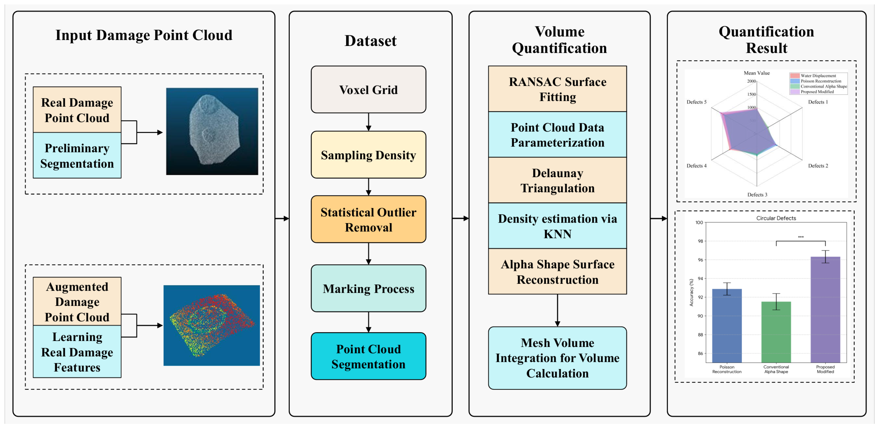
As shown in Figure 1, the framework comprises four stages: WCPC-GAN-based augmentation; PointNeXt segmentation with statistical and normal/curvature refinement; RANSAC-based cylindrical reference fitting and Delaunay meshing; and density-adaptive Alpha Shape reconstruction followed by mesh-volume integration. This sequence connects limited point-cloud data to physically calibrated defect-volume estimates.

2.1. GAN-Based Data Augmentation for Concrete Pipelines

2.1.1. Network Architecture and Local Warping Module Integration

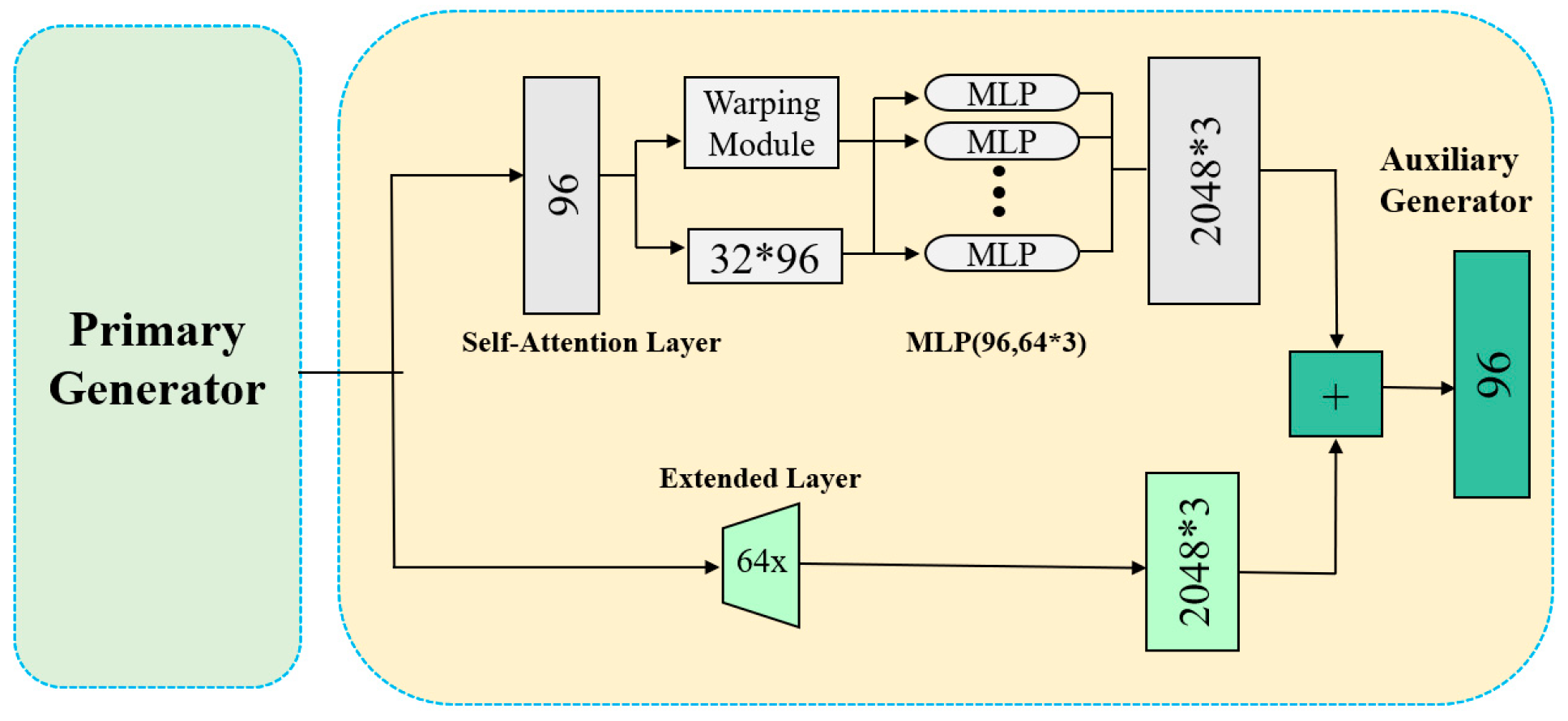
WCPC-GAN extends CPCGAN [16] by embedding the Unified Local-Warping Module [17] in the auxiliary generator. The module uses coarse-to-fine warping to preserve local defect geometry while maintaining global structural coherence.

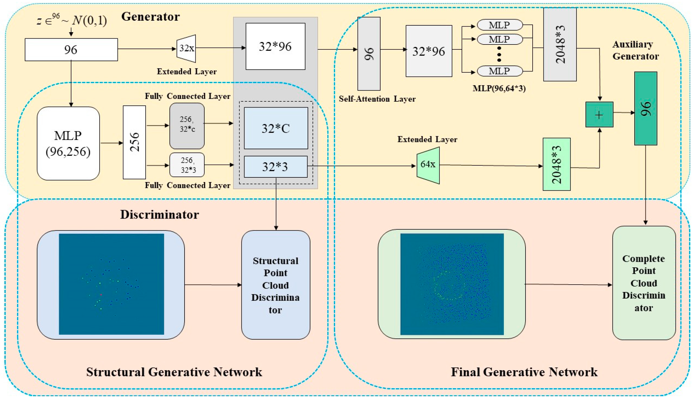
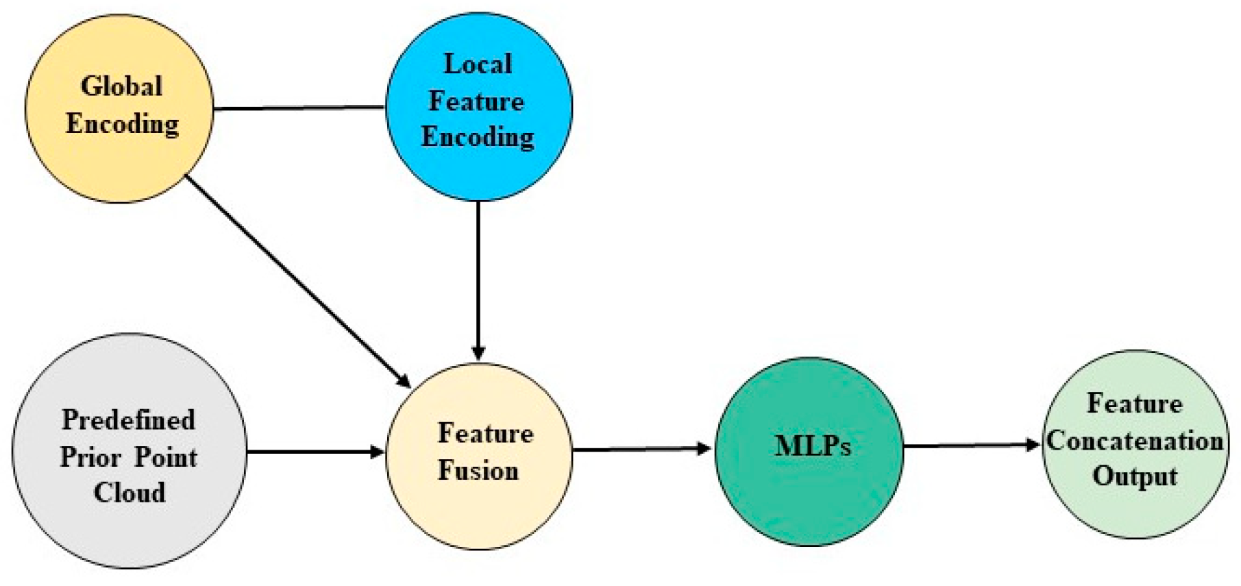
The CPCGAN backbone adopts a two-stage framework comprising a main generator, an auxiliary generator, and a discriminator, as illustrated in Figure 2. The main generator captures the global geometric structure via a Multi-Layer Perceptron (MLP), while to improve the synthesis of local details, we enhance the auxiliary generator by embedding the local warping module derived from WarpingGAN. The specific architectures of the MLP and this enhanced auxiliary generator are detailed in Figure 3 and Figure 4.

The warping module divides the enhancement encoding $\tilde{z}$ equally into $M$ local encodings ${\tilde{z}}^j$ and concatenates them with the global shape information $z^j$ to form a composite encoding $u_i^j$, as described in Equation (1):

$${\left\{{\tilde{z}}^j\in {\mathbb{R}}^{{\displaystyle \frac{D}{M}}}\right\}}_{j=1}^M$$

(1)

To further elevate point cloud generation quality and detail expression, the module executes a two-stage warping operation: first generating a coarse geometric shape, followed by fine-grained optimization. This process involves network parameters ${\Theta }_1$ and ${\Theta }_2$, mathematically expressed in Equation (2):

$$p_i^j=\mathcal{F}\left(\mathcal{F}\left(u_i^j,z^j;{\Theta }_1\right),z^j;{\Theta }_2\right),\forall j\in \left[1,M\right] \mathrm{and} \forall i\in \left[1,n\right]$$

(2)

The two-stage operation refines local defect geometry while preserving global structural coherence.

2.1.2. Loss Function

The model is trained using Wasserstein GAN loss [24] with Gradient Penalty [25] to ensure training stability. To enforce geometric consistency between generated local regions and the global structure, a stitching loss ($L_{\mathrm{WCPCGAN}}$) is introduced. The generator’s combined objective function is defined as:

$$L_{\mathrm{WCPCGAN}}=L_{G_s}+{\lambda }_s{L}_{G_f}+L_{D_s}+{\lambda }_{\mathrm{gp}}{L}_{D_f}$$

(3)

Here, the generators produce structural and complete point clouds, while the corresponding discriminators distinguish generated samples from real samples in the structural and complete domains. The stitching loss minimizes local boundary discrepancies so that defect details remain geometrically consistent with the global pipe structure. The selected setting was λstitch = 0.50 and λGP = 10; its quantitative evaluation is reported in Section 3.1.2.

2.2. Density-Adaptive Defect Surface Reconstruction and Volume Quantification

2.2.1. Cylindrical Equation-Based Surface Fitting

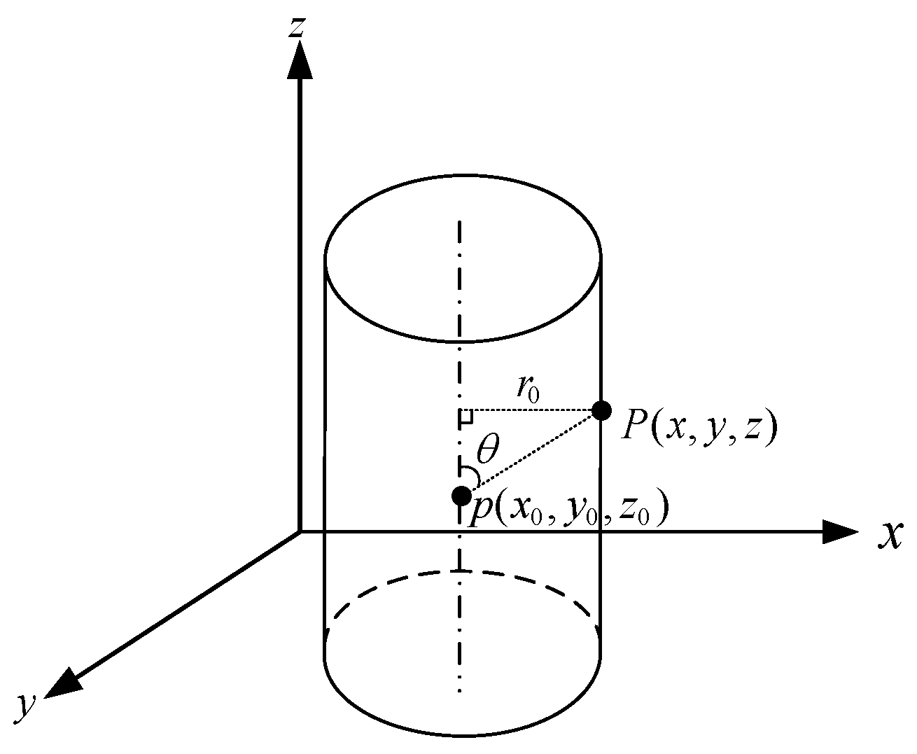
The regular cylindrical geometry of the pipe wall is used as a reference surface. A RANSAC cylinder [26] is parameterized by a point p₀ on its axis, a unit axis vector a, and a radius r₀. For an observed point p_i, the radial distance r_i is obtained after removing the axial component of p_i − p₀, and the cylinder residual e_i is the absolute difference between r_i and r₀, as defined in Equation (4).

$$\begin{array}{ll}{r}_i& =‖(p_i-p_0)-\left[\right(p_i-p_0)·a]a‖\\ e_i& =\left|r_i-r_0\right|\end{array}$$

(4)

A point is classified as a cylinder inlier when its radial residual satisfies Equation (5). The nominal distance threshold was δ₀ = 2.5 mm. This residual definition directly evaluates distance from the fitted cylindrical surface rather than distance from the cylinder axis.

$$e_i\le {\delta }_0,{\delta }_0=2.5 \mathrm{mm}$$

(5)

The nominal threshold was applied consistently to cylinder fitting for all physical specimens. Its influence on the complete downstream volume-quantification pipeline is evaluated through the ±20% sensitivity analysis reported in Section 4.2.

The iteration budget was computed from the standard RANSAC confidence relation and capped at 3000 iterations, as defined in Equation (6).

$$N_{\max }=\mathrm{m}\mathrm{i}\mathrm{n}\left(3000,⌈{\displaystyle \frac{\mathrm{l}\mathrm{n}\left(1-p\right)}{\mathrm{l}\mathrm{n}\left(1-w^s\right)}}⌉\right),p=0.99,s=7$$

(6)

Here, p = 0.99 is the target confidence, w is the current inlier ratio, and s = 7 is the minimum sample size for cylinder fitting. These settings provide a reproducible stopping rule while bounding computation.The fitted cylindrical geometry and its key parameters are illustrated in Figure 5.

2.2.2. Basic Mesh Construction

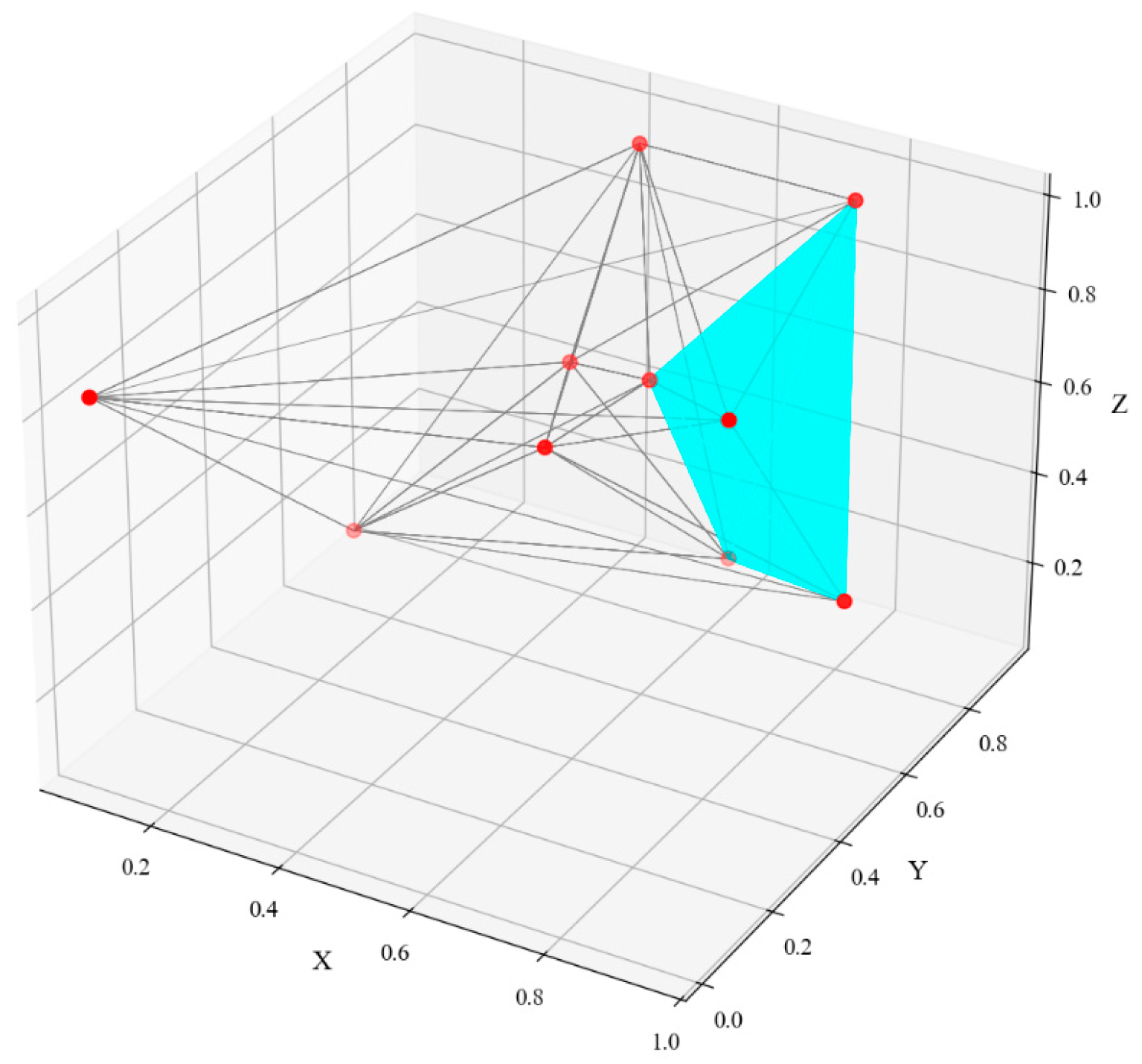
We utilize an incremental Delaunay triangulation algorithm [27] to construct the initial 3D mesh, as shown in Figure 6, which generates a tetrahedral mesh that globally conforms to Delaunay criteria. To efficiently handle large-scale point cloud data, we implement an octree-based spatial partitioning strategy, allowing for parallel local triangulation and subsequent boundary stitching.

2.2.3. Local-Density-Driven Alpha Shape Optimization

Conventional Alpha Shape reconstruction [22] applies one global scale and can therefore lose boundary detail in dense regions or leave gaps in sparse regions. The proposed method assigns a point-neighborhood-level Alpha reference from local point spacing so that the reconstruction scale follows spatial variations in sampling density.

For each point i, a KD-tree [28] identifies its two nearest neighbors. Their Euclidean distances, Sd1,i and Sd2,i, are defined in Equations (7) and (8).

$$S_{d1,i}=\sqrt{{x_{id1}-x_i}^2+{y_{id1}-y_i}^2+{z_{id1}-z_i}^2}$$

(7)

$$S_{d2,i}=\sqrt{{x_{id2}-x_i}^2+{y_{id2}-y_i}^2+{z_{id2}-z_i}^2}$$

(8)

The local spacing Si is defined as the mean of the two nearest-neighbor distances in Equation (9). Smaller values indicate denser sampling and larger values indicate sparser sampling.

$$S_i={\displaystyle \frac{S_{d1,i}+S_{d2,i}}{2}}$$

(9)

Equation (10) maps local spacing to the adaptive Alpha reference. The cloud-level mean spacing defines αref; the normalized local coefficient is ηi = Si/αref; and the point-wise reference is αi = αrefηi. Thus, dense neighborhoods use smaller αi values to preserve boundary detail, whereas sparse neighborhoods use larger values to maintain surface continuity.

$$\begin{array}{cc}{\alpha }_{\mathrm{ref}}& ={\displaystyle \frac{1}{N}}{\displaystyle {\sum }_{i=1}^N}{S}_i\\ {\eta }_i& ={\displaystyle \frac{S_i}{{\alpha }_{\mathrm{ref}}}}\\ {\alpha }_i& ={\alpha }_{\mathrm{ref}}{\eta }_i\end{array}$$

(10)

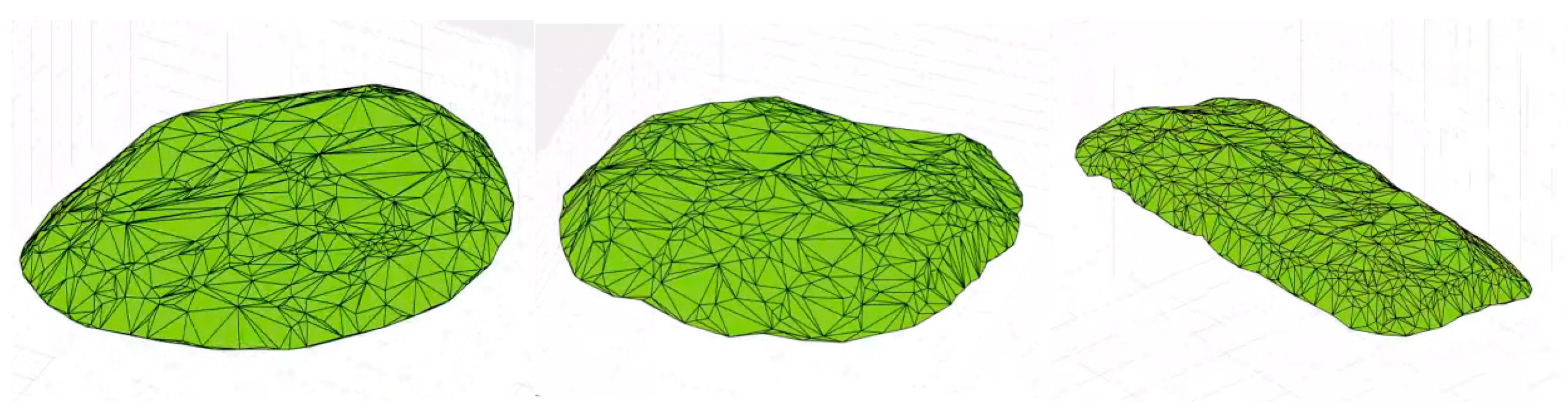
The point-neighborhood-level references express the intended reconstruction-scale variation directly: smaller αi values are associated with dense neighborhoods to preserve local boundary detail, whereas larger αi values are associated with sparse neighborhoods to support surface continuity. Figure 7 illustrates the resulting boundary and surface reconstruction.

3. Experimental Implementation

This study constructs both a real drainage pipeline defect dataset and an augmented drainage pipeline defect dataset. The real defect dataset is collected using the Microsoft Azure Kinect DK depth camera (Microsoft Corporation, Redmond, WA, USA), which provides RGB images with a resolution of 3840 × 2160 pixels and depth images with a resolution of 1024 × 1024 pixels. To enhance the model’s generalization capability, the WCPC-GAN algorithm is applied to augment the collected pipeline dataset based on real drainage pipeline defects. The dataset is divided into two categories based on data sources: the real defect dataset and the augmented defect dataset.

3.1. Dataset Acquisition

3.1.1. Physically Fabricated Dataset

A real dataset comprising 200 point clouds of physically fabricated defects in five DN1200 prefabricated concrete pipes was constructed. The dataset contains 120 circular, 40 rectangular, and 40 triangular defect point clouds acquired with the Microsoft Azure Kinect DK. After voxel-grid down-sampling, curvature-weighted farthest-point sampling was used to standardize each sample to 4000 points. Before any generation or segmentation experiment, the 200 real samples were partitioned into mutually exclusive training, validation, and test subsets at a 3:1:1 ratio (120/40/40). WCPC-GAN was trained using only the 120-sample real training subset; the validation and test subsets were reserved for model selection and final evaluation, respectively.The technical specifications of the Microsoft Azure Kinect DK are summarized in

Table 1. Technical specifications of Microsoft Azure Kinect DK.

Technical Specification	Microsoft Azure Kinect DK
RGB camera resolution	3840 × 2160 pixels
Depth camera resolution	1024 × 1024 pixels
Maximum depth range	5.46 m
Minimum depth range	0.25 m
Vertical field of view	120°
Horizontal field of view	120°

.

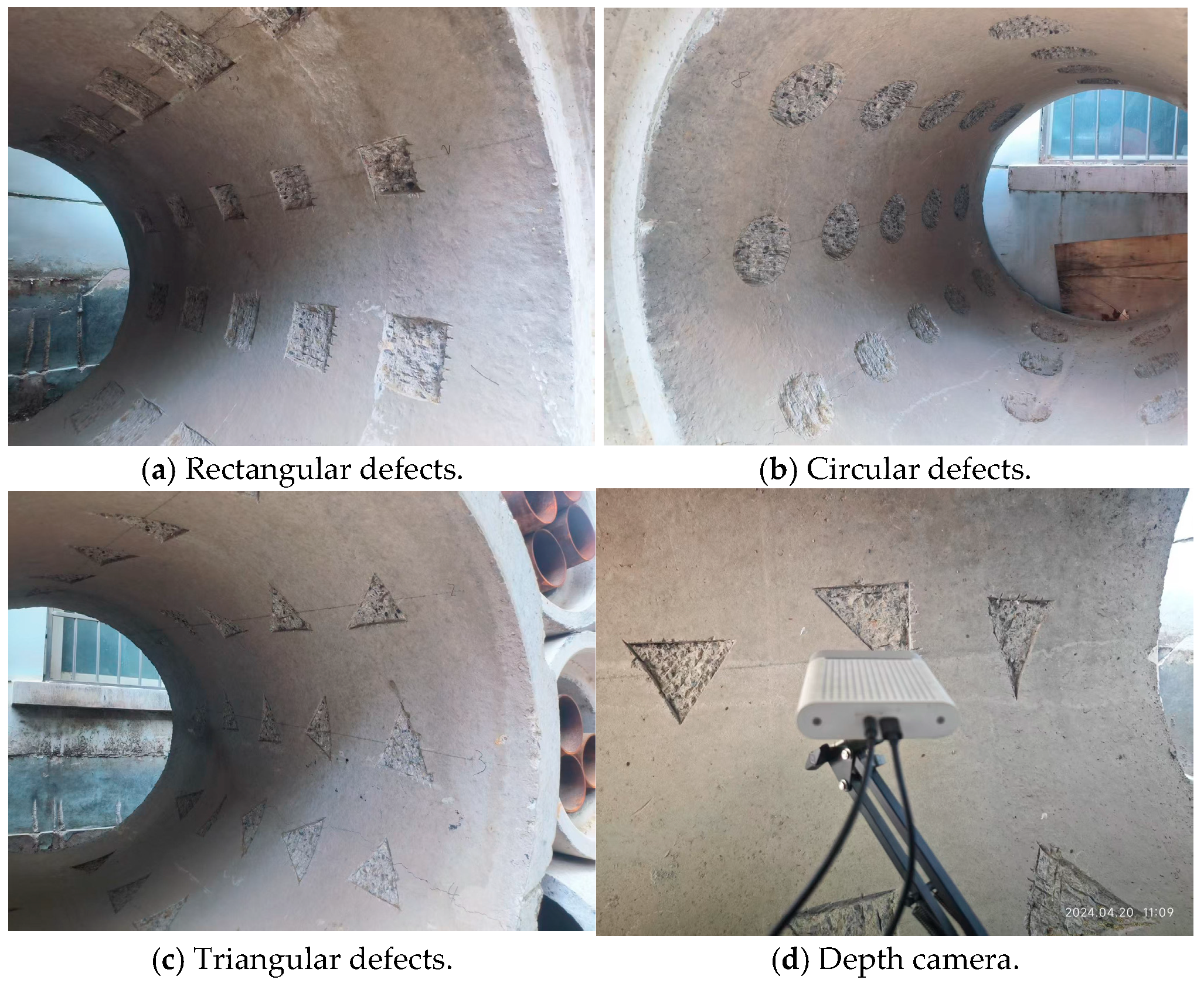
Figure 8a–c presents representative rectangular, circular, and triangular fabricated defects, respectively, while Figure 8d shows the Azure Kinect DK depth camera used for acquisition.

3.1.2. Simulated Dataset

WCPC-GAN was used to generate labeled synthetic defect point clouds for training-set augmentation. The generation experiments were implemented in PyTorch 1.11.0 on Ubuntu 18.04 with an Intel Core i7-11700K CPU and an NVIDIA RTX 2080 Ti GPU. The real validation and test subsets were never used to train WCPC-GAN or PointNeXt.

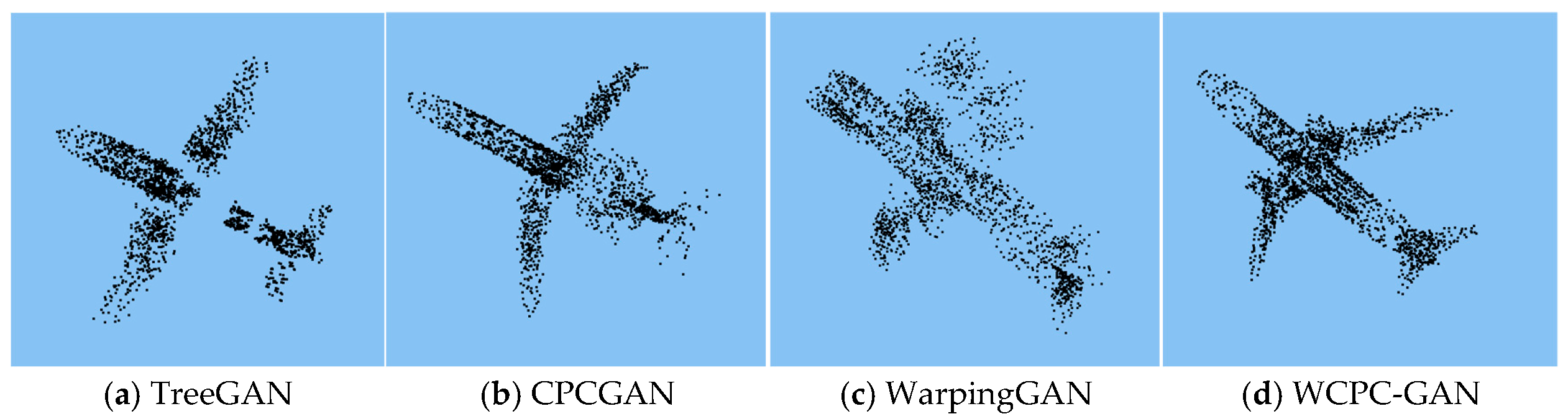
WCPC-GAN was benchmarked against TreeGAN [29], CPCGAN [16], and WarpingGAN [17] using 2690 airplane samples from ShapeNetPart under the same hardware configuration. Performance was evaluated using Jensen–Shannon Divergence (JSD), Minimum Matching Distance (MMD), Coverage (COV), parameter count, and inference time. Figure 9a–d presents representative generated point clouds, and

Table 2. (a) Comparison of WCPC-GAN with point-cloud generative baselines. (b) Sensitivity of WCPC-GAN to loss-weight settings.

(a)
Model		Params (M)	Inference Time (s)		JSD ↓		COV-EMD ↑		MMD-CD ↓
TreeGAN		11.33	9.1		0.0634		46.13		0.00039
CPCGAN		2.14	3.4		0.0416		46.36		0.00036
WarpingGAN		6.34	5.3		0.0571		45.72		0.00043
WCPC-GAN (ours)		3.11	4.9		0.0352		48.63		0.00035
(b)
λstitch	λGP			JSD ↓		COV-EMD ↑		MMD-CD ↓
0.25	10			0.0384		47.61		0.00038
0.50	10			0.0352		48.63		0.00035
1.00	10			0.0368		48.10		0.00036
0.50	5			0.0415		45.30		0.00041
0.50	20			0.0374		47.20		0.00037

Note: ↑ indicates that a higher value is better, whereas ↓ indicates that a lower value is better.

a reports the quantitative comparison.

As shown in Figure 9a–d, WCPC-GAN produced visually complete point clouds with relatively uniform point distributions. Quantitatively, WCPC-GAN achieved the lowest JSD (0.0352) and MMD-CD (0.00035) and the highest COV-EMD (48.63) among the compared methods, while using 3.11 M parameters and an inference time of 4.9 s.

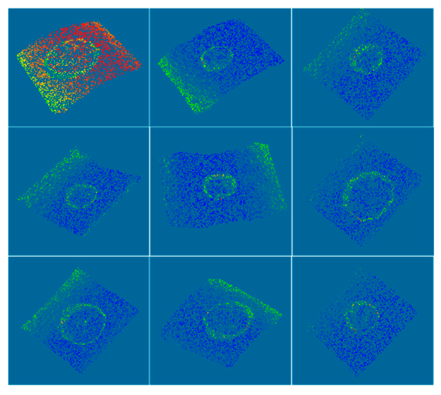
Based on the generative evaluation, 200 labeled synthetic defect models were produced, as illustrated in Figure 10. The real point clouds had an average sampling density of 3.46 points/mm² (346 points/cm²). Each generated cloud was first processed by voxel-grid down-sampling and then by curvature-weighted farthest-point sampling to match this density while retaining defect-boundary detail. Synthetic samples were added exclusively to the 120-sample real training subset. The validation and test sets contained only the fixed 40-sample real subsets; no combined dataset was repartitioned.

The stitching-loss weight and gradient-penalty coefficient were evaluated in five controlled configurations using the same ShapeNetPart data, training schedule, and evaluation protocol as the cross-model comparison. The selected configuration (λ_stitch = 0.50, λ_GP = 10) jointly produced the lowest JSD and MMD-CD and the highest COV-EMD. The configuration was therefore used in the subsequent experiments.

3.2. Dataset Segmentation

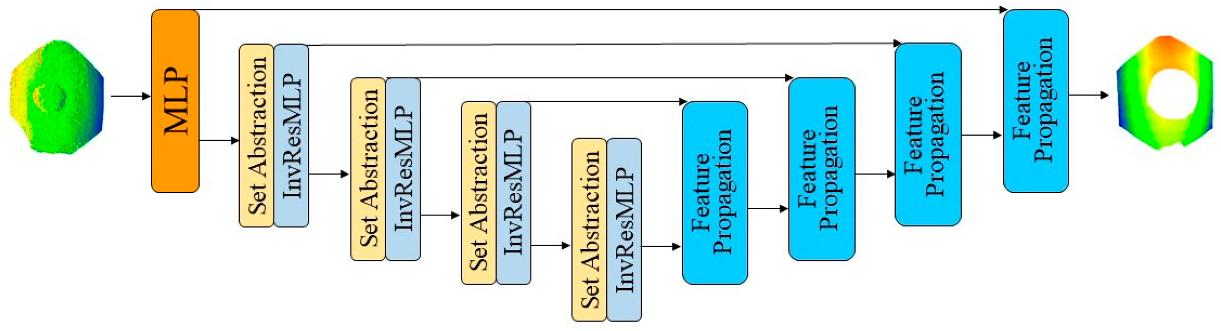
The annotated point clouds were segmented using PointNeXt [30]. PointNeXt revisits PointNet++ training and scaling and uses inverted residual MLP blocks with separable MLPs to strengthen local aggregation efficiently. The encoder progressively extracts neighborhood features through set-abstraction stages, and the decoder propagates multiscale features back to the original points for semantic prediction, as illustrated in Figure 11.

Adding 120 synthetic samples increased accuracy from 92.52% to 94.53% and mIoU from 83.53% to 89.98%, yielding the best performance among the evaluated augmentation settings.

PointNeXt was trained for 300 epochs with a batch size of 16 using AdamW, with an initial learning rate of 1 × 10⁻³, and weight decay of 1 × 10⁻⁴. Training was performed on a 10 GB GeForce RTX 3080 with an Intel i7-8700K CPU and 64 GB RAM under Ubuntu 18.04, Python 3.8, PyTorch 1.11.0, CUDA 11.3, and cuDNN 8.7.

Table 3. Effect of synthetic augmentation on the fixed real-only test set.

Training Set	Accuracy (%)	mIoU (%)
120 real + 0 synthetic	92.52	83.53
120 real + 50 synthetic	92.87	83.49
120 real + 120 synthetic	94.53	89.98
120 real + 200 synthetic	93.46	88.25

evaluates whether synthetic samples improve PointNeXt performance while the 40-sample real validation and 40-sample real test sets remain fixed and synthetic-free.

3.3. Dataset Post-Processing

3.3.1. Statistical Filtering for Low-Density Outlier Removal

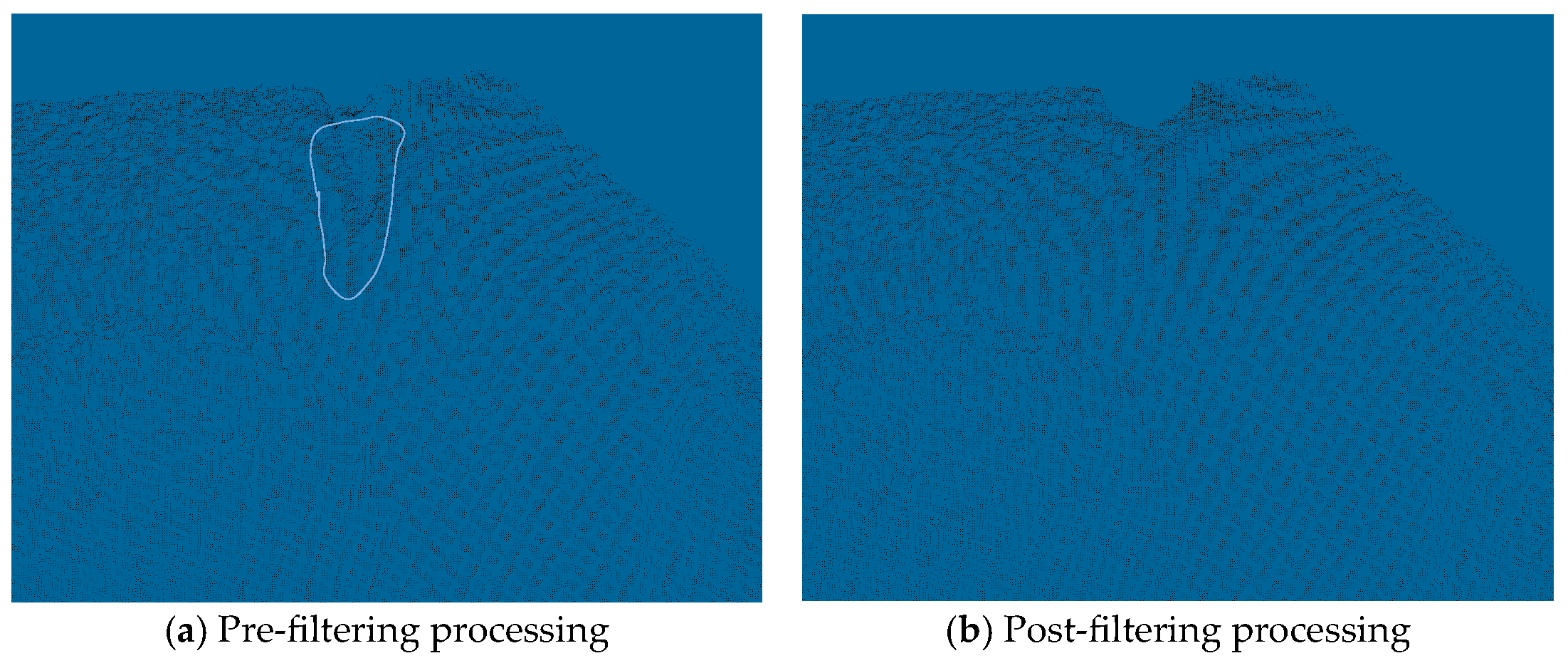
To address prominent outliers caused by measurement noise, statistical filtering based on local point-cloud topology was applied [31]. A KD-tree was used to calculate the mean distance from each point to its k = 50 nearest neighbors. The standard-deviation threshold multiplier was set to 2 under the Gaussian-distance assumption. Points whose mean neighborhood distances exceeded the resulting statistical threshold were classified as low-density outliers and removed. Figure 12 illustrates the point cloud before and after filtering.

3.3.2. Normal-Based and Curvature-Constrained Refinement

Although statistical filtering removes sparse noise, residual anomalies and isolated points may persist, potentially compromising the accuracy of subsequent volume calculations. To further refine the segmentation, particularly for complex defect morphologies, we introduce a normal-based outlier removal strategy constrained by geometric features [32]. For a local neighborhood, we compute the covariance matrix M of the k-nearest neighbors to estimate geometric properties:

$$M={\displaystyle \frac{1}{k}}{\displaystyle {\sum }_{i=1}^k}\left(p_i-\overline{p}\right){\left(p_i-\overline{p}\right)}^T$$

(11)

where p represents the centroid of the neighboring points, and pi denotes a point within the neighborhood. The eigenvector corresponding to the smallest eigenvalue of M is utilized as the estimated normal vector of the local tangent plane. We set a normal deviation threshold of 45° to identify points that are geometrically inconsistent with their surroundings. Furthermore, to distinguish measurement errors from genuine surface features, we compute the point cloud curvature C as a supplementary indicator of local surface variation [33]:

$$C={\displaystyle \frac{{\lambda }_1}{{\lambda }_1+{\lambda }_2+{\lambda }_3}}$$

(12)

Here, ${\lambda }_1$, ${\lambda }_2$, and ${\lambda }_3$ are the eigenvalues of the covariance matrix M, with the smallest eigenvalue ${\lambda }_1$ representing the variation along the normal vector direction. Points exhibiting both significant normal deviation and anomalous curvature values (indicating excessive surface bending) are classified as noise and removed. This geometric constraint ensures that the final point cloud maintains a smooth surface representation suitable for high-precision reconstruction.

3.4. Experimental Details

The reconstruction and point-cloud processing procedures were implemented in Python using Open3D and related numerical libraries. The local-density-based Alpha reference described in Section 2.2.3 was calculated from nearest-neighbor spacing before surface reconstruction. Experiments were run under Ubuntu 22.04.

4. Results Analysis

4.1. Evaluation Metrics

For the closed, consistently oriented triangular mesh, let v_k1, v_k2, and v_k3 denote the position vectors of the three vertices of facet k relative to the coordinate-system origin. The signed volume contribution of each oriented facet and the total enclosed volume are defined in Equation (13).

$$\begin{array}{ll}{V}_k& ={\displaystyle \frac{1}{6}}{v}_{k1}·\left(v_{k2}\times v_{k3}\right)\\ V& =\left|{\displaystyle {\sum }_{k=1}^{N_f}}{V}_k\right|\end{array}$$

(13)

The cross product and dot product in Equation (13) form the signed tetrahedral volume between each facet and the coordinate-system origin. Summing the signed contributions over all Nf consistently oriented facets and taking the absolute value yields the enclosed defect volume. The result is invariant to the chosen origin for a closed mesh.

Alginate was selected as the molding material because it is chemically stable, separates readily after solidification, and reproduces fine surface geometry.

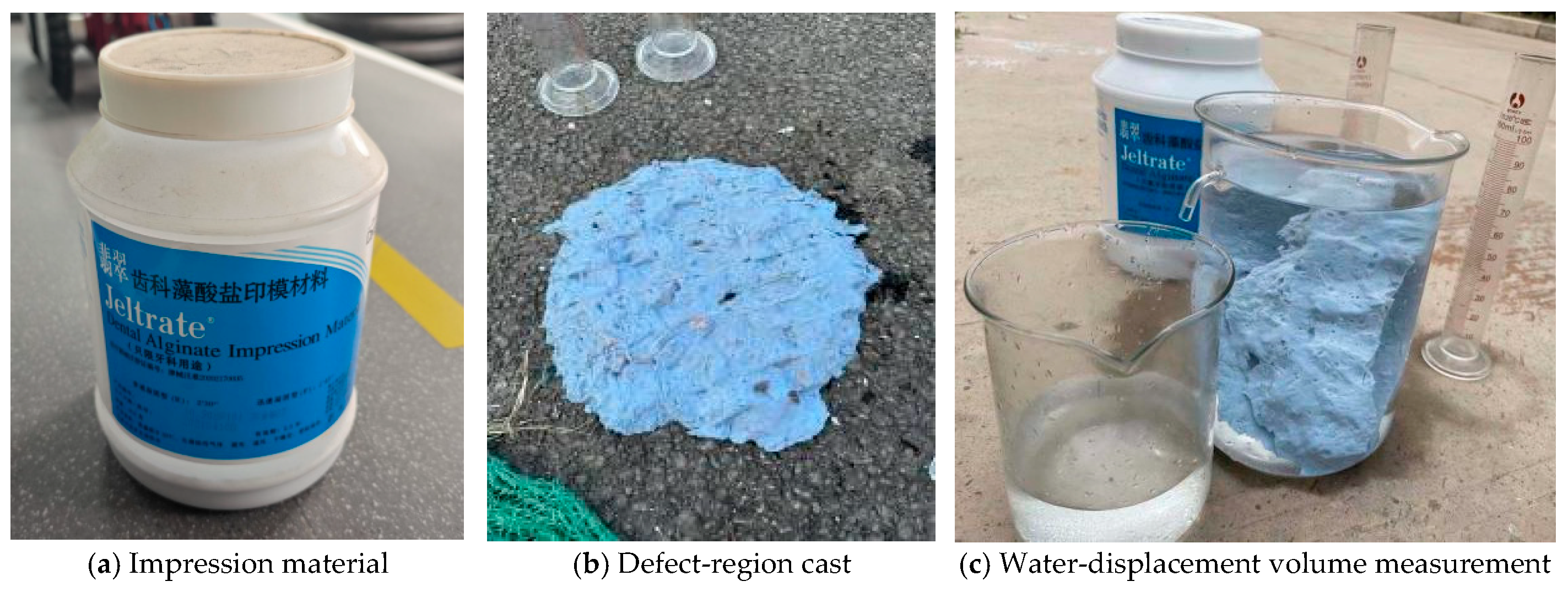
Five independently fabricated specimens were evaluated for each morphology (n = 5 per morphology; n = 15 in total). As shown in Figure 13a–c, alginate impression material was mixed and applied to the defect, smoothed against the curved pipe surface, removed after solidification, and immersed in a measuring cylinder. Each specimen underwent three independent mold-preparation and water-displacement measurements, and their mean was used as the reference volume.

4.2. Comparative Experiments

Poisson Reconstruction [21], conventional Alpha Shape [22], and CAP-UDF [34] were evaluated as reconstruction baselines. The first two represent established implicit and explicit geometric routes, while CAP-UDF provides a contemporary neural implicit comparison.

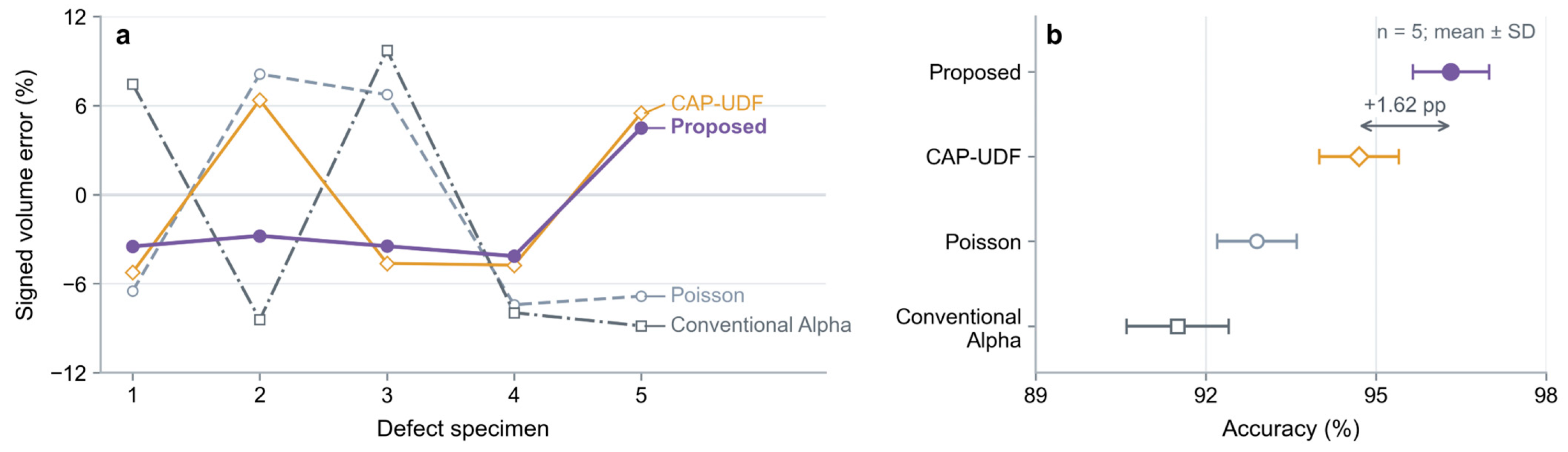
All reconstruction methods used the same defect point clouds obtained from PointNeXt segmentation predictions after the automatic statistical and normal-/curvature-based refinement described in Section 3.3; no manual correction was applied. Reference-surface closure and mesh-volume integration were identical across methods. Therefore, the differences reported in

Table 4. Relative error analysis of circular defects in drainage pipes.

Methodology	Metric	Sample 1	Sample 2	Sample 3	Sample 4	Sample 5	Mean ± SD
Water Displacement	True Volume (cm3)	461.6	803.8	763	1193.2	1557.8	955.9
Poisson Reconstruction	Calculated Volume (cm3)	431.6	869.1	814.4	1104.7	1451.2	934.2
	Accuracy (%)	93.5	91.9	93.3	92.6	93.2	92.9 ± 0.7
	Error (%)	6.5	8.1	6.7	7.4	6.8	7.1 ± 0.7
Conventional Alpha Shape	Calculated Volume (cm3)	496.0	736.1	837.3	1098.3	1420.1	917.6
	Accuracy (%)	92.5	91.6	90.3	92.1	91.2	91.5 ± 0.9
	Error (%)	7.5	8.4	9.7	8.0	8.8	8.5 ± 0.9
CAP-UDF	Calculated Volume (cm3)	437.4	855.1	727.7	1136.5	1643.5	960.0
	Accuracy (%)	94.76	93.62	95.37	95.25	94.50	94.70 ± 0.70
	Error (%)	5.24	6.38	4.63	4.75	5.50	5.30 ± 0.70
Proposed Method	Calculated Volume (cm3)	445.5	781.5	736.5	1143.8	1628.0	947.1
	Accuracy (%)	96.5	97.2	96.5	95.9	95.5	96.3 ± 0.7
	Error (%)	3.5	2.8	3.5	4.1	4.5	3.7 ± 0.7

Note: Each morphology contains n = 5 independently fabricated physical defect specimens. Each specimen was measured three times by water displacement; the reported reference volume is the mean of those repetitions. Mean ± SD summarizes the five independent specimens.

,

Table 5. Relative error analysis of triangular defects in drainage pipes.

Methodology	Metric	Sample 1	Sample 2	Sample 3	Sample 4	Sample 5	Mean ± SD
Water Displacement	True Volume (cm3)	398.6	658.2	542.9	754.3	846.4	640.1
Poisson Reconstruction	Calculated Volume (cm3)	426.4	609.3	579.7	699.0	918.0	646.5
	Accuracy (%)	93.0	92.6	93.2	92.7	91.5	92.6 ± 0.7
	Error (%)	7.0	7.4	6.8	7.3	8.5	7.4 ± 0.7
Conventional Alpha Shape	Calculated Volume (cm3)	362.0	590.8	499.8	820.3	919.7	638.5
	Accuracy (%)	90.8	89.8	92.1	91.2	91.3	91.0 ± 0.8
	Error (%)	9.2	10.2	7.9	8.8	8.7	9.0 ± 0.8
CAP-UDF	Calculated Volume (cm3)	425.0	621.9	514.7	802.6	797.5	632.3
	Accuracy (%)	93.38	94.48	94.81	93.60	94.22	94.10 ± 0.60
	Error (%)	6.62	5.52	5.19	6.40	5.78	5.90 ± 0.60
Proposed Method	Calculated Volume (cm3)	385.7	685.0	528.9	728.2	823.2	630.2
	Accuracy (%)	96.8	95.9	97.4	96.5	97.3	96.8 ± 0.6
	Error (%)	3.2	4.1	2.6	3.5	2.7	3.2 ± 0.6

Note: Each morphology contains n = 5 independently fabricated physical defect specimens. Each specimen was measured three times by water displacement; the reported reference volume is the mean of those repetitions. Mean ± SD summarizes the five independent specimens.

,

Table 6. Relative error analysis of rectangular defects in drainage pipes.

Methodology	Metric	Sample 1	Sample 2	Sample 3	Sample 4	Sample 5	Mean ± SD
Water Displacement	True Volume (cm3)	249.3	526.8	897.5	1368.4	1686	945.6
Poisson Reconstruction	Calculated Volume (cm3)	230.8	569.7	831.7	1276.3	1824.9	946.7
	Accuracy (%)	92.6	91.9	92.7	93.3	91.8	92.4 ± 0.6
	Error (%)	7.5	8.1	7.3	6.7	8.2	7.6 ± 0.6
Conventional Alpha Shape	Calculated Volume (cm3)	273.7	481.4	979.7	1507.9	1540.8	956.7
	Accuracy (%)	90.2	91.4	90.9	89.8	91.4	90.7 ± 0.7
	Error (%)	9.8	8.6	9.2	10.2	8.6	9.3 ± 0.7
CAP-UDF	Calculated Volume (cm3)	266.6	497.6	951.1	1463.6	1591.7	954.1
	Accuracy (%)	93.06	94.46	94.03	93.04	94.41	93.80 ± 0.70
	Error (%)	6.94	5.54	5.97	6.96	5.59	6.20 ± 0.70
Proposed Method	Calculated Volume (cm3)	242.4	510.1	865.1	1406.6	1629.0	930.6
	Accuracy (%)	97.2	96.8	96.4	97.2	96.6	96.9 ± 0.4
	Error (%)	2.8	3.2	3.6	2.8	3.4	3.2 ± 0.4

Note: Each morphology contains n = 5 independently fabricated physical defect specimens. Each specimen was measured three times by water displacement; the reported reference volume is the mean of those repetitions. Mean ± SD summarizes the five independent specimens.

,

Table 7. Paired-bootstrap analysis of volumetric error reduction.

Morphology	Conventional Error (%)	Proposed Error (%)	Reduction (pp)	95% Bootstrap CI (pp)
Circular	8.48	3.68	4.80	[3.98, 5.68]
Triangular	8.95	3.22	5.74	[5.43, 6.03]
Rectangular	9.27	3.14	6.13	[5.38, 6.94]
Overall	8.90	3.35	5.56	[5.17, 5.97]

Note: For the overall estimate, paired differences were resampled within each morphology, and the three morphology-level means were averaged in each bootstrap replicate.

and

Table 8. Volume-accuracy sensitivity to the RANSAC inlier threshold.

Threshold	Circular (%)	Triangular (%)	Rectangular (%)	Overall (%)
2.0 mm	96.54 ± 0.67	97.00 ± 0.60	97.07 ± 0.36	96.87 ± 0.57
2.5 mm	96.32 ± 0.67	96.78 ± 0.60	96.86 ± 0.37	96.65 ± 0.57
3.0 mm	95.79 ± 0.67	96.24 ± 0.60	96.32 ± 0.37	96.12 ± 0.57

and Figure 14, Figure 15 and Figure 16 reflect the reconstruction method.

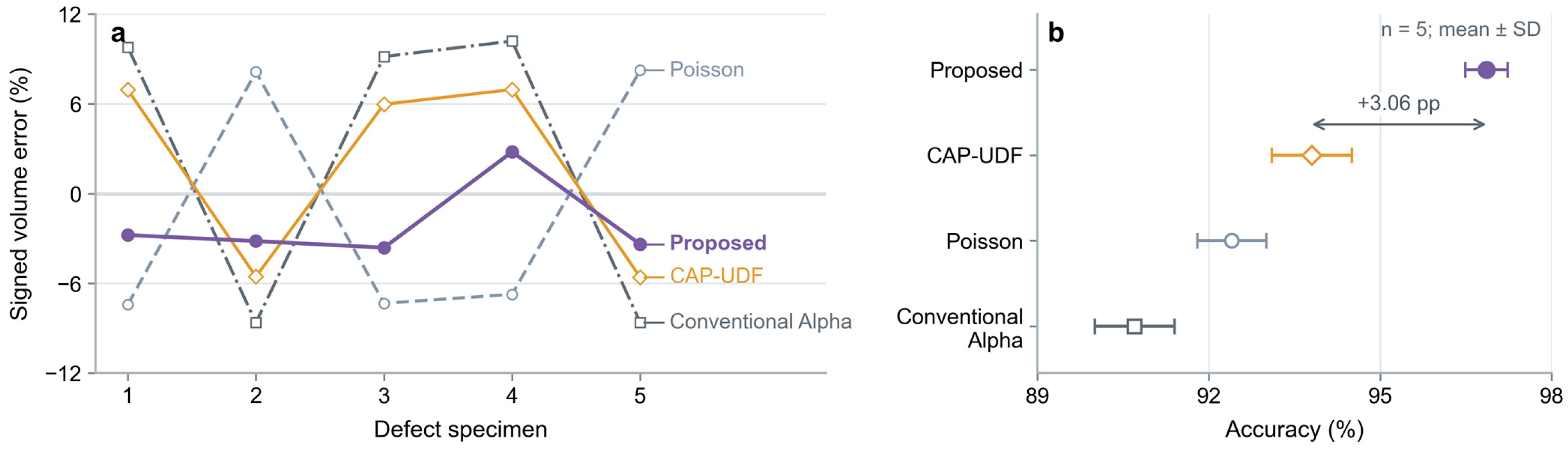
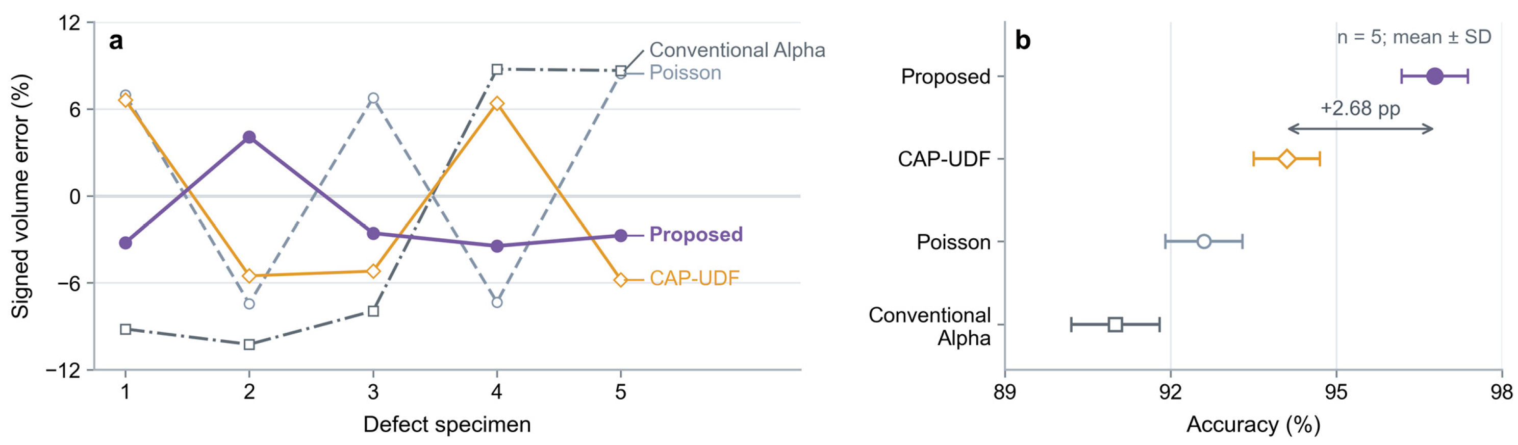
Table 4, Table 5 and Table 6 report specimen-level results under this common protocol. The proposed density-adaptive Alpha Shape method achieved mean volume accuracies of 96.32%, 96.78%, and 96.86% for circular, triangular, and rectangular defects, respectively, compared with 94.70%, 94.10%, and 93.80% for CAP-UDF. This corresponds to improvements of 1.62, 2.68, and 3.06 percentage points over CAP-UDF, respectively.

The paired-bootstrap analysis of volumetric error reduction is summarized in Table 7. Paired-bootstrap resampling estimated error reductions of 4.80, 5.74, and 6.13 percentage points for circular, triangular, and rectangular defects, respectively. The overall reduction was 5.56 percentage points (95% CI: [5.17, 5.97]), with the interval remaining above zero.

The nominal RANSAC inlier threshold of 2.5 mm was varied by ±20% while the downstream density-adaptive reconstruction and volume-integration procedure was held constant.The corresponding sensitivity results are summarized in Table 8.

Across the tested range, overall volume accuracy varied from 96.12% to 96.87%, corresponding to a 0.75-percentage-point span and indicating limited sensitivity to moderate changes in the RANSAC inlier threshold.

5. Discussion

Under controlled laboratory conditions, local-density adaptation improved surface continuity and volume accuracy over fixed-parameter reconstruction, while water-displacement references provided direct physical calibration of the reconstructed volumes.

5.1. Validity of Laboratory Datasets and Real-World Generalization

The controlled laboratory platform provided repeatable physical volume references and isolated the geometric reconstruction question. Operational drainage pipelines introduce a distinct sensing domain: wet or reflective surfaces can produce ToF multipath and specular-reflection errors, while biological scaling, sediment, and residual moisture can obscure defect boundaries or generate spatially correlated outliers. The current statistical and normal-/curvature-based refinement targets isolated geometric noise; field validation should therefore focus on these non-Gaussian disturbances. Within the controlled domain, synthetic augmentation improved performance on the held-out real test set.

5.2. Applicability to Dynamic Robotic Inspection Systems

The reconstruction framework can accept spatially registered point clouds from a mobile platform, but deployment introduces robot motion, sensor vibration, occlusion, water interference, lighting variation, and registration drift beyond the static acquisition conditions evaluated here. Mobile integration therefore depends on a dedicated acquisition-and-registration validation stage. Once reliable registered point clouds are available, the proposed geometry and volume modules can be evaluated without changing their core reconstruction logic.

5.3. Scope of Defect Analysis: Structural Defects Versus Functional Anomalies

This study focuses on negative defects (concave surface anomalies), such as spalling, corrosion, and cavities, which correspond to material loss and directly compromise the structural integrity of concrete pipelines. Positive defects, including root intrusion and sediment deposition, were not considered in the volumetric experiments.

The fitted cylindrical wall provides the geometric reference for distinguishing inward material-loss defects from outward protrusions. The present experiments and quantitative claims concern material loss; extending the measurement protocol to root intrusion or sediment deposition requires category-specific validation and reference measurements.

5.4. Applicability to Irregular Defect Geometries

Regular-shaped defects (circular, triangular, rectangular) were adopted in the experiments to enable accurate theoretical volume calculation and dual validation with the water displacement method. This design enables direct error quantification under controlled conditions.

The density-adaptive method is driven by local spacing rather than a predefined defect shape. Equations (9) and (10) assign smaller reconstruction scales to dense boundary regions and larger scales to sparse regions. Across the three tested boundary geometries, the proposed method maintained higher volume accuracy than the compared reconstruction baselines.

5.5. Hydraulic Implications of Quantified Defect Geometry

The reconstructed surfaces provide geometric inputs for subsequent hydraulic assessment. Local material-loss cavities alter the cross-section and wetted surface, which can promote flow separation, recirculation, and additional energy loss. At a larger spatial scale, accumulated deterioration can contribute to changes in equivalent roughness used in one-dimensional sewer models and can influence sediment-transport conditions [35,36]. The present volume metric is a geometric quantity rather than a direct estimate of hydraulic loss or Manning roughness. Quantitative hydraulic relationships can be established by coupling the reconstructed geometries with CFD simulations or controlled hydraulic experiments.

6. Conclusions

This study developed an integrated point-cloud framework for the three-dimensional reconstruction and volume quantification of concrete drainage pipeline defects. The framework connects WCPC-GAN-based data augmentation, PointNeXt semantic segmentation, geometry-constrained point-cloud refinement, density-adaptive surface reconstruction, and physical volume validation.

WCPC-GAN incorporates a local warping mechanism into a relatively lightweight generative architecture to improve the representation of local defect geometry and provide additional labeled point clouds for model development. For quantitative reconstruction, RANSAC-based cylindrical fitting and Delaunay triangulation are combined with a density-adaptive Alpha Shape strategy. By adjusting the reconstruction parameter according to local point-cloud density, the method improves boundary preservation and surface continuity while reducing holes and other topological artifacts associated with fixed-parameter reconstruction.

Using PointNeXt-derived point clouds without manual correction, the complete automatic pipeline achieved mean volume accuracies of 96.32 ± 0.67%, 96.78 ± 0.60%, and 96.86 ± 0.37% for circular, triangular, and rectangular defects. The proposed reconstruction retained the highest mean accuracy across conventional Alpha Shape, Poisson, and CAP-UDF baselines. Paired-bootstrap analysis estimated an overall 5.56-percentage-point error reduction over conventional Alpha Shape (95% CI: 5.17–5.97). Local density adaptation preserved the highest accuracy across all three tested morphologies while remaining stable to moderate RANSAC-threshold changes.

Future work will evaluate the framework using operational-pipeline point clouds affected by mobile registration, wet-surface ToF interference, occlusion, and field-specific noise, and will further couple the reconstructed geometries with CFD or controlled hydraulic experiments.

References

1. American Society of Civil Engineers. 2017 Infrastructure Report Card; American Society of Civil Engineers: Reston, VA, USA, 2017; Available online: https://2017.infrastructurereportcard.org/ (accessed on 19 August 2026).
2. Hawari, A.; Alkadour, F.; Elmasry, M.; Zayed, T. A state of the art review on condition assessment models developed for sewer pipelines. Eng. Appl. Artif. Intell. 2020, 93, 103721. [Google Scholar] [CrossRef] [Scilit]
3. Mugume, S.N.; Gomez, D.E.; Fu, G.; Farmani, R.; Butler, D. A global analysis approach for investigating structural resilience in urban drainage systems. Water Res. 2015, 81, 15–26. [Google Scholar] [CrossRef] [Scilit] [PubMed]
4. Haurum, J.B.; Moeslund, T.B. A survey on image-based automation of CCTV and SSET sewer inspections. Autom. Constr. 2020, 111, 103061. [Google Scholar] [CrossRef] [Scilit]
5. Foorginezhad, S.; Mohseni-Daragh, M.; Firoozirad, K.; Aryai, V.; Razmjou, A.; Abbassi, R.; Garaniya, V.; Beheshti, A.; Asadnia, M. Recent advances in sensing and assessment of corrosion in sewage pipelines. Process Saf. Environ. Prot. 2021, 147, 192–213. [Google Scholar] [CrossRef] [Scilit]
6. Anbari, M.J.; Tabesh, M.; Roozbahani, A. Risk assessment model to prioritize sewer pipes inspection in wastewater collection networks. J. Environ. Manag. 2017, 190, 91–101. [Google Scholar] [CrossRef] [Scilit] [PubMed]
7. Jahanshahi, M.R.; Masri, S.F. A new methodology for non-contact accurate crack width measurement through photogrammetry for automated structural safety evaluation. Smart Mater. Struct. 2013, 22, 035019. [Google Scholar] [CrossRef] [Scilit]
8. Guo, Y.; Wang, H.; Hu, Q.; Liu, H.; Liu, L.; Bennamoun, M. Deep learning for 3D point clouds: A survey. IEEE Trans. Pattern Anal. Mach. Intell. 2021, 43, 4338–4364. [Google Scholar] [CrossRef] [Scilit] [PubMed]
9. Xie, Y.; Tian, J.; Zhu, X.X. Linking points with labels in 3D: A review of point cloud semantic segmentation. IEEE Geosci. Remote Sens. Mag. 2020, 8, 38–59. [Google Scholar] [CrossRef] [Scilit]
10. Qi, C.R.; Yi, L.; Su, H.; Guibas, L.J. PointNet++: Deep hierarchical feature learning on point sets in a metric space. In Advances in Neural Information Processing Systems 30; Guyon, I., von Luxburg, U., Bengio, S., Wallach, H., Fergus, R., Vishwanathan, S., Garnett, R., Eds.; Curran Associates, Inc.: Red Hook, NY, USA, 2017; pp. 5099–5108. [Google Scholar]
11. Wang, Y.; Sun, Y.; Liu, Z.; Sarma, S.E.; Bronstein, M.M.; Solomon, J.M. Dynamic graph CNN for learning on point clouds. ACM Trans. Graph. 2019, 38, 146. [Google Scholar] [CrossRef] [Scilit]
12. Zhang, J.; Zhou, Z.; Sun, J. Three-dimensional segmentation and global clearance analysis for free-bent pipelines in point-cloud scenarios. IEEE Trans. Instrum. Meas. 2023, 72, 2511712. [Google Scholar] [CrossRef] [Scilit]
13. Cui, X.; Li, Y.; Li, J.; Zhang, J. Cross-PIC: A cross-scale in-context learning network for 3D multibeam point cloud segmentation of submarine pipelines. Ocean Eng. 2025, 315, 119778. [Google Scholar] [CrossRef] [Scilit]
14. Wang, N.; Ma, D.; Du, X.; Li, B.; Di, D.; Pang, G.; Duan, Y. An automatic defect classification and segmentation method on three-dimensional point clouds for sewer pipes. Tunn. Undergr. Space Technol. 2024, 143, 105480. [Google Scholar] [CrossRef] [Scilit]
15. Pang, G.; Wang, N.; Fang, H.; Liu, H.; Huang, F. Study of damage quantification of concrete drainage pipes based on point cloud segmentation and reconstruction. Buildings 2022, 12, 213. [Google Scholar] [CrossRef] [Scilit]
16. Yang, X.; Wu, Y.; Zhang, K.; Jin, C. CPCGAN: A controllable 3D point cloud generative adversarial network with semantic label generating. Proc. AAAI Conf. Artif. Intell. 2021, 35, 3154–3162. [Google Scholar] [CrossRef] [Scilit]
17. Tang, Y.; Qian, Y.; Zhang, Q.; Zeng, Y.; Hou, J.; Zhe, X. WarpingGAN: Warping multiple uniform priors for adversarial 3D point cloud generation. In Proceedings of the IEEE/CVF Conference on Computer Vision and Pattern Recognition, New Orleans, LA, USA, 18–24 June 2022; pp. 6387–6395. [Google Scholar] [CrossRef] [Scilit]
18. Liu, Y.; Yang, M.; Jiang, P. CGAN-driven intelligent generative design of vehicle exterior shape. Expert Syst. Appl. 2025, 274, 127066. [Google Scholar] [CrossRef] [Scilit]
19. Liu, L.; Cao, D.; Wu, Y.; Wei, T. Defective samples simulation through adversarial training for automatic surface inspection. Neurocomputing 2019, 360, 230–245. [Google Scholar] [CrossRef] [Scilit]
20. Bang, H.; Min, J.; Jeon, H. Deep learning-based concrete surface damage monitoring method using structured lights and depth camera. Sensors 2021, 21, 2759. [Google Scholar] [CrossRef] [Scilit] [PubMed]
21. Kazhdan, M.; Bolitho, M.; Hoppe, H. Poisson surface reconstruction. In Proceedings of the Fourth Eurographics Symposium on Geometry Processing, Cagliari, Italy, 26–28 June 2006; Sheffer, A., Polthier, K., Eds.; Eurographics Association: Goslar, Germany, 2006; pp. 61–70. [Google Scholar] [CrossRef]
22. Edelsbrunner, H.; Mücke, E.P. Three-dimensional alpha shapes. ACM Trans. Graph. 1994, 13, 43–72. [Google Scholar] [CrossRef] [Scilit]
23. Yin, C.; Cheng, J.C.P.; Wang, B.; Gan, V.J.L. Automated classification of piping components from 3D LiDAR point clouds using SE-PseudoGrid. Autom. Constr. 2022, 139, 104300. [Google Scholar] [CrossRef] [Scilit]
24. Arjovsky, M.; Chintala, S.; Bottou, L. Wasserstein GAN. In Proceedings of the 34th International Conference on Machine Learning, Sydney, Australia, 6–11 August 2017; Precup, D., Teh, Y.W., Eds.; Proceedings of Machine Learning Research; PMLR: New York, NY, USA, 2017; Volume 70, pp. 214–223. [Google Scholar]
25. Gulrajani, I.; Ahmed, F.; Arjovsky, M.; Dumoulin, V.; Courville, A.C. Improved training of Wasserstein GANs. In Advances in Neural Information Processing Systems 30; Curran Associates, Inc.: Red Hook, NY, USA, 2017; pp. 5767–5777. [Google Scholar]
26. Schnabel, R.; Wahl, R.; Klein, R. Efficient RANSAC for point-cloud shape detection. Comput. Graph. Forum 2007, 26, 214–226. [Google Scholar] [CrossRef] [Scilit]
27. Lee, D.T.; Schachter, B.J. Two algorithms for constructing a Delaunay triangulation. Int. J. Comput. Inf. Sci. 1980, 9, 219–242. [Google Scholar] [CrossRef] [Scilit]
28. Zhou, K.; Hou, Q.; Wang, R.; Guo, B. Real-time KD-tree construction on graphics hardware. ACM Trans. Graph. 2008, 27, 126. [Google Scholar] [CrossRef] [Scilit]
29. Shu, D.W.; Park, S.W.; Kwon, J. 3D point cloud generative adversarial network based on tree structured graph convolutions. In Proceedings of the IEEE/CVF International Conference on Computer Vision, Seoul, Republic of Korea, 27 October–2 November 2019; pp. 3859–3868. [Google Scholar] [CrossRef] [Scilit]
30. Qian, G.; Li, Y.; Peng, H.; Mai, J.; Hammoud, H.A.A.K.; Elhoseiny, M.; Ghanem, B. PointNeXt: Revisiting PointNet++ with improved training and scaling strategies. In Advances in Neural Information Processing Systems 35; Curran Associates, Inc.: Red Hook, NY, USA, 2022; pp. 23192–23204. [Google Scholar]
31. Potter, J.E.; Stern, R.G. Statistical filtering of space navigation measurements. In Proceedings of the AIAA Guidance and Control Conference, Cambridge, MA, USA, 12–14 August 1963. AIAA Paper 63-333. [Google Scholar] [CrossRef] [Scilit]
32. Abdi, H.; Williams, L.J. Principal component analysis. Wiley Interdiscip. Rev. Comput. Stat. 2010, 2, 433–459. [Google Scholar] [CrossRef] [Scilit]
33. Mérigot, Q.; Ovsjanikov, M.; Guibas, L.J. Voronoi-based curvature and feature estimation from point clouds. IEEE Trans. Vis. Comput. Graph. 2011, 17, 743–756. [Google Scholar] [CrossRef] [Scilit] [PubMed]
34. Zhou, J.; Ma, B.; Li, S.; Liu, Y.-S.; Fang, Y.; Han, Z. CAP-UDF: Learning unsigned distance functions progressively from raw point clouds with consistency-aware field optimization. IEEE Trans. Pattern Anal. Mach. Intell. 2024, 46, 7475–7492. [Google Scholar] [CrossRef] [Scilit] [PubMed]
35. Banasiak, R. Hydraulic performance of sewer pipes with deposited sediments. Water Sci. Technol. 2008, 57, 1743–1748. [Google Scholar] [CrossRef] [Scilit] [PubMed]
36. Coelho, F.M.; de Azevedo, J.P.S. Design criteria for roughness values under real sewer system operating conditions. J. Pipeline Syst. Eng. Pract. 2022, 13, 04022018. [Google Scholar] [CrossRef] [Scilit]
Figure 1. Overall workflow of the proposed point-cloud-based framework for drainage pipeline defect reconstruction and volume quantification.
Infrastructures 11 00300 g001
Figure 2. CPCGAN network architecture. In the figure, “*” is retained as a tensor-dimension separator (e.g., 3296 and 2048*3), while “x” in 32x and 64x denotes the expansion or repetition factor rather than a multiplication sign. Arrows indicate the direction of data flow, the ellipsis (…) represents repeated MLP branches, and “+” denotes the addition operation. Blue-toned elements represent the structural point-cloud pathway, whereas green-toned elements represent the complete point-cloud pathway. The upper and lower background regions correspond to the generator and discriminator components, respectively, and the dashed outlines delimit the Structural Generative Network and Final Generative Network.
Infrastructures 11 00300 g002
Figure 3. Architecture of the local-warping module. Global encoding and local feature encoding are fused with the predefined prior point cloud and subsequently processed by MLP layers to generate the concatenated feature output. Arrows indicate the direction of data flow. Yellow elements denote global-feature encoding and feature-fusion operations, blue denotes local-feature encoding, gray denotes the predefined prior point cloud, and green denotes the MLP processing and output stages.
Infrastructures 11 00300 g003
Figure 4. Network architecture of the WCPC-GAN auxiliary generator. Features from the primary generator are processed through the self-attention and local-warping branches before being fused to produce the auxiliary-generator output. In the figure, “*” is retained as a tensor-dimension separator (e.g., 3296 and 2048*3), while “x” in 64x denotes the expansion or repetition factor rather than a multiplication sign. Arrows indicate the direction of data flow, “+” denotes feature addition, and the ellipsis (…) indicates repeated parallel MLP branches where applicable. Different colors distinguish the primary-generator input, feature-processing branches, expansion operations, and fused output.
Infrastructures 11 00300 g004
Figure 5. Schematic of a spatial cylinder.
Infrastructures 11 00300 g005
Figure 6. Schematic of three-dimensional Delaunay triangulation. Red points represent the sampled vertices, gray lines denote the Delaunay edges connecting neighboring vertices, and the cyan triangular face illustrates a representative triangular facet of the constructed mesh.
Infrastructures 11 00300 g006
Figure 7. Surface reconstruction results for defective regions.
Infrastructures 11 00300 g007
Figure 8. Real data of pipeline defects: (a) representative rectangular defects; (b) representative circular defects; (c) representative triangular defects; (d) Microsoft Azure Kinect DK depth camera used for point-cloud acquisition.
Infrastructures 11 00300 g008
Figure 9. Comparison of point-cloud augmentation results generated by different networks: (a) TreeGAN; (b) CPCGAN; (c) WarpingGAN; (d) WCPC-GAN.
Infrastructures 11 00300 g009
Figure 10. Representative defect point clouds augmented by WCPC-GAN. The color variation is used only for 3D visualization of the generated point-cloud geometry and does not represent different defect classes or quantitative values.
Infrastructures 11 00300 g010
Figure 11. Structure of the PointNeXt model. Yellow/orange blocks denote MLP and set-abstraction operations, gray-blue blocks denote inverted residual MLP (InvResMLP) modules, and blue blocks denote feature-propagation stages. Arrows indicate the direction of feature flow, while the long connecting lines represent multiscale skip connections between the encoder and decoder stages.
Infrastructures 11 00300 g011
Figure 12. Comparison of point clouds before and after statistical filtering: (a) point cloud before statistical filtering; (b) point cloud after statistical filtering.The white contour indicating the region containing prominent outliers targeted by the filtering procedure.
Infrastructures 11 00300 g012
Figure 13. Water-displacement reference measurement: (a) commercially available alginate impression material; (b) solidified defect-region cast; (c) water-displacement volume reading in a measuring cylinder.
Infrastructures 11 00300 g013
Figure 14. Volumetric comparison for circular defects: (a) signed volume error of the four reconstruction methods across five independently fabricated specimens; (b) mean volume accuracy (mean ± SD) of the four reconstruction methods. Different colors, line styles, and markers distinguish the reconstruction methods, as identified by the labels in each panel.
Infrastructures 11 00300 g014
Figure 15. Volumetric comparison for triangular defects: (a) signed volume error of the four reconstruction methods across five independently fabricated specimens; (b) mean volume accuracy (mean ± SD) of the four reconstruction methods. Different colors, line styles, and markers distinguish the reconstruction methods, as identified by the labels in each panel.
Infrastructures 11 00300 g015
Figure 16. Volumetric comparison for rectangular defects: (a) signed volume error of the four reconstruction methods across five independently fabricated specimens; (b) mean volume accuracy (mean ± SD) of the four reconstruction methods. Different colors, line styles, and markers distinguish the reconstruction methods, as identified by the labels in each panel.
Infrastructures 11 00300 g016