Reliability-Based Slope Stability Analysis Using Particle Swarm-Optimized Neural Network: Benchmarking Against Conventional Probabilistic Methods Using a Lebanese Case Study

Abstract

Probabilistic slope stability analysis requires tools that are both computationally efficient and accurate for uncertainty propagation. This study develops a reliability-oriented surrogate framework coupling a multilayer perceptron artificial neural network with particle swarm optimization (ANN–MLP–PSO). The model was trained on 2014 homogeneous slope cases drawn from literature records and mechanics-based simulations. PSO identified a best-performing six-hidden-layer architecture achieving a coefficient of determination of R² = 0.95 on the held-out test set. The trained surrogate was embedded in a probabilistic sampling framework to estimate the probability of failure (P_f), reliability index (β), and factor-of-safety quantiles, then applied to the Mansourieh slope near Beirut, Lebanon, under dry and wet conditions. Outputs were benchmarked against the First-Order Second-Moment method (FOSM), the Point Estimate Method (PEM), and Monte Carlo simulation (MCS). The comparison showed that the ANN–MLP–PSO surrogate reproduced the dry-to-wet changes in factor-of-safety distributions, probability of failure, and reliability index obtained from the conventional reliability methods under the same probabilistic assumptions, with wet-scenario failure probabilities ranging from approximately 86% to 99%. Despite quantitative differences, all four methods identified the same reliability trend and engineering interpretation. Once trained, the surrogate enabled rapid probabilistic evaluation without repeated deterministic calculations, providing an efficient tool for slope stability screening and uncertainty-aware geotechnical decision support.

1. Introduction

Slope stability is a central concern in geotechnical engineering. Failures of natural or engineered slopes may lead to severe human, economic, and environmental consequences, particularly in earth dams, embankments, excavations, and landfills [1,2]. In practice, stability is commonly evaluated through a factor of safety (FoS) computed using Limit Equilibrium Methods (LEM) and, in other settings, Finite Element Methods (FEM) [3]. However, the FoS is a single deterministic index that does not explicitly represent the substantial uncertainties in soil properties [4,5,6,7], geometry, loading, and modeling assumptions. This can lead to either unconservative or overly conservative designs when variability matters. Recent geotechnical and reliability literature emphasizes this limitation while reaffirming LEM/FEM as the baseline for professional practice [8,9,10,11]. For slopes where pore-pressure fluctuations and soil variability control performance, a single deterministic FoS can hide important risk information [12,13].

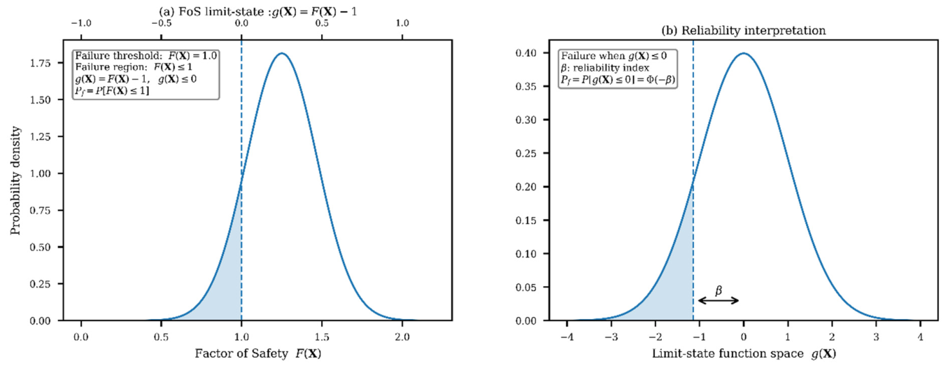
Landslides represent a recurrent geohazard in Lebanon, where steep topography and road cuts intersect with intense winter storms, making rainfall-triggered instabilities a practical concern for infrastructure safety. Flooding and heavy rainfall episodes are also reported to contribute to landslide triggering, reinforcing the need to treat pore-pressure conditions probabilistically when evaluating slope performance. Therefore, the present study adopts a Lebanese field case (the Mansourieh slope) and explicitly examines the dry-to-wet reliability shift driven by pore-pressure uncertainty. To explicitly incorporate uncertainty, probabilistic reliability methods complement conventional mechanics by propagating distributions of input parameters through the stability calculation to obtain outputs such as probability of failure (P_f) and reliability index (β) [14,15,16]. The First-Order Second-Moment method (FOSM) estimates reliability through a first-order approximation based on the moments of the input variables, whereas the First-Order Reliability Method (FORM) evaluates the limit-state function at a design point in transformed probability space. The Second-Order Reliability Method (SORM) extends FORM by incorporating the local curvature of the limit-state surface, which can improve reliability estimations for nonlinear response functions, although it requires additional design-point and curvature calculations [17,18,19,20,21,22]. More recently, the quantile-based first-order second-moment method (QFOSM) has been introduced as an efficient alternative that retains computational simplicity comparable to conventional FOSM while providing reliability estimates approaching FORM accuracy without requiring the iterative optimization normally associated with FORM. QFOSM has also been extended to slope reliability and parameter-sensitivity analysis, demonstrating its relevance to probabilistic slope stability assessment [23,24]. In the present study, FOSM, PEM, and MCS were retained as representative moment-based, point-estimate, and sampling-based benchmark approaches, respectively, while QFOSM and SORM are recognized as relevant alternative reliability methods beyond the selected benchmarking scope.

Point-Estimate Methods (PEM), originally proposed by Rosenblueth [25,26], replace probability distributions with weighted discrete realizations and provide efficient approximations of moments and reliability measures with few structured evaluations [25,26,27,28,29,30,31,32,33]; Monte Carlo simulation (MCS) remains among the most widely adopted techniques due to its conceptual simplicity and robustness, though it is computationally demanding. In slope stability, MCS involves repeated sampling of uncertain soil and geometric variables (e.g., cohesion, friction angle, unit weight), the computation of FoS for each realization, and estimation of β and Pf from the resulting response distribution [21,34,35,36,37]. These approaches support risk-informed decisions through probabilistic tools that offer rigorous reliability estimation. However, their computational burden is often a major obstacle in practical engineering contexts, particularly when repeated analyses are required.

Parallel to the growth of reliability methods, machine learning (ML) [1,5,38,39,40,41,42,43,44] and in particular artificial neural networks (ANNs) [45,46,47,48,49] have been widely explored to model complex, nonlinear relationships between geotechnical inputs and slope stability responses [46,50,51,52,53,54]. Numerous studies and recent reviews report that data-driven models can achieve high predictive accuracy and speed, with growing use as surrogates or complements to physics-based analyses. The literature highlights challenges such as limited or synthetic datasets, overfitting risks, and the need to align ML outputs with geotechnical interpretability and uncertainty considerations. ANN-based models have been widely applied to predict FoS in slope stability and have shown strong nonlinear mapping capability across a range of input descriptions. However, reported performance is often sensitive to dataset representativeness and training configuration, and many studies rely on limited or simulation-driven datasets, motivating the use of robust optimization and more rigorous validation under uncertainty [55,56,57]. Sakellariou and Ferentinou [58] compared ANN predictions of FoS with classical analytical methods, while Das et al. [59] developed ANN models using key geotechnical and geometric parameters (e.g., slope height, unit weight, cohesion, friction angle, slope gradient, and pore pressure), reporting close agreement with field-referenced outcomes. Choobbasti et al. [60] incorporated total and effective stress conditions, slope geometry, shear strength parameters, and seismic coefficients, concluding that ANN outputs provide a strong approximation to Bishop’s method. Samui and Kothari [61] introduced a least-square support vector machine (LSSVM) and compared it with ANN, showing superior predictive accuracy for LSSVM under their tested conditions. Erzin and Cetin [62] further demonstrated ANN capability by training models on 675 Bishop-based cases, reporting improved performance relative to multiple regression, particularly when broader input descriptions were included.

Particle Swarm Optimization (PSO), originally introduced by Kennedy and Eberhart [63], is a population-based metaheuristic inspired by collective behavioral patterns observed in bird flocking and fish schooling. In PSO, candidate solutions (particles) iteratively adjust their trajectories within the search space by learning from both individual experience and the best-performing solution within the population [64,65,66,67]. Owing to its simplicity, computational efficiency, and balance between local exploitation and global exploration, PSO has been widely adopted across engineering optimization problems. In the context of slope stability, PSO has been applied both as a direct optimizer and as a hybrid tool to enhance ANN predictive performance. Kalatehjari et al. [68] applied PSO to identify critical slip surfaces in homogeneous slopes using Bishop’s method, demonstrating strong global search efficiency without incorporating data-driven learning. More recent studies combined PSO and ANN to predict slope stability; however, several limitations persist. Rukhaiyar et al. [69] developed a PSO–ANN model using only 83 cases and adopting a fixed network architecture, while Gordan et al. [70] relied on synthetic datasets generated via GeoStudio, which may restrict generalizability. Similarly, Moayedi et al. [71] developed ANN, ANFIS, and PSO–ANN models based on FEM-generated datasets and reported near-perfect predictive coefficients, yet such performance may reflect overfitting behavior arising from simulation-driven datasets that do not fully represent real field variability. In contrast, Li et al. [66] applied a PSO–MLP framework to landslide susceptibility mapping in Jiangxi Province, China using 369 real landslide cases, where PSO was employed to tune hyperparameters such as learning rate, momentum, and hidden neuron configuration. Their results demonstrated improved predictive capability compared to benchmark models, highlighting the potential of PSO-enhanced neural frameworks in geotechnical risk applications. Additional integrations include Luo et al. [72], who coupled PSO with the Cubist Algorithm for slope safety prediction, and Chen et al. [73], who embedded PSO within three-dimensional reliability frameworks to search for ellipsoidal slip surfaces under spatial variability. Overall, existing studies confirm PSO’s usefulness both for optimization in mechanics-based slope stability tasks and for enhancing machine learning performance. However, many ANN–PSO applications remain constrained by synthetic datasets, limited input parameter ranges, or validations restricted to deterministic comparisons, leaving uncertainty-related benchmarking largely unexplored [54].

Based on the reviewed literature, it has not yet been established whether hybrid ANN–PSO frameworks can reproduce probabilistic reliability outputs (P_f, β, and FoS distribution characteristics) at a level consistent with established approaches such as FOSM, PEM, and MCS, particularly under realistic geotechnical conditions. Most existing ANN–PSO slope stability applications have been limited by synthetic datasets, narrow geotechnical input domains, or benchmarking restricted to deterministic methods. To address these gaps, the present study develops an ANN multilayer perceptron optimized using particle swarm optimization (ANN–MLP–PSO) and trained on a large dataset of homogeneous slope cases, then applies the framework to a documented field case study at the Mansourieh slope near Beirut, Lebanon. The key novelty is the reformulation of ANN–MLP–PSO as a reliability-consistent surrogate, explicitly validated against FOSM, PEM, and MCS under identical limit-state and uncertainty models. The study further demonstrates a dry-to-wet hydraulic reliability transition consistent with the expected influence of increasing pore-water pressure, showing how the pore water pressure ratio (R_u) controls the shift of the FoS distribution into the failure domain. Finally, by replacing repeated Morgenstern–Price evaluations with rapid ANN inference during sampling, the proposed framework delivers substantial computational gains while maintaining agreement with conventional reliability metrics, supporting scalable uncertainty-aware slope assessment for practical geotechnical workflows. This paper makes the following contributions:

• It develops an optimized ANN–MLP–PSO surrogate trained on a large slope dataset covering broad geometrical, strength, and pore-pressure conditions.
• It extends deterministic surrogate prediction to probabilistic post-processing, where sampled inputs are propagated through the trained ANN to compute P_f, β, and FoS quantiles under dry and wet conditions.
• It evaluates the probabilistic behavior of ANN-derived reliability outputs relative to benchmark reliability approaches (FOSM, PEM, and MCS) under consistent probabilistic characterization.

Although ANN–PSO frameworks have previously been applied to deterministic slope stability prediction, their ability to reproduce probabilistic reliability metrics and reliability trends consistent with established methods remains insufficiently investigated. Accordingly, the objective of the present study is to develop and evaluate a reliability-oriented ANN–MLP–PSO surrogate framework capable of estimating probability of failure (Pf), reliability index (β), and factor-of-safety distribution characteristics under uncertainty. The proposed framework is benchmarked against FOSM, PEM, and Monte Carlo simulation under consistent probabilistic assumptions and is demonstrated through application to a representative Lebanese slope case study. The study therefore focuses on extending ANN–PSO methodology from deterministic prediction toward practical reliability-based geotechnical decision support.

2. Methodology

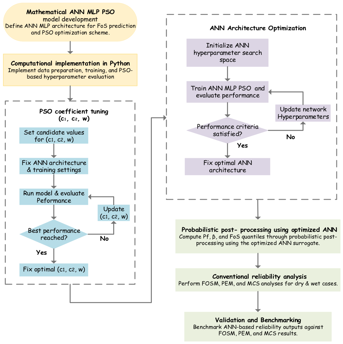
This study follows a staged workflow to develop and validate a reliability-oriented ANN–MLP–PSO framework for slope stability assessment. The procedure begins with formulating the ANN surrogate for FoS prediction and defining the PSO scheme used for hyperparameter optimization. The complete pipeline is then implemented in Python 3.10.11 and used in two sequential optimization steps. First, PSO control coefficients are calibrated through sensitivity analysis. Second, with fixed PSO coefficients, the ANN architecture and key training settings are optimized to obtain a stable high-accuracy surrogate. The optimized ANN is subsequently embedded in a probabilistic sampling procedure to compute reliability indicators, which are finally benchmarked against conventional probabilistic approaches for the Mansourieh slope case study (Lebanon) under both dry and wet conditions. The overall methodology is visualized in Figure 1. It is organized into the following seven stages:

• Stage 1—Formulation: Define the ANN–MLP input–output mapping for FoS and specify the PSO update equations adopted for optimization.
• Stage 2—Implementation: Implement the integrated ANN–MLP–PSO workflow in Python, including dataset preparation, model training, and performance evaluation.
• Stage 3—PSO calibration: Perform sensitivity analysis of PSO coefficients (c₁,c₂,w) to quantify their influence on convergence and prediction quality, then fix the optimal set.
• Stage 4—Architecture optimization: Using the fixed PSO coefficients, optimize the ANN architectural and training hyperparameters (hidden layers, neurons, batch size, and epochs) and select the final configuration.
• Stage 5—Probabilistic propagation: Sample input variables from the prescribed probability distributions and propagate them through the optimized ANN surrogate to estimate P_f, β, and FoS quantiles.
• Stage 6—Conventional reliability analysis: Independently evaluate the Mansourieh slope using FOSM, PEM, and MCS under the same limit-state definition and probabilistic characterization.
• Stage 7—Validation and benchmarking: Benchmark ANN-based probabilistic outputs against FOSM/PEM/MCS results for dry and wet cases, and report reliability consistency and computational efficiency.

2.1. Mathematical Model

In this section, the mathematical formulation of the Artificial Neural Network–Multilayer Perceptron (ANN–MLP) model and the Particle Swarm Optimization (PSO) algorithm is presented. The ANN–MLP is formulated to learn the nonlinear relationship between the geotechnical input parameters and the corresponding factor of safety (FoS) of homogeneous soil slopes, while PSO is employed to optimize the ANN architecture and training hyperparameters. The objective of this stage is to develop and identify the optimal deterministic ANN–MLP–PSO model for FoS prediction. The resulting optimized model is subsequently adopted in the later stages of the methodology, where it serves as the predictive engine for the probabilistic reliability analyses. The mathematical formulation of the ANN–MLP model, PSO optimization procedure, and performance evaluation metrics are described in the following subsections.

2.1.1. ANN–MLP Model

The ANN–MLP model is designed to approximate the nonlinear function that links slope characteristics to stability. Each slope is represented by a six-dimensional input vector: $\mathrm{x}=\left[\mathrm{H},\mathsf{\theta },{\mathrm{R}}_{\mathrm{u}},\mathsf{\gamma },\mathrm{c},\mathsf{\varphi }\right]$where

• H = slope height (m),
• θ = slope angle (°),
• R_u = pore water pressure ratio (–),
• γ = soil unit weight (kN/m³),
• c = cohesion (kPa),
• ϕ = friction angle (°).

The corresponding target output is the observed factor of safety (FoS), denoted as $\hat{y}$. The ANN–MLP is defined as a feed-forward network composed of L hidden layers. The hidden-layer transformation at layer ℓ is given by:

$$h_j^{\left(\mathsf{\ell }\right)}= \sigma \left( {\Sigma }_i{w}_{ij}^{\left(\mathsf{\ell }\right)}{h}_i^{\left(\mathsf{\ell }-1\right)}+ b_j^{\left(\mathsf{\ell }\right)}\right),\mathsf{\ell }=\mathrm{1,2},\dots , L.$$

(1)

where

• $h_i^{\left(\mathsf{\ell }-1\right)}$: inputs from the previous layer (for ℓ = 1, these are the six geotechnical inputs),
• $w_{ij}^{\mathsf{\ell }}$: weights,
• $b_j^{\mathsf{\ell }}$: bias,
• $\sigma$: activation function. In this study, the first hidden layer uses the hyperbolic tangent (tanh) activation, while all subsequent hidden layers use the Rectified Linear Unit (ReLU). A dropout layer is applied after each hidden layer, and L2 weight decay is used with coefficient λ = 0.001 [74,75].

The output layer consists of a single linear neuron producing the predicted FoS, $\hat{y}$:

$$\hat{y} = w_o^T{h}^{\left(L\right)}+ b_o$$

(2)

where

• $\hat{y}$ is the predicted FoS,
• $h^{\left(L\right)}$ is the vector of outputs from the last hidden layer,
• $w_o^T$ is the weight vector connecting the last hidden layer to the output neuron,
• $b_o$ is the bias.

To enhance model generalization and reduce overfitting, regularization is incorporated via L2 weight decay, and dropout is applied during training [76]. The network parameters (all weights and biases) are optimized by minimizing a custom loss function composed of the mean squared error (MSE) combined with an overprediction penalty term [77,78,79]:

$$\mathcal{L}=\left({\displaystyle \frac{1}{N}}\right){\displaystyle {\sum }_{i=1}^N}{\left(y_i- {\hat{y}}_i\right)}^2 + {\lambda }_o\left({\displaystyle \frac{1}{N}}\right){\displaystyle {\sum }_{i=1}^N}\max \left(0, {\hat{y}}_i- y_i\right)$$

(3)

where

• $y_i$ is the observed FoS,
• ${\hat{y}}_i$ is the predicted FoS,
• N is the number of training samples,
• ${\lambda }_o$ is the overprediction penalty coefficient.

The asymmetric term in Equation (3) penalizes only positive prediction residuals, $\mathrm{m}\mathrm{a}\mathrm{x}(0, \widehat{FoS}-FoS)$ because overprediction of the factor of safety may lead to a non-conservative assessment of slope stability, whereas an equivalent underprediction produces a conservative estimate. The coefficient α = 0.98 is a dimensionless numerical weighting parameter rather than a physical soil or model constant. A near-unity value was adopted to assign the overprediction term an influence comparable to, but slightly lower than, the unit-weighted MSE term. This preserves overall predictive accuracy as the primary training objective while discouraging systematic unconservative bias. The coefficient was fixed throughout model development and was not adjusted for the Mansourieh case or the subsequent probabilistic results. Furthermore, the asymmetric term does not impose a prescribed FoS value, failure probability, or governing-equation constraint; the ANN therefore remains a data-driven surrogate.

2.1.2. PSO Model

Particle Swarm Optimization (PSO) is employed to optimize the ANN–MLP hyperparameters governing the network structure and training process, including: (i) number of hidden layers, (ii) neurons per layer, (iii) batch size, and (iv) number of epochs [63]. Each particle represents one candidate ANN configuration defined by the hyperparameter vector:

$$x_p= \left[L,{ n}_1, { n}_2, \dots , { n}_L, batch, epochs\right]$$

(4)

where L is the number of hidden layers and ${ n}_1$, …, ${ n}_L$ are the neurons per hidden layer $\mathsf{\ell }$. The fitness of each particle is evaluated using K-fold cross-validation, yielding a robust estimate of the ANN generalization performance. The resulting cross-validation error is combined with a correction penalty designed to discourage undesirable prediction behavior during probabilistic reliability estimation. The PSO objective function is defined as:

$$J\left(\Theta \right)= \left({\displaystyle \frac{1}{K}}\right){\displaystyle {\sum }_{k=1}^K}\left[MS{E}_k+ {\lambda }_p{P}_k\right]$$

(5)

where

• J(Θ): PSO fitness value for ANN hyperparameter configuration Θ,
• K: number of cross-validation folds,
• $MS{E}_k$: validation mean squared error for fold k,
• $P_k$: correction penalty term,
• ${\lambda }_p$: penalty weighting coefficient.

The correction penalty term was introduced as an empirical reliability-oriented regularization term rather than a physics-informed governing constraint. The implemented penalty was computed numerically from the validation predictions and included penalties associated with excessive FoS overprediction, undesirable prediction behavior under high pore-water pressure conditions, and unstable response trends in regions critical to probabilistic reliability estimation. The weighting coefficient ${\lambda }_p$ = 0.20 was fixed throughout the PSO search to provide the correction term with a secondary nominal contribution relative to the mean cross-validation MSE, which remained the principal measure of predictive performance. The coefficient was not recalibrated for the Mansourieh case. After selection and training of the final ANN configuration, the correction penalty was not applied during testing or probabilistic propagation; FoS values were obtained directly from the fixed ANN. Accordingly, the penalty acted as a supplementary criterion for hyperparameter selection and did not introduce a governing-equation constraint. The proposed ANN–MLP–PSO therefore remains a data-driven surrogate rather than a physics-informed neural network. Once the fitness value of each particle has been evaluated using Equation (5), the PSO algorithm updates the particle velocities and positions according to the standard PSO search mechanism. The velocity and position update equations are given by:

$$v_p^{\left(t+1\right)}= \omega v_p^{\left(t\right)}+ c_1 r_1 \left(pbes{t}_p- x_p^{\left(t\right)}\right)+ c_2 r_2 \left(gbest - x_p^{\left(t\right)}\right)$$

(6)

$$x_p^{\left(t+1\right)}=x_p^{\left(t\right)}+v_p^{\left(t+1\right)}$$

(7)

where

• $x_p^{\left(t\right)}$: position (ANN hyperparameters) of particle p at iteration t,
• $v_p^{\left(t\right)}$: velocity vector of particle p,
• $\omega$: inertia weight,
• $c_1$: cognitive coefficient (self-learning),
• $c_2$: social coefficient (swarm learning),
• $r_1,$ $r_2$∼U(0,1) = random numbers,
• $pbes{t}_p$: best solution found by particle p,
• $gbest$: best solution found by the swarm.

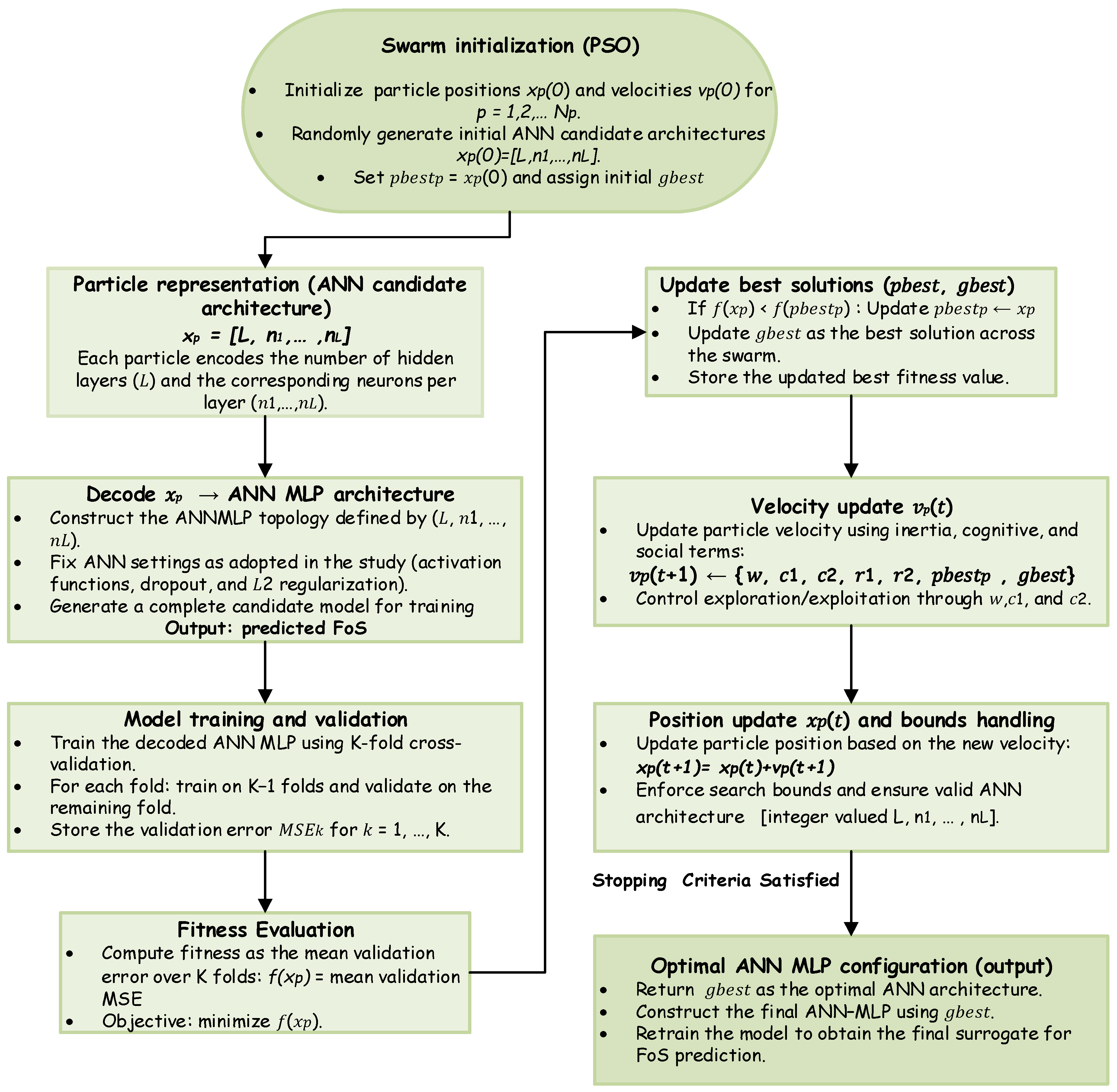
Through repeated velocity and position updates, the swarm progressively explores the ANN hyperparameter space and identifies the best-performing configuration within the tested search domain. The resulting global-best solution (gbest) is subsequently used to retrain the ANN using the full training dataset [80,81,82,83]. Figure 2 illustrates the PSO-driven workflow adopted for ANN hyperparameter optimization. Each particle encodes a candidate network configuration, which is decoded into an ANN–MLP and evaluated using K-fold cross-validation. The resulting fitness value guides the PSO velocity and position updates while enforcing the prescribed bounds and integer constraints on the architecture variables. The iterative search process continues until the stopping criterion is satisfied, after which the best-performing configuration identified during the search is retained for final ANN training.

2.2. Application Using Python

The proposed ANN–MLP–PSO framework was implemented in Python and applied to a final dataset of 2014 homogeneous slope cases. The dataset was constructed from two complementary sources: 705 literature-derived cases, representing approximately 35.0% of the database, and 1309 numerically generated cases, representing approximately 65.0% of the database. The literature-derived cases were compiled from published slope stability studies that reported the required input variables, namely slope height H, slope angle θ, pore-water pressure ratio R_u, unit weight γ, cohesion c, friction angle ϕ, and the corresponding factor of safety (FoS). Cases with missing input variables, inconsistent units, unclear slope geometry, duplicated records, or incomplete FoS information were excluded before model development. The numerically generated cases were introduced to improve coverage of the geotechnical input space and reduce the uneven parameter distribution commonly observed in published slope stability datasets. In the simulation-based augmentation stage, the six input variables (H, θ, R_u, γ, c, ϕ) were systematically varied within geotechnically admissible ranges selected to cover both dry and wet homogeneous slope conditions. The corresponding reference FoS values were computed using conventional slope stability analysis procedures based on limit equilibrium analysis using SLOPE/W (GeoStudio 2021) software and finite element analysis using PLAXIS 2D. Therefore, the generated cases were not assigned arbitrary FoS values; each output FoS was obtained from a mechanics-based slope stability calculation.

Before merging, both data subsets were organized using an identical structure comprising the same six input variables and FoS output. Variable definitions and measurement units were harmonized across the two sources, including slope heights in meters, slope and friction angles in degrees, unit weights in kN/m³, cohesion in kPa, and the dimensionless pore-water pressure ratio. The validated records were subsequently concatenated into a unified database of 2014 cases. The data-source category was not included as an ANN input. Therefore, the literature-derived and numerically generated cases were treated consistently during subsequent model development.

The final dataset spans wide ranges of the six input variables and the output FoS, ensuring that model training is not biased toward a narrow subset of slope conditions. The six input parameters were slope height H ranging from 1.10 to 511 m, slope angle θ ranging from 14° to 90°, pore-water pressure ratio Ru ranging from 0.00 to 0.85, unit weight γ ranging from 12.0 to 31.3 kN/m³, cohesion c ranging from 0 to 155 kPa, and friction angle ϕ ranging from 0° to 45°. The output variable was the factor of safety, ranging from 0.04 to 4.994.

Table 1. Descriptive Statistics of the Slope Stability input dataset and FoS values.

Parameter	Min	Max	Mean	Std. Dev.	Mode	COV (%)
Slope Height (m)	1.10	511.00	35.53	69.39	10.00	195.29
Slope Angle θ (°)	14.00	90.00	33.92	11.44	45.00	33.73
Pore Water Pressure Ratio Ru	0.00	0.85	0.275	0.210	0.00	76.60
Unit Weight γ (kN/m3)	12.00	31.30	18.50	2.66	18.00	14.35
Cohesion c (kPa)	0.00	155.00	26.26	24.37	10.00	92.80
Friction Angle ϕ (°)	0.00	45.00	23.54	9.16	28.00	38.91
Factor of Safety FoS (-)	0.04	4.994	1.534	0.965	1.11	62.94

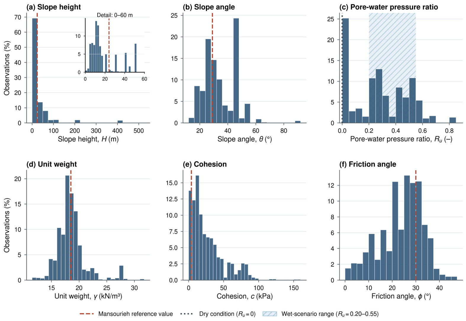
reports the descriptive statistics of the database variables. To assess the applicability of the global training database to the field application considered later in this study, Figure 3. indicates the reference input values adopted for the Mansourieh slope and the prescribed dry and wet hydraulic conditions. The case study geometry, geotechnical parameters, and probabilistic characterization are presented in Section 4. 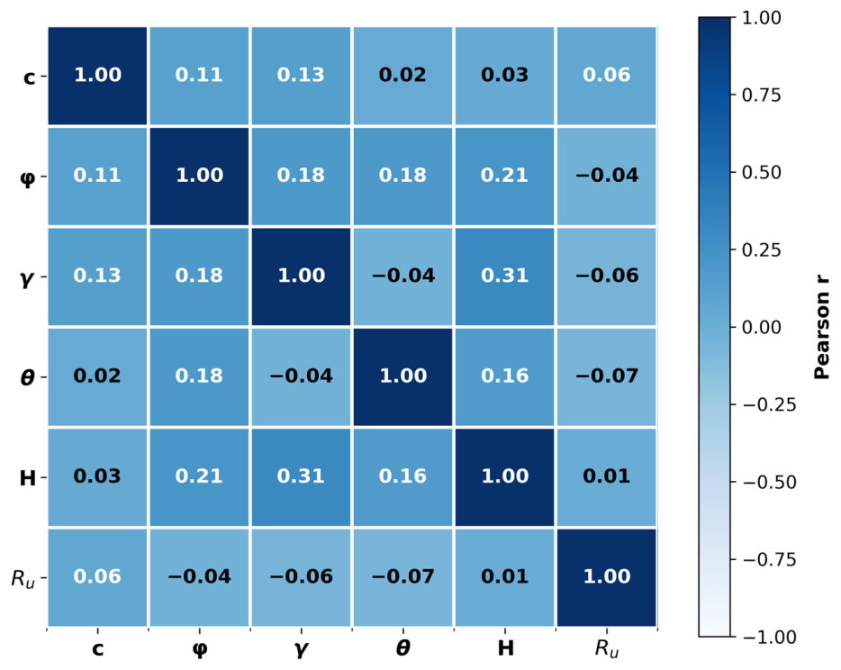Figure 4. presents the Pearson correlation heatmap of the six ANN input variables.

Although the slope heights in the database range from 1.10 to 511 m and exhibit a COV of 195.29%, Figure 3a shows that the empirical distribution is strongly right-skewed rather than uniformly distributed over this interval. The median, 75th-percentile, and 90th-percentile slope heights are 12, 31, and 50 m, respectively, and 1830 of the 2014 cases (90.86%) have heights not exceeding 50 m. The Mansourieh slope height of 24 m lies at approximately the 69th percentile of the database, with 214 cases (10.63%) occurring between 20 and 30 m. Therefore, the maximum height of 511 m represents a sparsely populated upper tail, whereas the Mansourieh case does not require extrapolation with respect to slope height. The adopted Mansourieh geometric, geotechnical, and hydraulic reference values also lie within the corresponding empirical input ranges, as illustrated in Figure 3. Differences in the numerical magnitudes of the input variables were addressed through z-score standardization fitted exclusively to the training subset, thereby preventing variables with larger raw numerical scales from disproportionately influencing ANN optimization.

Although these distributional characteristics demonstrate that the Mansourieh case does not require direct range extrapolation, inclusion within the global database bounds does not by itself establish that a surrogate trained across the complete height range provides locally stable predictions for a 24 m slope. Therefore, an additional height-domain robustness analysis was conducted using only cases with 10 ≤ H ≤ 50. This predefined interval excludes very small slopes that are not comparable in scale with Mansourieh, retains the densely populated portion of the database up to its 90th-percentile height, and provides a sufficiently large subset for independent training and testing. The methodology and results of this assessment are presented in Section 4.3.

After database assembly and quality control, the 2014 cases were randomly divided into training and testing subsets using an 80/20 split with a fixed random seed (random_state = 42). To prevent information from the held-out testing subset from influencing model development, z-score scaling was fitted exclusively to the 80% training subset. For each input variable, the mean and standard deviation calculated from the training subset were used to transform the training data, and the same fitted scaling parameters were subsequently applied without modification to the held-out testing subset. During PSO-based hyperparameter and architecture selection, shuffled five-fold cross-validation was performed within the training subset using the same fixed random seed. The held-out 20% testing subset remained excluded from ANN training, PSO fitness evaluation, and hyperparameter selection and was used only for final assessment of the model’s generalization. The z-score transformation may also be shown explicitly

$$x_{i,scaled}={\displaystyle \frac{x_i-{\mu }_{i,train}}{{\sigma }_{i,train}}}$$

(8)

where μ_i,train and σ_i,train are the mean and standard deviation of input variable i, calculated exclusively from the training subset.

Following PSO convergence, the best-performing configuration was retrained using the complete training subset, and its predictive performance was evaluated on the held-out 20% testing subset, which was not used during model training or hyperparameter selection. Early stopping was not employed. Instead, dropout and L2 regularization were used to control model complexity and reduce overfitting. A fully connected ANN–MLP was adopted, using tanh activation in the first hidden layer and ReLU activation in subsequent layers to capture nonlinear relationships between the geotechnical inputs and the FoS output. The output layer employed a linear activation function to generate continuous FoS predictions. Regularization measures (dropout and L2 weight decay) were incorporated to enhance generalization. PSO was then used to identify the most effective ANN hyperparameter configuration, where each particle represented a candidate architecture and training setup (number of hidden layers, neurons per layer, batch size, and epochs). At each PSO iteration, particles updated their positions based on individual best performance and swarm best performance, progressively converging toward the optimal ANN configuration, which was subsequently adopted for final prediction and benchmarking analyses. All computational experiments were performed in Python 3.12.7 using TensorFlow 2.19.0 on a Windows 11 system. The workstation was equipped with an Intel Core i7-10750H CPU (Intel Corporation, Santa Clara, CA, USA) and 12 GB RAM. All ANN training, PSO optimization, and probabilistic surrogate simulations were performed using CPU computation only; GPU acceleration was not used.

3. Probabilistic Reliability Framework

3.1. ANN Surrogate-Based Probabilistic Post-Processing

Following hyperparameter optimization and validation, the best-performing ANN–MLP–PSO model was retained as the deterministic surrogate of the slope stability response. To perform probabilistic reliability assessment, the optimized ANN was embedded within a Monte Carlo-type sampling framework and evaluated without further retraining. Random input vectors were generated according to the prescribed probability distributions of the geotechnical variables and propagated through the fixed ANN surrogate to obtain a distribution of predicted factors of safety (FoS).

The resulting FoS distribution was used to compute the probability of failure (P_f), defined as the proportion of realizations with FoS < 1, the corresponding reliability index (β = −Φ⁻¹(P_f)), and the characteristic FoS quantiles (FoS5%, FoS50%, and FoS95%). Because uncertainty propagation is performed through the ANN surrogate rather than repeated deterministic slope stability analyses, the procedure provides a computationally efficient surrogate-based approach for probabilistic reliability assessment while maintaining consistency with the probabilistic framework adopted for the benchmark reliability methods.

To ensure direct benchmarking, the same probabilistic characterization of the input variables adopted in the FOSM, PEM, and MCS analyses was used during ANN-based sampling. The reliability metrics obtained from the ANN should therefore be interpreted as surrogate-based probabilistic estimates conditioned on the trained ANN approximation. Epistemic uncertainty associated with model training, surrogate approximation, and potential extrapolation beyond the training domain was not explicitly propagated into the reported reliability metrics. For each hydraulic condition (dry and wet cases), 20,000 ANN-based sampling realizations were generated.

3.2. Deterministic Formulation and Limit-State Definition

Deterministic slope stability is evaluated using the Morgenstern–Price (MP) limit equilibrium method, which satisfies both global force and moment equilibrium for a trial slip surface [84]. Interslice forces are linked through the Morgenstern–Price functional relationship

$$T\left(x\right)=\lambda f\left(x\right)N\left(x\right)$$

(9)

where $T\left(x\right)$ and $N\left(x\right)$ denote interslice shear and normal forces, respectively, $f\left(x\right)$ is the interslice force function, and $\mathit{\lambda }$ is an unknown scaling parameter solved simultaneously with the factor of safety. For reliability analysis, the slope problem is cast in a limit-state form by defining the random variable vector $X = {\left[c, \phi , \gamma , R_u\right]}^T$, whereas the slope geometry is treated as deterministic and the limit-state function:

$$g\left(X\right)= F\left(X\right)- 1$$

(10)

where $F\left(X\right)$ is the computed factor of safety. Failure is defined by $g\left(X\right)$ ≤ 0 [85,86].

Pore-water pressures are incorporated using the conventional pore pressure ratio method:

$$u_i= R_u\gamma z_i$$

(11)

where $u_i$ is the pore pressure at the base of slice i, ${\mathit{z}}_{\mathit{i}}$ is the depth from ground surface to the centroid of the slice base, and $\gamma$ is the total unit weight [7,84,87]. The effective normal stress is then:

$${\sigma }_n^{\prime }= {\sigma }_n- u_i$$

(12)

Figure 5 provides a visual illustration of the reliability concept adopted in this study. It illustrates the failure threshold and the associated failure probability in both the FoS domain and the limit-state space.

3.3. Probabilistic Characterization of Input Parameters

Uncertainty in soil parameters was represented using probabilistic models selected to reflect physical constraints and empirical geotechnical practice. Cohesion (c) was modeled as lognormal to enforce non-negativity, with parameters derived from the prescribed mean and coefficient of variation. The friction angle (ϕ) and unit weight (γ) were modeled using normal distributions. Pore pressure ratio${(R}_u)$ was treated as deterministic in dry conditions ($R_u=0$), while for wet conditions it was bounded within a practical envelope R_u ∈ [0.20, 0.55] [7,88] and modeled using a triangular distribution with mode at 0.4, reflecting bounded support and limited-information uncertainty. Unless site-specific correlation data are available, the variables in $X = {\left[c, \varphi , \gamma , R_u\right]}^T$ were assumed independent, consistent with standard reliability modeling practice for homogeneous slopes [88]. The adopted triangular R_u distribution (0.20, 0.40, 0.55) was selected to represent moderate-to-high wet-condition hydraulic degradation commonly encountered in practical slope stability reliability analyses and to remain consistent with the observed rainfall-sensitive behavior of the Mansourieh slope. The selected range was intended to provide a generalized probabilistic representation of elevated pore-pressure conditions rather than a site-specific transient seepage calibration. The same R_u characterization was consistently applied to ANN–MLP–PSO, MCS, FOSM, and PEM to ensure fair probabilistic benchmarking between all methods.

In the present study, the uncertain input variables were assumed to be statistically independent to maintain methodological consistency across the ANN–MLP–PSO, MCS, FOSM, and PEM reliability analyses. Although statistical dependence may exist between certain geotechnical parameters, particularly among shear-strength and density-related variables, the independence assumption is widely adopted in homogeneous slope reliability studies when detailed joint probabilistic characterization is unavailable. This assumption enables a consistent comparison among the investigated reliability approaches while preserving a transparent probabilistic framework.

3.4. Benchmark Reliability Methods

To establish a rigorous probabilistic baseline and enable direct comparison with the proposed ANN–MLP–PSO surrogate framework, three benchmark reliability techniques were implemented: Monte Carlo simulation (MCS), the First-Order Second-Moment method (FOSM), and the Point Estimate Method (PEM). Among these approaches, MCS was adopted as the reference probabilistic benchmark because it directly propagates input uncertainty through repeated random sampling without relying on response linearization or moment-based approximations, thereby providing a more complete representation of the probabilistic response. Accordingly, uncertainty was propagated through repeated sampling of the random variable vector X = [c, ϕ, γ, Ru]^T. For each realization, the deterministic Morgenstern–Price solver returns a factor of safety, and the limit-state function is evaluated. $\left\{X^{\left(j\right)}\right\}\begin{array}{c}N\\ \mathrm{j}=1\end{array}{F}^{\left(j\right)}{g\left(X\right)}^{\left(j\right)}= F^{\left(j\right)}-1$. Failure probability and reliability index are estimated as:

$${\widehat{P}}_f= \left({\displaystyle \frac{1}{N}}\right){\displaystyle {\sum }_{j=1}^N}I \left\{F^{\left(j\right)}< 1\right\} ,\widehat{\beta }= {\Phi }^{-1}\left(1 - {\widehat{P}}_f\right)$$

(13)

where $\Phi$ is the standard normal Cumulative Distribution function CDF, I(⋅) is the indicator function, and N is the number of simulations. Beyond mean and variance, quantiles of FoS $\left({FoS}_5\%, {FoS}_{50}\%, {FoS}_{95}\%\right)$ and full cumulative distribution are reported [89,90]. For consistency with the ANN surrogate probabilistic analyses, 20,000 Monte Carlo realizations were used in the benchmark MCS simulations.

The First-Order Second-Moment method (FOSM) was employed as an efficient approximation technique based on linearization of the response function around the mean input vector μ = E[X]. E[⋅] denotes the expectation operator. The factor of safety is approximated by a first-order Taylor expansion:

$$F\left(X\right)\approx F\left(\mu \right)+ \nabla F{\left(\mu \right)}^{\mathrm{T}} \left(X - \mu \right)$$

(14)

for which the FoS mean and variance are as essential as ${\mu }_F\approx F\left(\mu \right)$ and:

$${\sigma }_F^2\approx \nabla F{\left(\mu \right)}^{\mathrm{T}}{\sum }_X \nabla F\left(\mu \right)$$

(15)

where ${\sum }_{\mathit{X}}$ is the covariance matrix of inputs. Under the standard normal approximation, the reliability index and probability of failure are computed as:

$$\beta \approx {\displaystyle \frac{{\mu }_F- 1}{{\sigma }_F}},P_f\approx \Phi \left(-\beta \right)$$

(16)

where $\Phi$ is the standard normal cumulative distribution function (CDF). This formulation enables rapid reliability assessment while providing sensitivity insight through the gradient terms [17,91].

The Point Estimate Method (PEM) was implemented as a computationally efficient alternative to MCS by evaluating the deterministic solver at a limited set of representative points in the input space. For the random vector X with n independent variables, PEM requires a finite number of solver evaluations to approximate the first two moments of the factor of safety distribution. In this study, Rosenblueth’s 2n point estimate scheme (two-point PEM) was adopted, requiring 2n deterministic solver evaluations for n random variables. The mean and variance of FoS are estimated using weighted combinations of the evaluated responses:

$${\mu }_F\approx {\sum }_K{ \omega }_{k}F\left(x^{\left(k\right)}\right)$$

(17)

$${\sigma }_F^2\approx {\sum }_K{\omega }_k{\left(F\left(x^{\left(k\right)}\right)-{\mu }_F\right)}^2$$

(18)

with uniform weights${ \omega }_k= 2^{-n}.$ Reliability outputs are then computed as:

$$\beta =\left({\mu }_F-1\right)/{\sigma }_F,P_f=1-\Phi \left(\beta \right)$$

(19)

where Φ is the standard normal cumulative distribution function (CDF). PEM provides reliable estimates of ${\mu }_F$, ${\sigma }_F$, and FoS quantiles at substantially reduced computational cost relative to MCS [89,92]. For clarity and consistency, a single sign convention is used throughout: for any method, β = −Φ⁻¹(P_f), which is equivalent to P_f = Φ(−β). For sampling-based methods (MCS and ANN sampling), P_f is estimated directly from failure counts (FoS < 1) and β is then computed from P_f. For moment-based methods (FOSM and PEM), β is computed from (μ_F, σ_F) and P_f is subsequently derived as P_f = Φ(−β).

4. Case Study

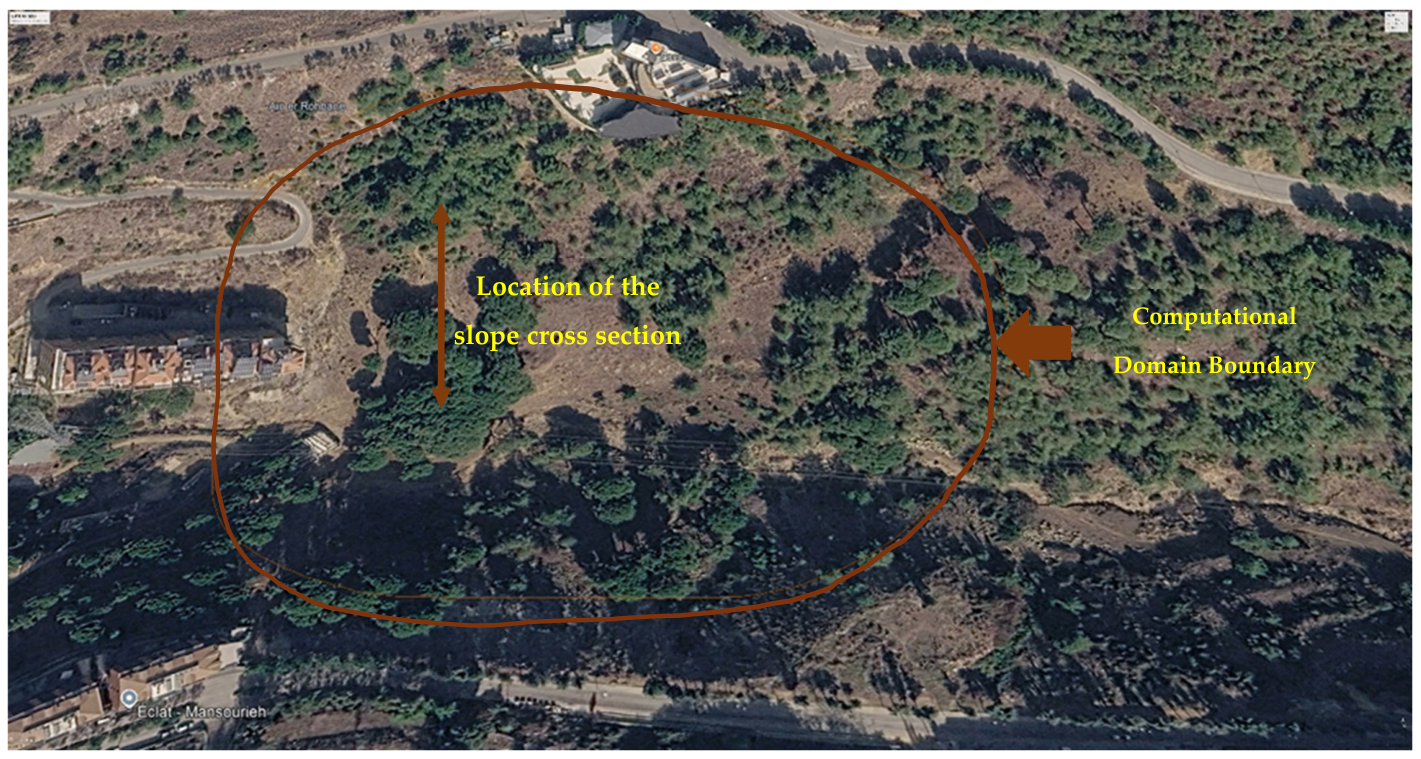
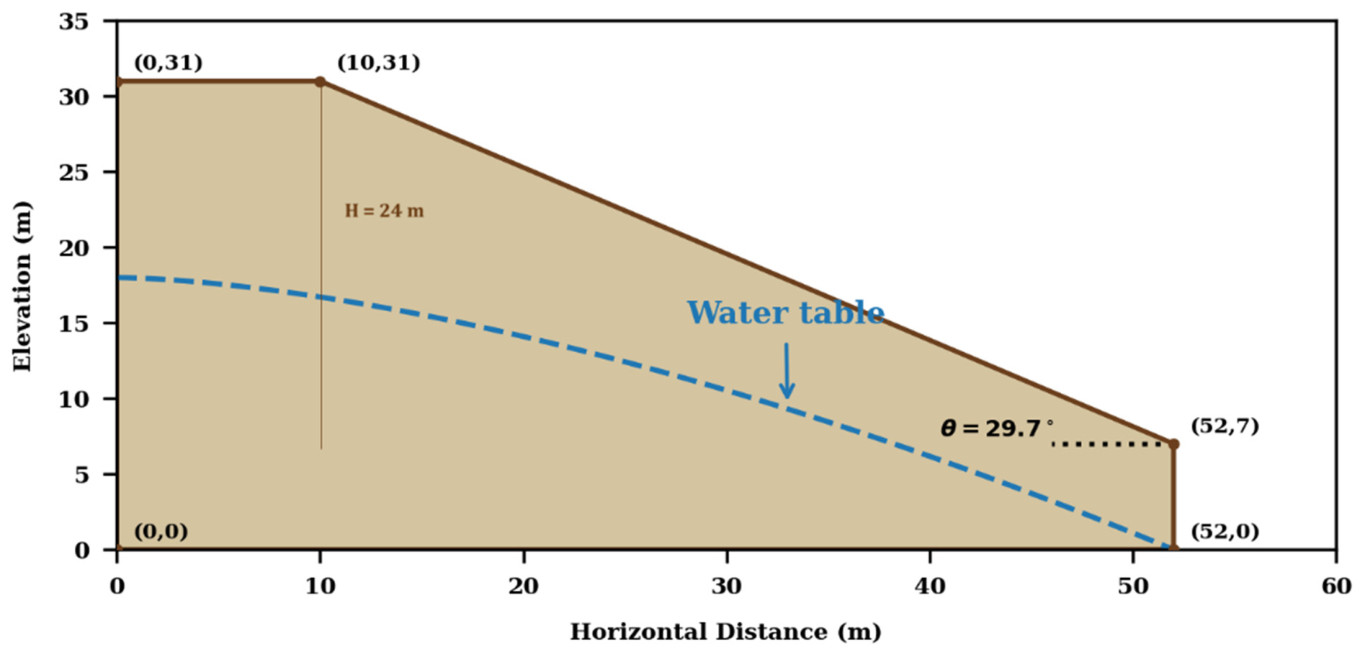
The case study investigated in this research is the Mansourieh slope, located in the eastern suburbs of Beirut, Lebanon, near 33°51′45″ N and 35°33′48″ E. Figure 6 presents a high-resolution Google Earth image of the site, indicating the approximate boundary of the computational domain and the location and orientation of the analyzed cross-section. Figure 7 shows the two-dimensional computational slope domain adopted for the slope stability analyses in a local horizontal–vertical coordinate system. The modeled slope has a height of H = 24 m and a face inclination of θ = 29.7°. The corresponding phreatic surface is also shown. The slope extends over an area of approximately 500 m × 200 m, reaching an elevation of about 154 m above mean sea level. Geologically, the site lies within a Cretaceous formation overlying the Siliceous Nubian Sandstone (“Grès de Nubie Siliceux”), and the soil mass consists mainly of sandy clay and clayey sand, with minor gravel inclusions and locally a thin expansive clay layer (“Roumieh clay”) at depths of approximately 6–7.5 m. Geotechnical characterization was established using field investigations including a Standard Penetration Test (SPT) and Shear Resistance Test (SRT) and laboratory analyses such as grain-size distribution and direct shear testing. The investigations indicate that the soil profile belongs to the same geologic unit and exhibits consistent mechanical behavior, supporting the treatment of the slope as a homogeneous soil system for deterministic and probabilistic analyses [93].

The documented history of the Mansourieh slope does not indicate an unequivocally stable condition. The published site investigation reported slope movement in 1994 and noted that although the slope appeared stable at the time of that investigation, its stability remained critical [93]. The corresponding three-dimensional static analysis produced an FoS of approximately 1.1 in critical zones and identified two relatively weak areas. One zone corresponded to the location of the 1994 movement, whereas the second had not experienced documented movement at the time of the investigation [93].

Two climatic scenarios were considered to represent seasonal pore-pressure conditions: (i) a dry case with R_u = 0 and (ii) a wet case where R_u is treated probabilistically to capture rainfall-induced pore pressure rise. The slope geometry is treated as deterministic. Specifically, the slope height H and inclination angle θ are fixed to the Mansourieh configuration, while uncertainty is modeled only in the geotechnical and hydraulic parameters. Therefore, random samples are generated for X = [c, ϕ, γ, R_u]^T, and each sampled realization is combined with the fixed (H, θ) values before being propagated through the trained ANN (whose full input vector is [H, θ, R_u, γ, c, ϕ]). This ensures consistent use of the limit-state definition g(X) = F(X)−1 for all techniques. The wet-condition R_u distribution was adopted as a generalized conditional hydraulic scenario and was not derived from site-specific piezometric or pore-water pressure monitoring at Mansourieh. Accordingly, the resulting wet-condition probabilities of failure quantify the response conditional on the adopted R_u range and should not be interpreted as estimates of the current or annual field probability of failure. A measurement-based recalculation was not performed because suitable time-dependent site pore-water pressure records were unavailable. The probabilistic characterizations of input parameters for both cases are listed in

Table 2. Probabilistic input parameter distributions and statistics for dry and wet cases.

Parameter	Distribution	Dry Case	Wet Case
Cohesion c (kPa)	Lognormal	μ = 4.0, SD = 2.0, COV = 50%	μ = 4.0, SD = 2.0, COV = 50%
Friction angle ϕ (°)	Normal	μ = 30, σ = 3.0, COV = 10%	μ = 30, σ = 3.0, COV = 10%
Unit weight γ (kN/m3)	Normal	μ = 18.5, σ = 1.30, COV = 7%	μ = 18.5, σ = 1.30, COV = 7%
Pore-Water Pressure Ru	Triangular	—	min = 0.20, mode = 0.40, max = 0.55

.

The Mansourieh slope was used as an application case for the trained ANN–MLP–PSO surrogate and was not included as a source of model training data. Its adopted geometry, comprising H = 24 m and θ = 29.7°, falls within the corresponding global database ranges of 1.10–511 m and 14–90°, respectively. The adopted mean values of cohesion (μ = 4.0 kPa), friction angle (μ = 30°), and unit weight (μ = 18.5 kN/m³) also fall within the corresponding database ranges of 0–155 kPa, 0–45°, and 12.0–31.3 kN/m³. Similarly, the dry condition (R_u = 0) and the wet-scenario range (R_u = 0.20–0.55) fall within the global database range of 0.00–0.85 (

Table 3. Comparison between the Mansourieh case study inputs and the applicability domain of the global ANN training database.

ANN–MLP–PSO Input	Global Database Range	Mansourieh Condition	Within Database Domain?
Slope height H (m)	1.10–511	24	Yes
Slope angle θ (°)	14–90	29.7	Yes
Cohesion c (kPa)	0–155	Lognormal: (μ = 4.0), SD (=2.0)	Yes, based on the adopted central values
Friction angle ϕ (°)	0–45	Normal: (μ = 30), SD (=3.0)	Yes, based on the adopted central values
Unit weight γ (kN/m3)	12.0–31.3	Normal: μ = 18.5), SD (=1.3)	Yes, based on the adopted central values
Pore-water pressure (Ru)	0.00–0.85	Dry: (Ru = 0); wet: 0.20–0.55	Yes

). Thus, the global database was used to develop the ANN surrogate, whereas the Mansourieh slope was subsequently used to demonstrate its case-specific application.

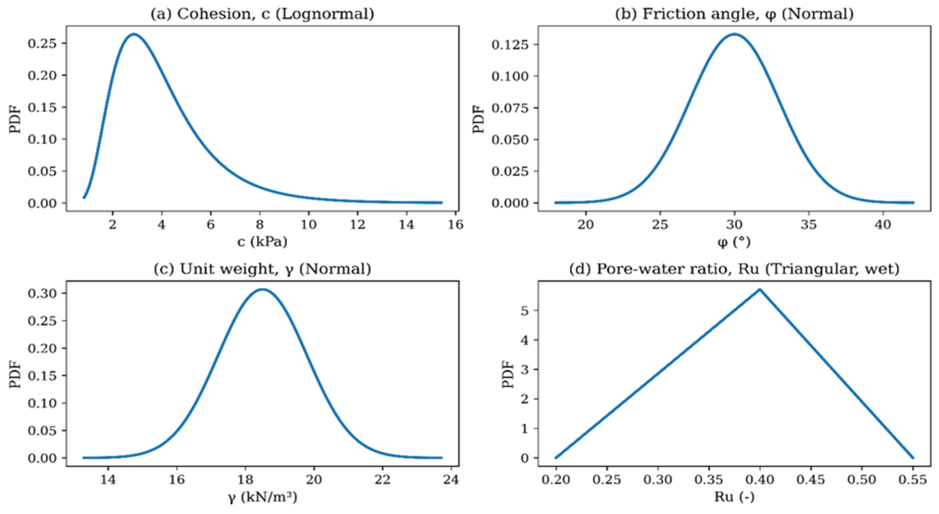
Figure 8 presents the probabilistic characterization adopted for the geotechnical input variables. The selected distributions reflect the assumed uncertainty in shear strength parameters, unit weight, and pore-water pressure conditions used in the reliability analyses.

4.1. Results and Outputs

4.1.1. Sensitivity Analysis for PSO Coefficients

In PSO, particle dynamics are governed by the cognitive coefficient c₁ (self-learning), the social coefficient c₂ (swarm learning), and the inertia weight ω (velocity persistence). A coefficient sensitivity study was conducted by varying (c₁,c₂,ω) while holding all other PSO and ANN settings constant. Because each fitness evaluation requires 5-fold cross-validation training, this analysis was designed as a comparative screening under a fixed computational budget rather than an exhaustive convergence study. The fixed settings were swarm size = 10, iterations = 5, K = 5, hidden layers L ∈ [4,6], neurons per layer n_ℓ ∈ [72,96], batch size = 32, and epochs = 400.

A broader coefficient sweep was performed.

Table 4. Sensitivity analysis of Particle Swarm Optimization coefficients.

Cognitive Coefficient (c1)	Social Coefficient (c2)	Inertia Weight (ω)	R2	MAE	RMSE	MSE	Network Structure
1.5	1.8	0.6	0.89	0.41	0.64	0.41	[80, 81, 82, 85, 89, 80]
1	1	0.5	0.87	0.47	0.69	0.48	[87, 84, 76, 85, 88, 86]
1.2	1.5	0.6	0.79	0.79	0.89	0.79	[96, 88, 82, 84, 79, 91]
1.5	1.2	0.7	0.95	0.17	0.41	0.17	[82, 77, 91, 79, 78, 84]
1.8	1.5	0.8	0.94	0.22	0.47	0.23	[93, 83, 83, 79, 88, 76]
2	1	0.6	0.94	0.21	0.60	0.37	[93, 95, 73, 90, 87, 75]
1.5	1.8	0.5	0.94	0.23	0.47	0.22	[86, 76, 90, 96, 77, 81]
2.2	1.5	0.3	0.87	0.48	0.69	0.48	[89, 86, 81, 80, 89, 79]
1.8	2	0.7	0.93	0.26	0.51	0.26	[94, 94, 78, 88, 82, 73]
2.5	2.5	0.9	0.95	0.19	0.44	0.192	[85, 86, 78, 76, 73, 92]

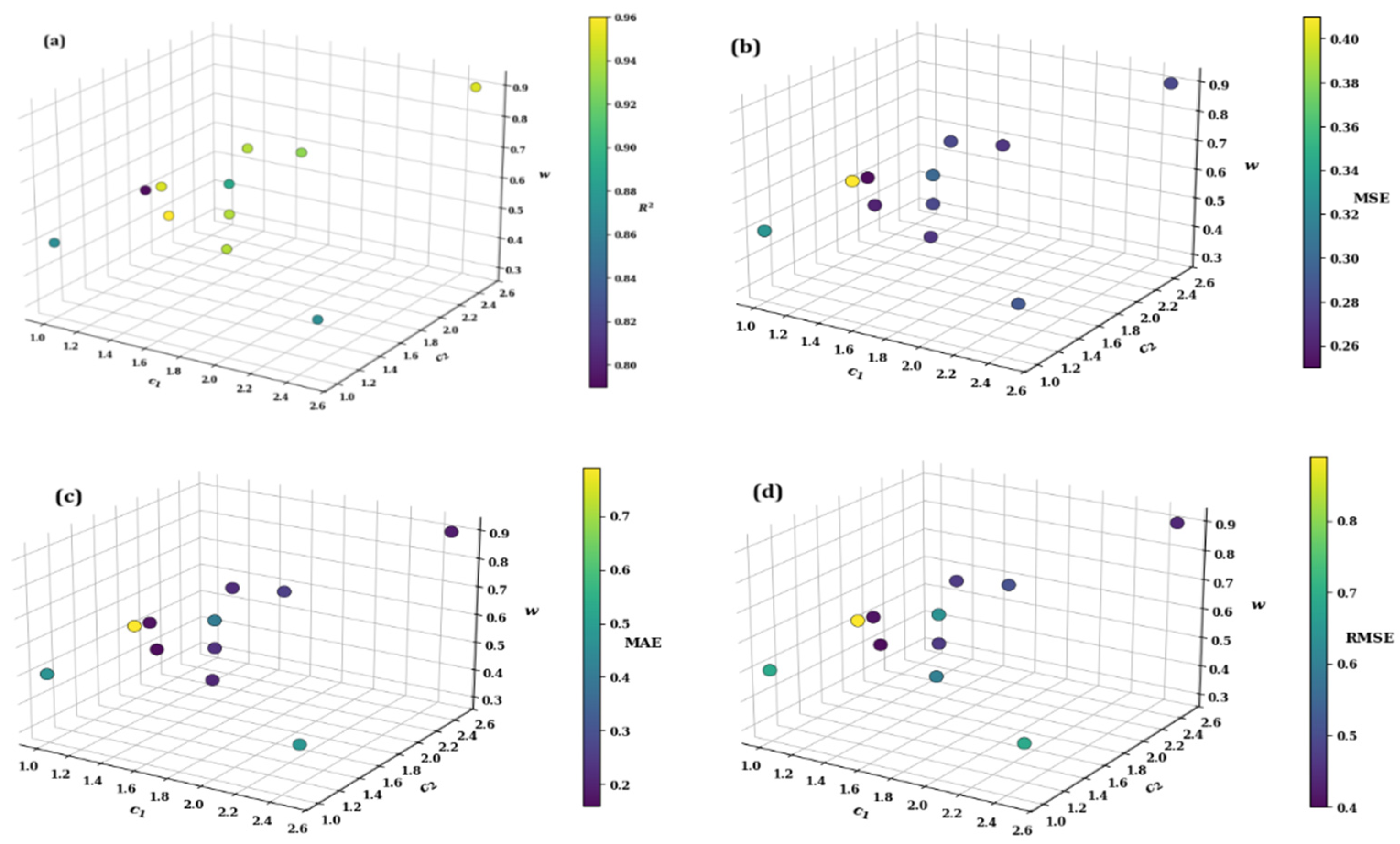
reports the top configurations ranked primarily by R². The best-performing triplet (c1,c2,ω) = (1.5,1.2,0.7) achieved R2 = 0.95, MAE = 0.17, and RMSE = 0.41 and was adopted for subsequent PSO-based optimization runs. Network structure denotes the optimized hidden-layer neuron vector [n1, …, nL] returned by PSO for each coefficient triplet.

The 3D sensitivity maps in Figure 9 indicate that performance depends on balancing exploration and exploitation. Higher R² values are generally obtained for moderate-to-high inertia weights combined with balanced acceleration coefficients, consistent with improved convergence stability and reduced risk of premature stagnation. The corresponding R²/MAE/RMSE/MSE maps confirm the same region as error-minimizing, supporting the robustness of the selected coefficients.

4.1.2. Network Training and Evaluation

Model performance was evaluated using the coefficient of determination (R²), root mean square error (RMSE), and mean absolute error (MAE), as defined previously. The adopted ranges of the optimized hyperparameters and the PSO control parameters are summarized in

Table 5. Selected hyperparameters ranges for the ANN–MLP–PSO model optimization.

Hyperparameter	Number of Hidden Layers	Neurons per Layer	Batch Size	Epochs	Swarm Size (PSO)	Iterations (PSO)
Range	2–6	8–96	16–64	20–2000	10–80	5–50

.

The PSO-based architecture selection and cross-validation procedure constituted a one-time model-development stage. For each candidate particle, the mean validation MSE across the five folds, combined with the reliability-oriented correction term defined in Equation (5) was used as the fitness value. After selection of the global-best particle, the corresponding architecture and training hyperparameters were fixed and the network was retrained on the complete training subset without further hyperparameter adjustment. The resulting trained surrogate was subsequently used without additional weight updates for held-out testing and probabilistic input propagation, for which each realization required only a forward ANN evaluation.

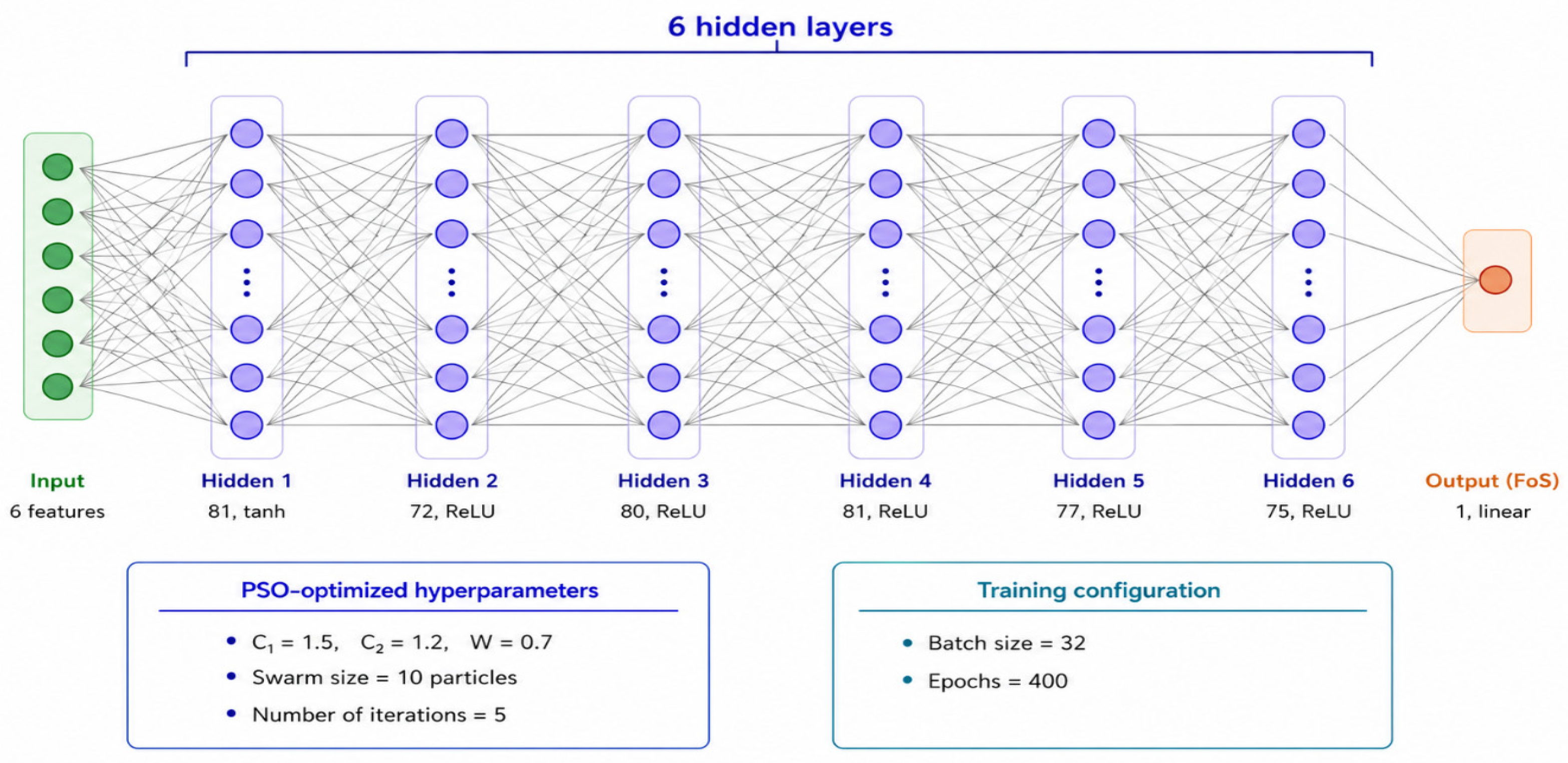
The six-hidden-layer architecture was selected through systematic hyperparameter optimization rather than by arbitrary choice. Network depth was explored over the predefined range of two to six hidden layers, jointly with the number of neurons per layer, batch size, and number of training epochs. The selected configuration comprised six hidden layers and used 30 epochs during fold-level fitness evaluation and 400 epochs during final model training, as reported in Table 5. Thus, the number of epochs was treated as an optimized training hyperparameter within the investigated search space rather than as a dynamically terminated training procedure. Overfitting was further mitigated through a dropout rate of 0.1 and L2 weight decay of 0.001. The generalization capability of the final model was evaluated using the independent hold-out test subset, complemented by predicted versus observed comparisons and residual-error analysis. Early stopping was not applied because training duration was governed by the evaluated epoch settings and the predefined regularization measures. However, its incorporation may be examined in future extensions of the framework.

Table 6. Top ten performing ANN–MLP–PSO configurations and associated performance metrics.

Case	Epochs (E1, E2)	Layers Range	Neurons Range	Particles	Iterations	R2	MAE	RMSE	MSE	Network Structure
1	30, 500	[4,6]	[72–96]	12	5	0.95	0.19	0.44	0.194	[88, 86, 88, 76, 78, 84]
2	30, 400	[4,6]	[72–96]	10	5	0.95	0.19	0.43	0.185	[81, 72, 80, 81, 77, 75]
3	20, 500	[4,6]	[48–96]	20	10	0.92	0.28	0.55	0.30	[72, 74, 93, 59, 65, 72]
4	20, 500	[4,6]	[8–64]	10	5	0.92	0.28	0.52	0.27	[54, 56, 42, 51, 31, 34]
5	30, 700	[4,6]	[8–96]	10	5	0.91	0.33	0.58	0.34	[84, 46, 87, 62, 95, 21]
6	20, 600	[4,6]	[8–64]	10	5	0.90	0.36	0.60	0.36	[61, 37, 52, 50, 47, 28]
7	30, 500	[4,6]	[8–96]	10	5	0.90	0.35	0.59	0.35	[47, 54, 50, 36, 47, 22]
8	30, 300	[2,4]	[20–30]	20	8	0.90	0.37	0.61	0.37	[27, 24, 25, 29]
9	50, 350	[2,4]	[20–35]	25	8	0.90	0.38	0.61	0.37	[35, 31, 32, 31]
10	20, 1000	[4,6]	[8–64]	10	5	0.89	0.41	0.64	0.41	[64, 60, 61, 44, 21, 42]

presents the ten best-performing ANN–MLP–PSO configurations obtained from the hyperparameter optimization runs. Overall, the results indicate that predictive performance is primarily governed by the network architecture, whereas increasing the PSO search budget beyond modest levels yields only marginal improvements. The highest-ranking models consistently correspond to deeper MLP structures comprising six hidden layers with moderate-to-high widths, typically ranging between 72 and 96 neurons per layer. Although the PSO search space included swarm sizes from 10 to 80 particles and iteration numbers from 5 to 50, the best-performing tested configuration was obtained using a relatively small PSO budget. This does not imply that a small PSO budget is universally sufficient, nor that a global optimum was mathematically guaranteed. Rather, within the explored configurations, increasing the swarm size or the number of iterations did not produce a better validation–testing trade-off. The selected configuration is therefore interpreted as the best-performing model among the tested PSO settings under the adopted cross-validation procedure. In contrast, more compact architectures with fewer hidden layers remained competitive, achieving R² values close to 0.90, but exhibited noticeably higher residual errors (RMSE ≈ 0.61), reflecting reduced representational capacity. Furthermore, the lowest-ranked configuration, which employed prolonged training with 1000 epochs, did not lead to improved accuracy and instead resulted in weaker generalization. This behavior suggests that excessive training may increase the risk of memorization rather than enhancing predictive robustness. Collectively, these findings indicate that network architecture exerted a stronger influence on predictive performance than further increases in the PSO search budget, with the highest-performing configurations consistently corresponding to deeper ANN structures within the explored search space. The absence of systematic improvement with larger swarm sizes or iteration counts suggests that increasing the PSO search budget beyond the tested levels did not necessarily enhance ANN generalization performance for the present dataset.

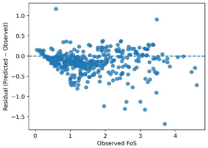
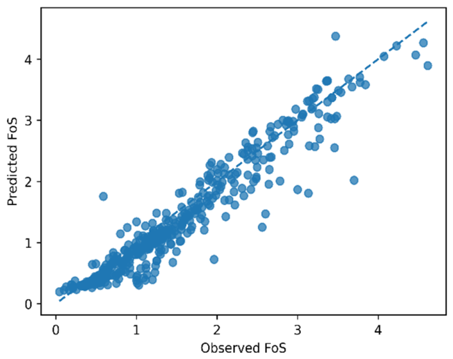
Figure 10 and Figure 11 illustrate the predictive performance of PSO-optimized ANN–MLP of the test dataset. The predicted–observed scatter plot demonstrates strong agreement between model predictions and reference FoS values, with limited dispersion across the full range. The corresponding residual plot confirms that prediction errors remain centered around zero without any evident systematic bias, supporting the robustness of the trained model. The final ANN–MLP architecture adopted in this study is illustrated in Figure 12. This figure reports the selected hidden-layer sizes and activation functions, along with the PSO coefficients and training configuration used to obtain the optimal predictive model for FoS estimation.

Computational efficiency was quantified through wall-clock benchmarking on the hardware described in Section 2.2 (Intel Core i7-10750H CPU, 12 GB RAM, CPU-only execution) in addition to comparing the number and type of response-model evaluations required during probabilistic propagation. The direct MCS analysis required 20,000 evaluations of the deterministic slope stability model, one for each probabilistic realization, and this analysis required 25 min to complete. In contrast, after the one-time PSO optimization and ANN training stage, which required 10 min, the ANN-based analysis propagated the same 20,000 realizations through the fixed surrogate using forward network evaluations without repeating the deterministic slope stability calculation. This probabilistic propagation stage required 3 min. Accordingly, once trained, the ANN–MLP–PSO surrogate reduced the probabilistic evaluation runtime by a factor of approximately 8 relative to direct MCS, while the one-time training cost is incurred only during model development and is amortized over any subsequent reuse of the surrogate.

4.2. Comparative Reliability Outputs (Dry and Wet Cases)

Table 7. Dry case probabilistic reliability outputs and FoS quantiles.

Technique	Mean FoS μF	Std. Dev. FoS σF	COV (%)	Reliability Index β	Pf (%)	FoS5%	FoS50%	FoS95%
PEM	1.349	0.163	12.06	2.144	1.60	1.081	1.349	1.616
FOSM	1.344	0.182	13.57	1.886	2.96	1.044	1.344	1.644
MCS	1.671	0.284	16.98	2.364	0.9	1.353	1.560	2.255
ANN–MLP–PSO	1.433	0.154	10.76	2.294	1.09	1.168	1.432	1.682
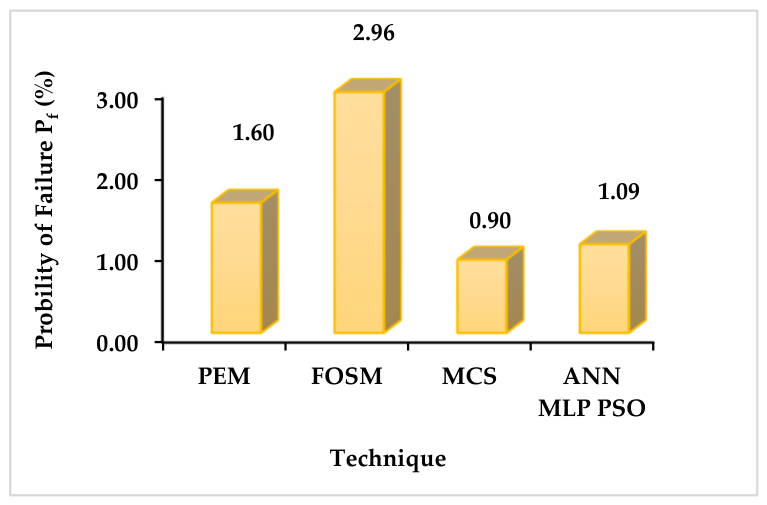
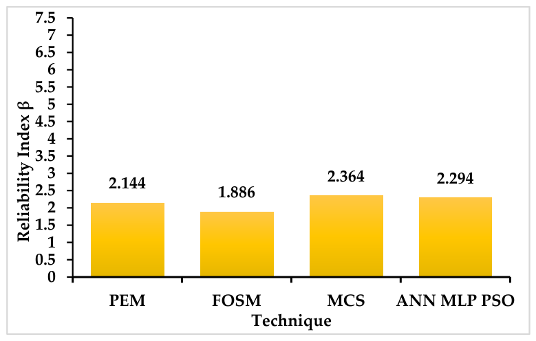
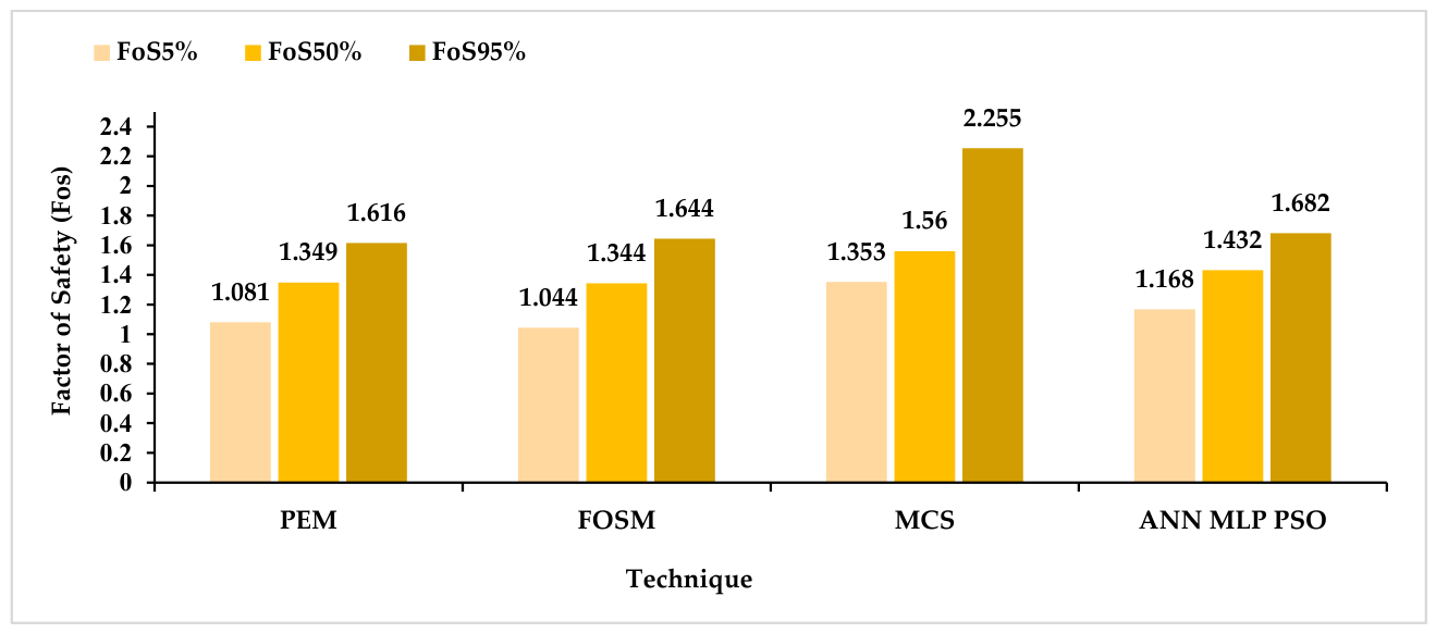
Absolute ANN–MCS deviation	0.238	0.130	6.22	0.070	0.19	0.185	0.128	0.573

reports the reliability results for the dry condition obtained using four probabilistic frameworks: MCS, FOSM, PEM, and ANN–MLP–PSO surrogate sampling. For the same dry scenario, Figure 13, Figure 14 and Figure 15 provide a direct graphical comparison of the corresponding outputs across the four approaches. Figure 13 reports the probability of failure, Pf. Figure 14 presents the reliability index, β. Figure 15 presents the FoS quantiles (5%, 50%, and 95%). Together, these figures facilitate a direct comparison of method-to-method differences under dry conditions.

Under dry conditions, the four probabilistic approaches produced generally consistent reliability assessments, indicating a stable slope condition with relatively low probabilities of failure. Although differences were observed in the predicted reliability metrics and FoS distribution characteristics, all methods yielded results within the same overall stability regime. These variations are attributable to the different mathematical formulations underlying the investigated approaches. MCS relies on direct probabilistic sampling, FOSM employs first-order moment approximations, PEM uses discrete point-estimate representations, and ANN–MLP–PSO approximates the slope stability response through a data-driven surrogate model. Consequently, differences in probabilistic representation, response-surface nonlinearity, and approximation assumptions may lead to variations in the predicted reliability indicators even when identical input distributions and limit-state definitions are adopted.

Furthermore, the reliability metrics were computed using different estimation procedures. For the sampling-based approaches (MCS and ANN probabilistic propagation), the probability of failure (P_f) was obtained directly from the proportion of realizations satisfying FoS < 1, and the corresponding reliability index (β) was subsequently derived from P_f. In contrast, FOSM and PEM estimate β from the first two moments of the FoS distribution under an approximate normality assumption, from which P_f is then calculated. Therefore, exact numerical agreement among the investigated reliability methods should not necessarily be expected, particularly for nonlinear slope stability problems characterized by asymmetric probabilistic response behavior. Nevertheless, all four approaches were implemented using the same deterministic slope geometry, identical probabilistic characterization of the uncertain variables (c, ϕ, γ, R_u), the same limit-state definition g(X) = FoS(X)−1, and consistent Morgenstern–Price slope stability assumptions, thereby enabling a direct and fair comparison of the resulting reliability predictions.

Table 8. Wet case probabilistic reliability outputs and FoS quantiles.

Technique	Mean FoS μ	Std. Dev. FoS σ	COV (%)	Reliability Index β	Pf (%)	FoS5%	FoS50%	FoS95%
PEM	0.776	0.185	23.80	−1.211	88.70	0.472	0.776	1.080
FOSM	0.793	0.137	17.30	−1.510	93.40	0.567	0.793	1.019
MCS	0.626	0.164	26.20	−2.290	98.90	0.424	0.591	0.947
ANN–MLP–PSO	0.764	0.191	25.04	−1.082	86.03	0.502	0.735	1.112
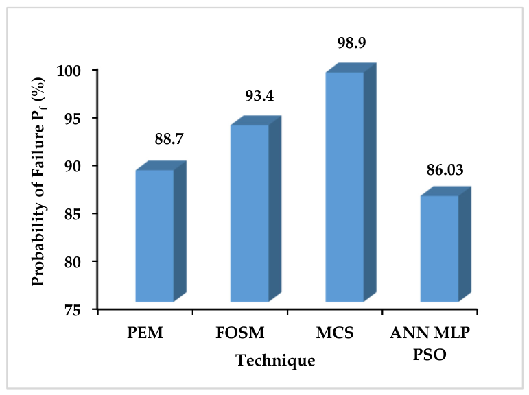
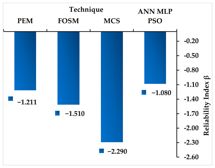
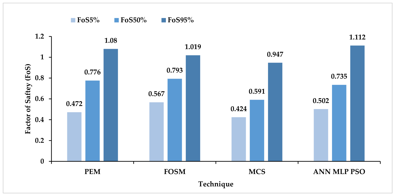
Absolute ANN–MCS deviation	0.138	0.027	1.16	1.208	12.87	0.078	0.144	0.165

reports the probabilistic reliability outputs obtained under wet conditions, where R_u is modeled as a random variable according to the probabilistic characterization defined in the case study section. The corresponding graphical comparisons of probability of failure (Pf), reliability index (β), and FoS quantiles are presented in Figure 16, Figure 17 and Figure 18, respectively.

Under wet conditions, all four probabilistic approaches predicted a pronounced deterioration in slope reliability relative to the dry condition, indicating a transition toward highly unstable behavior. Although quantitative differences were observed among the predicted reliability metrics, the investigated methods consistently identified the same overall hydraulic reliability trend, namely a substantial reduction in FoS and a marked increase in the probability of failure associated with elevated pore-water pressure conditions. The observed differences are attributable to the distinct mathematical formulations of the reliability approaches, including direct probabilistic sampling (MCS), moment-based approximation (FOSM), point-estimate representation (PEM), and surrogate-based prediction (ANN–MLP–PSO). Nevertheless, all methods provided a consistent engineering interpretation of the wet-condition response under the prescribed hydraulic model.

4.3. Height-Domain Robustness Assessment

To assess whether the wide global height range influenced the Mansourieh application, an auxiliary ANN–MLP model was developed using only database cases satisfying 10 ≤ H ≤ 50 m. The resulting locally relevant subset contained 1326 cases. The original global train–test membership was preserved: 1070 cases belonged to the training partition and 256 cases belonged to the independent held-out testing partition. Consequently, no locally relevant test case was used during restricted-model training.

To isolate the influence of the training-height domain, the PSO-selected architecture [72,75,77,80,81] was retained without performing a new architecture search. The activation pattern, loss function, reliability-oriented sample weighting, Adam optimizer settings, dropout rate of 0.1, L2 coefficient of 0.001, batch size of 32, and final training duration of 400 epochs were also retained. A separate z-score scaler was fitted exclusively to the 1070 restricted training cases and was subsequently applied without modification to the 256 restricted test cases. Thus, the principal difference between the global and restricted models was the height domain used for model training. The restricted model achieved R² = 0.935, RMSE = 0.239, MAE = 0.151, and a mean prediction bias of −0.091 on the 256 independent locally relevant test cases. These results demonstrate that the fixed ANN architecture maintained strong predictive performance when trained and evaluated using slopes within the height interval containing Mansourieh.

The Mansourieh probabilistic assessment was subsequently repeated using the restricted surrogate and the same case definition adopted in the original analysis: H = 24 m, θ = 29°, lognormally distributed cohesion with μ_c = 4.0 kPa and COV = 50%, normally distributed friction angle with μ = 30° and σ = 3°, normally distributed unit weight with μ_γ = 18.5 kN/m³ and σ = 1.3 kN/m³, R_u = 0 for the dry condition, and R_u ∼ Triangular (0.20, 0.40, 0.55) for the wet condition (

Table 9. Sensitivity of the Mansourieh ANN–MLP–PSO reliability results to the training-height domain.

ANN Training Domain	Mean FoS μ	Std. Dev. FoS σ	COV (%)	Reliability Index β	Pf (%)	FoS5%	FoS50%	FoS95%
Global-Dry (1.10 ≤ H ≤ 511) m	1.433	0.154	10.76	2.294	1.09	1.168	1.432	1.682
Restricted-Dry (10 ≤ H ≤ 50) m	1.317	0.172	13.08	1.710	4.36	1.011	1.335	1.585
Global-Wet (1.10 ≤ H ≤ 511) m	0.764	0.191	25.04	−1.082	86.03	0.502	0.735	1.112
Restricted-Wet (10 ≤ H ≤ 50) m	0.735	0.152	20.66	−1.682	95.38	0.505	0.732	0.992

The global-model values are the ANN–MLP–PSO results originally reported in Table 7 and Table 8. The restricted-model values were obtained from the auxiliary height-domain analysis. The comparison evaluates the sensitivity of the reported reliability summaries to the ANN training-height domain.

). A total of 20,000 ANN-based probabilistic realizations were evaluated for each hydraulic condition.

Restricting the training-height domain produced more conservative reliability estimates for both hydraulic conditions. Under dry conditions, the mean FoS decreased from 1.433 to 1.317, while the estimated probability of failure increased from 1.09% to 4.36%. Nevertheless, both models retained a mean FoS above unity, a positive reliability index, and a comparatively low failure probability. Under wet conditions, the mean FoS changed from 0.764 to 0.735 and the probability of failure increased from 86.03% to 95.38%. Both models therefore identified a failure-dominated wet-condition response, with a mean FoS below unity and a negative reliability index.

The numerical changes demonstrate that the site-specific reliability estimates are sensitive to the height composition of the ANN training database. Accordingly, inclusion within the global applicability bounds should not be interpreted as numerical invariance with respect to training-domain selection. However, the principal engineering interpretation remained unchanged: both training domains predicted a generally stable dry-condition response and a pronounced transition to a failure-dominated response under the prescribed wet hydraulic scenario. The restricted model therefore provides a locally focused robustness assessment that supports the consistency of the ANN reliability classification across the two prescribed hydraulic scenarios.

5. Discussion

The dry-to-wet comparison was used to assess the ability of the ANN–MLP–PSO surrogate to reproduce the reliability response obtained from FOSM, PEM, and MCS under identical probabilistic input models and the same limit-state definition. Under dry conditions (R_u = 0), variability in the soil-strength parameters did not shift a substantial portion of the FoS distribution below unity, and the estimated probabilities of failure remained low. Under the prescribed wet scenario, the increase in pore-water pressure reduced the calculated FoS across all methods, with mean values ranging from 0.626 to 0.793, negative reliability indices, and failure probabilities between approximately 86% and 99%. These numerical results demonstrate that the surrogate captured the same change in reliability regime identified by the conventional methods, while the remaining differences reflect the distinct response-evaluation and uncertainty-propagation procedures adopted by each technique.

Relative to the dry case, all methods predict substantial reductions in mean FoS, the appearance of negative reliability indices, and marked increases in failure probability, indicating a transition from a generally stable condition to a failure-dominated regime. As an illustrative example, the FOSM results show a reduction in mean FoS from 1.344 under dry conditions to 0.793 under wet conditions, accompanied by a shift in reliability index from β = 1.886 to β = −1.510 and an increase in failure probability from 2.96% to 93.40%. The corresponding FoS quantiles further indicate that even statistically favorable realizations remain only marginally stable under saturated conditions. Collectively, the dry-to-wet comparison shows that all four methods produced consistent changes in the mean FoS, distributional spread, reliability index, and probability of failure under the adopted hydraulic input models. The agreement in reliability regime provides the principal basis for evaluating the probabilistic performance of the ANN–MLP–PSO surrogate.

The observed differences among the probabilistic methods are primarily attributable to their distinct mathematical formulations and their treatment of nonlinearity near the limit state. MCS propagates uncertainty through direct probabilistic sampling and repeated deterministic evaluations, whereas FOSM relies on first-order linearization about the mean input point and PEM estimates response statistics using a limited number of representative point evaluations. The higher mean FoS obtained from MCS under dry conditions (μ = 1.671), relative to FOSM and PEM (μ ≈ 1.34), reflects the right-skewed lognormal cohesion distribution (COV = 50%). MCS samples the full upper tail of the resulting FoS response, whereas FOSM evaluates the response only at the mean input vector and PEM uses symmetric point estimates—neither of which captures this skew. The four methods nonetheless agree on a low probability of failure and a stable dry-condition regime. Consequently, each method captures nonlinear response behavior and distribution-tail characteristics to a different extent. These methodological differences become more pronounced under wet conditions, where elevated pore-water pressures increase the sensitivity of the reliability response to small changes in the governing variables. Despite these methodological differences, FOSM, PEM, and MCS establish a consistent benchmark reliability regime against which the ANN–MLP–PSO results can be evaluated under the prescribed wet hydraulic scenario. The quantitative comparison reported in Table 7 and Table 8 characterizes the numerical deviations between ANN–MLP–PSO and MCS under the dry and wet scenarios.

Under the dry condition, the reliability index and probability of failure exhibit small absolute deviations of 0.070 and 0.19 percentage points, respectively. The largest difference occurs in the 95th-percentile FoS, with an absolute deviation of 0.573, accompanied by a difference of 0.130 in the FoS standard deviation. These results indicate that ANN–MLP–PSO and MCS provide closely comparable failure indicators under the dry condition, despite differences in the dispersion and upper range of their FoS distributions.

Under the wet scenario, the absolute deviations in the mean and median FoS are 0.138 and 0.144, respectively. ANN–MLP–PSO produces a higher mean and median FoS than MCS and consequently yields a probability of failure that is 12.87 percentage points lower and a reliability index differing by 1.208. Nevertheless, both approaches identify a failure-dominated response under the wet scenario. The resulting probabilities are conditional on the prescribed R_u distribution and should not be interpreted as estimates of the current or annual field probability of failure.

The numerical deviations between the two approaches can be attributed to differences in response evaluation and probabilistic sampling. Direct MCS evaluates the deterministic Morgenstern–Price slope stability model for each realization, whereas ANN–MLP–PSO propagates the sampled inputs through the trained surrogate. Furthermore, although both analyses adopt the same prescribed probability distributions and a sample size of 20,000 realizations, their random input samples are generated independently rather than shared realization by realization. Consequently, the resulting empirical moments, FoS quantiles, and failure counts are not expected to be numerically identical. The observed deviations therefore reflect the combined influence of the different response-evaluation mechanisms and independent finite samples.

Differences in the location and dispersion of the resulting FoS distributions subsequently propagate into the calculated reliability indicators. The probability of failure is determined from the proportion of realizations satisfying FoS < 1, while the reliability index is derived from the corresponding failure probability. Consequently, the observed differences in mean FoS, standard deviation, and FoS quantiles lead to corresponding differences in P_f and β. The comparison demonstrates consistency in the overall engineering interpretation while identifying the magnitude and methodological basis of the numerical deviations between ANN–MLP–PSO and direct MCS.

The predicted reliability metrics fall within the range established by the benchmark methods and remain particularly close to the PEM and FOSM estimates, while preserving the overall reliability trends identified by the simulation-based MCS approach. These observations indicate that the ANN surrogate successfully reproduces the principal probabilistic response characteristics of the slope system and provides reliability assessments that are consistent with those obtained from conventional probabilistic techniques.

From a computational perspective, the ANN-based reliability workflow combines probabilistic sampling with surrogate-based response evaluation, replacing repeated deterministic slope stability analyses with rapid ANN inference once the model has been trained. This substitution yields substantial computational efficiency gains while retaining reliability trends that are consistent with those obtained from the benchmark probabilistic approaches. A deterministic behavioral check showed a monotonic reduction in predicted FoS with increasing R_u, consistent with the expected hydraulic response of a slope. This check evaluates the plausibility of the predicted trend but does not introduce a governing-equation constraint into the data-driven surrogate.

Overall, the results demonstrate that ANN–MLP–PSO reproduced the dry-to-wet changes in probabilistic reliability metrics obtained from FOSM, PEM, and MCS under identical input distributions and the same limit-state definition, while providing an efficient surrogate framework for probabilistic slope stability assessment.

The height-domain robustness assessment provides an additional qualification of the global-model findings. Although the restricted surrogate produced more conservative numerical reliability estimates than the original global surrogate, it reproduced the same dry-to-wet stability transition. The dry-condition mean FoS remained above unity and the corresponding probability of failure remained below 5%, whereas the wet-condition mean FoS remained below unity and the probability of failure exceeded 95%. Thus, the qualitative engineering conclusion was robust to restriction of the training-height domain, while the differences in the numerical reliability indicators demonstrate that site-specific point estimates remain sensitive to training-data composition.

6. Limitations and Future Work

Despite the encouraging performance of the proposed ANN–MLP–PSO framework, several limitations should be acknowledged. First, the surrogate remains dependent on the representativeness and composition of its training database. Although the global database spans broad geometric, geotechnical, and hydraulic ranges, the height-domain robustness analysis demonstrated that numerical site-specific reliability estimates can vary when the training data are restricted to slopes physically closer to the application case, even when the case lies within the global input bounds. Therefore, range inclusion should not be interpreted as guaranteeing numerical invariance or complete local validity. The restricted analysis nevertheless reproduced the same reliability classification under both prescribed hydraulic scenarios, indicating that the qualitative interpretation was not controlled by the sparsely populated extreme-height tail.

Second, the present study is restricted to homogeneous soil slopes and therefore does not explicitly account for layered stratigraphy, spatially variable material properties, anisotropic soil behavior, or progressive failure mechanisms. While this assumption enables a controlled comparison between the investigated probabilistic approaches, additional complexities may influence reliability behavior in real geotechnical systems.

Third, wet hydraulic conditions were represented through the pore-water pressure ratio (R_u) rather than a fully coupled transient seepage analysis. This simplified representation was adopted to ensure methodological consistency among ANN–MLP–PSO, MCS, FOSM, and PEM within a unified probabilistic framework. Consequently, the reported wet-condition results should be interpreted as reliability estimates associated with generalized hydraulic degradation rather than site-specific transient infiltration processes.

Finally, the ANN surrogate was treated deterministically during probabilistic propagation, and uncertainty associated with model-form approximation, training variability, and extrapolation beyond the training domain was not explicitly propagated into the reported reliability metrics.

Future research should focus on extending the proposed framework to more complex geotechnical conditions, including heterogeneous and layered slopes, spatially variable material properties, and rainfall-induced transient seepage scenarios. Additional validation using independent field case studies and broader geological settings would further strengthen assessment of the framework’s generalizability and practical applicability.

7. Conclusions

This study developed a reliability-oriented ANN–MLP–PSO framework for probabilistic slope stability assessment and benchmarked its performance against three established reliability approaches, namely the First-Order Second-Moment method (FOSM), the Point Estimate Method (PEM), and Monte Carlo simulation (MCS). Unlike conventional ANN applications that focus primarily on deterministic factor-of-safety prediction, the proposed framework extends ANN-based modeling to probabilistic reliability evaluation through surrogate-based uncertainty propagation, enabling estimation of probability of failure (Pf), reliability index (β), and FoS distribution characteristics under a unified reliability framework. Under dry conditions, all methods predicted generally stable behavior characterized by FoS distributions centered above unity, positive reliability indices, and low probabilities of failure. In contrast, wet conditions produced a substantial deterioration in reliability, reflected by mean FoS values below unity, negative reliability indices, and failure probabilities ranging from approximately 86% to 99%.

Although quantitative differences were observed among the investigated reliability approaches, FOSM, PEM, MCS, and ANN–MLP–PSO consistently identified the same overall reliability trends and engineering interpretation. The ANN surrogate produced reliability metrics that remained consistent with the range established by the benchmark methods and successfully reproduced the principal probabilistic response characteristics of the slope system. These results demonstrate that the ANN–MLP–PSO model can be used as a data-driven FoS surrogate within a probabilistic reliability framework. An auxiliary height-domain assessment further examined the applicability of the surrogate to the 24 m Mansourieh slope. Restricting model training to 10 ≤ H ≤ 50 m produced more conservative numerical reliability estimates but retained the same engineering interpretation: the dry condition remained characterized by a mean FoS above unity and comparatively low failure probability, whereas the wet condition remained failure-dominated, with a mean FoS below unity and P_f > 95%. This result demonstrates that the reliability classification remained consistent across the two training-height domains, while the quantitative site-specific reliability estimates remained sensitive to the composition of the training database.

From a practical perspective, the proposed framework enables rapid probabilistic evaluation once the surrogate has been trained, eliminating the need for repeated deterministic slope stability analyses during uncertainty propagation. The combination of computational efficiency and consistency with the benchmark reliability results supports the use of ANN–MLP–PSO as a tool for reliability-oriented geotechnical assessment, probabilistic screening, and comparative reliability analysis under uncertainty.