
Article

Uncertainties of Estimating the Conductive Heat Flux at a Pavement Surface

1
School of Intelligent Construction, Guangxi Minzu University, 188 University Road, Nanning 530006, China
2
Engineering Operation and Maintenance Intelligent Monitoring and Testing Research Center of Engineering Technology, Guangxi Minzu University, 188 University Road, Nanning 530006, China
3
School of Civil and Environmental Engineering, University of Technology Sydney, 15 Broadway, Ultimo, NSW 2007, Australia
*
Author to whom correspondence should be addressed.
Infrastructures 2026, 11(7), 216; https://doi.org/10.3390/infrastructures11070216
Submission received: 19 May 2026 / Revised: 8 June 2026 / Accepted: 17 June 2026 / Published: 24 June 2026
(This article belongs to the Special Issue Sustainable Road Infrastructure: Safety, Performance and Resilience)

Abstract

Conductive heat flux (G) at pavement surfaces plays a vital role in managing internal temperature variations. G can be calculated either as the residual of solar absorption, heat convection, and long-wave radiation, or as the product of thermal conductivity and the temperature gradient near the surface. Both methods, however, are subject to uncertainties due to measurement parameters. For the two methods, this study formulates the uncertainty of the conductive heat flux at the pavement surface. The experiment was designed to measure pavement interior temperatures and external weather data so that the uncertainties of the two methods can be quantified and compared. It was found that ΔG estimated by the residual method is significantly higher than that calculated using conductivity and temperature gradient. The key factors influencing ΔG in the residual method, in order, are wind speed, incident solar radiation, and reflectivity, with other factors such as surface and air temperatures, relative humidity, and emissivity having minimal impact. In contrast, the primary contributors to ΔG in the conductivity and temperature gradient method are the temperature gradient and thermal conductivity. The residual method is crucial for predicting pavement temperatures when no pre-installed temperature sensors are available, and enhancing wind speed measurement precision can significantly reduce the uncertainty of G. The study finds that the approach of estimating G through conductivity and temperature gradient showed lower uncertainty than the residual method, particularly in complex urban environments.

1. Introduction

Understanding pavement temperature is pivotal for elucidating the thermal dynamics of pavements and comprehending the heat partitioning at their surfaces. One method to grasp this phenomenon involves embedding temperature sensors within the pavement to log temperatures at different depths. However, this approach is often costly and time-consuming, particularly for existing pavements, as it requires the demolition and subsequent rehabilitation of the pavement surface for sensor installation. An alternative strategy is the numerical or analytical resolution of the pavement’s heat flow, which can yield insights into the temperature variation at various depths. This method hinges on the precise calculation of heat fluxes entering and exiting the pavement. Given that pavements exhibit significant temperature fluctuations near the surface and minimal changes at the bottom, accurately estimating the conductive heat flux at the pavement surface is crucial for reliable pavement temperature predictions. At the pavement surface, the heat flux process is complex, involving incident and reflected solar radiation, heat convection, and long-wave radiation. The residual of these components constitutes the conductive heat flux into the pavement. The scenario alters at night, as the heat stored in the pavement during the day is released, sustaining heat convection and long-wave radiation at the surface. Consequently, the conductive heat flux at the pavement surface becomes a critical component of the pavement’s overall heat balance and dynamically varies throughout the day. This intricate interplay of various thermal processes underlines the need for comprehensive and nuanced approaches to accurately model and predict pavement temperatures, a key aspect in understanding urban heat dynamics and pavement material performance.
The residual method is extensively utilized to determine the conductive heat flux to pavements. Initially, Oke and Cleugh [1] outlined a method for estimating heat storage in urban environments, focusing on a suburban area in Vancouver. The approach, known as the residual method, involves calculating the conductive heat flux in pavements. This flux is derived from the energy balance equation’s residual, considering variables like net all-wave radiation flux, anthropogenic heat flux, and turbulent flux densities of sensible and latent heat. The net heat storage term accounts for total heat uptake or release from the urban system, including changes in air, buildings, vegetation, and ground. Later, Asaeda and Ca calculated this conductive heat flux at the pavement-air interface [2]. Their findings indicate that the instantaneous conductive heat flux of pavement can range between −100 and 200 W/m2, with asphalt pavements exhibiting higher fluxes. This residual conductive heat flux, crucial for modeling pavement temperature, is typically defined as the heat flux at the upper boundary [3,4]. Recently, numerical models have frequently utilized the residual method to estimate upper boundary heat flux in simulations of pavement temperature fluctuations [5,6,7], although details of conductive heat flux calculation may be different. However, this methodology is accompanied by notable uncertainties due to the error propagation from each variable—heat convection, solar radiation, and reflectivity, each beset with measurement inaccuracies. Additionally, the uncertainty in long-wave radiation, stemming from the difficulty in accurately measuring pavement and sky emissivity and sky temperature, further complicates the assessment. These uncertainties collectively impact the conductive heat flux estimation, making the quantification of this uncertainty vital for evaluating the reliability of predictive models in this domain. This cumulative uncertainty arises from many measurement parameters such as wind speed, solar radiation, air temperature, etc., as well as from the model to compute the conductive heat flux; however, remained unreported and unknown.
This research investigates the uncertainties in measuring conductive heat flux on pavement surfaces, with a particular focus on the residual method and factors contributing to its overall uncertainty. The study also explores uncertainties in conductive heat flux calculations derived from the combination of pavement thermal conductivity and surface temperature gradient. To quantify these uncertainties, an experiment was conducted, gathering pavement temperature and weather data in the field. The study includes a comparative analysis of both methods, emphasizing the identification and prioritization of the main factors contributing to uncertainty in each method.

2. Methodology

2.1. Theoretical Model for ΔG of the Residual Method

Incident solar radiation, denoted as I, is primarily absorbed by the pavement surface with a solar absorption factor of (1 − r), where r represents the reflectivity of the pavement. This solar absorption is drained through heat convection (H) and net longwave radiation (L). The residual heat flux is conductive heat flux (G), that is
G   = ( 1 r ) I H L
where the negative sign means the heat flux leaving the pavement surface. In Equation (1),
H =   h c ( T s T a )
where Ts (°C) represents the pavement surface temperature and Ta (°C) is the air temperature, and hc (W/m2∙°C) is the heat convection coefficient. In this study, an empirical formulation widely used in pavement-temperature modelling was adopted because it provides sufficient accuracy and requires wind speed as the main input for estimating hc [8]:
h c   =   { 5.6   +   4.0 v v   <   5 7.2   ×   v 0.78 v     5
where v (m/s) is the wind speed measured at a height of 9.0 m. For the relatively open experimental site considered in this study, wind speed (vm) measured at a different height (zm) above the pavement surface was converted to that at the reference height by [9]:
v   =   v m ( 9 / z m ) 1 7
Here, the wind speed (vm) was observed at a height of zm.
In Equation (1), L includes the incident longwave radiation and the outgoing longwave radiation (from the pavement), as expressed as
L   = e σ ( ( T s + 273.15 ) 4 ( T y + 273.15 ) 4 )
where Ty = sky temperature and e = emissivity of the pavement and σ = 5.67 × 10⁻⁸ Wm−2K−4.
Equation (5) is relatively complex and complicates the analysis of L, Ts, and Ty. It can be simplified using a first-order approximation of the Maclaurin series expansion, balancing computational efficiency with maintained accuracy [10].
L = 4.62 e ( T s T y )
For the sky temperature, it can be found by
T y = e y 0.25 ( T a + 273.15 ) 273.15
And ey is the emissivity of the sky
e y = 0.754 + 0.0044 T d
where Td (°C) is dew point:
T d   =   b γ / ( a γ )
where a = 17.3, b = 237.7, and γ   =   a T a / ( b   +   T a )   +   ln ( θ / 100 ) (here Ta in °C) [11].
According to Equations (1)–(8), the conductive heat flux G can be expressed as a function of
G = G ( T a ,   T s ,   v ,   θ ,   r ,   I ,   e )
The uncertainty in conductive heat flux ΔG can be calculated using the root sum square of the product of the partial derivatives of G with respect to each variable. Equation (11) is the explicit formula for considering each of the variables and their respective uncertainties:
Δ G   = ( G T a Δ T a ) 2 + ( G T s Δ T s ) 2 + ( G v Δ v ) 2 + ( G θ Δ θ ) 2 + ( G r Δ r ) 2 + ( G I Δ I ) 2 + ( G e Δ e ) 2
The corresponding partial derivatives are:
G T a   =   h c 4.62 e   ×   e y 0.25
G T s   = h c 4.62 e
G v = ( T s T a ) h c v
h c v = 4   ( v   <   5 )   and = 7.2   ×   0.78   ×   v 0.22   ( v     5 )
G θ = 4.62 e   ×   0.0044   ×   0.25   ×   e y 0.75   ×   ( T y + 273.15 )   ×   T y ab ( a γ ) 2 1 θ
G r = I
G I = 1 r
G e = 4.62 ( T s T y )
According to Equation (11), the uncertainty of G is dependent on serially measured parameters, including the air temperature (Ta), surface temperature (Ts), wind speed (v), relative humidity (θ), incoming solar radiation (I), surface reflectivity (r), and the emissivity (e). Once the measurement uncertainty of each instrument is known, cumulative uncertainty ΔG is appraised.

2.2. Theoretical Model for ΔG Based on a Surface-Centered Polynomial Approximation of T(z)

As an alternative to the residual model, the G value of a pavement can be calculated by using the Fourier Law of heat conduction, that is
G = k T z / z = 0
where k (W/m·K) is the thermal conductivity of the pavement surface layer, which can be regarded as a constant, typically with a value of 0.8 to 2.5. With the k value known, G can be calculated if the temperature T(z) in the entire pavement is known, so the derivative of ∂T/∂z(z = 0) is estimated. In this study, G is defined as positive when heat is transferred into the pavement.
At a given time (t), heat transfer within the homogeneous pavement surface layer is assumed to be dominated by one-dimensional transient conduction. This assumption is reasonable because the measurement location was far from pavement edges and surrounding structures, and the horizontal dimensions of the pavement were much greater than the investigated depth. In the absence of internal heat generation and material interfaces within the investigated depth, the temperature field T(z,t) is expected to vary smoothly with depth near the pavement surface. Therefore, T(z,t) can be locally represented by a truncated Taylor expansion about z = 0:
T ( z , t ) =   T s ( t )   +   T z / z = 0   z +   1 2 2 T z 2 / z = 0 z 2   +   1 6 3 T z 3 / z = 0 z 3 + R 4
where R4 is the remainder term. This expression is not intended to represent a global analytical solution of the transient heat-conduction equation. Instead, it provides a local approximation of the temperature profile near the pavement surface. Centering the expansion at z = 0 is particularly suitable for the present study because the coefficients of the polynomial directly correspond to the physical quantities we need:
a 0   =   T s ( t ) ,   a 1   =   T z | z = 0 ,
Accordingly, the measured temperature profile at each time step was approximated using the following surface-centered polynomial:
T ( z )   =   a 0   +   a 1 z   +   a 2 z 2   +   a 3 z 3
Based on Equations (20), (22) and (23), the uncertainty in ΔG is then calculated by:
Δ G   =   ( G k Δ k ) 2 +   ( G a 1 Δ a 1 ) 2   =   ( a 1 Δ k ) 2   +   ( k Δ a 1 ) 2
In Equation (24), uncertainty in measuring temperature (ΔT) should indeed be included in the calculation of the uncertainty of the heat flux (ΔG). That is, ΔG not only arises from the uncertainty in the thermal conductivity (Δk) but also from the uncertainties in the temperature gradient (Δ(∂T/∂z)), which is directly affected by the uncertainty in temperature measurements (ΔT) and the uncertainty in the depth measurements (Δz).

2.3. Factors to Calculate ΔG

2.3.1. Experiments

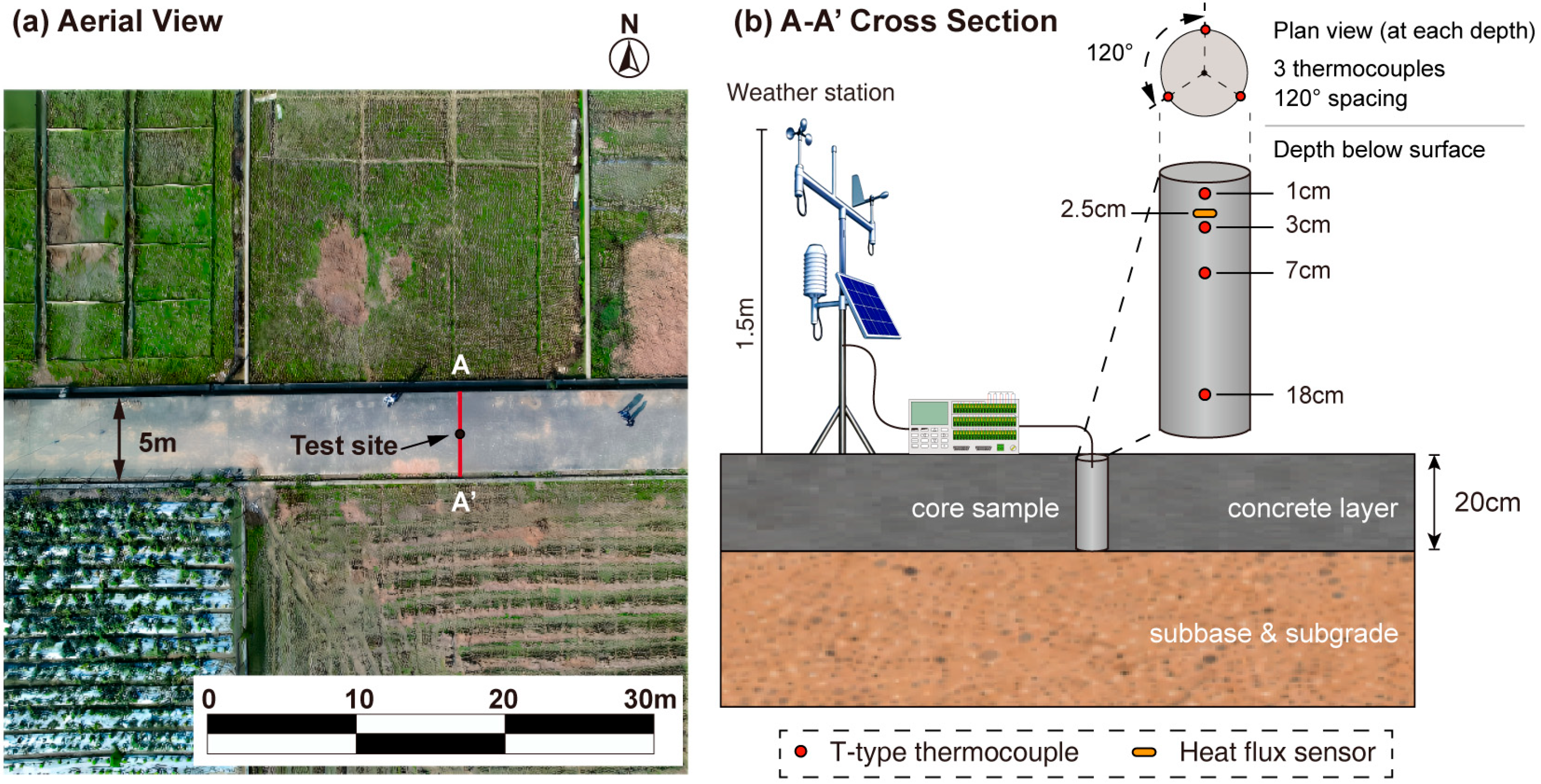
To obtain the temperature profile and weather data of a pavement in the field, an experiment was conducted to observe temperatures at different depths of a pavement and to log the weather information during the experiment. The pavement is a pedestrian-oriented pavement on the Guangxi University campus, occasionally accessed by private cars. This pavement, stretching over 100 m in length and 5 m in width, is depicted in an aerial view in Figure 1a and is oriented east to west. No buildings were located within approximately 100 m of the measurement site, thereby reducing the potential influence of shading and building-induced airflow disturbance. A Davis Vantage Pro2™ Weather Station (Davis Instruments Corporation, Hayward, CA, USA), positioned 1.5 m above the pavement, recorded solar radiation, air temperature, humidity, and wind speed. Table 1 details the station’s precision. Additionally, an albedometer temporarily placed at the road’s center measured the pavement’s reflectivity, yielding an average of 0.225 with a standard deviation of 0.02. However, emissivity was not measured but assumed, with a typical mean value of 0.90 and a standard deviation of 0.01.
To calculate the ΔG derivative using the residual method, surface temperature measurements of the pavement are necessary. However, obtaining these measurements presents challenges. To address this, a 20 cm deep core (matching the surface layer thickness) was drilled in the middle of the pavement. T-type thermocouples were installed at depths of 1 cm, 3 cm, 7 cm, and 18 cm, with three thermocouples at each depth arranged circumferentially 120 degrees apart (Figure 1b). A total of 12 thermocouples were used. After securing the thermocouples, the cored sample was reinserted into its original position, leveled with the surrounding surface, and the gap was filled with cement grout. The surface was finished with grey paste for visual consistency. Data from these sensors were logged every five minutes by a CR3000 datalogger (Campbell Scientific, Logan, UT, USA), concurrently with local weather information, from 2 June 2021 to 25 July 2021. The pavement temperature and weather data recorded during the experiment are provided in Appendix A.
Alongside the weather station and thermal properties, specifying the thermal conductivity (k) and its measurement uncertainty is essential for calculating ΔG in Equation (14). In our experiment, a heat flux sensor was embedded at a depth of 2.5 cm within the core to record the local conductive heat flux. Through regression of the temperature gradient at this depth against the measured heat flux, we determined k to be 1.57 W/m·K with a 6% uncertainty. Consequently, k is assumed to be 0.1 W/m·K (1.57 × 0.06 = 0.094) in this study.

2.3.2. Monte Carlo Simulation

To accurately calculate ΔG, along with the measured weather data and thermal properties such as albedo and emissivity, one must consider the uncertainties of pavement surface temperature (Ts) and of near-surface temperature gradient (a1). Calculating these uncertainties is complex, as they depend on the measurement errors of four temperatures (ΔT) and four depths (Δz). The temperature measurement error for the T-type thermocouple is known to be 0.5 °C. However, the depth z contains uncertainty; for example, a thermocouple intended for a depth of 1.0 cm might actually be at 0.95 cm, 0.98 cm, or another depth. In our experiment, a slot was created to position T-type thermocouples, with three thermocouples duplicated at the same depth.
Consequently, we assumed a depth error (Δz) of 0.1 cm. Using these values (Δz = 0.001 and ΔT = 0.5), a Monte Carlo simulation was performed to determine the uncertainties in Δa1 and ΔTs. The simulation varied Δz and ΔT within their respective ranges randomly and uniformly, recalculating Δa1 and ΔTs for each iteration to assess the stability and reliability of the coefficients. If both Δa1 and ΔTs converged to specific values, these were used to calculate the uncertainties for calculating ΔG. In this study, 1000 Monte Carlo iterations were performed for each temperature profile. In each iteration, the measured temperatures and sensor depths were randomly perturbed within ΔT = ±0.5 °C and Δz = ±0.001 m, respectively. The resulting standard deviations of Ts and a1 were used as ΔTs and Δa1.

3. Results

During our experimental study from 2 June to 30 June, it was observed that the thermocouple temperatures were affected by the cement grout’s hydration process, applied around the core. Then, from 1 July to 16 July, we observed significant effects of intermittent rainfall, notably the evaporation from the wet pavement contributing to the surface heat flux. The data presented in the following section are based on temperature readings and meteorological data collected between 17 July and 25 July.

3.1. Uncertainties of Δa1 and ΔTs

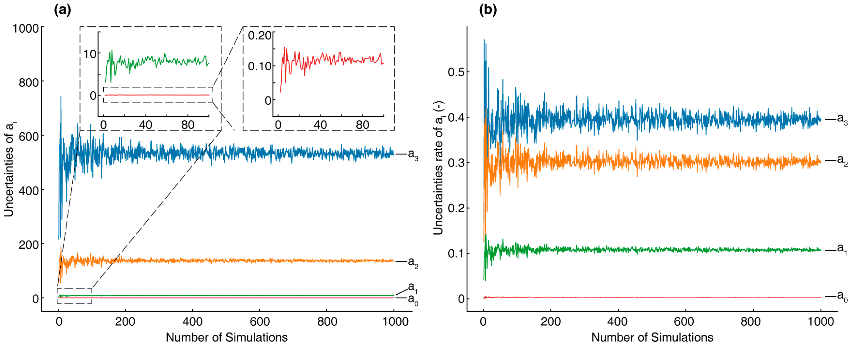
Approximating the pavement temperature profile as the Maclaurin polynomial, convergence of the coefficients is observed with an increase in the number of simulations. Sequentially from the lowest order coefficient, the estimation of Ts (a0) exhibits the smallest uncertainty relative to the higher-order coefficients. Adjacent to Ts is the coefficient a1, which presents a marginally higher uncertainty. The subsequent coefficients, a2 and a3, demonstrate considerably larger uncertainties, reaching approximately 180 and 600, respectively. This elevated uncertainty could be attributed to the fact that the curvature in the T(z) profile is particularly susceptible to perturbations in temperature. The scope of this study does not extend to the detailed examination of the uncertainties associated with a2 and a3.
To scrutinize the values of Ts and a1 more precisely, an inset plot within the main graph has been utilized. This magnified view indicates that post approximately 100 simulations, the uncertainties associated with Ts and a1 approach a state of convergence. The uncertainty of a1 is observed to be within the range of 5–10, and a further focused analysis reveals that the uncertainty in Ts fluctuates around 0.1 °C. Such a discrepancy suggests that the uncertainty inherent in utilizing the regressed temperature profile for determining the surface temperature of pavement is approximately 0.1 °C. Given that the surface temperature can span from 30 to 60 °C, this degree of uncertainty is comparatively insignificant, typically falling below the 1% threshold. Consequently, the ratio of the uncertainty of the coefficient to the coefficient itself, as presented in Figure 2b, is near zero for Ts. In contrast, this ratio for a1 is notably higher, approximately 0.1 (or 10%). This disparity is justifiable, considering that accurately gauging the thermal gradient in proximity to the ground surface poses a significant measurement challenge.

3.2. ΔG Using the Residual Method

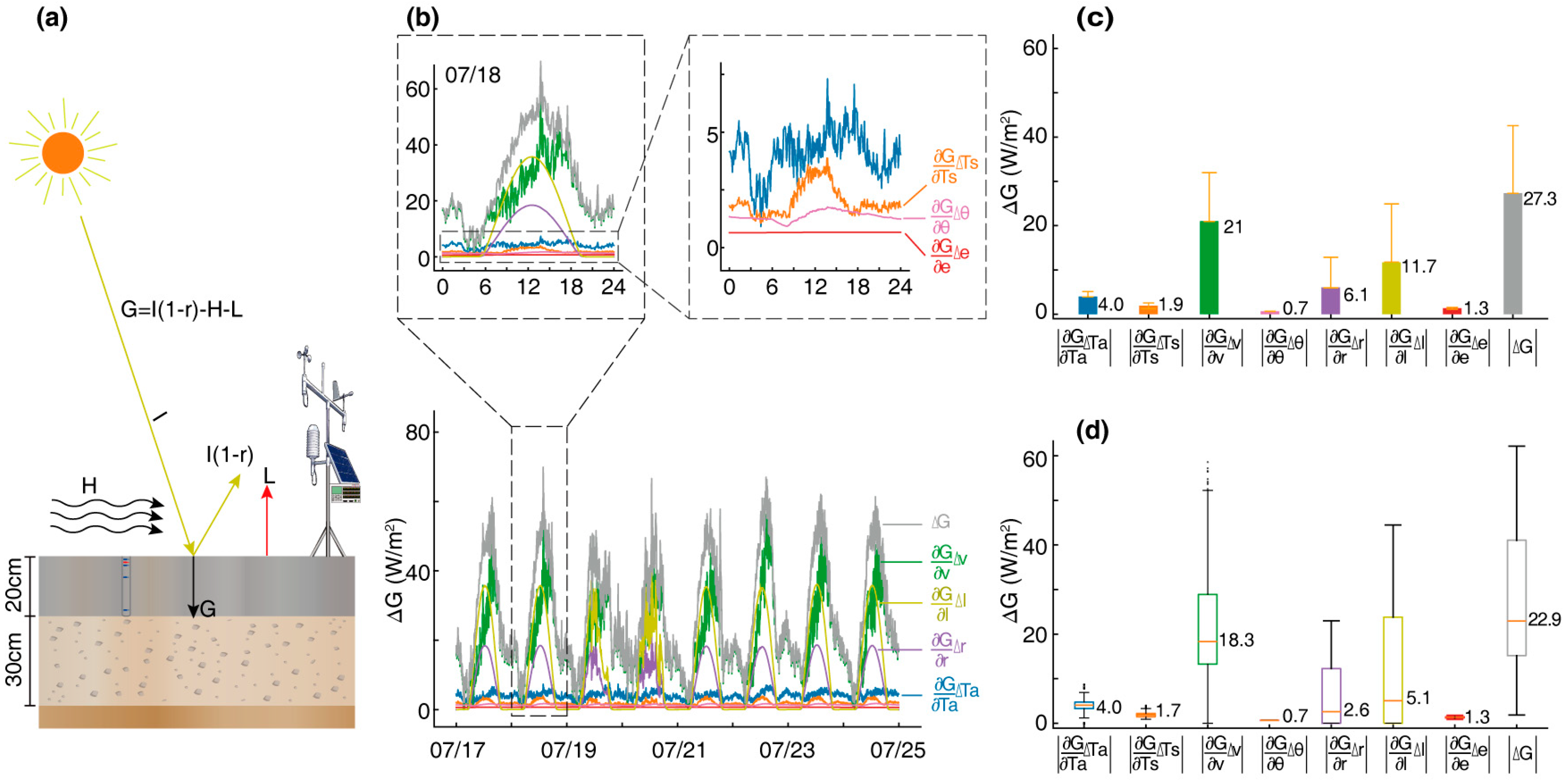
The method for calculating ΔG is detailed in Figure 3a, involving seven variables that influence the uncertainty of the conductive heat flux at the pavement surface. Initially, each variable is isolated to assess its individual impact on ΔG. For example, the influence of air temperature measurement on ΔG is calculated as Δ G   =   G T a Δ T a , while setting the uncertainty of other variables to zero. This approach is repeated for other factors, such as surface temperature, humidity, wind speed, incident radiation, reflectivity, and emissivity. The contribution of each variable to the uncertainty of heat storage at the pavement surface is then plotted. The study culminates in a comparison between the cumulative uncertainty ΔG and the uncertainties contributed by each individual factor.
Figure 3b presents the variation of ΔG from 17 July to 25 July, alongside the uncertainties arising from various contributing factors, denoted as G x Δ x . Notably, while both ΔG and G x Δ x exhibit diurnal fluctuations, their respective patterns diverge owing to the disparate peak values of each factor. Another key observation is the variance in the magnitude of G x Δ x among the factors, some exhibit peak values approaching the cumulative uncertainties ΔG, while others are so minimal that they nearly align with the y = 0 baseline. This discrepancy, particularly in factors such as G T a Δ T a , warrants a more detailed investigation to elucidate their distinct contributions.
The three principal factors contributing to the uncertainty in pavement surface conductive heat flux ΔG were identified as wind speed, incident solar radiation, and measured reflectivity. Contrary to expectations, G I Δ I (pertaining to solar radiation), and G r Δ r (related to reflectivity) do not consistently rank as the top contributors. This observation can be ascribed to the predominant role of solar radiation as the primary driver of temperature variations in pavement surfaces, with solar absorption being a direct function of incident solar radiation (I) and (1 − r). As a result, both G I Δ I and G r Δ r exhibit significant variations. Notably, these factors diminish to negligible levels during nighttime, aligning with the absence of solar absorption. Given a measurement uncertainty of 5% in solar radiation, the uncertainty in I at its peak is approximately 50 W, leading to a corresponding uncertainty range for G I Δ I . As depicted in Figure 3b, on 18 July, G I Δ I is estimated to be around 38 W. Surprisingly, G v Δ v , representing wind speed, emerges as the predominant factor, surpassing others in both day and night values. During daytime, particularly from 6:00 AM to 12:00 PM, G v Δ v is observed to be lower due to the dominance of solar radiation and relatively mild wind conditions. However, outside this period, G v Δ v assumes dominance, peaking between 15:00 and 18:00. Post 18:00 until 6:00 the next day, the contribution of G v Δ v aligns closely with ΔG, indicating that during these hours, the influence of other factors on ΔG becomes insignificantly small compared to the impact of G v Δ v .
Two additional factors contributing to ΔG, the uncertainty in conductive heat flux at the pavement surface, are identified as air-temperature related ( G T a Δ T a ) and surface-temperature related ( G T s Δ T s ) uncertainties. Given the close association of conductive heat flux with both air and surface temperatures, one might anticipate these factors to significantly influence the total uncertainty in ΔG, as minor variations in G could lead to substantial fluctuations in Ts. However, on 18 July, the uncertainty attributed to these factors was observed to be less than 7.5 W, markedly lower than uncertainties induced by wind speed, incident solar radiation, and reflectivity. The analysis revealed that air-temperature-related uncertainty, G T a Δ T a , does not follow a diurnal pattern, fluctuating around a baseline of 5 W, except between 0:00 and 6:00, where it is relatively lower. In contrast, G T s Δ T s displays a distinct diurnal variation, peaking from 12:00 to 15:00, mirroring the temperature pattern near the pavement surface. Nevertheless, the magnitude of uncertainty associated with air temperature (Ta) is relatively greater than that associated with surface temperature (Ts).
Relative to other factors, the uncertainties associated with emissivity (e) and relative humidity (θ) are markedly smaller, bordering on negligible. Illustrated in Figure 3b, the uncertainty in emissivity, G e Δ e , is confined to less than 2.5 W. Notably, even when the assumed uncertainty for emissivity is augmented from 0.01 to 0.03, its impact on ΔG is found to be minimal. In a similar vein, the uncertainty related to relative humidity, G θ Δ θ , originating from a 3% uncertainty level at the Davis weather station, exerts a minor effect on ΔG. These values, ranging from 0 to 1 W/m2, are so diminutive that they are virtually indiscernible in the graphical representation. The derivation of G θ via the chain rule, while complex, results in a reduced actual uncertainty due to the mitigating effects of this mathematical process. As a consequence, the precision in measuring relative humidity has a trifling impact on accurately determining the conductive heat flux at the pavement surface.
To better grade the contribution of individual uncertainty G x Δ x to the cumulative uncertainty ΔG, we calculated the mean and standard deviation of each individual uncertainty and presented the results in Figure 3c. It is confirmed that G v Δ v and G I Δ I are the top factors contributing to the cumulative uncertainty. The mean uncertainty of G v Δ v is 21 and that of G I Δ I is 11.7. In calculating the cumulative uncertainty, which is the square root of the sum of the squares of individual factors, the contributions of factors with smaller uncertainties tend to be overshadowed by those with larger individual uncertainties. Therefore, it is reasonable that at nighttime, the uncertainty related to wind speed is close to the cumulative uncertainty. The means of uncertainty related to air temperature, surface temperature, relative humidity, and emissivity are 4.0, 1.9, 0.7, and 1.3. The square of these values are 16, 3.8, 0.5, and 1.7, which are approximately two orders of magnitude greater than the square value of G I Δ I (11.72 ≈ 137), and of G v Δ v (212 = 441). Therefore, G v Δ v and G I Δ I are the top factors contributing to the cumulative uncertainty, while other factors contribute less and even negligibly.
We further delineated the contribution of individual uncertainties ( G x Δ x ) to the aggregate uncertainty in pavement-surface conductive heat flux (ΔG) using box plots. This graphical representation reaffirms that the uncertainties arising from wind speed ( G v Δ v ) and incident solar radiation ( G I Δ I ) are predominant in influencing ΔG. However, the insights offered by the box plot extend beyond this initial observation. Firstly, the plot accentuates the more pronounced dominance of G v Δ v , as evidenced by its median value of 18.3 compared to 22.9 for ΔG. Secondly, a common characteristic among most boxes is a skewed distribution, where the median line is located towards the lower quartile. This skewness is attributed to the diurnal pattern of solar radiation, which is null during nighttime and follows a sinusoidal pattern during the day. Thirdly, an intriguing observation is the congruence between the median and mean values for G T a Δ T a , G e Δ e , and G θ Δ θ , all registering at 4.0, 1.3, and 0.7, respectively. This parity suggests that the uncertainties related to air temperature, emissivity, and relative humidity do not exhibit the diurnal variation characteristic of incident radiation.

3.3. ΔG Using the Pavement Temperature Profile T(z)

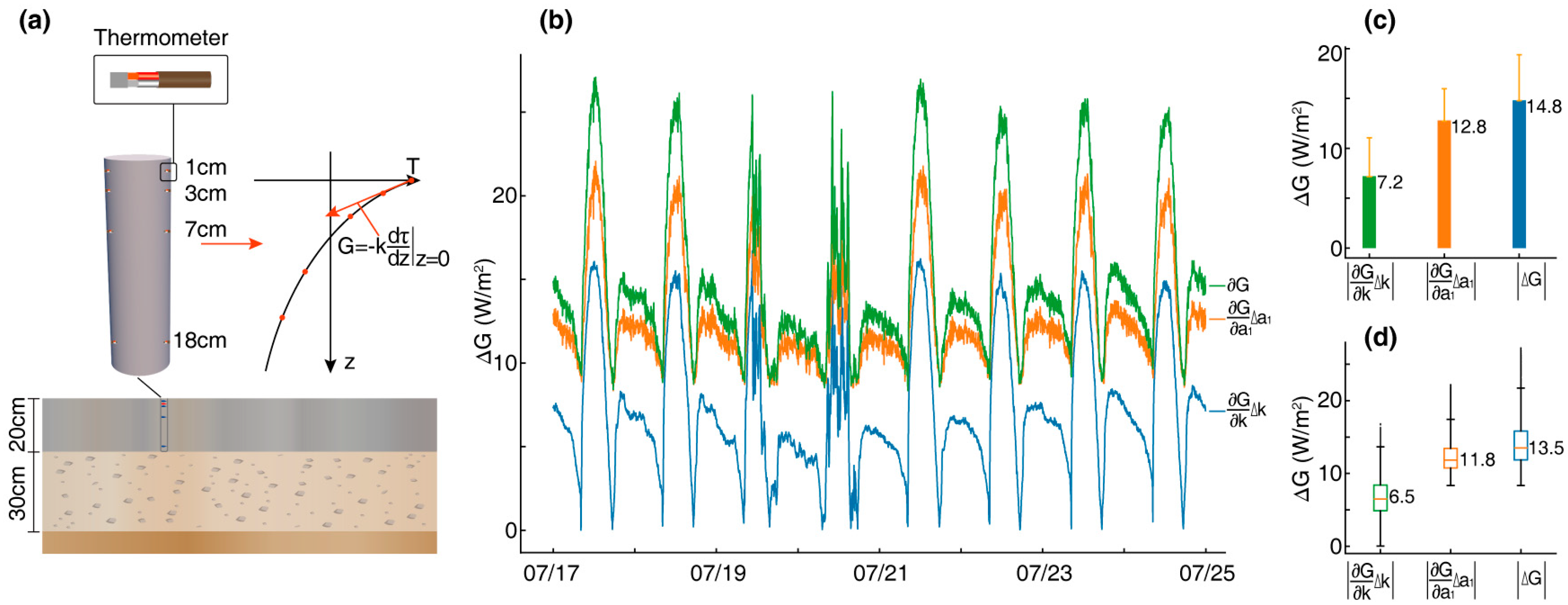
An alternative methodology for estimating ΔG involves employing Equation (10), where the temperature profile of the pavement is derived from logged temperature measurements at various depths, as depicted in Figure 4a. ΔG is subsequently calculated as delineated in Equation (13). Utilizing a1 regressed from the temperature profile and Δa1 as presented in Figure 1a, we obtained the uncertainties G x Δ x and ΔG, which were illustrated in Figure 4b. Within this framework, the primary contributing factors are narrowed down to two: the uncertainty associated with the temperature gradient at pavement surface a1 ( G a 1 Δ a 1 ) and the uncertainty related to thermal conductivity ( G k Δ k ).
Figure 4b presents a comprehensive analysis of the diurnal behavior of the uncertainties in the polynomial coefficients G a 1 Δ a 1 and G k Δ k . A notable observation is that both these uncertainties attain their peak values around solar noon. Specifically, G a 1 Δ a 1 reaches a peak of approximately 20 W/m2, with this value exhibiting day-to-day variability, yet consistently maintaining a minimum threshold around 20 W/m2. Concurrently, G k Δ k consistently peaks at a lower magnitude, around 15 W/m2 each day, and this peak also aligns with solar noon. Despite the daily fluctuations, it is evident that the variations in both G a 1 Δ a 1 and G k Δ k are relatively insensitive to weather changes. Another remarkable pattern is their simultaneous nadir at 8:00 and 15:00. In these instances, G k Δ k exhibits a particularly distinctive behavior, dropping to 0 and then rebounding sharply. This trend suggests that, in the absence of absolute value consideration, G k Δ k may alternate between negative and positive values. This alternating pattern aligns logically with the daytime conductive heat influx into the pavement and the nocturnal heat dissipation from it. Furthermore, the consistent observation that G k Δ k remains below G a 1 Δ a 1 throughout the diurnal cycle is noteworthy. This indicates that, while both factors are significant contributors to the overall uncertainty, G a 1 Δ a 1 dominates in magnitude. The synchronized peaking and troughing of these uncertainties underscore their interrelatedness and the complex dynamics governing the heat storage uncertainties at the pavement surface.
Statistical analysis of the cumulative uncertainty ΔG and its contributing factors substantiates that the uncertainty associated with the temperature gradient near the pavement surface ( G a 1 Δ a 1 ) is the primary contributor to the overall uncertainty. This is further evidenced in Figure 4, where the mean and standard deviation of both G k Δ k and G a 1 Δ a 1 are calculated and presented. The mean values of G k Δ k , G a 1 Δ a 1 , and ΔG are found to be 7.2, 12.8, and 14.8, respectively. The proximity of the mean of G a 1 Δ a 1 to that of ΔG reinforces the notion that temperature gradient uncertainty near the pavement surface is a significant determinant of the cumulative uncertainty. Additionally, a box plot has been generated to illustrate the distribution of G k Δ k , G a 1 Δ a 1 , and ΔG. This plot reveals a slight skew in the distribution of these variables, with median values positioned towards the lower end of the box. Notably, the median of G a 1 Δ a 1 is 11.8, aligning closely with the median of ΔG. This alignment further corroborates the dominant role of G a 1 Δ a 1 in contributing to the cumulative uncertainty in this methodological approach.

4. Discussion

4.1. Implications of the Convective Heat-Transfer Coefficient for Uncertainty Estimation

The primary contributor to the uncertainty in the conductive heat flux (ΔG) is the wind-speed-related term, (∂G/∂v·Δv). This discovery underscores the criticality of enhancing the precision of wind speed measurements to reduce ΔG. The current limitation, however, lies in the precision of our instrumentation, which maintains an accuracy of approximately 5% of the measured value. Thus, improving measurement accuracy is pivotal for bolstering confidence in estimating the conductive heat flux at the pavement surface. Wind speed affects G indirectly through the convective heat-transfer coefficient, hc, and the corresponding convective heat flux, H = hc(TsTa). The wind-speed-related uncertainty depends not only on the magnitude of (Δv), but also on the surface-to-air temperature difference and the sensitivity of the selected hc(v) correlation to wind speed. Therefore, the dominant contribution of wind speed should be interpreted as the combined result of wind-speed measurement uncertainty, the thermal contrast between the pavement surface and the ambient air, and the formulation adopted for hc, rather than as an effect of wind speed alone.
A review of models for estimating the convective heat transfer coefficient, hc, at pavement surfaces, as summarized in Table 2, indicates considerable diversity among existing approaches. The empirical correlations [8,12,13,14,15,16,17,18,19], including the one adopted in this study, estimate hc primarily from wind speed and are therefore simple to apply with routine meteorological data. The Vehrencamp-type models [20,21,22,23,24,25,26,27,28,29,30,31] include both wind speed and the surface-to-air temperature difference, allowing the effects of forced and free convection to be partly represented, but they also introduce additional temperature-dependent uncertainty. The flat-plate models [6,32,33] have a stronger theoretical basis in boundary-layer heat transfer, but require additional parameters such as air thermophysical properties and a characteristic surface length. The Denby model [34,35] is resistance-based and requires aerodynamic resistance, which was unavailable in the present experiment. Therefore, more physically detailed formulations may improve process representation under specific conditions, but they also introduce additional input parameters and potential uncertainty sources. In the absence of independent convective heat-flux measurements, these models listed in Table 2 could not be systematically validated or ranked in this study.
Consequently, this study does not claim that the adopted correlation is universally superior. The reported ΔG quantifies the propagation of measurement uncertainties conditional on the selected hc formulation. Differences among alternative hc correlations constitute model-form uncertainty and were not included in the reported uncertainty values. Similarly, the selection of the long-wave radiation formulation, sky-emissivity model, and wind-speed height-conversion relationship may also introduce model-form uncertainty in the residual method. These model-form uncertainties were not quantified in the present study; therefore, the reported ΔG should be interpreted as the propagated measurement uncertainty conditional on the selected convection and radiation formulations.

4.2. Comparison of the Two Models

The quest to accurately measure the conductive heat flux at the pavement surface (G) has led to a nuanced understanding of the influence of wind speed on this parameter. The residual method, which incorporates wind speed to compute heat convection, adds a significant layer of complexity to this endeavor. This approach, by factoring in the variability of wind conditions, offers a comprehensive method for determining G. Although complex, this method is essential for predicting pavement conditions when pre-buried temperature sensors are not available. The key to enhancing the reliability of our predictions lies in increasing the precision of wind speed measurements, a task that can be challenging due to the dynamic and varied nature of urban landscapes. In urban settings, myriad factors, such as the layout of buildings, vegetation, and topographical features, contribute to a heterogeneity in wind patterns. This variability necessitates localized wind speed measurements, a task complicated by the evolving nature of urban environments and their unique microclimates. As such, while the residual method theoretically allows for accurate G measurements, the practicality of its application across varied and changing urban landscapes remains a significant challenge.
In contrast, estimating G from embedded temperature measurements showed potential for reducing uncertainty compared with the residual method. This method, setting G as the product of a constant (k) and the surface temperature gradient (∂T/∂z at z = 0), demonstrates reduced uncertainty in comparison to methods reliant on external environmental variables such as wind speed. The direct measurement of internal temperature gradients offers a localized and precise assessment of G, effectively circumventing the challenges posed by external factors, including the variability of wind patterns in urban areas. This innovative technique not only enhances the accuracy of estimations of conductive heat flux in pavements but also proves adaptable to the distinctive and variable conditions characteristic of urban environments. As such, this approach to temperature profiling opens new avenues for quantifying heat partitioning on pavement surfaces and could fundamentally transform our understanding of urban heat dynamics. In the pursuit of accurately estimating G through temperature profiles (T(z)), our study finds that increasing the depth and number of temperature measurements within the pavement significantly reduces the uncertainty in G. Currently, we rely on data from four distinct depths, which constrains the accuracy due to the quadratic nature of the Maclaurin polynomial used for analysis. By extending these measurements to include six to ten different depths, particularly in the lower layers of the pavement, we anticipate a marked improvement in the precision of our estimates. This approach would provide a more detailed and reliable data set, enhancing the accuracy of G measurements and reducing the uncertainty associated with our current methodology.

4.3. Limitations and Applicability

Several limitations should be considered when interpreting the results of this study. The field experiment was conducted on one pavement section, and the uncertainty analysis was based on a selected dry-weather period; therefore, the quantitative uncertainty values may vary with pavement materials, surface conditions, climatic regions, and seasonal meteorological conditions. For the residual method, the propagated uncertainty mainly reflects measurement uncertainty under the selected heat-balance formulation, while model uncertainty may also arise from the choice of the convective heat transfer coefficient model, long-wave radiation formulation, and sky-temperature or sky-emissivity parameterization. For the temperature-profile method, the near-surface temperature gradient was estimated from four temperature depths through polynomial fitting and extrapolation, rather than being measured directly; therefore, the reported uncertainty values should be interpreted within the present experimental configuration.
Despite these limitations, the results are useful for engineering situations where pavement conductive heat flux needs to be estimated from either routine meteorological data or embedded temperature measurements. The findings help identify the dominant sources of uncertainty in different estimation methods and provide guidance for selecting an appropriate method under different field-monitoring conditions. Future studies should further examine these conclusions using additional pavement sections, material types, climatic conditions, and denser temperature measurements near the pavement surface.

5. Conclusions

This study delineates two distinct methodologies for estimating the conductive heat flux (G) at pavement surfaces. The first method involves calculating G as the residual of several factors: heat convection, solar radiation absorption, and net long-wave radiation. Alternatively, G can be estimated by embedding temperature sensors within the pavement, logging temperatures at various depths, and considering G as the product of the pavement’s thermal conductivity and the measured thermal gradient at its surface. We formulated, calculated, and compared the uncertainties in heat storage (ΔG) using both approaches. The Monte Carlo simulation was employed to estimate both the thermal gradient at the pavement surface and its surface temperature (Ts), revealing that while Ts has negligible uncertainty, the thermal gradient contains approximately 10% uncertainty. This uncertainty arises from both the precision of the temperature sensors and the ambiguity in their exact depth.
In the residual method, ΔG is influenced by uncertainties in air temperature, surface temperature, wind speed, relative humidity, incident radiation, reflectivity, and emissivity. Our analysis identified wind speed, incident radiation, and reflectivity as the principal contributors to ΔGs total uncertainty. For instance, at 18:00, the total uncertainty of 40 W/m2 includes 30 W/m2 from wind speed and 10 W/m2 from incident radiation and reflectivity. Conversely, ΔG derived from the temperature profile method can be lower, around 20 W/m2 under similar conditions, primarily influenced by uncertainties in the near-surface thermal gradient and thermal conductivity. The residual method revealed a strong correlation between wind speed and the heat convection coefficient. Given that mainstream wind-speed instruments have a 5% uncertainty, enhancing their accuracy could substantially reduce ΔG. On the other hand, increasing the number of temperature sensors at various depths could improve the determination of the thermal gradient near the surface, thereby lowering ΔG. This approach may be particularly advantageous for engineering applications in complex urban environments, such as urban canyons, where highly variable wind fields can reduce the reliability of residual-method estimates. In such cases, estimating G from thermal conductivity and the near-surface temperature gradient provides a more robust basis for supporting pavement thermal analysis and temperature prediction, cool pavement evaluation, and urban heat mitigation studies.

Author Contributions

Conceptualization, C.H.; methodology, C.H.; software, C.H.; validation, C.W.; formal analysis, C.H.; investigation, C.H.; data curation, C.W.; writing—original draft preparation, C.H.; writing—review and editing, C.W.; visualization, C.H. and C.W.; funding acquisition, C.H. All authors have read and agreed to the published version of the manuscript.

Funding

This research was funded by Guangxi Zhuang Autonomous Region Department of Education through the Basic Research Capacity Enhancement Project for Young and Middle-aged Faculty Members of Guangxi Higher Education Institutions (Grant No. 2022KY0161).

Data Availability Statement

The data that support the findings of this study are available from the corresponding author upon reasonable request.

Conflicts of Interest

The authors declare no conflicts of interest.

Symbols

The following Symbols are used in this manuscript:
GConductive heat flux at the pavement surface
ΔGUncertainty in conductive heat flux
IIncident solar radiation
HConvective heat flux
LNet long-wave radiation
hcHeat convection coefficient
TTemperature
vWind speed converted to the 9.0 m reference height
vmWind speed measured at height (zm)
θRelative humidity
rPavement surface reflectivity/albedo
ePavement surface emissivity
eySky emissivity
kThermal conductivity of the pavement surface layer
T(z)Pavement temperature profile with depth
zDepth below the pavement surface
∂T/∂zTemperature gradient with respect to depth
a0Estimated surface temperature from the fitted polynomial
a1first-order coefficient of the Maclaurin polynomial, representing the near-surface temperature gradient
Δa1Uncertainty in the near-surface temperature-gradient coefficient
ΔTTemperature measurement uncertainty
ΔzDepth measurement uncertainty

Appendix A. Pavement Temperature and Weather Data During the Experiment

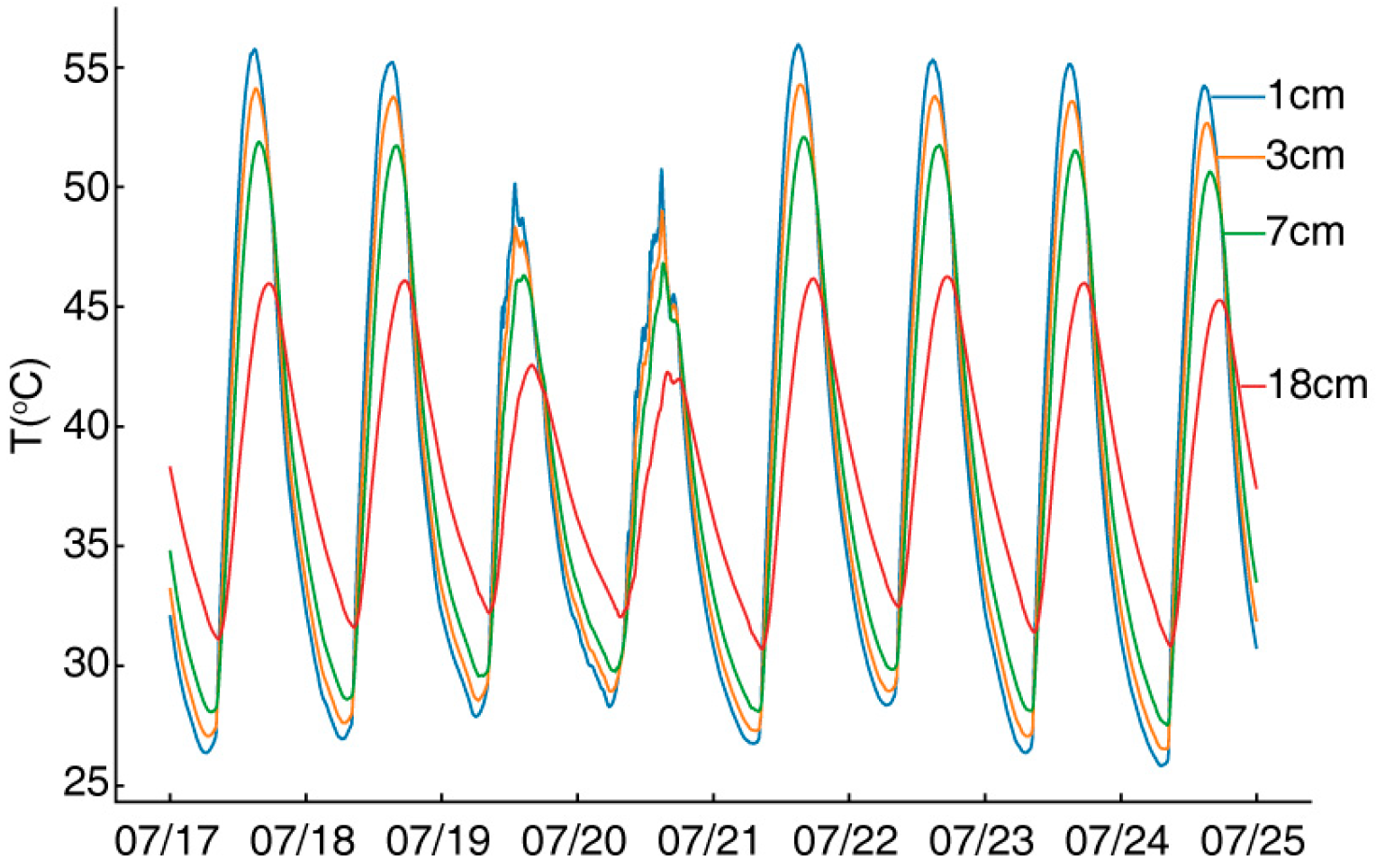
The pavement temperatures at depths of 1 cm, 3 cm, 7 cm, and 18 cm during the experiment are shown in Figure A1.
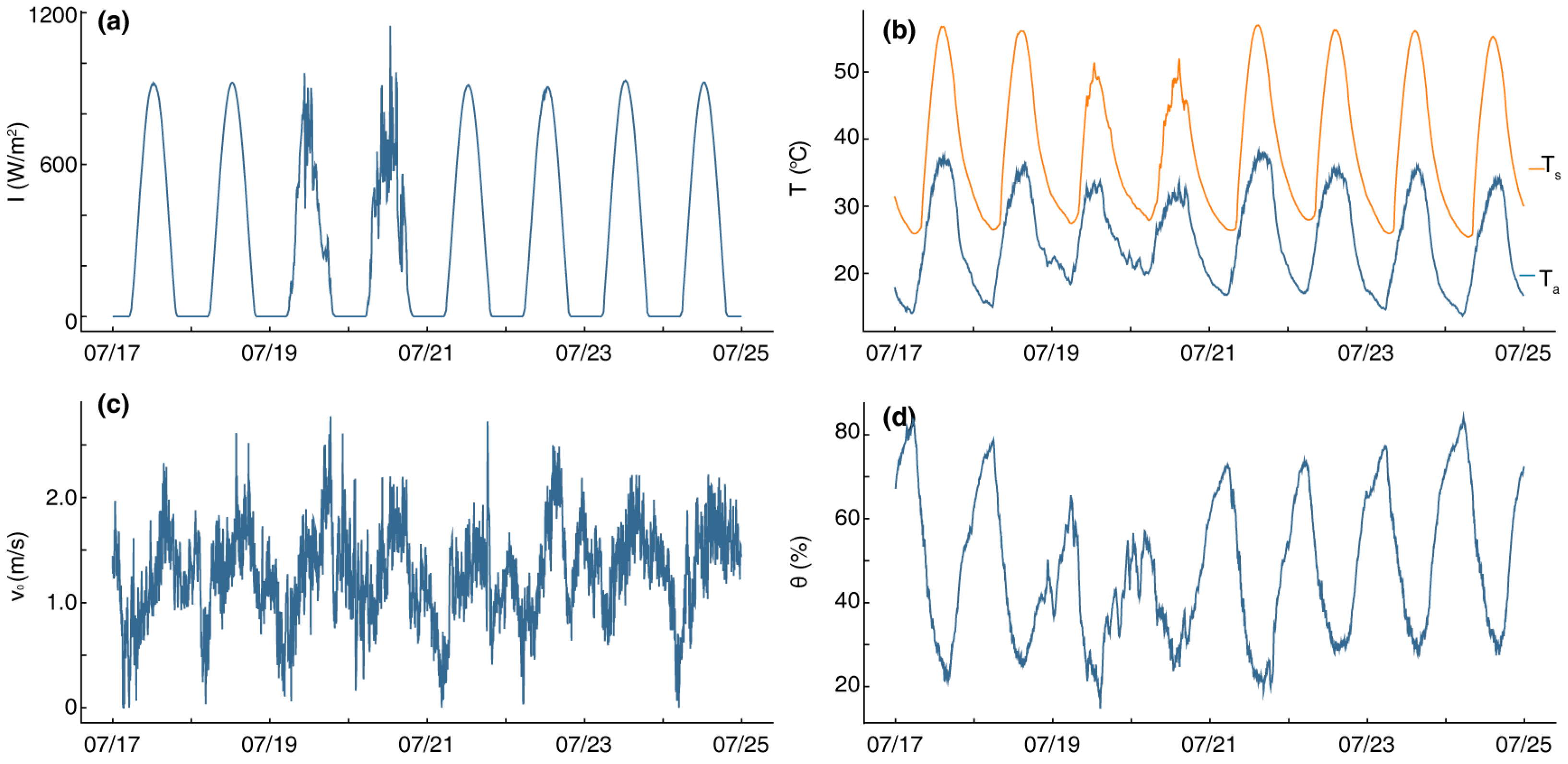
During the experiment, the incident solar radiation, air temperature, wind speed, and relative humidity were recorded in five minute interval and shown in Figure A2. In addition, the surface temperature estimated using the quadratic Maclaurin polynomial is also shown, accompanied by the air temperature.
Figure A1. Measured temperatures of pavement at depths of 1 cm, 3 cm, 7 cm, and 18 cm.
Infrastructures 11 00216 g0a1
Figure A2. Weather data. (a) I, (b) Ta and Ts, (c) vm, (d) θ.
Infrastructures 11 00216 g0a2

References

  1. Oke, T.; Cleugh, H. Urban heat storage derived as energy balance residuals. Bound.-Layer Meteorol. 1987, 39, 233–245. [Google Scholar] [CrossRef]
  2. Asaeda, T.; Ca, V.T.; Wake, A. Heat storage of pavement and its effect on the lower atmosphere. Atmos. Environ. 1996, 30, 413–427. [Google Scholar] [CrossRef]
  3. Yang, C.C.; Siao, J.H.; Yeh, W.C.; Wang, Y.M. A Study on Heat Storage and Dissipation Efficiency at Permeable Road Pavements. Materials 2021, 14, 3431. [Google Scholar] [CrossRef] [PubMed]
  4. Chen, J.; Wang, H.; Xie, P. Pavement temperature prediction: Theoretical models and critical affecting factors. Appl. Therm. Eng. 2019, 158, 113755. [Google Scholar] [CrossRef]
  5. Chen, J.; Zhang, M.; Wang, H.; Li, L. Evaluation of thermal conductivity of asphalt concrete with heterogeneous microstructure. Appl. Therm. Eng. 2015, 84, 368–374. [Google Scholar] [CrossRef]
  6. Gui, J.; Phelan, P.; Kaloush, K.; Golden, J. Impact of Pavement Thermophysical Properties on Surface Temperatures. J. Mater. Civ. Eng. 2007, 19, 683–690. [Google Scholar] [CrossRef]
  7. Qin, Y.; Hiller, J.E.; Meng, D. Linearity between Pavement Thermophysical Properties and Surface Temperatures. J. Mater. Civ. Eng. 2019, 31, 04019262. [Google Scholar] [CrossRef]
  8. Bentz, D.P. A Computer Model to Predict the Surface Temperature and Time-of-Wetness of Concrete Pavements and Bridge Decks; NISTIR 6551; National Institute of Standards and Technology: Gaithersburg, MD, USA, 2000. [Google Scholar]
  9. Uno, P.J. Plastic shrinkage cracking and evaporation formulas. ACI Mater. J. 1998, 95, 365–375. [Google Scholar] [CrossRef]
  10. Qin, Y.; Zhang, M.; Hiller, J.E. Theoretical and experimental studies on the daily accumulative heat gain from cool roofs. Energy 2017, 129, 138–147. [Google Scholar] [CrossRef]
  11. Bolton, D. The computation of equivalent potential temperature. Mon. Weather Rev. 1980, 108, 1046–1053. [Google Scholar] [CrossRef]
  12. Barber, E.S. Calculation of Maximum Pavement Temperatures from Weather Reports. Highw. Res. Bull. 1957, 168, 1–8. [Google Scholar]
  13. Qin, Y.; Hiller, J.E. Understanding pavement-surface energy balance and its implications on cool pavement development. Energy Build. 2014, 85, 389–399. [Google Scholar] [CrossRef]
  14. Qin, Y. Pavement surface maximum temperature increases linearly with solar absorption and reciprocal thermal inertial. Int. J. Heat Mass Transf. 2016, 97, 391–399. [Google Scholar] [CrossRef]
  15. Dan, H.-C.; Tan, J.-W.; Chen, J.-Q. Temperature distribution of asphalt bridge deck pavement with groundwater circulation temperature control system under high-and low-temperature conditions. Road Mater. Pavement Des. 2019, 20, 509–527. [Google Scholar]
  16. Wang, D.; Roesler, J.R.; Guo, D.-Z. Analytical approach to predicting temperature fields in multilayered pavement systems. J. Eng. Mech. 2009, 135, 334–344. [Google Scholar] [CrossRef]
  17. Adkins, D.F.; Merkley, G.P. Mathematical model of temperature changes in concrete pavements. J. Transp. Eng. 1990, 116, 349–358. [Google Scholar] [CrossRef]
  18. Jeong, J.-H.; Zollinger, D.G. Finite-element modeling and calibration of temperature prediction of hydrating Portland cement concrete pavements. J. Mater. Civ. Eng. 2006, 18, 317–324. [Google Scholar] [CrossRef]
  19. Li, H.; Harvey, J.; Jones, D. Development and preliminary validation of integrated local microclimate model for numerical evaluation of cool pavement strategies. Transp. Res. Rec. 2014, 2444, 151–162. [Google Scholar] [CrossRef]
  20. Solaimanian, M.; Kennedy, T.W. Predicting maximum pavement surface temperature using maximum air temperature and hourly solar radiation. Transp. Res. Rec. J. Transp. Res. Board 1993, 1417, 1–11. [Google Scholar]
  21. Hermansson, Å. Simulation Model for Calculating Pavement Temperatures Including Maximum Temperature. Transp. Res. Rec. J. Transp. Res. Board 2000, 1699, 134–141. [Google Scholar] [CrossRef]
  22. Dempsey, B.J. A Heat-Transfer Model for Evaluating Frost Action and Temperature Related Effects in Multilayered Pavement Systems; University of Illinois at Urbana-Champaign: Champaign, IL, USA, 1969. [Google Scholar]
  23. Mrawira, D.; Luca, J. Thermal Properties and Transient Temperature Response of Full-Depth Asphalt Pavements. Transp. Res. Rec. J. Transp. Res. Board 2002, 1809, 160–171. [Google Scholar] [CrossRef]
  24. Hermansson, Å. Mathematical model for paved surface summer and winter temperature: Comparison of calculated and measured temperatures. Cold Reg. Sci. Technol. 2004, 40, 1–17. [Google Scholar] [CrossRef]
  25. Teltayev, B.B.; Aitbayev, K. Modeling of transient temperature distribution in multilayer asphalt pavement. Geomech. Eng. 2015, 8, 133–152. [Google Scholar] [CrossRef]
  26. Minhoto, M.; Pais, J.; Pereira, P.; Picado-Santos, L. Predicting Asphalt Pavement Temperature with a Three-Dimensional Finite Element Method. Transp. Res. Rec. J. Transp. Res. Board 2005, 1919, 96–110. [Google Scholar] [CrossRef]
  27. Ho, C.-H.; Romero, P. Low design temperatures of asphalt pavements in dry–freeze regions: Predicting by means of solar radiation, transient heat transfer, and finite element method. Transp. Res. Rec. 2009, 2127, 60–71. [Google Scholar]
  28. Han, R.; Jin, X.; Glover, C.J. Modeling pavement temperature for use in binder oxidation models and pavement performance prediction. J. Mater. Civ. Eng. 2011, 23, 351–359. [Google Scholar] [CrossRef]
  29. Alavi, M.Z.; Pouranian, M.R.; Hajj, E.Y. Prediction of asphalt pavement temperature profile with finite control volume method. Transp. Res. Rec. 2014, 2456, 96–106. [Google Scholar] [CrossRef]
  30. Hall, M.; Dehdezi, P.; Dawson, A.; Grenfell, J.; Isola, R. Influence of the Thermophysical Properties of Pavement Materials on the Evolution of Temperature Depth Profiles in Different Climatic Regions. J. Mater. Civ. Eng. 2011, 24, 32–47. [Google Scholar]
  31. Hermansson, Å. Mathematical model for calculation of pavement temperatures: Comparison of calculated and measured temperatures. Transp. Res. Rec. 2001, 1764, 180–188. [Google Scholar] [CrossRef]
  32. Qin, Y.; Hiller, J.E. Modeling temperature distribution in rigid pavement slabs: Impact of air temperature. Constr. Build. Mater. 2011, 25, 3753–3761. [Google Scholar] [CrossRef]
  33. Qin, Y.; Hiller, J. Ways of formulating wind speed in heat convection significantly influencing pavement temperature prediction. Heat Mass Transf. 2013, 49, 745–752. [Google Scholar] [CrossRef]
  34. Nuijten, A.D. Runway temperature prediction, a case study for Oslo Airport, Norway. Cold Reg. Sci. Technol. 2016, 125, 72–84. [Google Scholar] [CrossRef]
  35. Denby, B.R.; Sundvor, I.; Johansson, C.; Pirjola, L.; Ketzel, M.; Norman, M.; Kupiainen, K.; Gustafsson, M.; Blomqvist, G.; Omstedt, G. A coupled road dust and surface moisture model to predict non-exhaust road traffic induced particle emissions (NORTRIP). Part 1: Road dust loading and suspension modelling. Atmos. Environ. 2013, 77, 283–300. [Google Scholar] [CrossRef]
Figure 1. Experimental design for the logging weather data and temperature of a pavement in Campus of Guangxi University. (a) Aerial view of the experiment site, (b) data-logging setup.
Infrastructures 11 00216 g001
Figure 2. Convergence of Maclaurin polynomial coefficients with increasing simulation iterations. (a) uncertainty of each coefficient, (b) the corresponding rates of uncertainty.
Infrastructures 11 00216 g002
Figure 3. Uncertainty of conductive heat flux (ΔG) and its contributing factors ( G x Δ x ). (a) A schematic diagram showing the heat flux at a pavement surface, (b) G x Δ x and ΔG, (c) mean and standard deviation of G x Δ x and ΔG, (d) box plot of G x Δ x and ΔG.
Infrastructures 11 00216 g003
Figure 4. Uncertainty of conductive heat flux (ΔG) and its contributing factors G k Δ k and G a 1 Δ a 1 . (a) A schematic diagram showing the calculation of heat flux at a pavement surface using measured temperature profile, (b) G k Δ k , G a 1 Δ a 1 , ΔG, (c) mean and standard deviation of G x Δ x and ΔG, (d) box plot of G x Δ x and ΔG.
Infrastructures 11 00216 g004
Table 1. Value and precision of the weather data and other information.
ItemTaθvIrek
Value----0.2250.901.57
Precision0.5 °C3%5% 5%0.020.010.1
Note: “-” means the values vary over time.
Table 2. Models available to estimate the heat convection coefficient.
Model Namehc ModelsNote
Vehrencamp model h c = 698.24 F ( 0.0014 T m ) 0.3 v d + 0.00097 ( T s T a ) 0.3
h c = 698.24 F ( 0.0014 T m ) 0.3 v d + 0.00097 | T s T a | 0.3
F = 1.0, d = 0.7 [20,21,22,23,24,25,26,27]
F = 1.4, d = 0.5 [28,29,30]
F = 1.1, d = 0.5 [31]
Empirical model h c = 5.678 ( 1.3 + 1.135 v 0.75 ) [12]
h c = { 5.6 + 4.0 v v     5 7.2 v 0.78 v   >   5 [8,13,14,15]
h c = 6 + 3.7 v   or   6.1 + 3.7 v 0.2 [16,17,18,19]
Flat plate model h c = 0.664 k a P r a 0.3 v a 0.5 L c 0.5 v 0.5 [6]
h c = 5.6 + 0.332 P r a 0.3 v a 0.5 L c 0.5 v 0.5 [32,33]
Denby model h c = ρ a C p / r a [34,35]
Note: Tm = 0.5(TsTa) + 273.15, v0.2 = wind speed measured at 0.2 m height; Cp = heat capacity of dry air; ka = air thermal conductivity, υa is air kinematic viscosity; Lc = characteristic length of the flat plate; ra = aerodynamic resistance for temperature (s·m−1). Subscript a = air.
Disclaimer/Publisher’s Note: The statements, opinions and data contained in all publications are solely those of the individual author(s) and contributor(s) and not of MDPI and/or the editor(s). MDPI and/or the editor(s) disclaim responsibility for any injury to people or property resulting from any ideas, methods, instructions or products referred to in the content.