Dynamic Simulation of Seismogenic-Fault-Induced Rupture in Overlying Soil

Abstract

Accurate prediction of surface rupture induced by seismogenic fault displacement is essential for the seismic safety assessment of major engineering projects. Most existing numerical simulations adopt quasi-static approaches, in which the effect of fault displacement is simplified as static loading. As a result, these methods cannot represent the dynamic characteristics of the fault rupture process, such as stress-wave propagation, soil inertial effects, and the influence of dynamic loading paths on rupture extension in soil layers. To address this issue, a full-process simulation method is established for simulating rupture of overlying soil subjected to dynamic fault displacement: Firstly, a non-uniform dynamic fault displacement loading is formulated for the two sides of the fault based on viscoelastic artificial boundaries, allowing the differential motion of the bedrock on both sides of the fault to be represented. Secondly, an improved dynamic skeleton curve constitutive model of soil is developed by introducing a minimum modulus constraint, providing an improved description of soil nonlinear dynamic behavior from small-strain hysteresis to large-strain shear failure. The reliability of the proposed method is verified through element-level tests and horizontal-site response simulation. As a benchmark, its ability to reproduce key rupture characteristics under quasi-static conditions is also assessed by comparison with classical quasi-static rupture studies. The method is then applied to simulate rupture extension and deformation response of overlying soil under strike-slip fault displacement. The results show that, compared to quasi-static analysis, dynamic fault displacement produces similar cumulative slip for surface rupture initiation and full connection, but induces transient amplification of peak surface displacement and a wider deformation zone with gentler displacement gradients. These findings demonstrate the necessity of considering dynamic fault dislocation of bedrock–overlying soil interaction in seismic assessments of engineering projects crossing active faults.

1. Introduction

During earthquakes, fault dislocation originating from seismogenic processes often induces dynamic rupture and severe deformation within the overlying soil layers, which in turn poses serious threats to engineering structures situated on or near active faults. Therefore, establishing a dynamic analysis framework to elucidate how rupture initiates and extends within the overlying soil is essential for improving seismic design and performing reliable risk assessments of fault-crossing projects. In particular, deformation patterns at the ground surface and near-surface layers largely determine the extent of structural damage, underscoring the need to examine soil mechanical behavior under dynamic fault-induced loading.

Previous research regarding fault dislocation in overlying soils has generally involved three main methodological directions: statistical analysis, experimental simulation, and numerical simulation. The statistical analysis method establishes empirical correlations between earthquake magnitude and rupture parameters such as surface displacement and rupture length, using historical seismic data (e.g., Tocher, Bonilla, and Coppersmith [1,2,3]). Although these correlations enable efficient regional assessment, the dependability of their results relies heavily on record accuracy and data completeness, and they usually fail to incorporate differences in soil characteristics or fault mechanisms. The experimental simulation, including centrifuge tests (Bransby, Ng, Shen, Guo et al. [4,5,6,7]) and sandbox model tests (Sanford, Johansson, Shi et al. [8,9,10,11]), can visually reproduce soil rupture processes and clarify the influence of factors such as soil thickness and density, but is constrained by test equipment limitations, cost, and model scale.

Owing to its manageable cost, stable repeatability, and flexibility for complex geological settings, numerical simulation has become the principal analytical method for this topic. By applying the finite-element technique, Bray, Loukidis, Oettle, Loli, Lin, and Li [12,13,14,15,16,17,18] explored the rupture extension within homogeneous overlying soils, focusing on the influence of fault type, dip angle, and soil properties on rupture trace and surface deformation. Zanjani, Oettle, and Zhao [19,20,21,22,23] extended the discussion to layered ground conditions, while Garcia et al. [24] investigated soil heterogeneity through discrete-element models, and Jella et al. [25] performed parametric finite-element analyses incorporating recorded ground motions.

Beyond free-field conditions, the presence of structures has been shown to significantly influence fault rupture propagation. Centrifuge tests and numerical analyses by Bransby et al. [4], Loli et al. [17], Oettle et al. [20], and Agalianos et al. [26] have demonstrated that structures can alter rupture paths and surface deformation patterns through complex soil–structure interaction. In engineering practice, the quantitative assessment of fault rupture hazard is typically addressed via probabilistic frameworks, as exemplified by standards such as AESJ-SC-RK009:2021 [27] and ANSI/ANS-2.30-2015 [28], which incorporate conservative assumptions to envelope epistemic uncertainties and provide a practical basis for critical facility siting and design. Collectively, these studies have greatly improved the comprehension of fault-induced rupture in soil layers.

Nevertheless, most numerical simulation studies still rely on static or quasi-static assumptions, where fault dislocation at the bedrock level is modeled as a gradually applied boundary load, thereby overlooking the dynamic essence of seismic rupture. In real earthquakes, fault movement is a transient process involving stress-wave propagation, inertial effects, and highly nonlinear soil behavior under rapid loading conditions. Neglecting these mechanisms may lead to inaccurate representation of rupture evolution, instantaneous strain peaks, and dynamic wave interactions, thereby introducing potential uncertainties into the simulation outcomes.

More recently, Wang et al. [29] developed a 2D dynamic simulation framework for dip-slip faults (normal and reverse), demonstrating the necessity of considering dynamic effects through comparisons with quasi-static analyses. However, their work adopts a nonlinear elastic constitutive model, which leads to two inherent limitations: (1) soil strain recovers immediately as the bedrock displacement decreases after reaching its peak, failing to capture permanent deformation, and (2) the absence of an energy dissipation mechanism results in prolonged oscillations in the large-strain zone caused by wave superposition from non-uniform inputs on the two sides of the fault. Moreover, their study focuses exclusively on dip-slip faults, where fault movement is perpendicular to the strike and the site response can be reasonably analyzed using 2D plane-strain models.

To overcome these limitations and extend the analysis to more complex faulting mechanisms, this study establishes a unified numerical analysis framework for simulating the full dynamic process of fault-induced rupture in overlying soil. The main methodological contributions are as follows: (1) an improved dynamic skeleton curve constitutive model is developed by introducing a minimum modulus constraint to better describe nonlinear soil behavior from small-strain hysteresis to large-strain shear failure, addressing the limitations of nonlinear elastic models in capturing permanent deformation and energy dissipation; (2) a 3D non-uniform dynamic fault loading method based on viscoelastic artificial boundaries is proposed to represent the dynamic action associated with fault displacement on both sides of the fault, enabling realistic simulation of strike-slip fault dislocation. The framework is validated against quasi-static results, and the comparisons demonstrate that dynamic effects can markedly alter rupture extension patterns, surface displacement fields, and deformation localization. These findings highlight the necessity of adopting a 3D dynamic analysis framework for accurate seismic risk assessment of engineering projects crossing active faults, particularly in strike-slip settings.

2. Methods

To accurately simulate the nonlinear response and rupture evolution of overlying soils under dynamic fault slip, this section presents two complementary methodological components. The first is a modified dynamic skeleton curve constitutive model, and its constitutive integration is implemented in ABAQUS/Explicit (version 2021) via a VUMAT subroutine. The second is a three-dimensional non-uniform-input scheme for prescribing differential bedrock motions on opposite sides of the fault. Taken together, these developments form a fully coupled dynamic simulation framework for investigating the complete rupture process of the overlying soil under different faulting mechanisms, including dip-slip and strike-slip events.

2.1. Modified Dynamic Skeleton Curve Constitutive Model of Soil

The constitutive model adopted in this study is derived from the dynamic skeleton curve constitutive model proposed by Li [30,31] and is further modified to be applicable to large-deformation conditions. Compared with traditional Masing-type models, the dynamic skeleton curve constitutive model significantly simplifies the logical judgment and computational implementation of complex loading–unloading paths, while retaining their physical rationality. While reasonably capturing the dynamic characteristics of soils, the model exhibits good numerical extensibility and stability, enabling it to be coupled with the aforementioned non-uniform-input method to achieve fully coupled dynamic simulations of fault rupture–soil response.

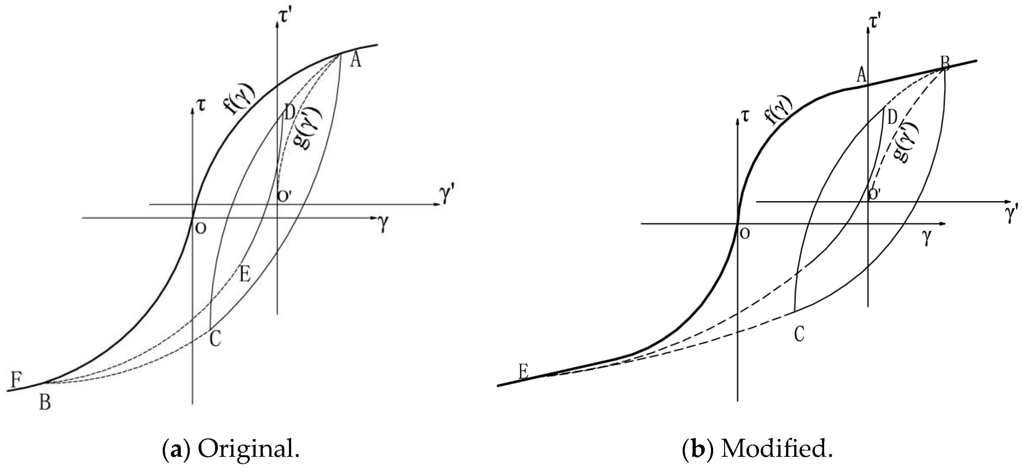
The defining characteristic of the dynamic skeleton curve is that the skeleton curve evolves with the stress–strain history. The fundamental idea can be summarized as follows. During the initial loading stage, as well as during subsequent loading stages in which the absolute strain exceeds the previously attained maximum absolute strain, the response follows the initial skeleton curve. For unloading or reverse loading from any loading state, the path is directed toward the historical maximum turning point (τ_M, γ_M), or its symmetric counterpart (−τ_M, −γ_M), and the resulting curve maintains a form similar to that of the skeleton curve, as shown in Figure 1a.

The original dynamic skeleton curve model proposed by Li and Liao [27] is expressed in Equation (1), which defines two types of curves: the dynamic skeleton curve for |γ| ≤ γ_M (representing unloading/reloading paths directed toward the historical maximum point) and the initial skeleton curve for |γ| > γ_M (representing first-time loading or loading beyond the historical maximum strain).

$$\tau (\gamma )\left\{\begin{array}{c}={\tau }_{\mathrm{c}}+{\displaystyle \frac{G_0\left(\gamma -{\gamma }_{\mathrm{c}}\right)}{1+\left|\left(\gamma -{\gamma }_{\mathrm{c}}\right)/2{\gamma }_{\mathrm{r}}^{\prime }\right|}} , \left|\gamma \right|\le {\gamma }_{\mathrm{M}}\\ ={\displaystyle \frac{G_0\gamma }{1+\left|\gamma \right|/{\gamma }_{\mathrm{r}}}} , \left|\gamma \right|>{\gamma }_{\mathrm{M}}\end{array}\right.$$

(1)

where γ_r is the reference shear strain and G₀ denotes the maximum dynamic shear modulus of the soil. The parameter ${\gamma }_{\mathrm{r}}^{\prime }$ is a curve control parameter, which can be expressed as

$${\gamma }_{\mathrm{r}}^{\prime }={\left[{\displaystyle \frac{\pm 2G_0}{\pm {\tau }_{\mathrm{M}}-{\tau }_{\mathrm{c}}}}-{\displaystyle \frac{\pm 2}{\pm {\gamma }_{\mathrm{M}}-{\gamma }_{\mathrm{c}}}}\right]}^{-1}$$

(2)

In Equation (2), the sign “±” indicates that the “+” sign is adopted when the increment of shear strain Δγ is positive, and the “−” sign is adopted otherwise. (τ_M, γ_M) represents the historical maximum point in terms of absolute values, while (τ_c, γ_c) denotes the last turning point prior to the current.

For the original skeleton curve (Equation (1)), the shear modulus approaches zero as the strain tends to infinity, which may cause numerical instability and element distortion in ABAQUS/Explicit analyses. To address this issue, a minimum modulus constraint is introduced, with the minimum modulus taken as 1% of the initial modulus, ensuring numerical stability while approximately capturing the residual strength behavior of soil. It is emphasized that this coefficient is a numerical stabilization measure rather than a material property; the smaller the coefficient, the closer the response approximates ideal material softening. The specific value of 1% was determined through trial calculations: for the materials used in the comparative cases of this study, the coefficient was gradually reduced from 10% to 1%. When the coefficient fell below 1%, the model exhibited element distortion and the analysis terminated. Therefore, all comparative cases in this study uniformly adopt 1% to ensure result comparability.

Accordingly, the modified initial skeleton curve is defined in a piecewise form: once the shear strain exceeds a threshold value γ_y and the modulus degrades to the minimum value, the constitutive response transitions to a linear-elastic stage with a slope equal to the minimum modulus. Since the modulus of the dynamic skeleton curve is theoretically higher than that of the initial skeleton curve, no modification is applied to the dynamic skeleton curve. The modified constitutive model is illustrated in Figure 1b.

Specifically, the modified initial skeleton curve is given in Equation (3) as a piecewise function that incorporates the minimum modulus constraint, while the dynamic skeleton curve remains unchanged as given in Equation (4).

$$\tau (\gamma )\left\{\begin{array}{c}={\displaystyle \frac{G_0\gamma }{1+\left|\gamma \right|/{\gamma }_{\mathrm{r}}}} , \gamma \le {\gamma }_{\mathrm{y}}\\ ={\tau }_{\mathrm{y}}+0.01\times G_0\times \left(\gamma -{\gamma }_{\mathrm{y}}\right) , \gamma >{\gamma }_{\mathrm{y}}\end{array}\right.$$

(3)

$$\tau (\gamma )={\tau }_{\mathrm{c}}+{\displaystyle \frac{G_0\left(\gamma -{\gamma }_{\mathrm{c}}\right)}{1+\left|\left(\gamma -{\gamma }_{\mathrm{c}}\right)/2{\gamma }_{\mathrm{r}}^{\prime }\right|}}$$

(4)

In Equations (3) and (4), the constitutive response is expressed in terms of the equivalent shear stress and equivalent shear strain. Based on these relationships, the shear modulus at each increment can be evaluated and used to update the Jacobian matrix, thereby determining the stress tensor at each incremental step:

$$\Delta \left[\begin{array}{c}{\sigma }_{11}\\ {\sigma }_{22}\\ {\sigma }_{33}\\ {\sigma }_{12}\\ {\sigma }_{23}\\ {\sigma }_{13}\end{array}\right]=\left[\begin{array}{cccccc}\lambda +2\mu & \lambda & \lambda & 0& 0& 0\\ \lambda & \lambda +2\mu & \lambda & 0& 0& 0\\ \lambda & \lambda & \lambda +2\mu & 0& 0& 0\\ 0& 0& 0& \mu & 0& 0\\ 0& 0& 0& 0& \mu & 0\\ 0& 0& 0& 0& 0& \mu \end{array}\right]·\Delta \left[\begin{array}{c}{\epsilon }_{11}\\ {\epsilon }_{22}\\ {\epsilon }_{33}\\ {2\epsilon }_{12}\\ {2\epsilon }_{23}\\ {2\epsilon }_{13}\end{array}\right]$$

(5)

where λ and μ are the Lamé constants:

$$\lambda ={\displaystyle \frac{2G^{t+\mathit{\Delta }t}\nu }{1-2\nu }}\hspace{1em}\hspace{1em}\mu =G^{t+\mathit{\Delta }t}$$

(6)

Here, ν is Poisson’s ratio, and G^t+Δt is the tangent shear modulus at the current increment.

The equivalent shear strain is calculated as

$${\gamma }_{\mathrm{e}\mathrm{q}}^{t+\mathit{\Delta }t}={\gamma }_{\mathrm{e}\mathrm{q}}^t+s\times \left|\Delta {\gamma }_{\mathrm{e}\mathrm{q}}^{t+\mathit{\Delta }t}\left({\epsilon }^0\right)\right|,{\epsilon }^0=\epsilon -{\epsilon }_{\mathrm{c}}$$

(7)

$$\Delta {\gamma }_{\mathrm{e}\mathrm{q}}^{t+\mathit{\Delta }t}\left({\epsilon }^0\right)={\gamma }_{\mathrm{o}\mathrm{c}\mathrm{t}}^{t+\mathit{\Delta }t}\left({\epsilon }^0\right)-{\gamma }_{\mathrm{o}\mathrm{c}\mathrm{t}}^t\left({\epsilon }^0\right)$$

(8)

where γ_oct denotes the octahedral shear strain; ${\gamma }_{\mathrm{e}\mathrm{q}}^{t+\mathit{\Delta }t}$ and ${\gamma }_{\mathrm{e}\mathrm{q}}^t$ are the equivalent shear strains at the current and previous time steps, respectively; $\Delta {\gamma }_{\mathrm{e}\mathrm{q}}^{t+\mathit{\Delta }t}$ is the increment of equivalent shear strain at the current time step; ε⁰ represents the strain tensor corresponding to the current strain ε relative to the most recent turning point strain ε_c; and s takes a value of 1 during loading and −1 during unloading. The turning point of the skeleton curve is identified based on the sign of the increment of equivalent shear strain. A curve reversal is detected within an incremental step when the increment of equivalent shear strain becomes negative.

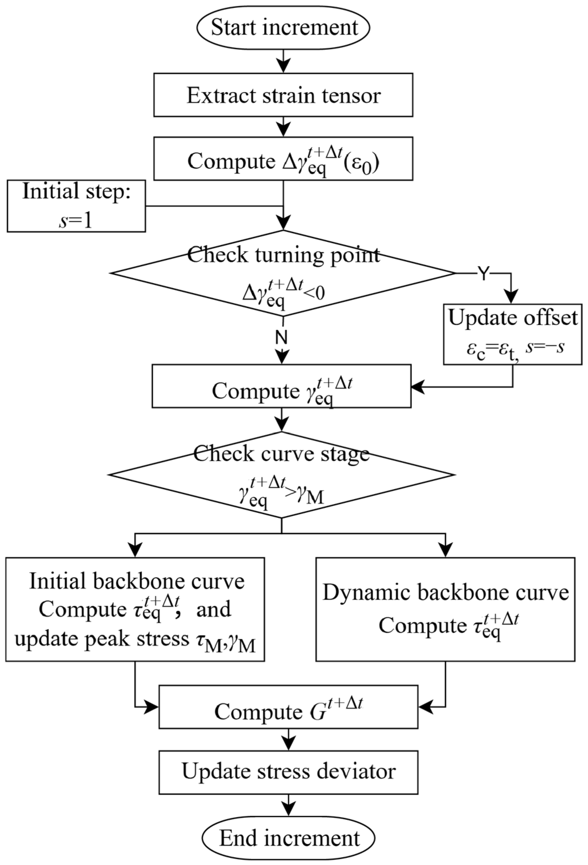
The modified dynamic skeleton curve constitutive model of soil was implemented in the ABAQUS/Explicit solver through user subroutine development. The computational procedure of the VUMAT subroutine is illustrated in Figure 2.

2.2. Non-Uniform Dynamic Input Method Across Faulted Sites

The core idea of the three-dimensional non-uniform dynamic input is as follows. The seismic-wave incidence is constrained to be parallel to the fault dip plane; the fault surface is modeled as a smooth contact interface; and the back-interaction of scattered, outward-propagating waves from the finite domain on the free-field response of the opposite semi-infinite domain is neglected. Under these assumptions, the far-field input motions on the two sides of the fault can be determined independently from their respective free-field responses. In the numerical implementation, the corresponding free-field ground motions are imposed on the bottom boundary and on the left/right side boundaries associated with each fault block, so that differential motions across the fault and their mutual interaction develop naturally within the finite domain.

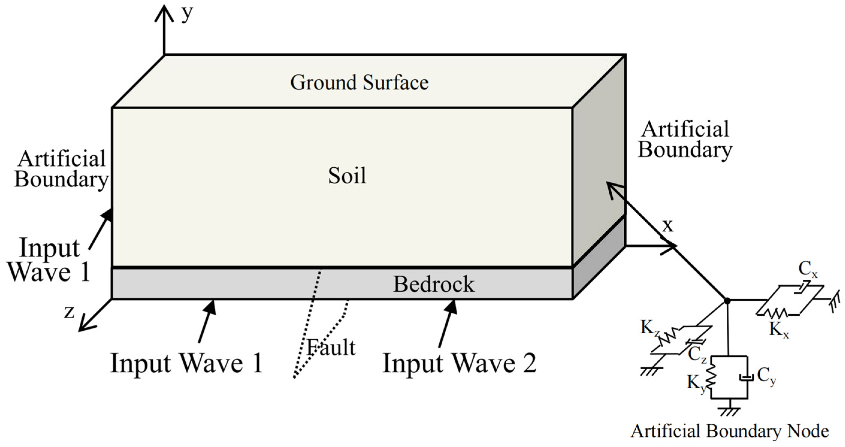
The boundary configuration of the three-dimensional model and the input locations are shown in Figure 3. Except for the free ground surface, viscoelastic artificial boundaries are used on the bottom surface and the four lateral surfaces. The fault plane divides the bottom boundary into two parts, and the left/right side boundaries correspond to the two fault sides; thus, free-field motions on each side are applied to the bottom and the corresponding side boundary to produce non-uniform excitation across the fault. In contrast, since no preset rupture is introduced in the overlying layers, it is difficult to partition the front/back boundaries along the fault trace. To avoid extra partitioning and free-field matching, only oblique incidence in planes perpendicular to the z-axis, or vertical incidence from the bottom boundary, is considered. Accordingly, incident motions are applied only on the bottom and left/right side boundaries, while the front/back boundaries act only as radiation boundaries. Under this constraint, boundary points with the same (x, y) but different z coordinates receive the same input, which simplifies the implementation of three-dimensional non-uniform input.

For the boundary nodes on the bottom and left/right side surfaces, the nodal dynamic equilibrium including the viscoelastic boundary forces is given by Equation (9).

$$M\ddot{u}+(C+A_{\mathrm{B}}{C}_{\mathrm{B}})\dot{u}+(K+A_{\mathrm{B}}{K}_{\mathrm{B}})u=f_1+f_2$$

(9)

where K_B and C_B are the spring stiffness and damping coefficients of the viscoelastic boundary; M, C, and K represent the mass, damping, and stiffness matrices, respectively; in the present free-field boundary analysis, C is set to zero (i.e., internal damping within the domain is neglected), and far-field energy dissipation is represented only by the boundary-damping coefficient C_B; u, $\dot{u}$ and $\ddot{u}$ denote the node displacement, velocity, and acceleration, respectively; and f is the applied node force. The parameter A_B is the control area for the viscoelastic boundary node.

The total force f acting on a boundary node is decomposed into two components:

• f₁, the force required for the artificial boundary node to achieve a displacement u^I against the resistance of the finite domain medium, determinable via the geometric and constitutive relations of the internal medium;
• f₂, the force required to achieve the same displacement u^I against the boundary spring–dashpot elements. This force is derived from the incident displacement field uI at the artificial boundary within the viscoelastic framework:

$$f_2=A_{\mathrm{B}}\left(K_{\mathrm{B}}{u}^{\mathrm{I}}+C_{\mathrm{B}}{\dot{u}}^{\mathrm{I}}\right)$$

(10)

To define the viscoelastic boundary terms in Equations (9) and (10), viscoelastic artificial boundaries [32,33,34] are adopted by attaching spring–dashpot components to each boundary node in all directions. The dashpots absorb the energy of outgoing waves, while the springs provide the corresponding restoring forces, thereby simulating the mechanical response of an infinite surrounding medium. The boundary spring stiffness K_B and damping coefficient C_B are computed using Equation (11) for 2D models and Equation (12) for 3D models. The control area A_B is defined as half of the connected boundary edge length in 2D and one-quarter of the connected boundary face area in 3D.

$$Normal:\hspace{1em}\hspace{1em}{K}_{\mathrm{B}}={\displaystyle \frac{1}{1+A}}·{\displaystyle \frac{\lambda +2\mu }{2r}},C_{\mathrm{B}}=B\rho c_{\mathrm{p}}$$

(11a)

$$Tangential: \hspace{1em}\hspace{1em}{K}_{\mathrm{B}}={\displaystyle \frac{1}{1+A}}·{\displaystyle \frac{\mu }{2r}},C_{\mathrm{B}}=B\rho c_{\mathrm{s}}$$

(11b)

$$Normal:\hspace{1em}\hspace{1em}{K}_{\mathrm{B}}={\displaystyle \frac{1}{1+A}}·{\displaystyle \frac{\lambda +2\mu }{r}},C_{\mathrm{B}}=B\rho c_{\mathrm{p}}$$

(12a)

$$Tangential: \hspace{1em}\hspace{1em}{K}_{\mathrm{B}}={\displaystyle \frac{1}{1+A}}·{\displaystyle \frac{\mu }{r}},C_{\mathrm{B}}=B\rho c_{\mathrm{s}}$$

(12b)

where λ and μ are the Lamé constants, ρ is the mass density, and c_p and c_s are the P-wave and S-wave velocities, respectively. The distance r is taken from the geometric center of the near-field structure to the boundary segment, and in this study r is taken as half of the model thickness. The artificial boundary parameters A and B were adopted from the viscoelastic boundary model proposed by Du et al. [32], in which A = 0.8 and B = 1.1 were recommended based on theoretical derivation and numerical verification.

In summary, the three-dimensional non-uniform input is implemented by applying fault-side free-field equivalent nodal forces, together with the matching viscoelastic spring–dashpot parameters, on the bottom and left/right side boundaries, while treating the front/back boundaries as purely absorbing boundaries without incident input. This setup provides a practical and directly implementable boundary-input procedure for subsequent dynamic response analyses of three-dimensional strike-slip faulted sites.

3. Validation of the Proposed Framework

This section presents a hierarchical validation of the proposed nonlinear dynamic-rupture simulation framework and its numerical implementation (modified dynamic backbone-curve constitutive model and 3D viscoelastic artificial boundaries with an across-fault non-uniform-input scheme). The verification proceeds from material constitutive behavior to boundary input, site response, and fault rupture patterns, as follows:

(1) Element-scale shear tests: Stress–strain relations from pure-shear loading–unloading cycles are used to examine whether the constitutive model reproduces hysteretic energy dissipation at small strains and stiffness degradation with residual strength at large strains, and to assess the stability and correctness of the VUMAT implementation.

(2) Verification of the 3D boundaries and non-uniform input: A 3D homogeneous linear-elastic model is excited by a vertically incident Gaussian pulse applied at the base. Both uniform input and spatially partitioned, time-delayed non-uniform input are simulated. The expected twofold free-surface amplification and the displacement time histories at different locations on the top surface are compared to validate the 3D viscoelastic boundary setup and the non-uniform-input procedure.

(3) Verification of seismic response of a horizontally layered site: Strong-motion recordings from the Xiangtang array are used as the incident bedrock motion (within/borehole record) applied at the model base. Surface acceleration time histories and response spectra are obtained and compared with the recorded surface motions and equivalent-linear results, to evaluate the capability of the proposed method to capture site response and nonlinear energy dissipation under irregular earthquake excitation.

(4) Quasi-static comparison studies: A suite of quasi-static reverse-fault cases is first analyzed to reproduce rupture propagation in the overlying soil for different fault dips and fault types, followed by qualitative and quantitative comparisons with published benchmark results. An existing strike-slip fault physical-model test configuration is then reproduced numerically. The planform geometry and width of the surface rupture (deformation) zone and the along-strike slip distribution are compared to assess the ability of the proposed 3D strike-slip fault framework to capture rupture-zone geometry and slip characteristics.

These multi-level validations provide a consistent and traceable numerical basis for subsequent simulations of dip-slip and three-dimensional strike-slip fault dynamic rupture processes, as well as comparative analyses against quasi-static results.

3.1. Constitutive Model Verification: Element-Level Cyclic Shear Test

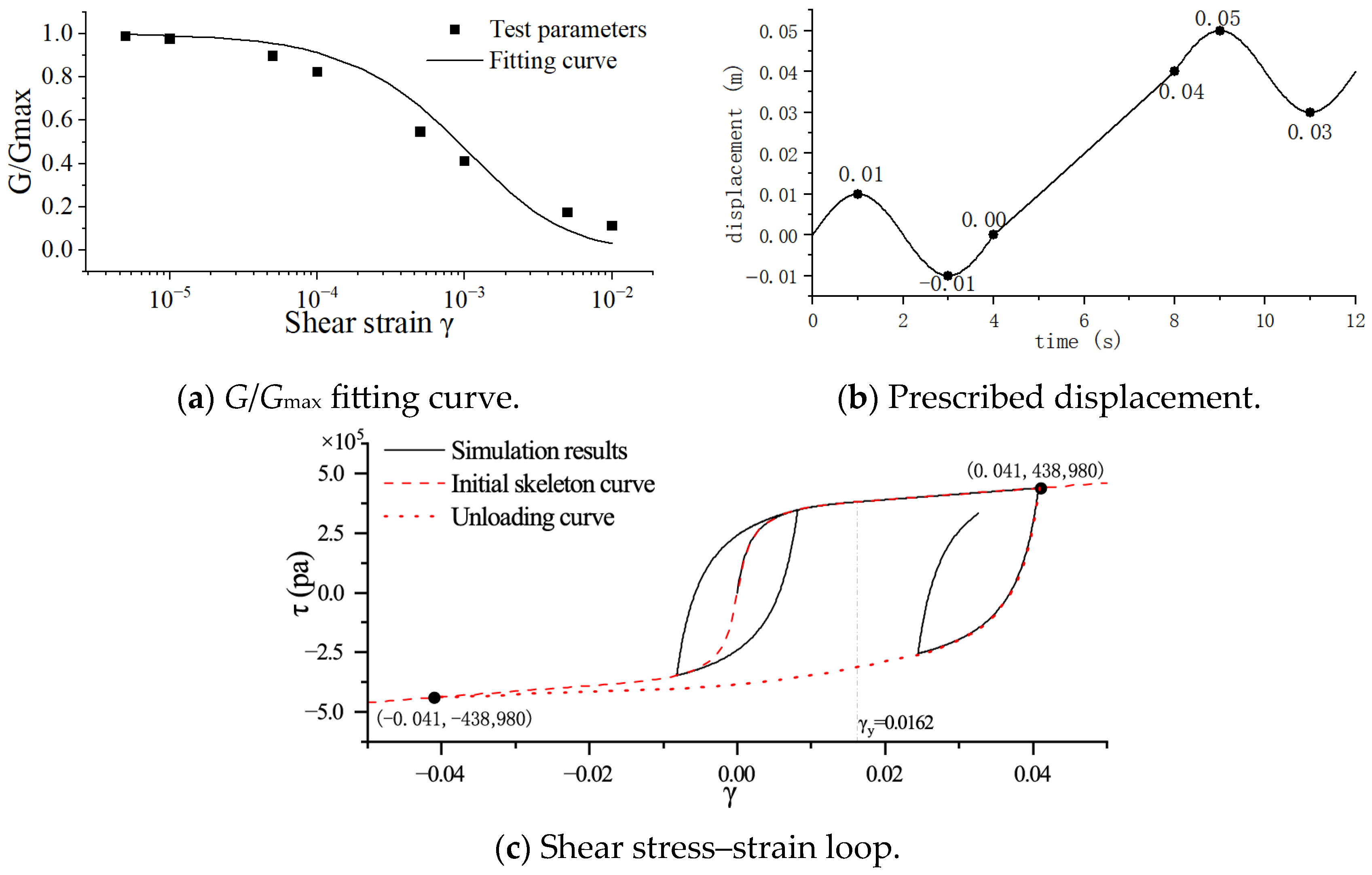
To verify the correctness of the proposed constitutive model and its implementation in the VUMAT subroutine, a single-element shear simulation was conducted. A plane-strain element with dimensions of 1 m × 1 m was employed. The bottom of the element was fully fixed, while a horizontal displacement was applied at the top to induce a state of pure shear. The physical and mechanical properties of the element are summarized in

Table 1. Physical and mechanical properties of the single element.

Material	ρ (kg/m3)	vs (m/s)	Gmax (Pa)	ν	c (kPa)	φ (°)	γr
Sand	2000	340	2.35 × 108	0.3	0.0	33.0	0.0018

. The reference shear strain γ_r was determined by fitting the G/G_max-γ relationship listed in

Table 2. Shear modulus degradation parameters.

Shear Strain γ	5 × 10−6	1 × 10−5	5 × 10−5	1 × 10−4	5 × 10−4	1 × 10−3	5 × 10−3	1 × 10−2
G/Gmax	0.9880	0.9760	0.8980	0.8230	0.5470	0.4120	0.1740	0.1130
λ	0.0110	0.0121	0.0198	0.0270	0.0537	0.0669	0.0907	0.0969

. Specifically, the tangent modulus derived from Equation (3) is expressed as a function of γ, and γ_r is determined through least-squares fitting to the G/G_max values in Table 2, with the fitted curve shown in Figure 4a. It should be noted that the damping ratios λ in Table 2 are not input parameters but are provided as reference data indicating typical damping characteristics of soils.

The prescribed displacement history is shown in Figure 4b and consists of three stages. The first and third stages correspond to sinusoidal loading with an amplitude of 0.01 m, while the second stage applies monotonic loading until the shear displacement at the top of the element reaches 0.04 m.

The simulated shear stress–strain response of the element is shown in Figure 4c. Pronounced hysteretic damping behavior is observed at small-strain levels, whereas at large strains the response exhibits a linear-elastic behavior with preserved residual strength. The stress–strain curve during the initial and monotonic loading stages closely follows the theoretical initial skeleton curve, and the unloading curve after monotonic loading conforms to the theoretical dynamic skeleton curve directed toward the historical maximum point. Overall, the results confirm that the developed VUMAT subroutine successfully reproduces the intended nonlinear hysteresis at small strains and the elastic response at large strains.

3.2. Verification of the Three-Dimensional Non-Uniform-Input Method

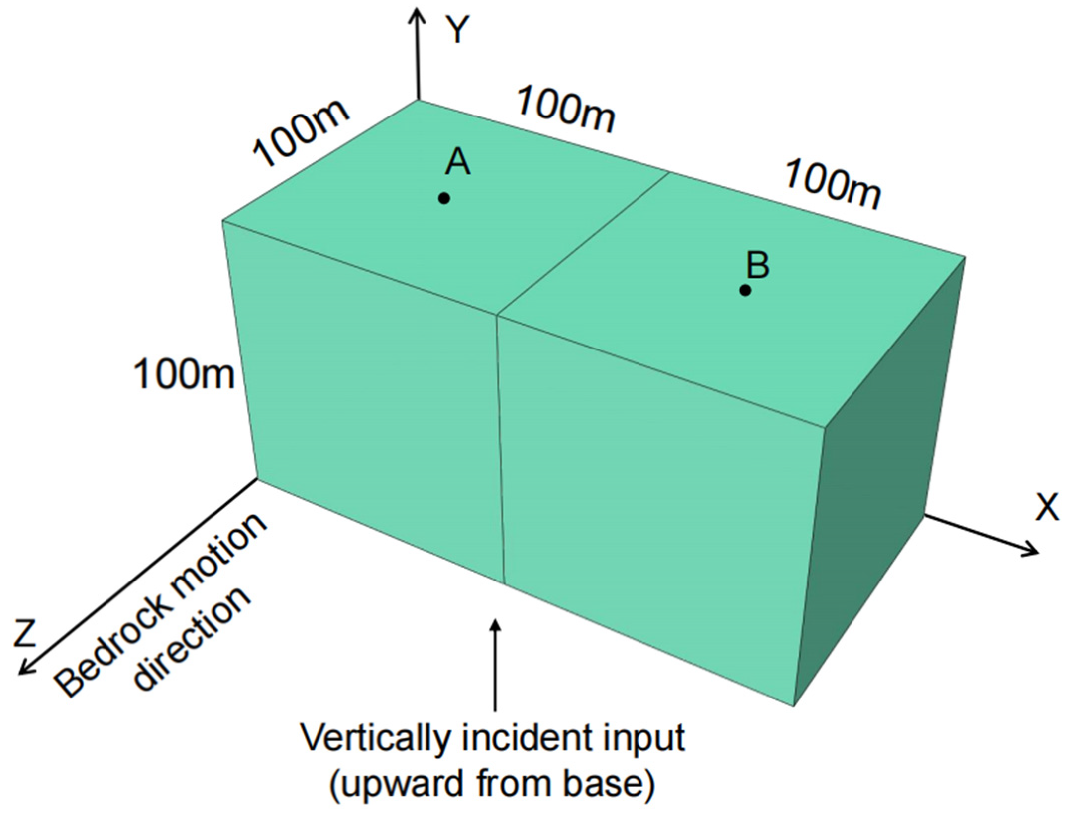
To verify the 3D viscoelastic artificial boundary configuration and the implementation of the non-uniform input procedure, a 3D homogeneous linear-elastic model is established for comparative simulations (Figure 5). The model dimensions are 200 m × 100 m × 100 m. A vertically incident motion is applied at the model base, using a Gaussian pulse with an effective duration of 1 s. The material is assumed to be linear elastic, and the parameters are listed in

Table 3. Material parameters for the verification model.

Soil Type	ρ (kg/m3)	vs (m/s)	Gmax (Pa)	ν
Sand	2000	340	2.35 × 108	0.3

.

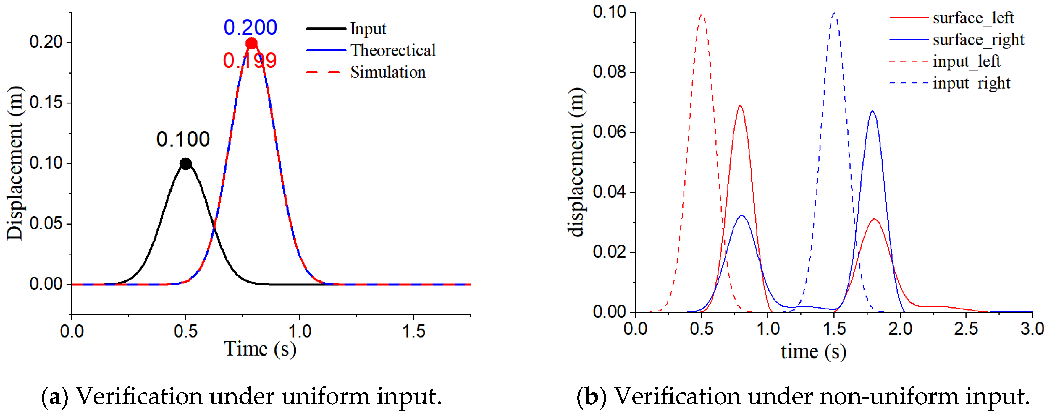
(1) Verification under uniform input

Under the uniform-input condition, identical pulse motions are applied over the entire base. The displacement time history at the center of the top surface is extracted, as shown in Figure 6a. The simulated displacement at the top-center point closely follows the theoretical free-surface response (amplification factor of 2 at the free surface of a homogeneous elastic half-space). This indicates that the boundary setup and wave-input implementation are correct for uniform input.

(2) Verification under non-uniform input (partitioned time-delayed input)

The non-uniform-input implementation is further examined. As illustrated in Figure 5, the model is split into left and right halves by the mid-plane perpendicular to the x axis (x = Lx/2). The same Gaussian pulse is applied to both halves, while the input on the right half is delayed by 1 s. Displacement time histories at points A and B (located at the centers of the left and right halves of the top surface, respectively) are extracted (Figure 6b). During 0–1 s, only the left-half input is active: the response at point A appears first and its amplitude is lower than the incident amplitude, while point B records low-amplitude waves propagating from left to right. After 1 s, when the right-half input starts, the displacement amplitude at point B increases markedly, and point A correspondingly records waves propagating from right to left. These observations agree with the expected process of “partitioned input–domain propagation–two-side interaction”, demonstrating that the partitioned, time-delayed non-uniform input can effectively generate differential motions on the two sides of the fault within a finite domain.

It should be noted that the nodal forces on each half-boundary are computed from the free-field response of that half-domain only. Therefore, waves generated by the excitation on the opposite side (including those transmitted, scattered, or reflected within the domain) are not accounted for in the equivalent-force construction at this half-boundary. As a result, the boundary is not strictly non-reflecting for such cross-partition waves, and minor spurious reflections may occur. The weak oscillations at point B after 1 s, and the similar features at point A around 2 s in Figure 6b, are mainly attributable to these minor reflections. Their amplitudes are small compared with the primary response and can be further reduced by introducing material damping and increasing the model width; the effect is typically negligible in engineering applications.

3.3. Seismic Response of Layered Sites

Seismic records from the Xiangtang array are used for model validation. The simulated results are compared with both measured records and those obtained using the equivalent-linear method to evaluate the accuracy and reliability of the proposed two-dimensional simulation method in predicting ground surface motion and soil nonlinear behavior.

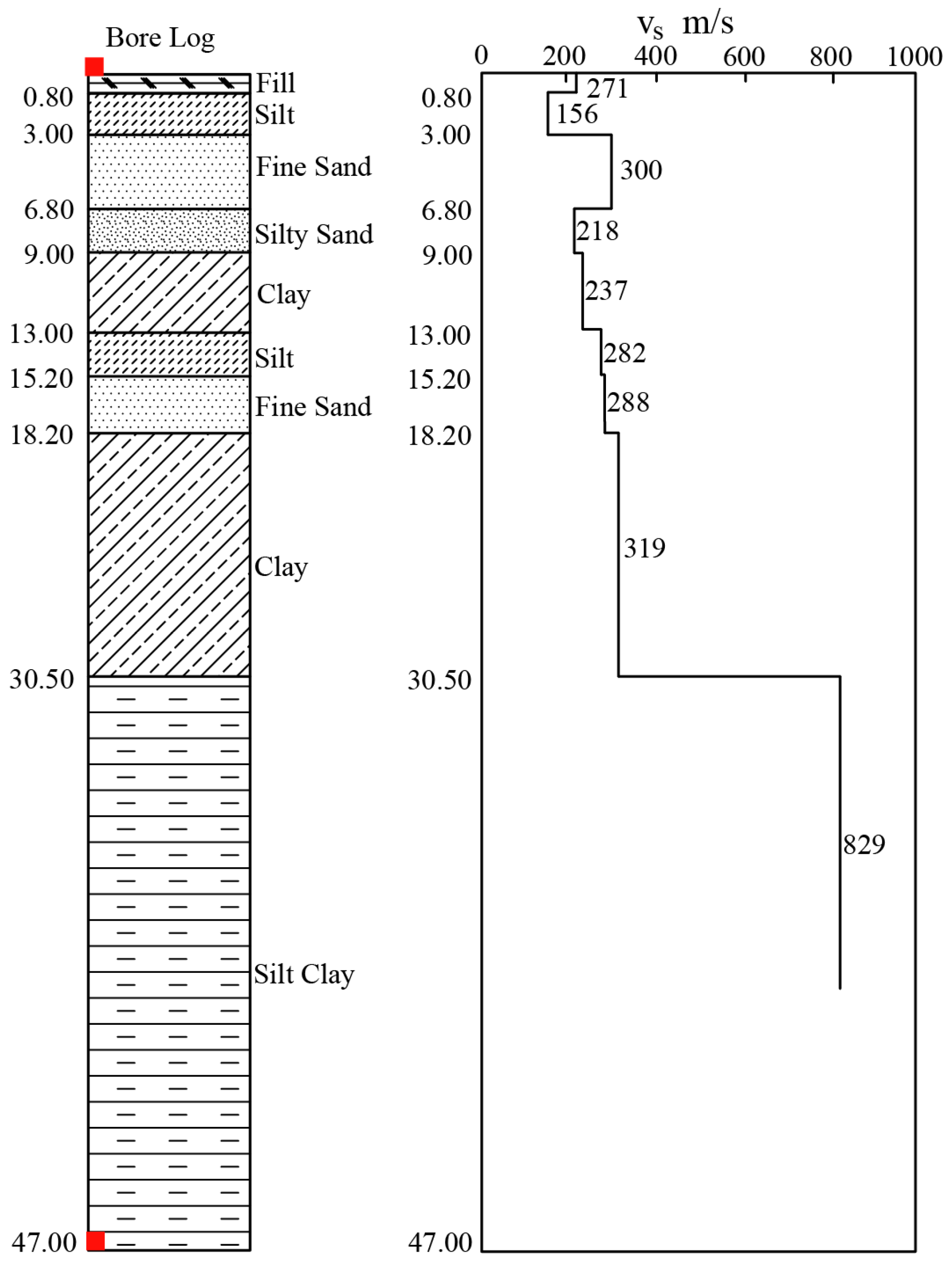
The Xiangtang 3D array, constructed by the China Earthquake Administration, is specifically designed to measure the amplification and attenuation effects of local site conditions on seismic waves, providing strong-motion records at both the bedrock and surface within the same borehole. The array consists of three stations: a bedrock outcrop (Station 1), a borehole with observation points at the surface, 16 m depth, and 32 m depth (Station 2), and a borehole with observation points at the surface and 47 m depth (Station 3). In this study, data from Borehole No. 3 are employed for site response validation. Figure 7 presents the borehole log and shear wave velocity profile of this borehole.

The corresponding soil-layer parameters for numerical modeling are listed in

Table 4. Site parameters of the Tangshan Xiangtang array.

No.	Soil Type	Depth (m)	ρ (kg/m3)	vs (m/s)	ν	γr
1	Fill	0.8	1840	271	0.37	0.000161
2	Silt	3.0	1840	156	0.4	0.000235
3	Fine Sand	6.8	1940	300	0.35	0.000311
4	Silty Sand	9.0	1960	218	0.38	0.000404
5	Clay	13.0	1870	237	0.37	0.000219
6	Silt	15.2	2080	282	0.34	0.000235
7	Fine Sand	18.2	1940	288	0.36	0.000322
8	Clay	30.5	1980	319	0.35	0.000183
9	Silty Clay	-	2070	829	0.33	-

Note: Layer 9 consists of silty clay that is highly weathered.

, obtained from in situ borehole tests and laboratory geotechnical experiments. The dynamic shear modulus reduction curves and damping ratio curves for each soil layer are provided in

Table 5. The relationship between dynamic shear modulus ratio, damping ratio and shear strain of different soil samples.

Soil Type	Sampling Depth (m)	Parameter	Shear Strain γ
			5 × 10−6	1 × 10−5	5 × 10−5	1 × 10−4	5 × 10−4	1 × 10−3	5 × 10−3	1 × 10−2
Fill	0.3–0.5	G/Gmax	0.970	0.941	0.763	0.616	0.243	0.138	0.031	0.016
		λ	0.016	0.029	0.051	0.066	0.098	0.105	0.112	0.113
Silt	1.0–1.2	G/Gmax	0.979	0.959	0.825	0.702	0.320	0.190	0.045	0.023
		λ	0.004	0.007	0.022	0.033	0.065	0.074	0.085	0.087
Silty Sand	3.8–4.0	G/Gmax	0.980	0.960	0.828	0.707	0.326	0.190	0.046	0.026
		λ	0.012	0.017	0.035	0.045	0.037	0.073	0.079	0.080
Silty Sand	7.8–8.0	G/Gmax	0.988	0.976	0.890	0.801	0.447	0.288	0.075	0.039
		λ	0.011	0.015	0.032	0.044	0.074	0.084	0.096	0.097
Clay	10.1–10.3	G/Gmax	0.978	0.956	0.814	0.686	0.304	0.179	0.042	0.021
		λ	0.018	0.024	0.047	0.060	0.086	0.093	0.099	0.100
Silt	1.41–14.3	G/Gmax	0.979	0.996	0.825	0.703	0.321	0.191	0.045	0.023
		λ	0.004	0.007	0.029	0.049	0.106	0.125	0.146	0.149
Fine Sand	16.0–16.2	G/Gmax	0.985	0.970	0.866	0.763	0.392	0.244	0.061	0.031
		λ	0.007	0.011	0.027	0.038	0.067	0.077	0.087	0.089
Clay	27.5–27.7	G/Gmax	0.973	0.948	0.785	0.646	0.268	0.155	0.035	0.018
		λ	0.018	0.024	0.049	0.062	0.088	0.095	0.101	0.102
Silty Clay	—	G/Gmax	1.000	1.000	1.000	1.000	1.000	1.000	1.000	1.000
		λ	0.000	0.000	0.000	0.000	0.000	0.000	0.000	0.000

, derived from dynamic triaxial tests. The reference shear strain γ_r for each layer in Table 4 is obtained by fitting the corresponding modulus reduction curves in Table 5.

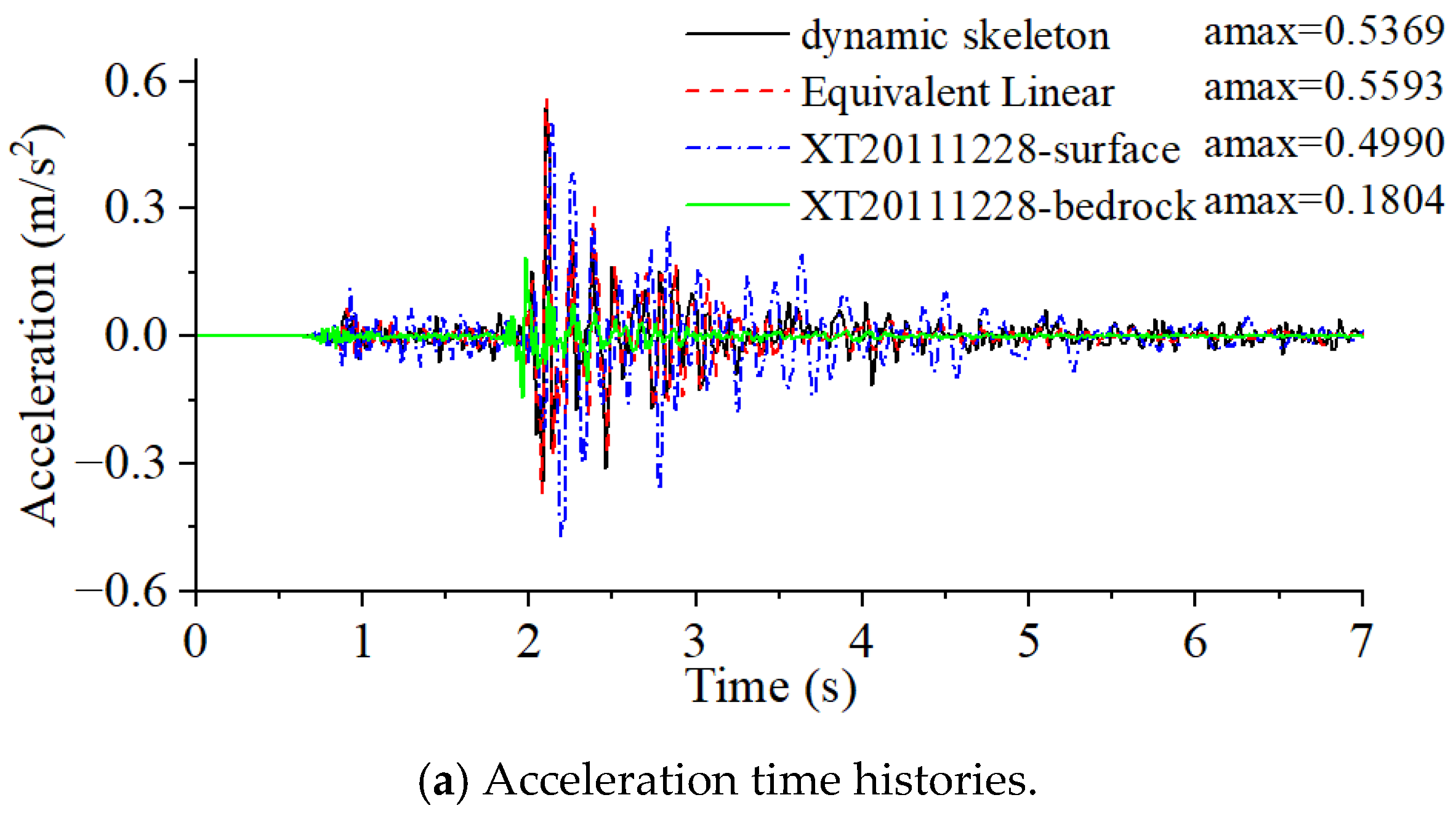
The EW component of the bedrock ground motion recorded at XT20111228 is adopted as the incident wave and is assumed to propagate vertically upward from the bottom of the model. Figure 8a presents the bedrock input motion and a comparison of surface acceleration time histories obtained using the proposed method, the equivalent-linear method, and the measured surface strong-motion records. The peak ground acceleration (PGA) predicted by the proposed method is consistent with both the recorded data and the results from the equivalent-linear method. 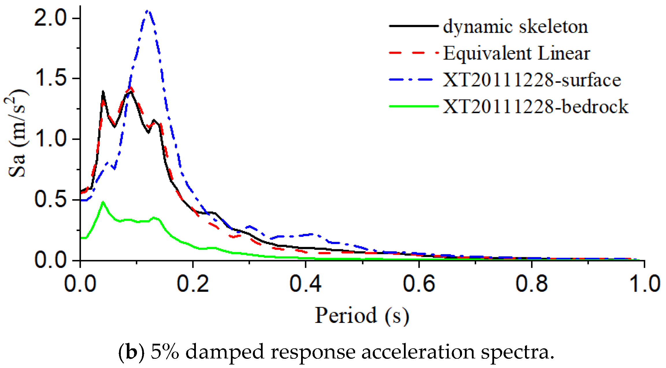Figure 8b presents a comparison of the response spectra. The response spectra obtained using the proposed method exhibit close correspondence with those from the equivalent-linear method. This similarity is mainly attributed to the relatively small amplitude of the incident seismic wave, under which the soil response remains close to the equivalent-linear assumption. These results indicate that the proposed method provides reasonable predictions for irregular loading under weakly nonlinear conditions. Nevertheless, discrepancies are still observed between the simulated and recorded surface response spectra, which may be related to the contribution of additional wave fields, such as surface waves, in the measured records.

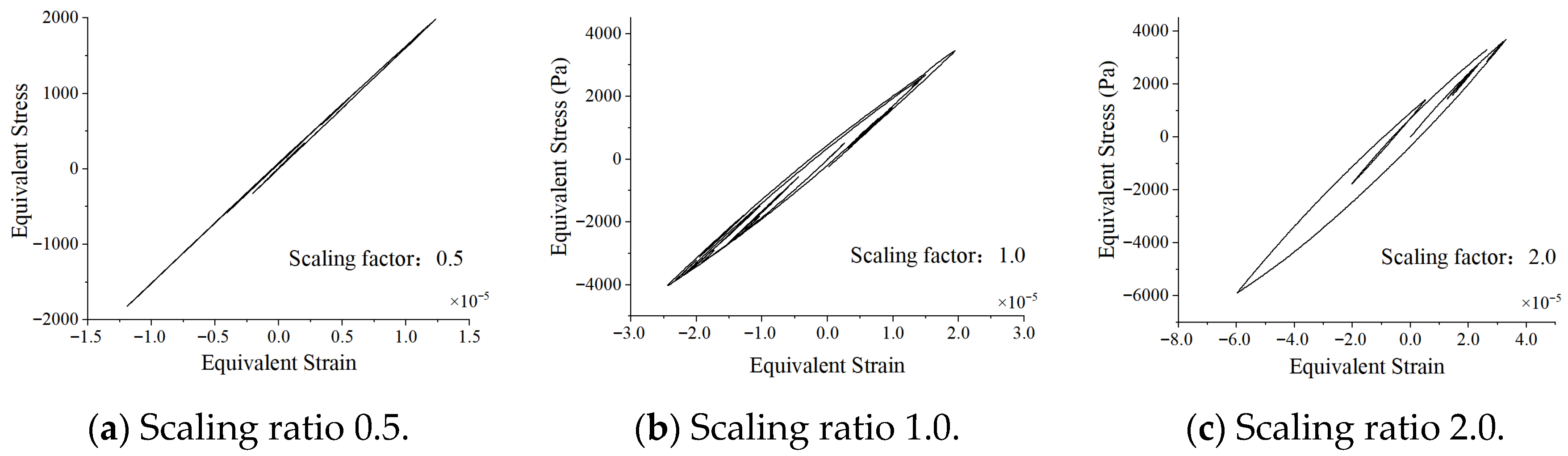
Figure 9 illustrates the stress–strain relationships of the clayey soil layers obtained using the proposed method under different scaling levels of the bedrock motion. With increasing scaling factors, the stress–strain amplitude of a given soil layer increases, and the hysteresis loops become progressively fuller, indicating enhanced energy dissipation in the soil. These observations demonstrate that the proposed method can effectively capture the nonlinear response of soil as the seismic motion amplitude increases.

It should be noted that the validation in this study follows a hierarchical strategy. The Xiangtang array case aims to examine the nonlinear hysteretic behavior of the model under irregular earthquake excitations. The large-strain behavior has been directly verified through element-scale shear tests in Section 3.1. Together, the small-strain site validation and the large-strain element tests support the model’s applicability to the complex loading–unloading scenarios involved in fault rupture analysis.

3.4. Quasi-Static Rupture Propagation

3.4.1. Reverse-Fault Case

To verify the reliability of the proposed dynamic analysis method in reproducing the fundamental characteristics of fault rupture extension, simulations are conducted under quasi-static loading conditions. The results are compared with qualitative observations and quantitative relationships reported in classical studies.

A homogeneous soil layer with a width of 150 m and a thickness of 30 m is considered. A fault with dip angles of 45° and 60° is prescribed beneath the soil layer. For each dip angle, both normal-fault and reverse-fault displacements are imposed. The soil material parameters are the same as those used in Section 3.1. Fault displacement is applied in a quasi-static manner until the rupture zone extends through the overlying soil and reaches the ground surface.

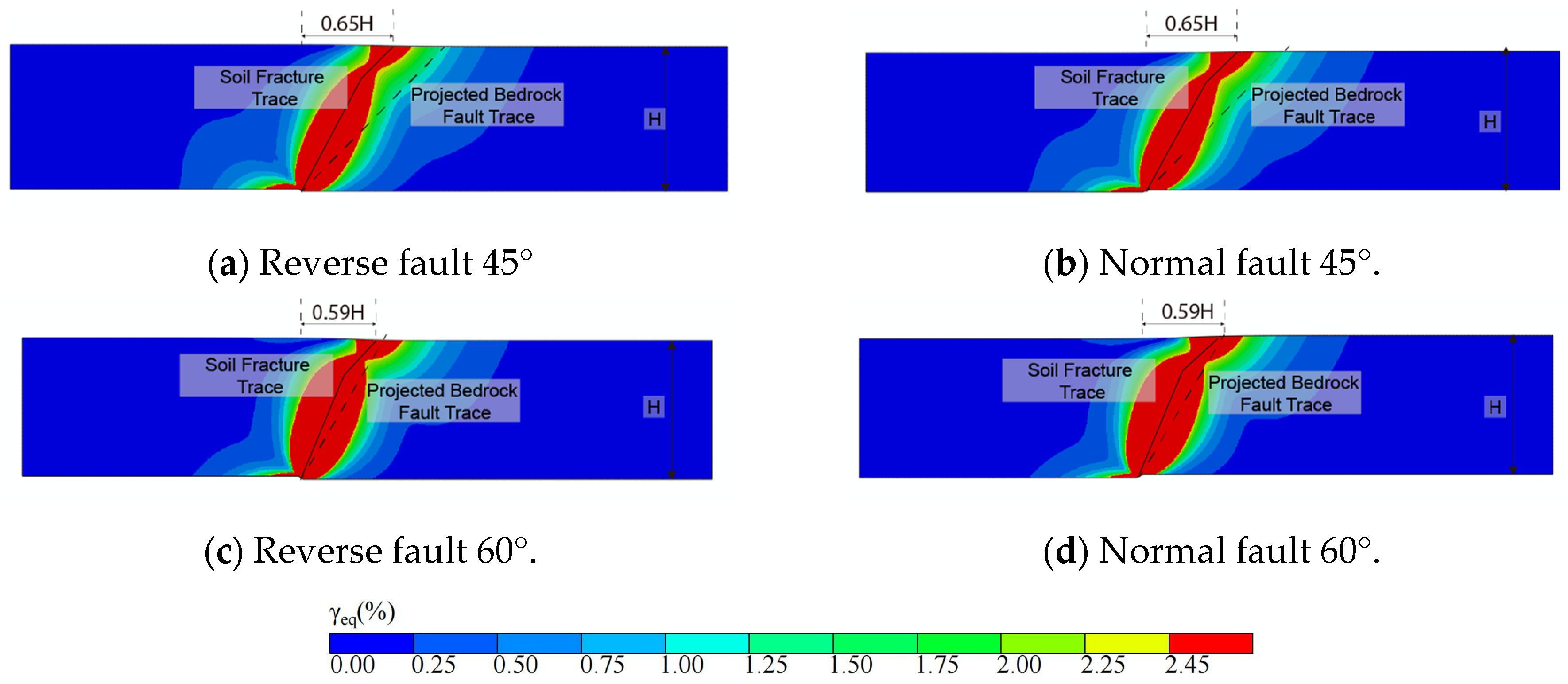
Figure 10 presents the shear band patterns at rupture breakthrough for representative cases. It should be noted that the equivalent shear strain is adopted as an indicator of soil failure in this study. Following the criterion established in our previous work [29] a threshold of 2.45% is selected to identify failure—i.e., elements with equivalent shear strain exceeding 2.45% are interpreted as ruptured. Two main features can be identified. Firstly, when the shear band initiates at the base of the soil layer along the fault, its initial inclination is noticeably larger than the fault dip angle. Secondly, the rupture extension path within the soil layer is nonlinear, exhibiting a deflected trajectory rather than a straight-line extension. These features are qualitatively consistent with centrifuge test observations reported by Bransby, Baziar, and Roth [4,35,36,37], as well as experimental and numerical results reported by Lin and Anastasopoulos [16,38]. This agreement indicates that the proposed method can capture the key geometric characteristics of fault rupture extension in soil layers.

The horizontal distance P is defined as the distance between the location of maximum surface deformation and the vertical projection of the fault onto the ground surface. This distance is further normalized by the soil thickness H. For both normal and reverse faults with a dip angle of 45°, P/H ≈ 0.65, while for a dip angle of 60°, P/H ≈ 0.59. These values are compared with the empirical relationship for surface rupture location summarized by Loukidis et al. [14]:

$$P/H=1.7(1-\beta /90°)\pm 0.3$$

(13)

The empirical formula predicts P/H = 0.85 ± 0.3 for β = 45° and P/H = 0.57 ± 0.3 for β = 60°. The results obtained in this study fall within the allowable range. This agreement indicates that the proposed method provides reasonable estimates of the central location of the fault-induced surface deformation zone.

It should be noted that two simplifications are adopted in this verification. Firstly, the dynamic skeleton curve constitutive model accounts for stiffness degradation and energy dissipation under cyclic loading but neglects the initial geostatic stress field. Consequently, differences between normal-fault and reverse-fault responses are subdued, and features such as graben formation are not reproduced. Secondly, plastic softening after element failure is not considered, resulting in relatively wide high-strain zones and thus an overestimation of the deformation width. From an engineering safety perspective, this overestimation can be regarded as conservative.

In summary, despite the above simplifications, the proposed method reproduces the key geometric characteristics of fault rupture extension, including the curved rupture path in the overlying soil and the quantitative relationship between the surface rupture location and the fault dip angle. These results provide a reliable basis for subsequent analyses of rupture behavior under dynamic loading.

3.4.2. Strike-Slip Fault Case

To validate the capability of the proposed three-dimensional quasi-static strike-slip fault simulation method in reproducing the surface deformation-zone pattern and the along-strike distribution of surface offset, the strike-slip fault model tests by Peng et al. [39] are adopted as a benchmark. The case with a vertical (90°) fault and a 10 cm thick overlying soil is numerically reproduced, and the simulated surface deformation pattern and the along-strike variation in offset are compared with the experimental observations.

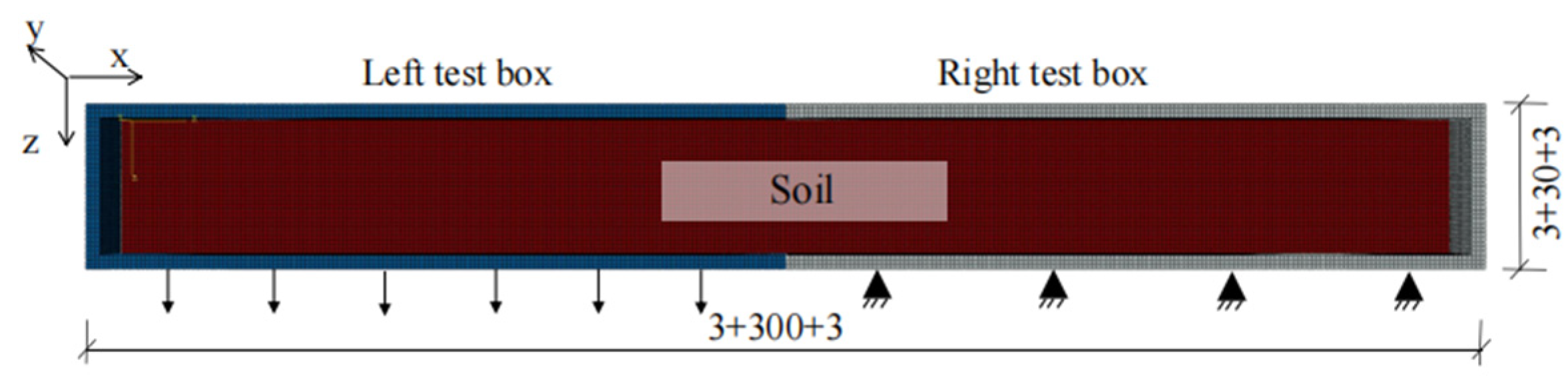
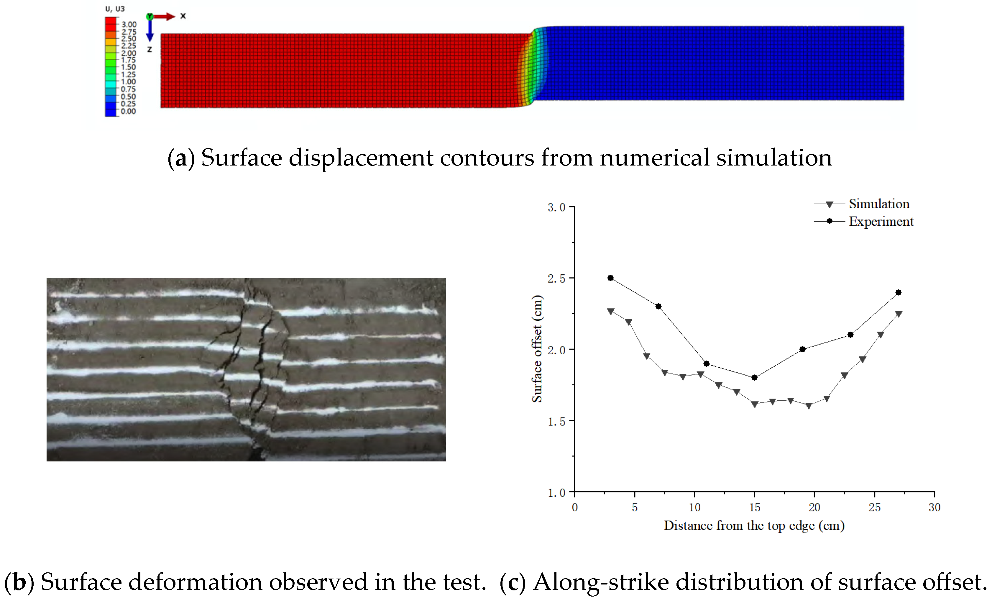
As shown in Figure 11, a three-dimensional model with a homogeneous overlying soil layer is established with dimensions of 300 cm × 30 cm × 10 cm. A test box is further included to match the experimental boundary conditions as closely as possible. Quasi-static loading is applied by fixing one side of the box while imposing a total relative displacement of 3 cm in the z-direction (strike-slip direction) on the other side, thereby producing a typical strike-slip faulting process. To account for the confinement induced by the box walls, frictional contact is adopted between the soil and the box, with a friction coefficient of 0.7. A frictionless contact is specified between the two box halves, representing the experimental condition in which relative sliding between the halves is allowed and the interfacial shear resistance is negligible. Material parameters of the soil layer and the model box are listed in

Table 6. Material parameters of the soil layer and model box for the verification model.

Soil Type	ρ (kg/m3)	vs (m/s)	Gmax (Pa)	ν	γr
Sand	1520	73	8.0 × 106	0.3	0.001
Test box	7850	3130	7.7 × 1010	0.3	/

.

To compare the surface deformation patterns, the surface displacement contours after imposing the 3 cm slip are extracted (Figure 12a) and compared with the surface deformation observed by Peng et al. [39] after loading and a 24 h rest period (Figure 12b). The results show that the simulated deformation-affected zone agrees well with the test in terms of plan-view geometry and along-strike continuity. The band-shaped shear deformation zone induced by a shallow-buried vertical strike-slip fault is well reproduced, indicating that the proposed method provides a reasonable prediction of the rupture-zone geometry.

The along-strike distribution of surface offset is further examined (Figure 12c). The maximum and minimum offsets obtained in this study are approximately 2.3 cm and 1.6 cm, slightly smaller than the experimental values of 2.5 cm and 1.8 cm. However, the along-strike variation trend is consistent with the test results, capturing the key feature that the offset is not uniform along the strike. This amplitude discrepancy is mainly attributed to the viscoelastic constitutive model adopted herein, which does not include potential failure mechanisms in the experimental sand (e.g., plastic yielding and dilatancy). Without pronounced strain localization, the imposed slip tends to be accommodated by distributed shear deformation over a wider zone, leading to less concentrated relative sliding and hence a smaller surface offset. Since this section focuses on the reproducibility of the fundamental characteristics of strike-slip-induced surface deformation, the above discrepancy does not affect the reliability assessment of the proposed method.

It should be noted that, because the displacement field is smoother in the numerical model, directly taking a single-point displacement jump on the fault trace may be sensitive to mesh discretization and local distortion and may not be strictly equivalent to the experimentally measured “offset at the fault line.” To improve comparability, the surface offset is defined as the difference in z-direction displacement between two surface nodes located at +/− one element length from the geometric centerline of the surface deformation zone.

4. Dynamic Rupture Analysis of Different Fault Types

Based on the method developed and validated above, this study selects representative rupture scenarios for a typical reverse fault and a strike-slip fault, and performs a comparative investigation between dynamic explicit analyses and quasi-static analyses. The objective is to clarify how dynamic effects relative to the cumulative slip influence the evolution of overlying soil rupture and to identify the primary dimensions in which these effects manifest.

4.1. Numerical Model for Strike-Slip Faulting

A representative strike-slip fault site with an overlying soil layer is modeled to compare three-dimensional dynamic explicit and quasi-static simulations. The objective is to evaluate whether the proposed approach can reproduce the full rupture sequence in the overlying soil (initiation–propagation–connection–stabilization) and to assess the role of dynamic effects (inertia and stress-wave propagation/superposition) relative to cumulative fault slip.

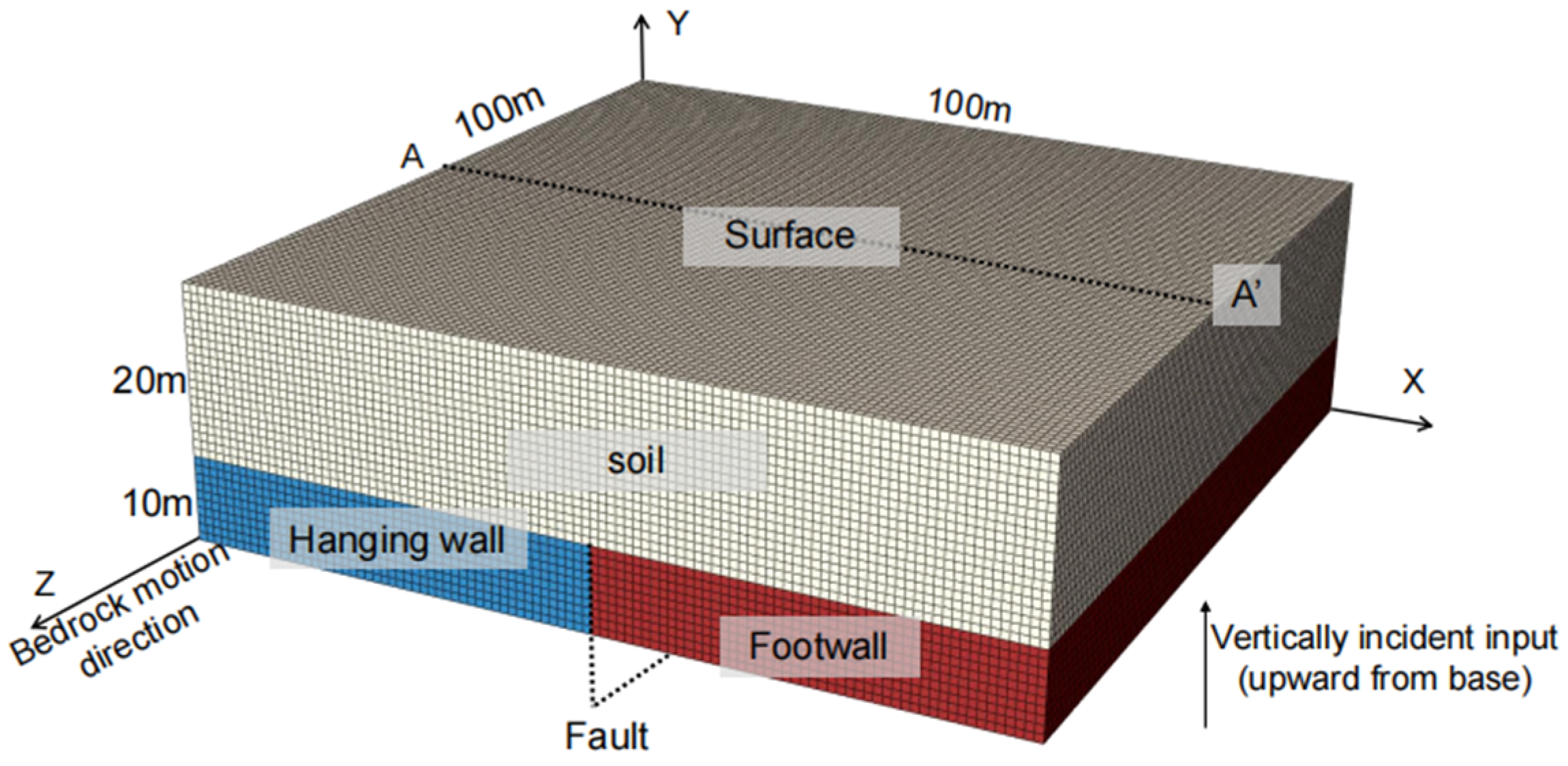
As illustrated in Figure 13, the model measures 100 m × 100 m × 30 m and consists of a 20 m thick soil layer overlying 10 m of bedrock. A vertical strike-slip fault is embedded in the bedrock, dividing it into two blocks; bedrock motion is parallel to the fault strike (z-direction). Viscoelastic boundaries are applied on the four lateral sides and the bottom. A representative fault-normal section (AA′) through the model center is used to extract surface displacement profiles for comparison. The material parameters adopted for both the overlying soil layer and the bedrock are summarized in

Table 7. Model material parameters.

Soil Type	ρ (kg/m3)	vs (m/s)	Gmax (Pa)	ν	γr
Sand	2000	340	2.35 × 108	0.3	0.0018
Bedrock	2700	1217	4.0 × 109	0.25	/

. Seismic loading is introduced from the bedrock bottom as vertically incident waves, with equivalent inputs prescribed on the two fault sides to represent differential bedrock motions. A domain-size sensitivity check was performed; extending the model length along strike from 100 m to 150 m produces essentially unchanged rupture behavior and surface-slip profiles.

In addition, a mesh sensitivity analysis was performed for the strike-slip model to evaluate the influence of mesh resolution. Simulations with mesh sizes of 5 m, 2 m, 1 m, and 0.5 m were compared. The results showed that the main characteristics of rupture geometry and surface deformation were already captured with a mesh size of 1 m. Refining beyond this size primarily led to smoother strain contours near the model boundaries, without altering the key metrics of displacement magnitude or the overall rupture path. These findings indicate that the numerical results are not significantly sensitive to mesh discretization within the tested range, and the adopted mesh density (1 m) offers a reasonable compromise between computational cost and solution accuracy.

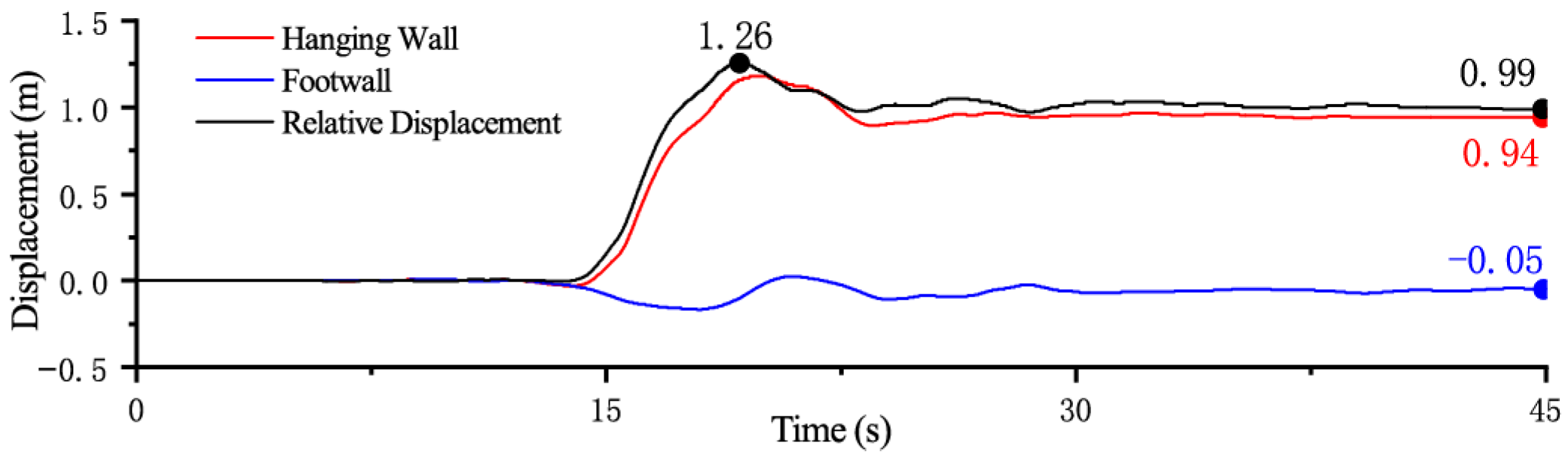
Ground motion records from stations TCU-068 and TCU-103 of the Chi-Chi earthquake are used as input motions (Figure 14). After amplitude scaling, the peak relative fault displacement reaches 1.26 m, and the final residual displacement is 0.99 m. The scaling is implemented for two reasons: (1) to enable a preliminary investigation of the influence of dynamic and quasi-static analysis methods on rupture behavior in the overlying soil, ensuring that the complete rupture evolution—from initiation to stabilization—is captured; and (2) to conduct the quasi-static simulation using the bedrock offset at the end of dynamic analysis, where reducing the permanent displacement improves computational efficiency without compromising comparative accuracy.

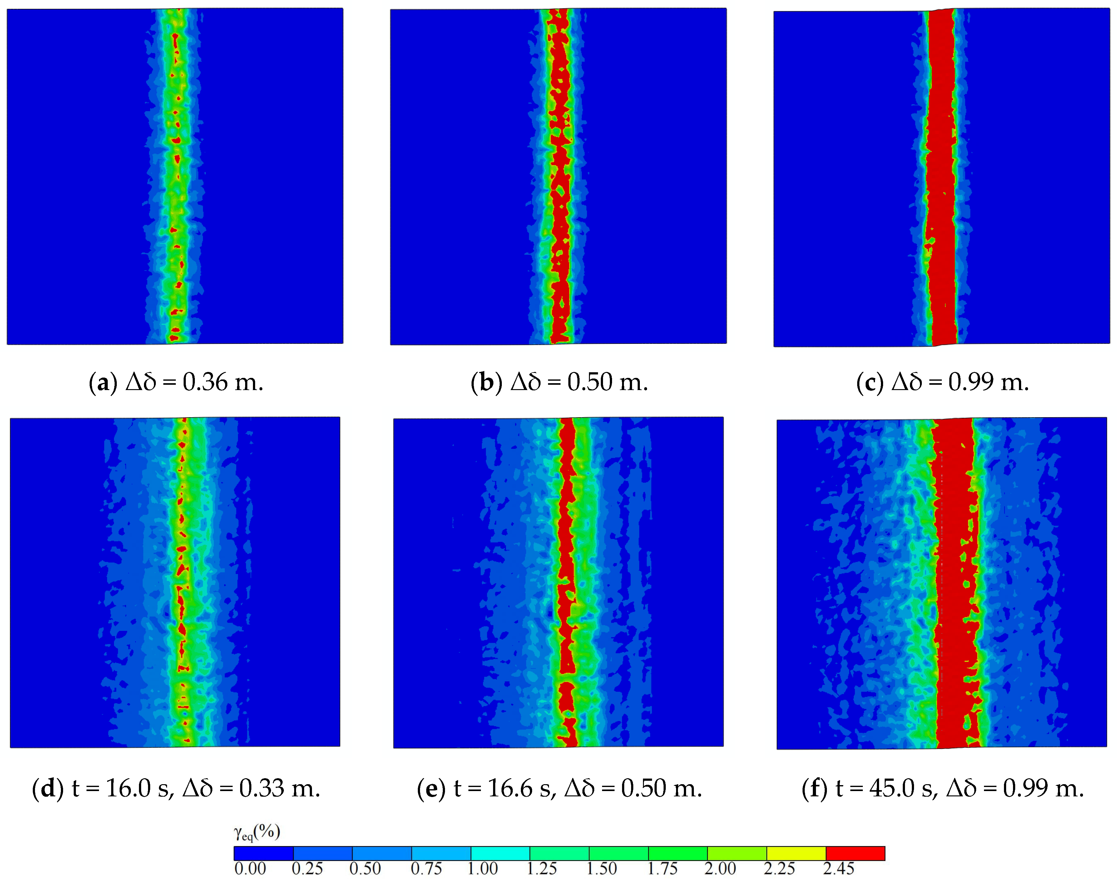
Figure 15 compares surface equivalent-shear-strain contours from the quasi-static and dynamic simulations at three representative stages. Both methods show the same macroscopic evolution: high shear strain first concentrates near the ground surface trace of the bedrock fault, showing a patchy pattern; connectivity increases with accumulating relative bedrock slip; and a continuous high-strain zone eventually forms along the fault strike at the ground surface. The cumulative slip associated with rupture initiation and connection is also very close in the two analyses: in the dynamic simulation, surface rupture initiates at t ≈ 16.0 s (Δδ ≈ 0.33 m), compared with Δδ ≈ 0.36 m in the quasi-static case; rupture connection occurs at Δδ ≈ 0.50 m in both (Figure 14). These results indicate that, for the adopted material parameters and boundary conditions, the initiation and connection thresholds are primarily controlled by cumulative relative slip, with only a minor influence from dynamic effects on the required slip level.

Despite similar thresholds, the dynamic simulation exhibits stronger spatial heterogeneity. At the same cumulative slip, high-strain zones are more patchy and show clearer lateral spreading, consistent with rapid local stress fluctuations induced by wave propagation/reflection/superposition and inertia. In contrast, the quasi-static response, lacking inertia and wave interactions, evolves more smoothly and remains more localized above the fault.

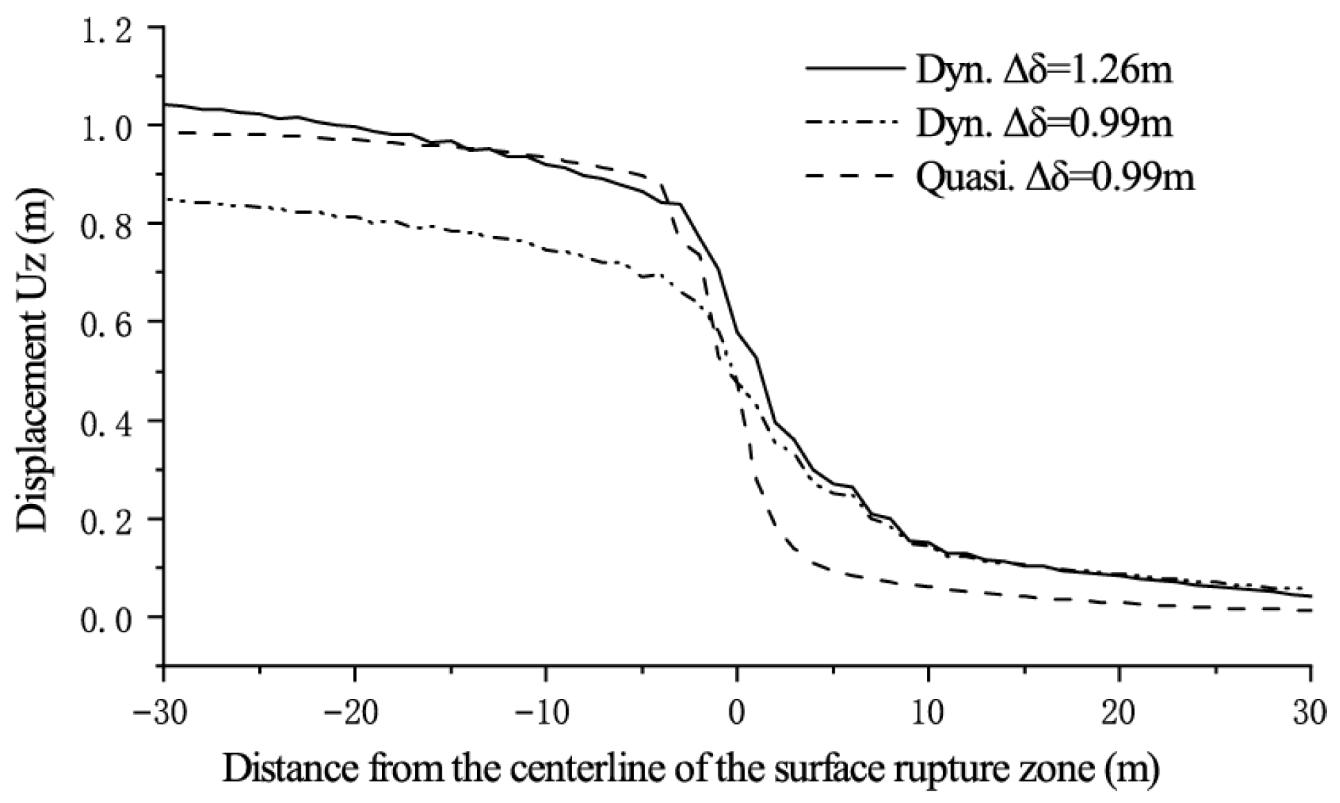
To quantify near-fault surface deformation, Figure 16 presents the z-direction surface displacement along section AA′ within ±30 m of the rupture centerline. At the peak-slip stage, the dynamic response shows markedly larger surface displacement than the quasi-static prediction, highlighting transient amplification. When compared at the same cumulative slip, the dynamic case exhibits a wider influence zone and gentler displacement gradients, indicating reduced near-fault localization relative to the quasi-static case, which shows a sharper gradient and stronger concentration. This suggests that inertia and wave superposition promote short-duration spreading of deformation, producing a broader deformation-affected zone.

4.2. Influence of Dynamic Effects on Overlying Soil Rupture Evolution

Comparisons of the strike-slip case between dynamic and quasi-static simulations show that quasi-static simulations robustly capture the final deformation localization and rupture-zone geometry driven by permanent slip, whereas dynamic simulations further reveal the time-dependent rupture process and transient responses associated with inertia and wave propagation. The two approaches are consistent in macroscopic rupture patterns, but differ systematically in threshold sensitivity, peak response, and the spatial extent of deformation.

First, the influence of dynamic effects on initiation and connection thresholds depends on faulting mechanism and parameter combinations. In the strike-slip case studied here, the initiation and connection slips are nearly identical between dynamic and quasi-static analyses, indicating dominant control by cumulative slip. Overall, for the initiation and connection thresholds considered here, quasi-static analysis is generally adequate because they are primarily controlled by cumulative slip; dynamic analysis is mainly needed to resolve transient amplification.

Second, dynamic analysis captures transient peak amplification that may not be reflected in the final permanent deformation, even when the quasi-static and dynamic residual offsets are similar. This is critical for assessing maximum demand and short-term limit states of fault-crossing structures.

Finally, in terms of spatial patterns, dynamic loading tends to produce migrating and widening zones of intense surface deformation, with a more patchy localization pattern. This behavior arises because stress-wave propagation, reflection, and superposition drive rapid fluctuations in the local stress state, while inertia further amplifies the non-uniform evolution of deformation. By contrast, quasi-static analysis does not capture wave-induced stress fluctuations; deformation is therefore governed primarily by slip accumulation, and the rupture zone evolves more smoothly and remains more localized.

Consequently, dynamic simulation is needed when rupture timing, peak response, and an upper bound of the deformation-affected zone are of interest.

5. Conclusions

This paper presents a full-process numerical method for simulating the initiation and evolution of rupture in overlying soils induced by dynamic fault slip. The proposed method integrates a two-sided, non-uniform wave-input technique based on viscoelastic artificial boundaries with an improved dynamic backbone-curve constitutive model that captures soil nonlinearity and shear failure. The ABAQUS VUMAT implementation reproduces the nonlinear stress–strain response and shear-failure behavior of soils, and its correctness and applicability are supported by verification studies including element-level cyclic shear tests, irregular-loading response of a level-ground site, and the reproduction of quasi-static rupture patterns.

Comparisons between dynamic and quasi-static results demonstrate that inertia and stress-wave propagation/superposition modify the spatiotemporal evolution of rupture, and can induce transient amplification of peak surface displacement as well as migration and widening of the deformation-affected zone. Accordingly, relying solely on quasi-static analysis may underestimate peak-deformation demand and the upper bound of the affected zone.

Overall, quasi-static analysis is efficient for evaluating permanent offset and the final rupture-band location, whereas full dynamic simulation is necessary for resolving rupture sequencing, assessing peak-deformation risk, and providing conservative estimates of the maximum deformation-affected zone. The proposed method provides a reliable numerical tool for seismic safety assessment of fault-crossing infrastructure, and can be further extended to incorporate structural elements such as foundations and tunnels to analyze their influence on fault rupture propagation and surface deformation for more targeted engineering risk assessment.