Variational Bayesian-Based Reliability Evaluation of Nonlinear Structures by Active Learning Gaussian Process Modeling

Abstract

In this study, variational Bayesian inference (VBI) with Gaussian mixture models is applied to update models of nonlinear structures, and then, the calibrated model is employed to estimate the failure probability of structures using a subset simulation (SS) algorithm. To improve the computation efficiency of probabilistic nonlinear model updating, a Gaussian Process (GP) model is used to construct a surrogate likelihood function in Bayesian inference using an active learning algorithm, and then, Gaussian mixture models (GMMs) are employed to approximate the unknown posterior probabilistic density functions (PDFs) of model parameters. The optimized hyperparameters of GMMs can be obtained by maximizing the evidence lower bound (ELBO), and the stochastic gradient search method is used to solve this optimization problem. Based on the optimized hyperparameters, the posterior distributions of model parameters can be approximated using a combination of multiple Gaussian components. Subsequently, the SS algorithm is used to calculate the earthquake-induced failure probability of structures based on the calibrated nonlinear model. To verify the feasibility and effectiveness of the proposed method, a numerical simulation of a two-span bridge structure subjected to seismic excitations was developed. Moreover, the proposed strategy is further applied to estimate the failure probability of a scaled monolithic column structure subjected to bi-directional earthquake excitations. Both numerical and experimental results indicate that the proposed method is feasible and effective for probabilistic nonlinear model updates, and the updated model can significantly enhance the accuracy of structural failure probability predictions.

1. Introduction

Due to harsh environmental conditions, civil structures will unavoidably experience environmental erosion and strong loading excitations during their service life. Under these circumstances, structural performance may degrade and their load-carrying capacity may decrease, especially when subjected to extreme loading conditions, i.e., earthquakes and typhoons [1,2,3]. Cutting-edge sensor technologies and monitoring approaches must be used to evaluate structural reliability and safety performance [4,5]. An accurate finite element (FE) model can provide a significant basis for structural health monitoring, damage assessment, and safety evaluation [6,7]. However, in real applications, an FE model built around only design documents often exhibits significant discrepancies from real structures, which may be caused by idealized boundary conditions, inaccuracies in material constitutive models, and the existence of material and geometric parameter errors [8]. Under these circumstances, some advanced model-updating approaches have been developed to calibrate the initial parameters of structural FE models, which can improve model prediction accuracy and reduce the discrepancy between FE models and real structures.

In nonlinear model-updating studies [9,10], the proposed approaches primarily consist of two types: deterministic and probabilistic model updating. However, since deterministic nonlinear model-updating strategies overlook the influence of uncertainty factors, optimized calibration results only represent one of their potential uncertainty models. Consequently, they may not adequately capture the nonlinear behavior of real-world structures subjected to seismic excitations. To consider the effects of uncertainty factors in model updating, such as measurement noise, modeling error, and structural element discretization, probabilistic nonlinear model-updating techniques have been widely investigated by some scholars [11,12,13,14]. In the above approaches, Bayesian inference has emerged as a dominant approach due to the following advantages: (1) it provides a comprehensive framework for integrating prior knowledge with observed data; (2) the calibrated model parameters are specified by probability distributions, which can enhance the robustness and accuracy of model predictions [15,16]. For instance, Ding et al. [16] used the instantaneous parameters of decomposed components from structural dynamic responses to construct a likelihood function, and the posterior PDFs of model parameters were estimated using the delayed rejection adaptive Metropolis–Hastings sampling algorithm. In addition, Pandey et al. [17] developed a revised likelihood function in a Bayesian inference framework based on the statistics of measured backbone curves, and the posterior distributions of nonlinear system parameters were estimated using the Markov Chain Monte Carlo (MCMC) sampling algorithm. Moreover, Ramancha et al. [18] investigated the identifiability of nonlinear model parameters and subsequently implemented model updating for complex nonlinear structures based on Bayesian inference, and the posterior PDF of model parameters was estimated using a transitional MCMC sampling method. Additionally, the hierarchical Bayesian modeling framework was constructed for the stochastic nonlinear model updating of two Bouc–Wen hysteresis systems using time history data [19], and the investigation results indicated that the method was reliable for the parameter identification and uncertainty quantification of hysteresis-type nonlinear models.

However, although the above-mentioned approaches have been successfully applied for the probabilistic nonlinear model updating of structures, the computational cost remains a challenge when applying these approaches for the model updating of complex and large-scale structures [20,21]. To reduce the computational burden of using Bayesian inference for parameter identification in high-dimensional parameter space, some approximate Bayesian inference methods [22,23] have been developed. For instance, in research on approximate Bayesian methods, some scholars have proposed using variational inference for the posterior distribution estimation of system parameters in complex nonlinear systems. The method transforms the estimation of posterior probabilistic density functions (PDFs) of parameters into an optimization problem, significantly reducing computational complexity for parameter uncertainty quantification and providing a novel framework for the probabilistic model updating of complex structural systems. For instance, Ni et al. [24] proposed using a variational inference strategy for the probabilistic model updating of structures, and the updated model was then used for structural damage detection. Moreover, Li et al. [25] employed the variational Gaussian copula model to solve parameter dependencies in probabilistic model updating, and the feasibility and effectiveness of the proposed approach were validated with two types of civil structures. Hong et al. [26] developed a revised VBI approach for the posterior PDF approximation of unknown model parameters based on observation data. In this study, two types of Bayesian numerical methods, including Bayesian optimization and Bayesian quadrature approaches, were employed to improve computational efficiency for the posterior estimation of model parameters.

Therefore, to improve the accuracy of structural reliability evaluation, in this study, variational Bayesian inference (VBI) with Gaussian mixture models (GMMs) was employed for the probabilistic model updating of nonlinear structures based on structural dynamic responses. Then, the calibrated nonlinear model was used for structural failure probability estimation using the SS algorithm. In variational inference, the active learning Gaussian Process (GP) model is used to construct the surrogate likelihood function for joint probability distribution estimation. Compared to the traditional GP model, it can significantly reduce computational cost for training sample generation, especially for complex engineering structures [27,28,29]. Since the most informative samples are added to the training set for surrogate model optimization at each iteration, it can improve the convergence performance of variational parameters. To verify the feasibility and effectiveness of the proposed method, a numerical simulation of a two-span continuous rigid-frame bridge subjected to seismic excitations was developed. Moreover, a scaled segmental column shake table structure subjected to bi-directional earthquake excitations was experimentally investigated. There are two primary contributions of this study: (1) An active learning GP model was employed to construct the surrogate likelihood function in variational inference, which can avoid the time-consuming nonlinear dynamic analysis in training sample generation. (2) By combining probabilistic nonlinear model updating with the SS algorithm, the calculated failure probability of structures is more reliable than those based on prior knowledge of model parameters.

2. Theoretical Background

2.1. The Basic Theory of VBI

VBI is an approximation strategy in Bayesian statistics and machine learning used to tackle problems where traditional Bayesian inference is computationally intractable, and it approximates the true posterior distribution of structural parameters using tractable probabilistic models [30]. The approach transforms the complex posterior PDF calculation of structural parameters into a hyperparameter optimization problem, which can significantly improve computational efficiency in parameter estimation, particularly for large datasets and complex structural models.

Referring to previous studies [31] and assuming the model parameter vector of a nonlinear structure is $\mathit{\theta }$, the posterior PDFs of these parameters under observed data $\mathit{Y}$ are denoted as $p\left(\mathit{\theta }\right|\mathit{Y})$. In classic Bayesian inference, $p\left(\mathit{\theta }\right|\mathit{Y})$ can be evaluated using Equation (1):

$$p\left(\mathit{\theta }\right|\mathit{Y})\propto cp\left(\mathit{Y}\right|\mathit{\theta })p\left(\mathit{\theta }\right)$$

(1)

where c denotes a normalization constant, and $p\left(\mathit{\theta }\right)$ and $p\left(\mathit{Y}\right|\mathit{\theta })$ correspond to the prior distribution of model parameters and likelihood function, respectively. The posterior PDFs of model parameters can typically be estimated via maximum likelihood estimation or using stochastic sampling algorithms [31,32]. However, computational cost remains an issue for parameter estimation in high-dimensional spaces [33].

To improve computational efficiency for the posterior estimation of high-dimensional parameter vectors, in this study, the VBI method was applied to solve this issue. Before using the VBI method to calculate $p\left(\mathit{\theta }\right|\mathit{Y})$, a series of tractable probabilistic models, marked as $q_{\varphi }\left(\mathit{\theta }\right)$, can be employed to approximate the posterior PDFs of model parameters. Based on previous studies [34], typical probability distributions such as the normal, multivariate Gaussian, and Gamma distributions are generally applicable. In this study, the posterior distributions of nonlinear model parameters are approximated using GMMs, which can be written as

$$q_{\varphi }\left(\mathit{\theta }\right)={\sum }_{i=1}^l{\tau }_{i}N\left(\mathit{\theta };{\mu }_i;{\sigma }_i^2\Sigma \right)$$

(2)

where $N\left(\mathit{\theta };{\mu }_i;{\sigma }_i^2\Sigma \right)$ denotes the ith Gaussian component of the defined GMM, characterized by its mean vector ${\mu }_i$ and scale ${\sigma }_i$; ${\tau }_i$ is the weight coefficient of the ith component, whose feasible range is between 0 and 1, and the sum of all coefficients ${\tau }_i$ equal to 1; and $\Sigma$ is a diagonal covariance matrix, denoted as $\Sigma =diag\left(\left[{\beta }_1^2,{\beta }_2^2,\cdots ,{\beta }_D^2\right]\right)$ (D is the number of unknown model parameters). The approximate probability distribution of $q_{\varphi }\left(\mathit{\theta }\right)$ can be parameterized as $\varphi =({\tau }_1,{\tau }_2,\cdots ,{\tau }_l,{\mu }_1,{\mu }_2,\cdots ,{\mu }_l,{\sigma }_1,\cdots ,{\sigma }_l,{\beta }_1,{\beta }_2,\cdots ,{\beta }_D)$.

Referring to the previous studies [35], the log marginal probability in Bayesian inference can be expressed as

$$\begin{array}{cc}\hfill \mathrm{l}\mathrm{o}\mathrm{g}p\left(\mathit{Y}\right)& =\mathrm{l}\mathrm{o}\mathrm{g}{\displaystyle \frac{p\left(\mathit{Y}\right|\mathit{\theta })p\left(\mathit{\theta }\right)}{p\left(\mathit{\theta }\right|\mathit{Y})}}=\int q_{\varphi }\left(\mathit{\theta }\right)\mathrm{l}\mathrm{o}\mathrm{g}{\displaystyle \frac{p\left(\mathit{Y}\right|\mathit{\theta })p\left(\mathit{\theta }\right)}{p\left(\mathit{\theta }\right|\mathit{Y})}} {\displaystyle \frac{q_{\varphi }\left(\mathit{\theta }\right)}{q_{\varphi }\left(\mathit{\theta }\right)}} d\mathit{\theta }\hfill \\ \hfill & =\int q_{\varphi }\left(\mathit{\theta }\right)\left(\mathrm{l}\mathrm{o}\mathrm{g}{\displaystyle \frac{p\left(\mathit{Y}\right|\mathit{\theta })p\left(\mathit{\theta }\right)}{q_{\varphi }\left(\mathit{\theta }\right)}}+\mathrm{l}\mathrm{o}\mathrm{g}{\displaystyle \frac{q_{\varphi }\left(\mathit{\theta }\right)}{p\left(\mathit{\theta }\right|\mathit{Y})}}\right) d\mathit{\theta }\hfill \\ \hfill & =\int q_{\varphi }\left(\mathit{\theta }\right)\mathrm{l}\mathrm{o}\mathrm{g}{\displaystyle \frac{p\left(\mathit{Y}\right|\mathit{\theta })p\left(\mathit{\theta }\right)}{q_{\varphi }\left(\mathit{\theta }\right)}}d\mathit{\theta }+\int q_{\varphi }\left(\mathit{\theta }\right)\mathrm{l}\mathrm{o}\mathrm{g}{\displaystyle \frac{q_{\varphi }\left(\mathit{\theta }\right)}{p\left(\mathit{\theta }\right|\mathit{Y})}}d\mathit{\theta }\hfill \\ \hfill & =L_E\left[q_{\varphi }\left(\mathit{\theta }\right)\right]+KL\left(q_{\varphi }\left(\mathit{\theta }\right)\Vert p\left(\mathit{\theta }\right|\mathit{Y})\right)\hfill \end{array}$$

(3)

From Equation (3), it is observed that the derivations of $\mathrm{l}\mathrm{o}\mathrm{g}p\left(\mathit{Y}\right)$ consist of two parts: $L_E\left[q_{\varphi }\left(\mathit{\theta }\right)\right]$ and $KL\left(q_{\varphi }\left(\mathit{\theta }\right)\Vert p\left(\mathit{\theta }\right|\mathit{Y})\right)$. Here, $L_E\left[q_{\varphi }\left(\mathit{\theta }\right)\right]$ denotes the ELBO, whose detailed expression can be presented as

$$\begin{array}{cc}\hfill L_E\left[q_{\varphi }\left(\mathit{\theta }\right)\right]=& \int q_{\varphi }\left(\mathit{\theta }\right)\mathrm{l}\mathrm{o}\mathrm{g}{\displaystyle \frac{p\left(\mathit{Y}\right|\mathit{\theta })p\left(\mathit{\theta }\right)}{q_{\varphi }\left(\mathit{\theta }\right)}}d\mathit{\theta }\hfill \\ \hfill & =\int q_{\varphi }\left(\mathit{\theta }\right)\mathrm{l}\mathrm{o}\mathrm{g}\left[p\left(\mathit{Y}\right|\mathit{\theta })p\left(\mathit{\theta }\right)\right]d\mathit{\theta }-\int q_{\varphi }\left(\mathit{\theta }\right)\mathrm{l}\mathrm{o}\mathrm{g}{q}_{\varphi }\left(\mathit{\theta }\right)d\mathit{\theta }\hfill \\ \hfill & =L_1\left[g\left(\mathit{\theta }\right)\right]+L_2\left[q_{\varphi }\left(\mathit{\theta }\right)\right]\hfill \end{array}$$

(4)

where $L_1\left[g\left(\mathit{\theta }\right)\right]$ is the expected value of the log joint probability density function and $L_2\left[q_{\varphi }\left(\mathit{\theta }\right)\right]$ denotes the entropy of $q_{\varphi }\left(\mathit{\theta }\right)$.

In addition, the second term $KL\left(q_{\varphi }\left(\mathit{\theta }\right)\Vert p\left(\mathit{\theta }\right|\mathit{Y})\right)$, presented in Equation (3), is the Kullback–Leibler (KL) divergence, which reflects the discrepancy between the true probability distributions and approximated distributions. In this study, since the main purpose of variational inference is to approximate the true posterior distribution of structural parameters with GMMs, the KL divergence must be minimized between the two types of probability distributions [23]. In addition, as observed in Equation (3), note that the value of KL divergence is a non-negative constant for any approximate distribution $q_{\varphi }\left(\mathit{\theta }\right)$, and the relationship $L_E\left[q_{\varphi }\left(\mathit{\theta }\right)\right]\le \mathrm{l}\mathrm{o}\mathrm{g}p\left(\mathit{Y}\right)$ exists. Therefore, the parameters of approximate posterior distribution $q_{\varphi }\left(\mathit{\theta }\right)$ can be obtained by maximizing the ELBO, which is written as

$${\mathit{\theta }}^{*}=arg \mathrm{m}\mathrm{a}\mathrm{x}{\left\{L_E\left[q_{\varphi }\left(\mathit{\theta }\right)\right]\right\}}_{ELBO}=arg \mathrm{m}\mathrm{a}\mathrm{x}\left\{L_1\left[g\left(\mathit{\theta }\right)\right]+L_2\left[q_{\varphi }\left(\mathit{\theta }\right)\right]\right\}$$

(5)

From Equations (3) and (5), to ensure $L_E\left[q_{\varphi }\left(\mathit{\theta }\right)\right]$ reaches its maximum value, it is necessary to minimize the KL divergence. In this circumstance, the problem of maximizing the ELBO can be transformed into the minimization of the KL divergence between two types of probability distributions, and thus, the parameters of the approximate posterior distribution $q_{\varphi }\left(\mathit{\theta }\right)$ can be identified by minimizing the KL divergence. In variational probability distribution estimation, it is critical to select a reasonable approximate probability distribution for nonlinear parameters, which determines the reliability of the estimated posterior distributions of model parameters. In previous studies [36], GMMs have been used to approximate arbitrary probability distributions by setting appropriate hyperparameters, including the number of Gaussian components, weight coefficients, and mean and covariance matrices of all Gaussian components, and variational inference has been used to optimize the hyperparameters of the GMMs. To overcome high time-consuming computation of joint probability distribution $g\left(\mathit{\theta }\right)$ in variational inference, a GP model was selected for the construction of a surrogate model of $g\left(\mathit{\theta }\right)$ based on an active learning algorithm, and then, $L_1\left[g\left(\mathit{\theta }\right)\right]$ can be efficiently calculated.

2.2. GP Surrogate Model Construction Based on Active Learning Algorithm

In this study, to avoid time-consuming nonlinear dynamic analysis during the iterative optimization of variational parameters, an active learning GP model was used to construct the surrogate likelihood function for joint probability distribution $g\left(\mathit{\theta }\right)$ estimation.

A GP model with a squared exponential kernel [28] can be described as

$$\mathcal{F}\left(\mathit{\theta }\right)=GP\left(m\left(\mathit{\theta }\right),\kappa \left(\mathit{\theta },{\mathit{\theta }}^{\prime }\right)\right)$$

(6)

where $m\left(\mathit{\theta }\right)$ and $\kappa \left(\mathit{\theta },{\mathit{\theta }}^{\prime }\right)$ denote the mean and covariance functions of the GP model, respectively. $\kappa \left(.\right)$ is called the kernel of the GP model, and a squared exponential kernel is used in this study, which can be expressed as

$$\kappa \left(\mathit{\theta },{\mathit{\theta }}^{\prime }\right)={\sigma }_f^2\mathrm{e}\mathrm{x}\mathrm{p}\left(-{\displaystyle \frac{{\Vert \mathit{\theta }-{\mathit{\theta }}^{\prime }\Vert }^2}{2{\lambda }^2}}\right)$$

(7)

Then, the training data, consisting of inputs and outputs, are used to construct the GP surrogate model of $g\left(\mathit{\theta }\right)$. Assume $\widehat{g}\left(\mathit{\theta }\right)$ is the predicted output of the GP model at test point $\mathit{\theta },$ and that it also satisfies the Gaussian distribution. Given the training set $\Theta =\left\{{\mathit{\theta }}_{train}^i,g\left({\mathit{\theta }}_{train}^i\right)\right\}(i=1,2,\cdots ,n_t)$, the distribution of prediction results can be written as

$$\left(\begin{array}{c}g\left({\mathit{\theta }}_{train}\right)\\ \widehat{g}\left(\mathit{\theta }\right)\end{array}\right)~GP\left(\left[\begin{array}{c}m\left({\mathit{\theta }}_{train}\right)\\ m\left(\mathit{\theta }\right)\end{array}\right],\left[\begin{array}{cc}\kappa \left(\Theta ,\Theta \right)+{\widehat{\sigma }}_{obs}^2{\mathit{I}}_{n_t\times n_t}& \kappa {\left(\Theta ,\mathit{\theta }\right)}^T\\ \kappa \left(\mathit{\theta },\Theta \right)& \kappa \left(\mathit{\theta },\mathit{\theta }\right)\end{array}\right]\right)$$

(8)

The probability distribution at point $\mathit{\theta }$ can also be presented as $p_{\widehat{g}}~GP\left(\widehat{g}\left(\mathit{\theta }\right),\widehat{\sigma }\left(\mathit{\theta }\right)\right)$, and the mean value and variance terms can be derived as

$$\widehat{g}\left(\mathit{\theta }\right)=\kappa \left(\mathit{\theta },\Theta \right){\left[\kappa \left(\Theta ,\Theta \right)+{\widehat{\sigma }}_{obs}^2{\mathit{I}}_{n_t\times n_t}\right]}^{-\mathbf{1}}\left(g\left({\mathit{\theta }}_{train}\right)-m\left({\mathit{\theta }}_{train}\right)\right)+m\left(\mathit{\theta }\right)$$

(9)

$$\widehat{\sigma }\left(\mathit{\theta }\right)=\kappa \left(\mathit{\theta },\mathit{\theta }\right)-\kappa \left(\Theta ,\mathit{\theta }\right){\left[\kappa \left(\Theta ,\Theta \right)+{\widehat{\sigma }}_{obs}^2{\mathit{I}}_{n_t\times n_t}\right]}^{-\mathbf{1}}\kappa \left(\mathit{\theta },\Theta \right)$$

(10)

The unknown hyperparameter set of the GP model $\mathit{\Phi }$ can be identified based on training samples. The training process of a GP model can be transformed to maximize the logarithm of the marginal likelihood for the training values.

$$\begin{gathered} \mathit{\Phi }=arg\mathrm{m}\mathrm{a}\mathrm{x} \mathrm{l}\mathrm{o}\mathrm{g}p\left(g\left({\mathit{\theta }}_{train}\right)\right|\mathit{\Phi })=-{\displaystyle \frac{n_t}{2}}log\left(2\pi \right)-{\displaystyle \frac{1}{2}}log\left|\kappa \left(\Theta ,\Theta \right)+{\widehat{\sigma }}_{obs}^2{\mathit{I}}_{n_t\times n_t}\right| \\ -{\displaystyle \frac{1}{2}}{\left(g\left({\mathit{\theta }}_{train}\right)-m\left({\mathit{\theta }}_{train}\right)\right)}^T{(\kappa \left(\Theta ,\Theta \right)+{\widehat{\sigma }}_{obs}^2{\mathit{I}}_{n_t\times n_t})}^{-\mathbf{1}}\left(g\left({\mathit{\theta }}_{train}\right)-m\left({\mathit{\theta }}_{train}\right)\right) \end{gathered}$$

(11)

To improve the convergence performance of variational inference, the active sampling technique was used to optimize the GP model at each iteration. Based on previous studies [29,37], a small number of training samples $\Theta$ are first applied to train the GP model, and then, $n_s$ sets of input–output samples are generated based on the trained GP model, denoted as $\left\{{\mathit{\theta }}_{gen}^i,\widehat{g}\left({\mathit{\theta }}_{gen}^i\right)\right\}(i=1,2,\cdots ,n_s)$. The optimal data points can be identified with the defined active learning function, which is expressed as

$${\left\{{\mathit{\theta }}_{gen}^{*}\right\}}^j=arg\max \psi \left(-{\displaystyle \frac{\left|\widehat{g}\left({\mathit{\theta }}_{gen}^i\right)\right|}{\widehat{\sigma }\left({\mathit{\theta }}_{gen}^i\right)}}\right) \left(j=1,2,\cdots ,n_p\right)$$

(12)

where $\psi \left(·\right)$ represents the cumulative distribution function, and $n_p$ denotes the number of identified best samples. In this study, to balance the computational efficiency and prediction accuracy of variational parameters, $n_p$ was set to 5. In addition, the number of the added sampling points can be appropriately increased when the parameter dimension is higher.

As observed in Equation (12), the maximum value of the active learning function is prone to 1. When the calculated values of the cumulative distribution are larger, the predicted results of the GP model at the corresponding sample points are relatively poor. In this case, it is necessary to add these data samples into the training set to improve the prediction performance of the GP model at the next iteration. The iterative training process of the GP model would terminate when the convergence criteria defined in Section 2.3 are satisfied.

2.3. VBI-Based Probabilistic Nonlinear Model Updating Based on GMMs

2.3.1. The Approximate Calculation Process of ELBO

In Section 2.2, since the joint probability distribution $g\left(\mathit{\theta }\right)$ is characterized by the GP surrogate model, the ELBO and its gradients can be analytically represented and calculated. Accordingly, the entropy of the approximate posterior distribution can be obtained by following the Monte Carlo sampling strategy, and the calculation process can be expressed as

$$L_2\left[q_{\varphi }\left(\mathit{\theta }\right)\right]=-\int q_{\varphi }\left(\mathit{\theta }\right)\mathrm{l}\mathrm{o}\mathrm{g}{q}_{\varphi }\left(\mathit{\theta }\right)d\mathit{\theta }=-{\displaystyle \frac{1}{N_s}}{\sum }_{c=1}^{N_s}{\sum }_{s=1}^l{\tau }_s\mathrm{l}\mathrm{o}\mathrm{g} q\left({\eta }_{m,s}\right)$$

(13)

where ${\eta }_{m,s}={\sigma }_i\mathit{R}{\omega }_{m,s}+{\mu }_i$; $\mathit{R}$ is a diagonal matrix, denoted as $\mathit{R}=diag\left[\beta \right]$; and ${\omega }_{m,s}$ denotes a D-dimensional Gaussian distribution.

Then, the expected value of the log joint PDF can be calculated by

$$\begin{gathered} L_1\left[g\left(\mathit{\theta }\right)\right]=\int q_{\varphi }\left(\mathit{\theta }\right)log\left[p\left(\mathit{Y}\right|\mathit{\theta })p\left(\mathit{\theta }\right)\right]d\mathit{\theta }=\int q_{\varphi }\left(\mathit{\theta }\right)g\left(\mathit{\theta }\right)d\mathit{\theta } \\ ={\sum }_{s=1}^l{\tau }_s\int N\left(\mathit{\theta };{\mu }_s;{\sigma }_s^2\Sigma \right)g\left(\mathit{\theta }\right)d\mathit{\theta }={\sum }_{s=1}^l{\tau }_s{\mathcal{R}}_s \end{gathered}$$

(14)

In Equation (14), considering the term $g\left(\mathit{\theta }\right)$ is represented using the GP-based surrogate model $\widehat{g}\left(\mathit{\theta }\right)$; then, ${\mathcal{R}}_s$ can be derived as

$$\begin{array}{cc}\hfill {\mathcal{R}}_s=& {\displaystyle \int }N\left(\mathit{\theta };{\mu }_s;{\sigma }_s^2\Sigma \right)\widehat{g}\left(\mathit{\theta }\right)d\mathit{\theta }\hfill \\ \hfill & =\int N\left(\mathit{\theta };{\mu }_s;{\sigma }_s^2\Sigma \right)[\kappa \left(\mathit{\theta },\Theta \right){\left[\kappa \left(\Theta ,\Theta \right)+{\widehat{\sigma }}_{obs}^2{\mathit{I}}_{n_t\times n_t}\right]}^{-\mathbf{1}}\left(g\left({\mathit{\theta }}_{train}\right)-m\left({\mathit{\theta }}_{train}\right)\right)]d\mathit{\theta }\hfill \\ \hfill & ={\mathit{z}}_i^T{[\kappa \left(\Theta ,\Theta \right)+{\widehat{\sigma }}_{obs}^2{\mathit{I}}_{n_t\times n_t}]}^{-\mathbf{1}}\left(g\left({\mathit{\theta }}_{train}\right)-m\left({\mathit{\theta }}_{train}\right)\right)+m_0+{\nu }_s\hfill \end{array}$$

(15)

where

$${\nu }_s=-{\displaystyle \frac{1}{2}}{\sum }_{d=1}^D{\displaystyle \frac{1}{{\omega }_d^2}}\left[{\left({\mu }_s^d\right)}^2+{\sigma }_s^2{\lambda }_d^2-2{\mu }_s^d{\theta }_m^d+\left({\theta }_m^d\right)\right]$$

(16)

${\mathit{z}}_s={\left[z_s^1,z_s^2,\cdots ,z_s^r\right]}^T \left(r=1,2,\cdots ,n_t\right)$, and the elements in vector ${\mathit{z}}_s$ are expressed as

$$z_s^r={\sigma }_f^{2}N\left({\mu }_s;{\mathit{\theta }}_{train}^r;{\sigma }_s^2\Sigma +{\Sigma }_l\right)={\displaystyle \frac{{\sigma }_f^2}{{\left(2\pi \right)}^{\frac{D}{2}}{\prod }_j^D\sqrt{{\sigma }_s^2{\lambda }_j^2+l_j^2}}}exp\left(-{\displaystyle \frac{1}{2}}{\sum }_{j=1}^D{\displaystyle \frac{{\left({\mu }_s^j-{\theta }_{train}^{r,j}\right)}^2}{{\sigma }_s^2{\lambda }_j^2+l_j^2}}\right)$$

(17)

The variance of $\eta \left[g\left(\mathit{\theta }\right)\right]$ can be analytically derived by

$${\mathcal{B}}_{\sigma }=\iint q_{\varphi }\left({\mathit{\theta }}_p\right)q_{\varphi }\left({\mathit{\theta }}_q\right)\sigma \left(g\left({\mathit{\theta }}_p\right),g\left({\mathit{\theta }}_q\right)\right)\mathrm{d}{\mathit{\theta }}_{p}d{\mathit{\theta }}_q={\sum }_{s=1}^l{\sum }_{n_c=1}^l{\tau }_s{\tau }_{n_c}{\mathcal{g}}_{s{,n}_c}$$

(18)

where the detailed expression of ${\mathcal{g}}_{is}$ can be written as

$${\mathcal{g}}_{s{,n}_c}=\iint N\left({\mathit{\theta }}_p;{\mu }_s;{\sigma }_s^2\Sigma \right)N\left({\mathit{\theta }}_q;{\mu }_s;{\sigma }_s^2\Sigma \right)\sigma \left(g\left({\mathit{\theta }}_p\right),g\left({\mathit{\theta }}_q\right)\right)\mathrm{d}{\mathit{\theta }}_{p}d{\mathit{\theta }}_q$$

(19)

In addition, the covariance matrix $\sigma \left(g\left({\mathit{\theta }}_p\right),g\left({\mathit{\theta }}_q\right)\right)$ is represented by

$$\sigma \left(g\left({\mathit{\theta }}_p\right),g\left({\mathit{\theta }}_q\right)\right)=\kappa \left({\mathit{\theta }}_p,{\mathit{\theta }}_q\right)-\kappa \left({\mathit{\theta }}_p,\Theta \right){\left[k\left(\Theta ,\Theta \right)+{\widehat{\sigma }}_{obs}^2{\mathit{I}}_{n_t\times n_t}\right]}^{-\mathbf{1}}\kappa \left(\Theta ,{\mathit{\theta }}_q\right)$$

(20)

Therefore, the term ${\mathcal{g}}_{s{,n}_c}$ can be further analytically expressed as

$${\mathcal{g}}_{s{,n}_c}={\sigma }_f^{2}N({\mu }_s;{\mu }_{n_c},{\sum }_l+({\sigma }_f^2+{\sigma }_s^2)\sum )-{\mathit{z}}_s^T{\left[\kappa \left(\Theta ,\Theta \right)+{\sigma }_{obs}^2{\mathit{I}}_{n_t\times n_t}\right]}^{-1}{\mathit{z}}_s$$

(21)

Based on the above derivation process, the ELBO can be analytically calculated using Equations (13) and (14), and then, the hyperparameters of GMMs, described in Equation (5), can be optimized using the gradient descent algorithms.

2.3.2. Hyperparameter Optimization of GMMs Based on Gradient Descent Algorithm

In this study, a stochastic gradient descent algorithm [38] was employed for the hyperparameter optimization of GMMs, and the derivations of ELBO with respect to hyperparameters of GMMs are expressed as

$${\displaystyle \frac{\partial L_E\left[q_{\varphi }\left(\mathit{\theta }\right)\right]}{\partial \varphi }}={\displaystyle \frac{\partial L_1\left[g\left(\mathit{\theta }\right)\right]}{\partial \varphi }}+{\displaystyle \frac{\partial L_2\left[q_{\varphi }\left(\mathit{\theta }\right)\right]}{\partial \varphi }}$$

(22)

Since the probability distribution of a GMM can be parameterized as $\varphi =({\tau }_1,{\tau }_2,\cdots ,{\tau }_l,{\mu }_1,{\mu }_2,\cdots ,{\mu }_l,{\sigma }_1,{\sigma }_2,\cdots ,{\sigma }_l,{\beta }_1,{\beta }_2,\cdots ,{\beta }_K)$, the derivative of the term $L_2\left[q_{\varphi }\left(\mathit{\theta }\right)\right]$ with respect to the hyperparameters can be expressed as

$$\begin{array}{cc}\hfill {\displaystyle \frac{\partial L_2\left[q_{\varphi }\left(\mathit{\theta }\right)\right]}{\partial \varphi }}& \approx -{\displaystyle \frac{1}{N_s}}{\sum }_{c=1}^{N_s}{\sum }_{s=1}^l{\tau }_s{\displaystyle \frac{\partial }{\partial \varphi }}\log q\left({\xi }_{c,s}\right)\hfill \\ \hfill & =-{\displaystyle \frac{1}{N_s}}{\sum }_{c=1}^{N_s}{\sum }_{s=1}^l{\displaystyle \frac{{\tau }_s}{q\left({\xi }_{c,s}\right)}}{\sum }_{j=1}^D{\displaystyle \frac{\partial {\xi }_{c,s}^j}{\partial \varphi }}{\displaystyle \frac{\partial q}{\partial {\xi }_{m,s}^j}}{\sum }_{n=1}^K{\tau }_{n}N\left({\xi }_{c,s};{\mu }_n,{\sigma }_n^2\Sigma \right)\hfill \\ \hfill & =-{\displaystyle \frac{1}{N_s}}{\sum }_{c=1}^{N_s}{\sum }_{s=1}^l{\displaystyle \frac{{\tau }_s}{q\left({\xi }_{c,s}\right)}}{\sum }_{j=1}^D{\displaystyle \frac{\partial {\xi }_{c,s}^j}{\partial \varphi }}{\sum }_{n=1}^K{\tau }_n{\displaystyle \frac{{\xi }_{c,s}^j-{\mu }_n^j}{{\left({\sigma }_s{\lambda }_j\right)}^2}}N\left({\xi }_{c,s};{\mu }_n,{\sigma }_n^2\Sigma \right)\hfill \end{array}$$

(23)

The partial derivatives of $L_2\left[q_{\varphi }\left(\mathit{\theta }\right)\right]$ with respect to the parameters ${\mu }_j^m$, ${\sigma }_m$, ${\beta }_m,$ and ${\tau }_m$ ($1\le m\le D,1\le j\le l$) are obtained, respectively, as follows:

$$\begin{gathered} {\displaystyle \frac{\partial L_2\left(\mathit{\theta }\right)}{\partial {\mu }_j^m}}=-{\displaystyle \frac{1}{N_s}}{\sum }_{c=1}^{N_s}{\sum }_{s=1}^l{\displaystyle \frac{{\tau }_s}{q\left({\xi }_{c,s}\right)}}{\sum }_{k=1}^D{\displaystyle \frac{\partial {\xi }_{c,s}^k}{\partial {\mu }_j^m}}{\displaystyle \frac{\partial }{\partial {\xi }_{c,s}^k}}{\sum }_{n=1}^l{\tau }_{n}N\left({\xi }_{c,s};{\mu }_n,{\sigma }_n^2\Sigma \right) \\ =-{\displaystyle \frac{{\tau }_j}{N_s}}{\sum }_{s=1}^{N_s}{\displaystyle \frac{1}{q\left({\xi }_{c,j}\right)}}{\sum }_{n=1}^l{\tau }_n{\displaystyle \frac{{\xi }_{c,j}^m-{\mu }_n^m}{{\left({\sigma }_n{\beta }_m\right)}^2}}N\left({\xi }_{c,j};{\mu }_n,{\sigma }_n^2\Sigma \right) \end{gathered}$$

(24)

$$\begin{gathered} {\displaystyle \frac{\partial L_2\left(\mathit{\theta }\right)}{\partial {\sigma }_m}}\approx -{\displaystyle \frac{1}{N_s}}{\sum }_{c=1}^{N_s}{\sum }_{s=1}^l{\displaystyle \frac{{\tau }_s}{q\left({\xi }_{c,s}\right)}}{\sum }_{k=1}^D{\displaystyle \frac{\partial {\xi }_{c,s}^k}{\partial {\sigma }_m}}{\displaystyle \frac{\partial }{\partial {\xi }_{c,s}^k}}{\sum }_{n=1}^l{\tau }_{n}N\left({\xi }_{c,s};{\mu }_n,{\sigma }_n^2\Sigma \right) \\ ={\displaystyle \frac{{\tau }_j}{l^2{N}_s}}{\sum }_{c=1}^{N_s}{\displaystyle \frac{1}{q\left({\xi }_{c,j}\right)}}{\sum }_{k=1}^D{\beta }_k{\epsilon }_{c,m}^k{\sum }_{n=1}^K{\tau }_n{\displaystyle \frac{{\xi }_{c,j}^k-{\mu }_n^k}{{\left({\sigma }_n{\beta }_k\right)}^2}}N\left({\xi }_{c,j};{\mu }_n,{\sigma }_n^2\Sigma \right) \end{gathered}$$

(25)

$$\begin{gathered} {\displaystyle \frac{\partial L_2\left(\mathit{\theta }\right)}{\partial {\beta }_m}}\approx -{\displaystyle \frac{1}{N_s}}{\sum }_{c=1}^{N_s}{\sum }_{s=1}^l{\displaystyle \frac{{\tau }_s}{q\left({\xi }_{c,s}\right)}}{\sum }_{k=1}^D{\displaystyle \frac{\partial {\xi }_{c,s}^k}{\partial {\beta }_m}}{\displaystyle \frac{\partial }{\partial {\xi }_{c,s}^k}}{\sum }_{n=1}^K{\tau }_{n}N\left({\xi }_{c,s};{\mu }_n,{\sigma }_n^2\Sigma \right) \\ ={\displaystyle \frac{1}{N_s}}{\sum }_{c=1}^{N_s}{\sum }_{s=1}^l{\displaystyle \frac{{\tau }_s{\sigma }_s{\epsilon }_{c,s}^m}{q\left({\xi }_{c,s}\right)}}{\sum }_{n=1}^K{\tau }_n{\displaystyle \frac{{\xi }_{c,s}^m-{\mu }_n^m}{{\left({\sigma }_n{\beta }_m\right)}^2}}N\left({\xi }_{c,s};{\mu }_n,{\sigma }_n^2\Sigma \right) \end{gathered}$$

(26)

$${\displaystyle \frac{\partial L_2\left(\mathit{\theta }\right)}{\partial {\tau }_m}}\approx -{\displaystyle \frac{1}{N_s}}{\sum }_{c=1}^{N_s}\left[\log \left(q\left({\xi }_{c,m}\right)\right)+{\sum }_{s=1}^l{\displaystyle \frac{{\tau }_s}{q\left({\xi }_{c,s}\right)}}{q}_j\left({\xi }_{c,s}\right)\right]$$

(27)

In addition, the derivative of $L_1\left[g\left(\mathit{\theta }\right)\right]$ with respect to hyperparameter $\varphi$ is presented as

$${\displaystyle \frac{\partial L_1\left[g\left(\mathit{\theta }\right)\right]}{\partial \varphi }}={\sum }_{s=1}^l{\tau }_s{\displaystyle \frac{\partial {\mathcal{R}}_s}{\partial \varphi }}={\sum }_{s=1}^l{\tau }_s{\displaystyle \frac{\partial z_s^T}{\partial \varphi }}{\left[\kappa \left(\Theta ,\Theta \right)+{\sigma }_{obs}^2{\mathit{I}}_{n_t\times n_t}\right]}^{-1}\left(g\left({\mathit{\theta }}_{train}\right)-m\left({\mathit{\theta }}_{train}\right)\right)$$

(28)

The partial derivatives of $z_s^r$ with respect to the parameters ${\mu }_j^m$, ${\sigma }_m,$ and ${\beta }_m$ ($1\le m\le D,1\le j\le l$) are written as follows:

$${\displaystyle \frac{\partial z_s^r}{\partial {\mu }_j^m}}={\delta }_{js}{\displaystyle \frac{{\theta }_{train}^{r,m}-{\mu }_s^m}{{\sigma }_s^2{\beta }_m^2+l_m^2}}{z}_s^r$$

(29)

$${\displaystyle \frac{\partial z_s^r}{\partial {\sigma }_m}}={\delta }_{js}{\sum }_{n=1}^D{\displaystyle \frac{{\beta }_n^2}{{\sigma }_m^2{\beta }_n^2+l_n^2}}\left[{\displaystyle \frac{{\left({\mu }_s^{n } - {\theta }_{train}^{r,n}\right)}^2}{{\gamma }_s^2{\beta }_n^2+l_n^2}}-1\right]{\sigma }_s{z}_s^r$$

(30)

$${\displaystyle \frac{\partial z_s^r}{\partial {\beta }_m}}={\displaystyle \frac{{\sigma }_s^2}{{\sigma }_s^2{\beta }_m^2+l_m^2}}\left[{\displaystyle \frac{{\left({\mu }_s^m - {\theta }_{train}^{p,m}\right)}^2}{{\sigma }_s^2{\beta }_m^2+l_m^2}}-1\right]{\beta }_m{z}_s^r$$

(31)

To optimize the hyperparameters of GMMs based on the gradient descent algorithm, the following steps are iteratively performed to search the optimized variational distributions $q_{\varphi }^{*}\left(\mathit{\theta }\right)$ to approximate the posterior PDFs of nonlinear model parameters.

Step 1. Calculate the value of $L_E\left[q_{\varphi }\left(\mathit{\theta }\right)\right]$ and its gradient vectors ${\displaystyle \frac{\partial L_1\left[g\left(\mathit{\theta }\right)\right]}{\partial \varphi }}$ and ${\displaystyle \frac{\partial L_2\left[q_{\varphi }\left(\mathit{\theta }\right)\right]}{\partial \varphi }}$ at the current iteration, which is marked as ${\mathit{\rho }}_i$.

Step 2. Calculate the exponential moving average values of both the gradient and squared gradient, which can be expressed as

$${\mathit{{\rm M}}}_i={\lambda }_1{\mathit{{\rm M}}}_{i-1}+\left(1-{\lambda }_1\right){\mathit{\rho }}_i$$

(32)

$${\mathit{V}}_i={\lambda }_2{\mathit{V}}_{i-1}+\left(1-{\lambda }_2\right){\mathit{\rho }}_i^2$$

(33)

In Equations (32) and (33), ${\mathit{{\rm M}}}_i$ and ${\mathit{V}}_i$ are the first- and second-moment estimations of the gradients, respectively, and parameters ${\lambda }_1$ and ${\lambda }_2$ denote the exponential decay rates for the first- and second-moment estimates, respectively; in this study, these two parameters were set to 0.90 and 0.995.

Step 3. Calculate the exponential moving averages of the gradient and squared gradient, and the process can be described as

$${\widehat{\mathit{{\rm M}}}}_i={\mathit{{\rm M}}}_i/\left[1-{\left({\lambda }_1\right)}^i\right]$$

(34)

$${\widehat{\mathit{V}}}_i={\mathit{V}}_i/\left[1-{\left({\lambda }_2\right)}^i\right]$$

(35)

Step 4. Update the hyperparameters of GMMs at iteration i + 1:

$${\varphi }_{i+1}={\varphi }_i-\alpha .·{\widehat{\mathit{{\rm M}}}}_i/\left(\sqrt{{\widehat{\mathit{V}}}_i}+ϵ\right)$$

(36)

where $\alpha$ denotes the learning rate, which was assigned a value of 0.001 in this study, and $ϵ$ was set to 10⁻⁸ [38].

Step 5. The hyperparameter estimation of the GMMs will terminate when the convergence condition is satisfied; otherwise, the number of Gaussian components are added and the next iteration is performed.

In this study, the variational inference for nonlinear parameters involves solving a double loop problem. Specifically, the integrals of $L_1\left[g\left(\mathit{\theta }\right)\right]$ and $L_2\left[q_{\varphi }\left(\mathit{\theta }\right)\right]$ are estimated using the gradient descent algorithm in the inner loop, and the variational parameters are optimized in the outer loop. To reduce the computational cost of probabilistic nonlinear model updating, three convergence criteria are defined. In the inner loop, a convergence criterion is defined to control the iteration numbers, expressed as

$$T_1=\Vert {\varphi }_i^{\left(j\right)}-{\varphi }_i^{\left(j-1\right)}\Vert /\Vert {\varphi }_i^{\left(j\right)}\Vert$$

(37)

where ${\varphi }_i$ denotes the updated hyperparameters at the ith iteration in the inner loop, and the threshold value of the index is assigned a value of 0.001. The inner loop terminates when the calculated value of $T_1$ is lower than 0.001.

Then, the second convergence criterion is defined to determine whether the iteration continues in the outer loop, expressed as

$$T_2=\Vert {\varphi }_i^{\left(j\right)}-{\varphi }_{i-1}^{\left(j\right)}\Vert /\Vert {\varphi }_i^{\left(j\right)}\Vert$$

(38)

where superscript j indicate the jth iteration of the outer loop, and the threshold value of $T_2$ was set to 0.001 in this study. When the calculate value of $T_2$ is lower than 0.001, the number of the applied Gaussian components is increased by 1, and then, the outer loop will continue to iterate. Otherwise, the outer loop iterates with an unchanged number of Gaussian components. Finally, to reduce the computational cost, the third convergence criterion is defined to control the number of Gaussian components, expressed as

$$T_3=min{\left\{{\tau }_1,{\tau }_2,\cdots ,{\tau }_s\right\}}^{\left(i\right)}$$

(39)

In Equation (39), $T_3$ equals the minimum value of the component weights at the jth iteration in the outer loop, and the threshold value is assigned a value of 0.1. The global iterative process of variational inference terminates when the value of $T_3$ is below 0.1. As a result, the calculated weight coefficients of all Gaussian components are not less than 0.1.

The general steps to realize VBI-based probabilistic nonlinear model updating are shown in

Table 1. The fundamental process of variational Bayesian inference (VBI)-based probabilistic nonlinear model updating.

Inputs: training samples $\left\{{\mathit{\theta }}_{train}^i,g\left({\mathit{\theta }}_{train}^i\right)\right\} (i=1,2,\cdots ,n_t)$, initial hyperparameters of GMMs ${\varphi }^0$, joint probability distribution $g\left(\mathit{\theta }\right)$
Step 1. Training GP model of $g\left(\mathit{\theta }\right)$
For i $=1,2,\cdots$ (outer loop)
Step 2: Based on active learning function defined in Equation (12), the best 5 sampling points are identified	Active learning GP model construction
Step 3: Adding new samples to training set
Step 4: Training a GP model based on new training set
For j $=1,2,\cdots$ (inner loop)	Gradient-based hyperparameter updating
Step 5: Calculating the ELBO and its gradients based on Equations (13)–(36)
Step 6: Updating two biased moments estimates based on Equations (32) and (33)
Step 7: Calculating two bias-corrected moment estimates based on Equations (34) and (35)
Step 8: Updating hyperparameters of GMMs based on Equation (36)
End while the convergence criterion $T_1$ is satisfied
Step 9: Adding number of Gaussian components $l=l+1$ when $T_2$ is satisfied
End while the convergence criterion $T_3$ is satisfied
Outputs: The optimized hyperparameters of GMMs ${\varphi }^{*}$

. Here, the variational inference for the hyperparameter optimization of GMMs involves solving a double loop problem. The integrals of $L_1\left[g\left(\mathit{\theta }\right)\right]$ and $L_2\left[q_{\varphi }\left(\mathit{\theta }\right)\right]$ are estimated using a gradient descent algorithm in the inner loop, and the variational parameters are optimized in the outer loop. The hyperparameter optimization of GMMs is finally achieved once the three convergence criterions defined above are satisfied.

2.4. Structural Failure Probability Calculation Based on the SS Algorithm

To overcome the computational inefficiency of Monte Carlo simulation (MCS) for rare event reliability analysis, this study employed the SS method [39] for the failure probability estimation of structures subjected to external excitations. In the SS algorithm, a series of intermediate failure events are introduced, and the small failure probabilities of structures can be computed using a product of larger conditional probabilities. The approach conceptually transforms the computation problems for rare events into a series of simpler, frequent-event problems.

Assuming a small failure probability of structures is $P_F(P_F\ll 1)$, the failure probability $P_F$ can be estimated with the product of a series of conditional probabilities $P\left(F_{i+1}|F_i\right)$, which can be written as

$$P_F=P\left(F\right)=P\left(F_i\right){\prod }_{i=1}^{q-1} P\left(F_{i+1}|F_i\right)$$

(40)

In Equation (15), the target failure event is marked as F, and $F_1, F_2,\cdots ,F_q$ denote a series of failure events that satisfy the condition of $F=F_q\subset F_{q-1}\subset \cdots F_1$. Here, to obtain the small failure probability $P_F$, the failure probability $P\left(F_1\right)$ and conditional failure probabilities $P\left(F_{i+1}|F_i\right)$ must be computed. Based on the SS algorithm, the computation process of $P\left(F_1\right)$ and $P\left(F_{i+1}|F_i\right)$ can be divided into two parts.

The failure probability of the first intermediate event $F_1$ can be estimated using the MCS method, and the estimation result is expressed as

$$P_1=P\left(F_1\right)\approx {\displaystyle \frac{1}{N_m}}{\sum }_{i=1}^{N_m}{I}_{F_1}\left(\eta \left({\mathit{x}}_i\right)\right)$$

(41)

where $\left\{{\mathit{x}}_i\right\}\left(i=1,2,\cdots ,N_m\right)$ is the number of samples; $\eta \left({\mathit{x}}_i\right),$ the response function of structures associated with the corresponding sample ${\mathit{x}}_i$; and $I_{F_1}\left(.\right),$ an indicator function.

Then, the conditional probabilities of $P\left(F_{i+1}|F_i\right) \left(i=1,2,\cdots ,q-1\right)$ are calculated with the Markov Chain MCS algorithm, and the Metropolis–Hastings method [40] is then employed to generate samples ${\mathit{x}}_i$ for the response function calculation. The superiority of this sampling method arises from its ability to generate conditional distribution samples even if the current samples cannot adhere to the distribution $q\left(\cdot |F_i\right)$. The desired conditional distribution samples can be generated with an increased number of Markov steps.

The basic procedure for failure probability estimation using the SS algorithm for failure probability calculation can be summarized as follows.

Step 1. The MCS algorithm is used to generate samples ${\mathit{x}}_i \left(i=1,2,\cdots ,M\right)$, and the associated responses functions $\eta \left({\mathit{x}}_i\right)$ are then computed. Subsequently, the $\left(p_{0}M\right)\mathrm{t}\mathrm{h}$ response values in descending order are selected to define the first threshold value $b_1$. Here, the feasible range of the predefined conditional failure probability $p_0$ is between 0.1 and 0.3 [39], and the value of 0.1 was used in this study. Therefore, the first failure event can be represented as $F_1=\left\{\mathit{x}:\eta \left(\mathit{x}\right)<b_1\right\}$, and the corresponding failure probability $P_1=P\left(F_1\right)$ can be estimated with $p_0$.

Step 2. In addition to the $p_0{N}_{i-1 }\left(i=2,3,\cdots q-1\right)$ conditional samples, $\left(N_i-p_0{N}_{i-1}\right)$ conditional samples are generated using the Metropolis–Hastings algorithm. In total, $N_i$ conditional samples ${\mathit{x}}_i\left(i=1,2,\cdots ,N_i\right),$ following the conditional probability $q\left(\mathit{x}|F_{i-1}\right)$, are generated for the ith level.

Step 3. Similarly to Step 1, the response functions $\eta \left({\mathit{x}}_i\right)$ are first computed, and the intermediate threshold value $b_i$ is defined as the ($p_0{N}_i$)th response value in descending order. Subsequently, the intermediate failure events are defined by $F_i=\left\{\mathit{x}: \eta \left({\mathit{x}}_i\right)<b_i\right\}$, and the associated conditional failure probabilities $P_i=P\left(F_i|F_{i-1}\right)$ can be estimated to be $p_0$. Hence, the failure probability $P\left(F_{i-1}\right)$ can be computed by

$$P\left(F_{i-1}\right)=P\left(F_{i-1}|F_{i-2}\right)\cdots P\left(F_2|F_1\right)P\left(F_1\right)=p_0^{i-1}$$

(42)

Step 4. Steps 2 and 3 are repeated until the value of $b_j$ is less than zero. The conditional probability $P\left(F_j|F_{j-1}\right)$ for failure event $F_j=\left\{\mathit{x}:\eta \left({\mathit{x}}_i\right)\le 0\right\}$ can be computed by $P_j=N_{f_j}/N_j$, where $N_{f_j}$ is the number of samples in the failure region. Finally, the target failure probability $P_F$ can be calculated as

$$P_F=P\left(F_j\right)=p_0^{j-1}\times {\displaystyle \frac{N_{f_j}}{N_j}}$$

(43)

3. Numerical Simulation

3.1. A Two-Span Continuous Rigid-Frame Bridge Subjected to Seismic Excitations

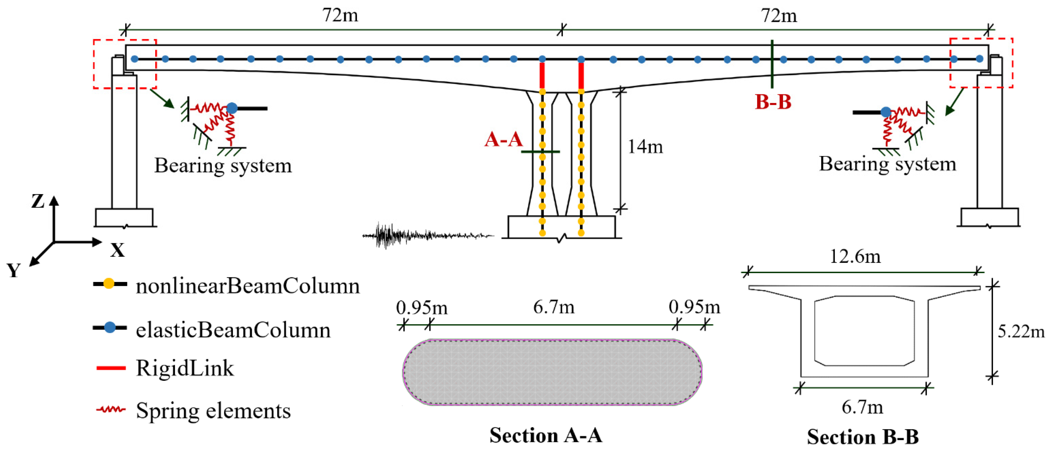
To verify the feasible and effectiveness of the proposed strategy, a (72 + 72) m high-speed railway bridge comprising a prestressed concrete continuous rigid frame under horizontal seismic loading was modeled in OpenSees [41], and the layout of the bridge model is shown in Figure 1. Based on its blueprints, the total length of the structure is 144 m, and the height of the girders varies parabolically from 5.5 m at the pier table to 2.5 m at end of the girder. The section dimensions of the bridge pier (Section A-A) and girder (Section B-B) can be found in Figure 1, respectively. Also, note that the substructure of the bridge was designed as a twin- and thin-walled pier structure, and the dimensions of the two thin-walled piers are the same.

In the nonlinear FE simulation of the bridge structure, the nonlinearBeamColumn element with a fiber section was applied to simulate the nonlinear dynamic characteristics of bridge piers, and the fiber section was defined by two types of concrete materials and a bilinear steel material. Specifically, uniaxial Kent–Scott–Park concrete material, called Concrete 01, was employed to characterize the stress–strain relationship of the cover concrete, and Concrete 02 was applied for confined concrete. For the Concrete 01 material, the values of the peak compressive strength and corresponding strain of the material model were $f_c^1=36 \mathrm{M}\mathrm{P}\mathrm{a}$ and ${\epsilon }_c^1=0.0020$, respectively. The residual crushing strength of the concrete and ultimate strain were defined as $f_{cu}^1=4.0 \mathrm{M}\mathrm{P}\mathrm{a}$ and ${\epsilon }_{cu}^1=0.005$, respectively. The Concrete 02 material was used to define the core concrete, and the values of the peak compressive strength $f_c^2$ and corresponding strain ${\epsilon }_c^2$ were same as those of Concrete 01, and the residual strength and the ultimate strain of the concrete material were defined as $f_{cu}^2=12.0 \mathrm{M}\mathrm{P}\mathrm{a}$ and ${\epsilon }_{cu}^2=0.0038$, respectively. In addition, the ratio between the unloading slope in concrete-crushing state and the initial slope was ${\xi }^2=0.1$. In addition, the tensile strength and softening stiffness parameters were assigned values of $f_t^2=2.4 \mathrm{M}\mathrm{P}\mathrm{a}$ and $E_t^2=1.0\times {10}^3 \mathrm{M}\mathrm{P}\mathrm{a}$, respectively. The fiber section consisted of 252 longitudinal steel bars with a diameter of 32 mm, and the hysteretic behaviors of the longitudinal rebars were defined by the modified Giuffre-Menegotto-Pinto steel material. Three primary parameters were assumed as follows: yield strength $f_s$ = 400 MPa, Young’s modulus $E_s$ = 2.0 × 10⁵ MPa, and strain–hardening ratio $b_s$ = 0.01. In addition, in this study, the girder is assumed to maintain linear–elastic behaviors during structural vibrations, and thus, the elasticBeamColumn element was used to define the girder. The linear elastic material model was applied for girder elements, and Young’s modulus was defined as $E_g=3.45\times {10}^4 \mathrm{M}\mathrm{p}\mathrm{a}$, referring to the design documents.

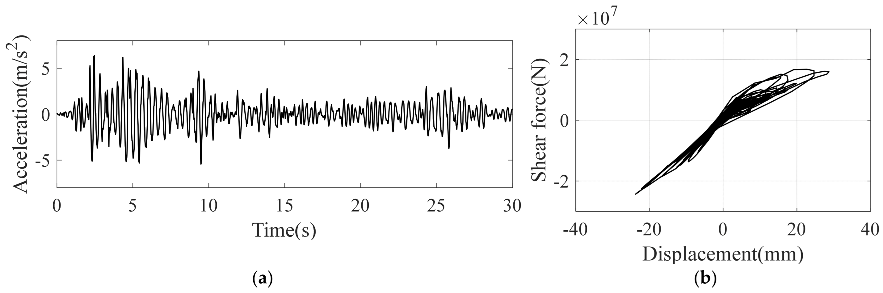
The interaction between piers and girder was modeled using the RigidLink elements, and the fixed support condition was assigned to the bottom of the bridge piers. Additionally, as observed from Figure 1, the interaction between the end-pier bearings and girder was simulated using multi-directional spring elements. Linear stiffness was assumed for spring elements in the Y- and Z-directions, and the corresponding stuffiness parameters were set as $k_y$ = 1.6 × 10⁶ N/mm and $k_z$ = 7.0 × 10⁸ N/mm, respectively. The bilinear stiffness model was employed to define nonlinear behaviors of the end-pier bearings in the X-direction, and three primary parameters were defined as follows: yield force $f_{bx}=1.2\times {10}^5 \mathrm{N}$, initial stiffness $k_x$ = 2.4 × 10⁶ N/mm, and hardening ratio $b_x=0.01$. The superstructure of the bridge is divided into 72 beam elements, and a single bridge pier consists of 12 nodes and 11 elements. The nodal mass of each element was calculated based on the product of the concrete density and corresponding volume, and the density of the concrete material was assigned a value of 24.5 kN/m³. The damping ratio of the structural system was assumed to be 0.03. To investigate the nonlinear dynamic responses of the bridge model, the regenerated ground motion record of the 1940 El Centro earthquake was employed as external excitations, and the excitation amplitude equaled 0.4 g. The Newmark-β algorithm was used to calculate structural dynamic responses with a sampling rate of 50 Hz. The obtained time history of the pier-top acceleration response is illustrated in Figure 2a, and the hysteretic curve of the base shear force and pier-top displacement is shown in Figure 2b, which shows that the bridge structure exhibits nonlinear dynamic behaviors during structural vibrations.

3.2. Probabilistic Nonlinear Model Updating of the Bridge Structure Based on VBI Approach

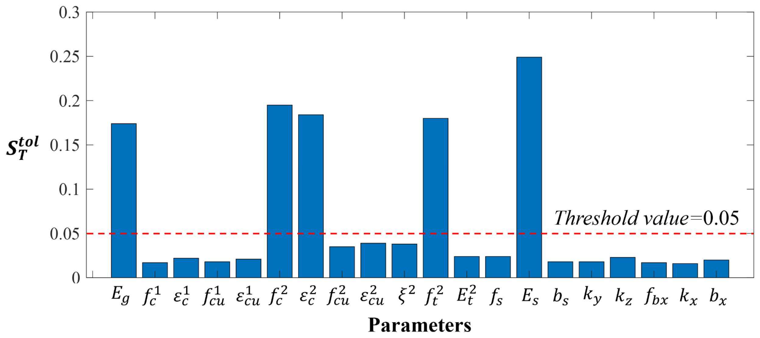
To validate the feasibility and effectiveness of the proposed method, the acceleration response measured at the pier top are considered observation data for the VBI-based probabilistic nonlinear model updating of the bridge structure. Based on the description of the bridge structure in Section 3.1, 20 model parameters, i.e., material and boundary condition parameters, may be considered possible parameters in model updating. However, selecting all parameters as candidate parameters will significantly increase the computational burden for nonlinear model updating. As a result, a variance-based global sensitivity analysis method [18] was used to rank parameters based on the calculated sensitivity indices, and high-sensitivity parameters were identified as the primary parameters for nonlinear model updating. In parameter sensitivity analysis, the feasible range of these parameters was [0.5$\mathit{\theta }$, 1.5$\mathit{\theta }$], and the calculated averaged total-order indices of 20 model parameters are illustrated in Figure 3, which can be used to quantitatively evaluate the influence of these model parameters. As observed from Figure 3, the calculated sensitivity indices of five model parameters—$E_g$, $f_c^2$, ${\epsilon }_c^2$, $f_t^2$ and $E_s$—are larger than 0.05. Thus, in this simulation, these five parameters were selected as candidate parameters for model updating when a threshold value of 0.05 was adopted.

To simulate parameter uncertainty, 50 sets of parameter vectors were randomly generated within the interval of [0.95$\mathit{\theta }$, 1.05$\mathit{\theta }$], and then, the corresponding acceleration responses of the bridge structure were obtained via nonlinear dynamic analysis. Since the amplitudes of acceleration responses slowly vary with time compared with the oscillation of the time histories, it is not necessary to select all measured data points as the input for the proposed nonlinear model updating approach. However, if too few data are selected, the selected time series may lose the original statistical characteristics. Therefore, in this study, to improve the computational efficiency of the VBI-based model updating approach, 10% of data points uniformly selected from the instantaneous amplitudes of the measured acceleration responses were used as the measured data, and the feasibility of this downsampling method has been verified in previous studies [9,42].

Prior to nonlinear model updating, surrogate model techniques were employed to characterize the relationship between model parameters and observation data, which aims to replace computationally expensive high-fidelity FE simulations. Therefore, to train a GP surrogate model, 500 sets of candidate parameter vectors were generated using the Latin Hypercube Sampling method [43,44], and the corresponding data samples were obtained via nonlinear FE analysis. After the GP model was well trained, it was used for structural responses prediction in VBI-based nonlinear model updating.

3.2.1. Nonlinear Model Updating Subjected to Measurement Noises

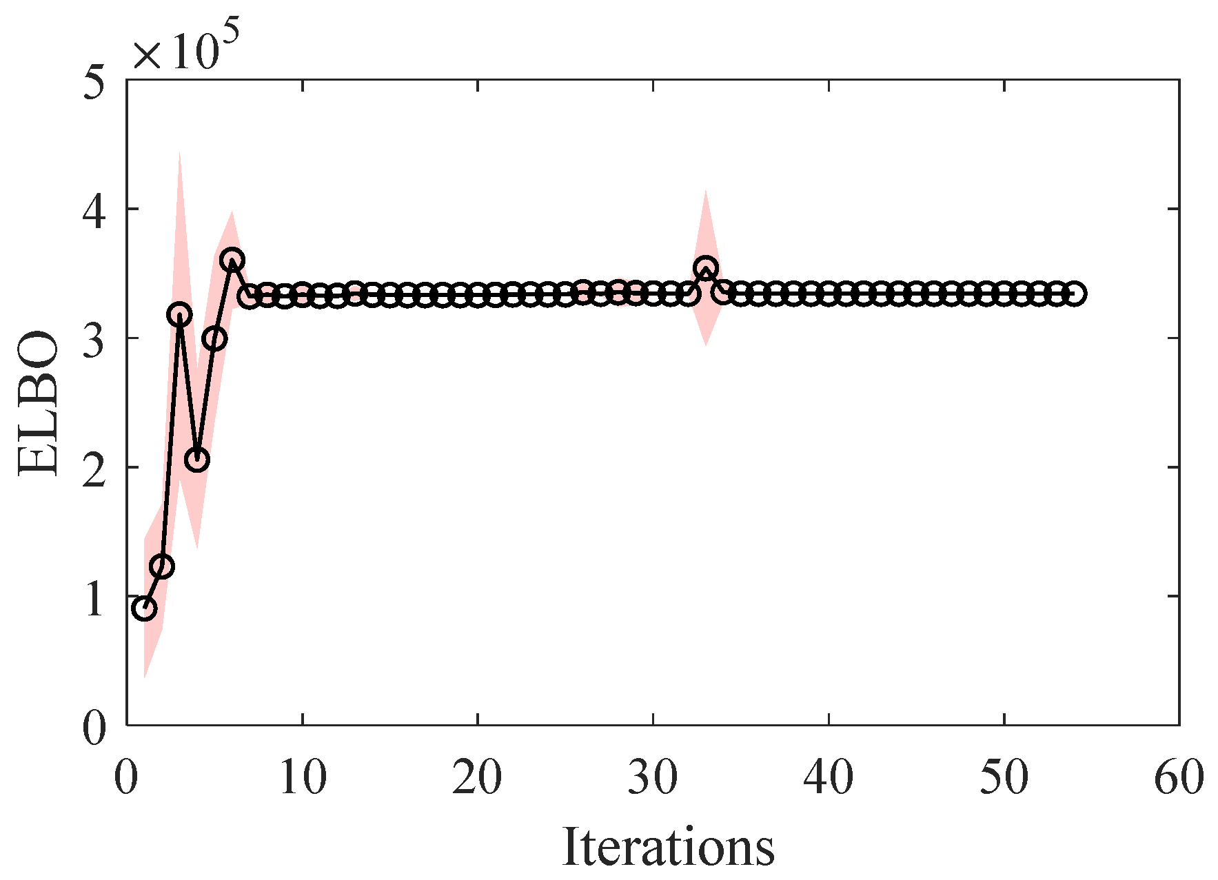
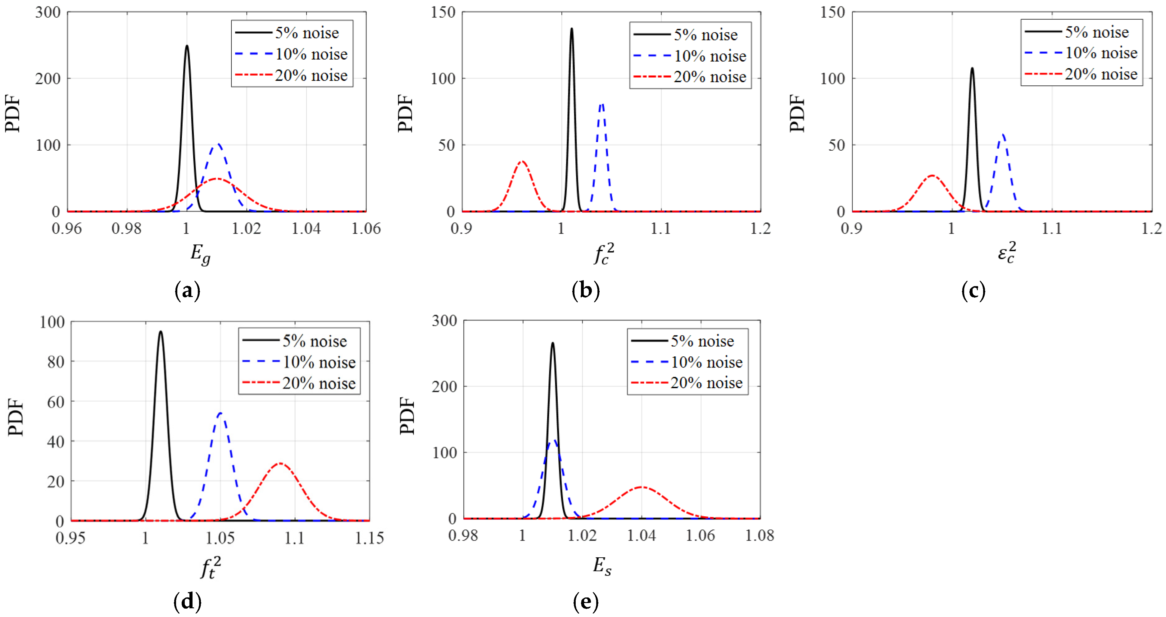
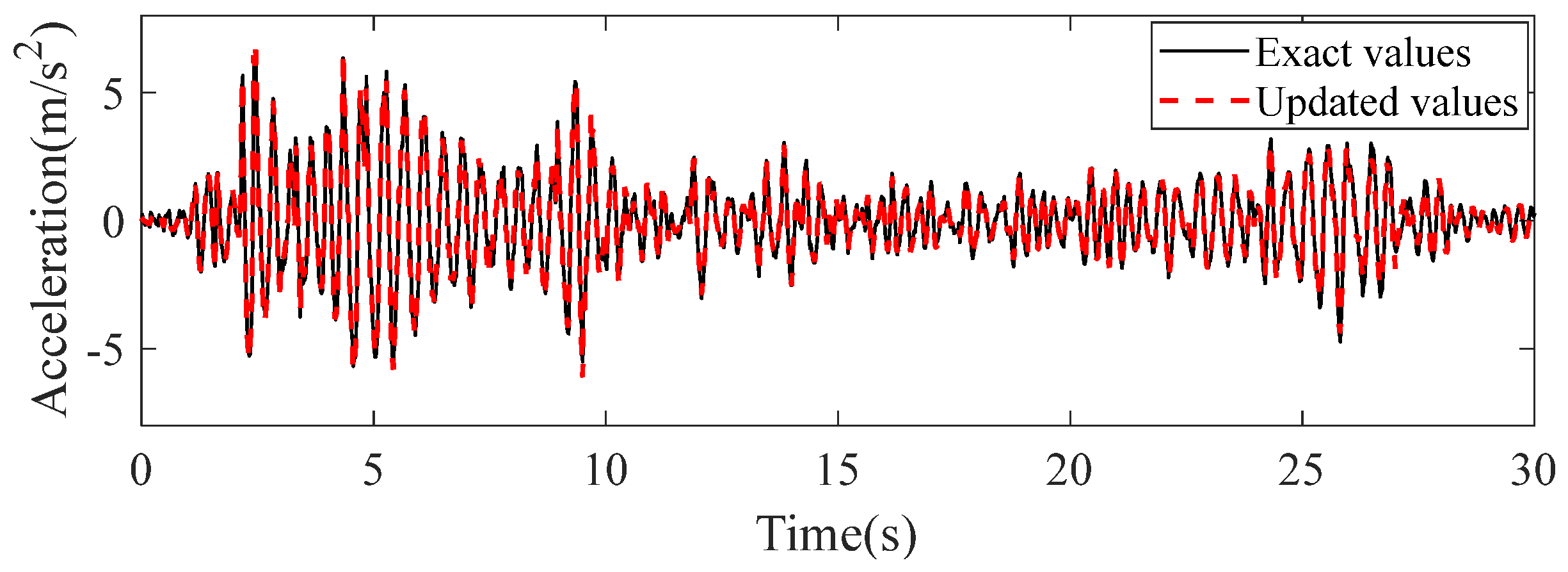
Since structural dynamic responses are inevitably contaminated by measurement noise during data collection and transmission, in this simulation, nonlinear model updating was investigated under 5%, 10%, and 20% measurement noise. During nonlinear model updating, the prior distributions of five model parameters were assumed to follow a Gaussian distribution, and the initial values of these parameters were set as follows: $E_g~N\left(0.75,0.2\right),$ $f_c^2~N\left(0.85, 0.2\right),$ ${\epsilon }_c^2~N\left(1.05, 0.2\right),$ $f_t^2~N\left(0.85, 0.2\right),$ and $E_s~N\left(1.15,0.2\right)$. Subsequently, variational inference was performed for the posterior distribution estimation of five model parameters. The initial number of Gaussian components was assumed to be 2, and the corresponding weight coefficients were 0.5. The surrogate model of $g\left(\mathit{\theta }\right)$ was first trained with 50 training samples, and 5 additional best samples were added to the training set in each subsequent iteration. The computing device used for this simulation was a desktop computer with an Intel(R) Core (TM) i7-10700 (2.90 GHz) processor and 16 GB of RAM, and the runtimes of three cases were 65.14 s, 55.44 s, and 37.32 s. The hyperparameters were optimized for these three cases by performing the proposed procedure described in Table 1. The convergence curve of the ELBO under 5% measurement noise is shown in Figure 4; note that the fluctuation in the ELBO is relatively large before the first six iterations, and then, the fluctuation becomes considerably small after the 35th iteration. The value of the ELBO finally converges to 3.343 × 10⁵ when the number of iterations reaches 54. After the iteration process terminates, the effective numbers of Gaussian components for these cases are 5, 5, and 6, respectively, and the minimum value of the weights is larger than 0.1. The approximate posterior PDFs of five model parameters can be found in Figure 5, and the detailed calibrated results are presented in

Table 2. Calibrated results of model parameters under measurement noise effects.

Para.	${\mathit{E}}_{\mathit{g}}$		${\mathit{f}}_{\mathit{c}}^{\mathbf{2}}$		${\mathit{\epsilon }}_{\mathit{c}}^{\mathbf{2}}$		${\mathit{f}}_{\mathit{t}}^{\mathbf{2}}$		${\mathit{E}}_{\mathit{s}}$
	Mean Value	C.O.V (%)	Mean Value	C.O.V (%)	Mean Value	C.O.V (%)	Mean Value	C.O.V (%)	Mean Value	C.O.V (%)
5%	1.00	0.16	1.01	0.29	1.02	0.37	1.01	0.42	1.01	0.15
10%	1.01	0.39	1.04	0.48	1.05	0.69	1.05	0.74	1.01	0.33
20%	1.01	0.81	0.96	1.06	0.98	1.48	1.09	1.39	1.04	0.84

. Additionally, the predicted acceleration responses of the bridge structure based on the calibrated nonlinear FE model is shown in Figure 6. Compared to the measured acceleration responses, these results indicate that the updated model can accurately predict nonlinear dynamic responses of the structure subjected to earthquake excitations. The relative squared error of the instantaneous amplitudes of the measured and updated acceleration responses is 4.35%. In addition, Table 2 shows that the five model parameters can be accurately calibrated based on the proposed approach, and the maximum error of the calibrated parameters is below 10% even under 20% measurement noise. In addition, note that the estimated coefficient of variation (C.O.V) of the five model parameters gradually increases with the increased noise level, and the maximum C.O.V of parameter ${\epsilon }_c^2$ reaches 1.48%. The results indicate that the proposed method is accurate and reliable for probabilistic nonlinear model updating with improved noise robustness.

To verify the effectiveness and advantages of the proposed VBI-based nonlinear model updating strategy, comparative analysis with the conventional Bayesian approach [16] was conducted in this study. In Bayesian-based nonlinear model updating, the same measured data and initial parameters were applied, and the Metropolis–Hastings (MH) stochastic sampling algorithm was employed for the posterior distribution estimation of model parameters, during which the maximum number of iterations and sampling acceptance rate of the MH algorithm were set to 20,000 and 0.1, respectively. The required runtime was 154.88 s. In contrast, when variational inference was employed for nonlinear model updating, the required runtime was only 65.14 s, which is considerably lower than that of conventional Bayesian methods.

Table 3. Comparison of calibrated results based on two different methods.

Para.	${\mathit{E}}_{\mathit{g}}$		${\mathit{f}}_{\mathit{c}}^{\mathbf{2}}$		${\mathit{\epsilon }}_{\mathit{c}}^{\mathbf{2}}$		${\mathit{f}}_{\mathit{t}}^{\mathbf{2}}$		${\mathit{E}}_{\mathit{s}}$
	Mean Value	C.O.V (%)	Mean Value	C.O.V (%)	Mean Value	C.O.V (%)	Mean Value	C.O.V (%)	Mean Value	C.O.V (%)
VBI	1.00	0.16	1.01	0.29	1.02	0.37	1.01	0.42	1.01	0.15
MH	0.98	0.31	1.01	0.48	1.04	0.63	0.95	0.71	1.00	0.49

presents the statistical results for five candidate parameters after removing 1200 burn-in samples. Note that the calibration error for the model parameters reaches 5%, and the estimated uncertainties of these parameters are also larger than those for the proposed approach. This phenomenon is primarily attributed to the randomness of the structural parameters, which may cause non-Gaussian posterior distributions for the model parameters. As a result, the estimated nonlinear parameters may deviate from their real values. In contrast, given the advantages of GMMs in approximating probability distributions, a GMM is an effective means for probabilistic nonlinear model updating with hyperparameter optimization.

3.2.2. Nonlinear Model Updating Subjected to Modeling Errors

In the FE modeling of complex engineering structures, model simplification techniques are often applied to improve computational efficiency; however, this inevitably causes a series of modeling errors between FE models and real structures. To investigate the effects of modeling errors on the accuracy of nonlinear model updating, two types of modeling errors—nodal mass and damping ratios—are considered, and two error levels (5% and 10%) are further studied via simulation. In total, four different modeling errors were studied: 5% mass error, 10% mass error, 5% damping ratio error, and 10% damping error. Based on the initial nonlinear model described in Section 3.2.1 and VBI approach, the calibration results of the model parameters are listed in

Table 4. The calibrated nonlinear parameters subjected to various modeling errors.

Para.	${\mathit{E}}_{\mathit{g}}$		${\mathit{f}}_{\mathit{c}}^{\mathbf{2}}$		${\mathit{\epsilon }}_{\mathit{c}}^{\mathbf{2}}$		${\mathit{f}}_{\mathit{t}}^{\mathbf{2}}$		${\mathit{E}}_{\mathit{s}}$
	Mean Value	C.O.V (%)	Mean Value	C.O.V (%)	Mean Value	C.O.V (%)	Mean Value	C.O.V (%)	Mean Value	C.O.V (%)
Case 1	0.99	0.36	1.02	0.39	1.04	0.67	1.00	0.56	1.02	0.31
Case 2	1.06	0.79	0.98	0.82	1.11	1.58	0.94	1.02	1.06	0.68
Case 3	1.01	0.20	1.00	0.28	1.03	0.43	1.01	0.29	0.98	0.31
Case 4	0.98	0.41	1.03	0.41	1.05	0.89	1.00	0.52	0.96	0.54

, which shows that the model parameters of the four cases are close to their real values and the parameter uncertainty level is significantly increased at increased error levels. Moreover, note that the effects of mass error are larger than those of the damping ratio, and the maximum calibration error of the model parameters reaches 11.0% when subjected to 10% mass error. This analysis reveals that modeling errors significantly affect the calibration results of model parameters. Thus, it is necessary to further investigate the effects of other types of modeling errors, i.e., boundary conditions, material constitutive models, etc., in nonlinear model updating, especially for complex engineering structures.

3.3. Failure Probability Estimation of the Bridge Structure Based on the SS Algorithm

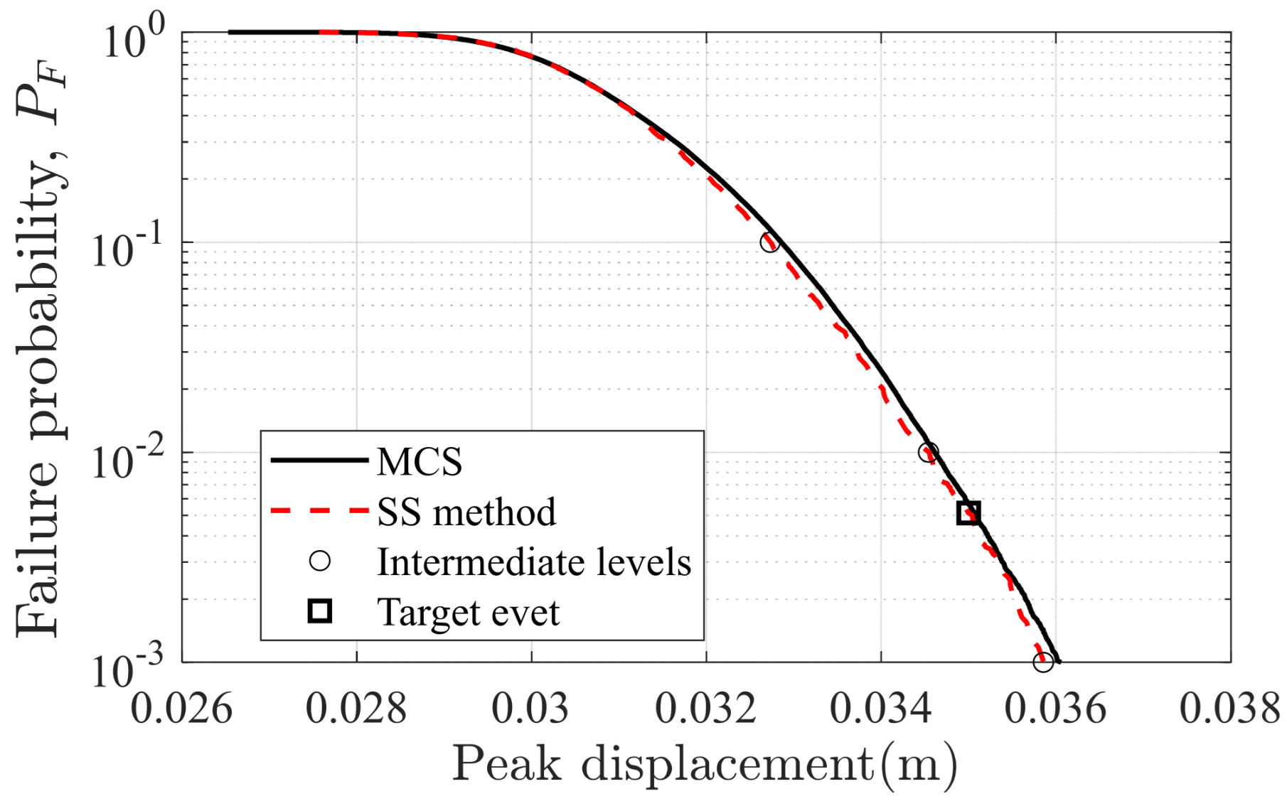
The primary purpose of structural reliability evaluation is to quantitatively evaluate the safety performance of structures from a probabilistic perspective. Based on the calibrated nonlinear structural model described in Section 3.2.1, the failure probability of the bridge structure subjected to three different types of strong seismic excitations were investigated using the SS algorithm. Simultaneously, to consider the effects of the excitation types, three regenerated typical seismic records, shown in

Table 5. The applied external excitations.

No	Event	Station	Year	Original PGA (g)	Regenerated PGA (g)	Amplitude Uncertainty
1	Imperial Valley	Niland Fire	1979	0.108	0.4	10%
2	Imperial Valley	Chihuahua	1979	0.270	0.5	10%
3	Northridge	Newhall Fire	1994	0.566	0.6	10%

, were selected as external excitation sources for the bridge structure, and the randomness of the applied excitation amplitudes were also considered in this study. In the structural failure probability calculation, the peak displacement at the pier top is defined as a safety index, and then, the SS algorithm with parameters $p_0=0.1$ and $N_i=1000$ was used to compute the failure probability of the bridge structure subjected to strong ground motions. In the numerical simulation, the failure event was defined using the maximum longitudinal displacements of the pier subjected to seismic excitations, denoted as $u_{max}\left(t\right)$. When $u_{max}\left(t\right)$ exceeds the response threshold of 0.035 m, a failure event occurs. Using the SS algorithm, the obtain failure probability curve of the bridge structure subjected to regenerated seismic loading with PGA of 0.4 g was obtained, as shown in Figure 7, where it can be seen that three subset regions were adaptively constructed in the computational process, with threshold values of 0.0327, 0.0345, and 0.0359, respectively. The calculated failure probability of the structure is 5.14 × 10⁻³, and the computation time for this event is about 7.63 h, using an interactive computational strategy coupling MATLAB (v R2022b) and OpenSees (v3.0.0a) for the computation. Additionally, to verify the accuracy of the calculation results, the MCS method was then used to estimate the failure probability of the structure. Based on the calibrated model, a total of 1 × 10⁵ MCS iterations were performed to estimate the structural failure probability, and about 112.38 h were required to complete this simulation. The generated failure probability curve of the MCS method is shown in Figure 7. Compared with the failure probability estimation results presented in Figure 7, the failure probability curves estimated from these two approaches are substantially consistent. However, the computational cost of the MCS method is considerably higher than that of the SS algorithm. Therefore, the results indicate that the SS method can provide accurate failure probability estimation for structures with low computing cost. Subsequently, based on the SS approach, the calculated failure probabilities of three events are 5.14 × 10⁻³, 0.135, and 0.488, respectively, which slightly increase with an increased PGA of the applied seismic excitations; when the PGA reaches 0.6 g, the estimated failure probability of the bridge structure is 0.488, which indicates that severe structural damage may occur when subjected to such seismic excitation. Therefore, based on this analysis, the proposed approach is reliable and effective for the reliability assessment of nonlinear structures subjected to seismic loads.

Additionally, to further investigate the uncertainty propagation from posterior parameters to failure probability, the updated nonlinear models presented in Table 2 were used for structural failure probability calculations. In this simulation, the second seismic load described in Table 5 was selected as the external excitation for the three nonlinear models. Based on the updated nonlinear models and SS algorithm, the failure probability of the bridge structure was calculated using an interactive computational strategy coupling MATLAB and OpenSees. The calculated failure probabilities of the bridge structure are 0.135, 0.159, and 0.263, respectively, and the results indicate that the posterior uncertainty of the model parameters has a significant influence on the structural failure probability calculation, and the maximum variation reaches 94.8%. Thus, it is necessary to accurately quantify posterior distributions of model parameters before assessing structural reliability.

4. Experimental Verification

4.1. Shaking Table Test Structure

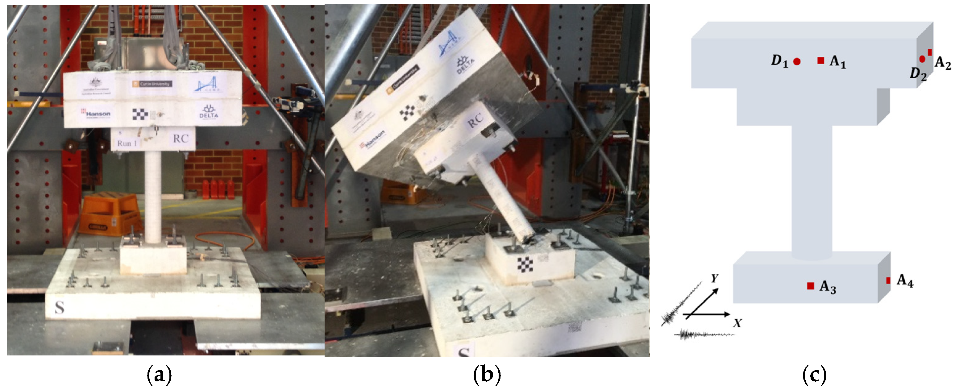
A 1/12 scaled reinforced concrete (RC) column shake table structure was experimentally investigated, and the tested structure is shown in Figure 8a. The total length of the tested structure was 0.9 m, including a (400 mm × 400 mm × 150 mm) footing and (500 mm × 500 mm × 150 mm) cap, respectively, and the cross-section diameter of the column structure was 0.1 m. Based on the material testing report, the compressive strength of the applied concrete material was 37.0 MPa, and the ultimate strengths of the longitudinal rebars and stirrups were 616 MPa and 430 MPa, respectively. The detailed geometric and material parameters of the tested structure can be found in the literature [45]. To record structural dynamic responses subjected to external excitations, six sensors, including four accelerometers (A₁–A₄) and two laser displacement sensors (D₁ and D₂), were installed on the structure, and the layout of these sensors can be seen in Figure 8c. The sampling rate of all sensors was set to 200 Hz. The applied excitation of the tested structure was regenerated based on the 1979 Imperial Valley earthquake records. The peak ground accelerations (PGA) in two directions were 0.108 g and 0.068 g, respectively. The regenerated seismic loads in two directions were scaled by referring to the maximum PGA value in the X-direction, increasing from 0.2 g with an interval of 0.1 g up to column collapse, and the ratio of PGA in two directions remained unchanged. Based on previous studies [46,47], the RC column was finally destroyed when the applied excitation amplitude in the X-direction reached 0.1 g, and the collapsed structure is shown in Figure 8b. In this study, the measured structural responses subjected to seismic load with PGA of 0.5 g were employed for the nonlinear model updating of the tested structure.

4.2. Nonlinear Model Updating of RC Column Structure Based on VBI Approach

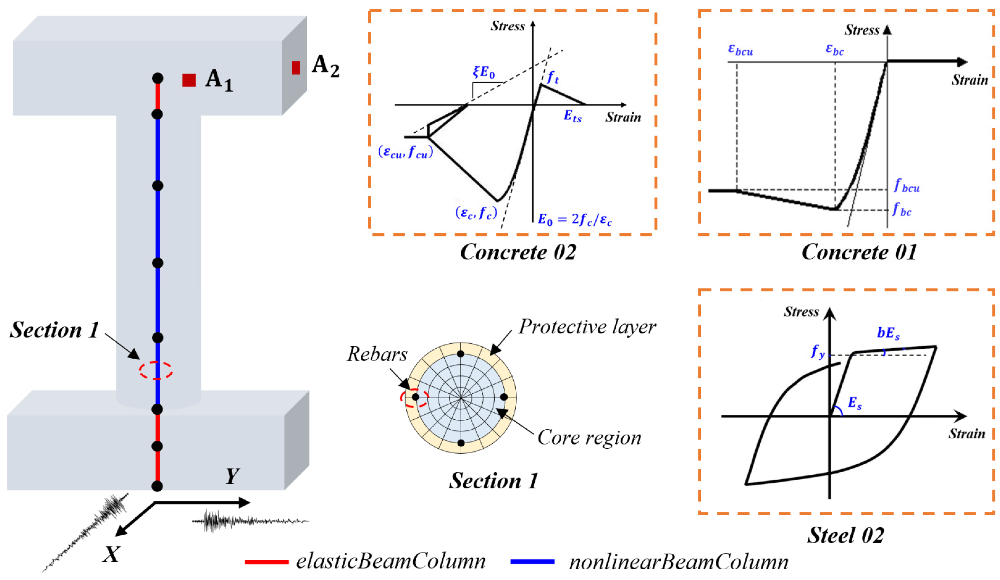
Based on the design documents and material testing reports, an initial nonlinear FE model was built in OpenSees, as illustrated in Figure 9. In this FE model, the RC column is defined by force-based beam-column elements with a fiber section that consists of three parts: a protective layer, a core region, and rebars. The Kent–Park constitutive model, called Concrete 01, was used for the protective layer of the fiber section, and four primary material parameters were assigned as follows: $f_c^1=37.0 \mathrm{M}\mathrm{P}\mathrm{a}$, the strain at the peak compressive strength ${\epsilon }_c^1=0.0025$, and the final crushing strength of concrete and corresponding crushing strength $f_{cu}^1=5.0 \mathrm{M}\mathrm{P}\mathrm{a}$ and ${\epsilon }_{cu}^1=0.01$, respectively. Additionally, the Concrete02 constitutive model was employed as the concrete material in the core region, and the peak compressive strength was set to $f_c^1=37.0 \mathrm{M}\mathrm{P}\mathrm{a}$, with the strain at the peak compressive strength defined as ${\epsilon }_c^1=0.0025$, the final crushing strength of the concrete and corresponding crushing strength defined as $f_{cu}^1=12.0 \mathrm{M}\mathrm{P}\mathrm{a}$ and ${\epsilon }_{cu}^1=0.0038$, respectively, and the ratio between the unloading slope at the concrete-crushing state and the initial slope defined as $\xi =0.1$. In addition, the tensile strength and softening stiffness parameters were set as $f_t=2.0 \mathrm{M}\mathrm{P}\mathrm{a}$ and $E_{ts}=1.0\times {10}^3 \mathrm{M}\mathrm{P}\mathrm{a}$, respectively. Moreover, modified Giuffre-Menegotto-Pinto steel material was used to define the hysteretic characteristics of steel rebars. Three primary parameters are set as follows: yield strength $f_s=555 \mathrm{M}\mathrm{P}\mathrm{a}$, Young’s modulus $E_s=2.0\times {10}^5 \mathrm{M}\mathrm{P}\mathrm{a}$, and strain-hardening ratio $b_s=0.05$. The constitutive relationships of the three materials are shown in Figure 9. Subsequently, the footing and cap components were simulated as linear–elastic elements, with a Young’s modulus of $3.0\times {10}^4 \mathrm{M}\mathrm{P}\mathrm{a}$. For the above-mentioned material parameters, since the compressive strength of the concrete material and the tensile strength of the steel material was tested before shake table testing, these parameters were considered to be accurate. Therefore, based on parameter sensitivity analysis, six material parameters were finally selected to represent the nonlinear dynamic characteristics of the tested structure subjected to seismic excitations, denoted as $\mathit{\theta }=\left\{{\epsilon }_c^1,f_{cu}^1,{\epsilon }_{cu}^1,{\epsilon }_c^2,E_s,b_s\right\}$. The damping ratio of the nonlinear model was set to 0.04, and the acceleration responses recorded from Accelerometers A₃ and A₄ were set as external loads of the structure.

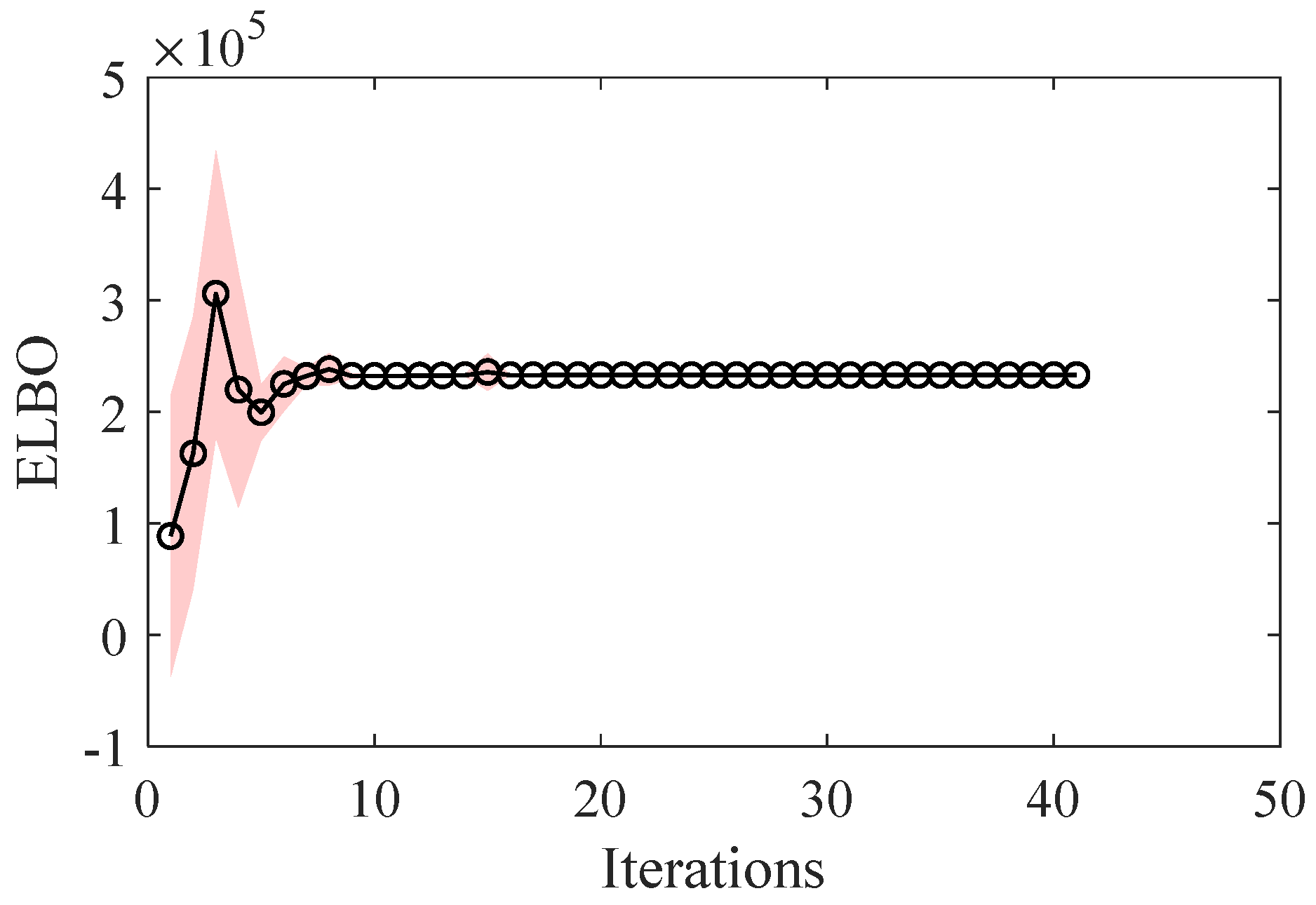
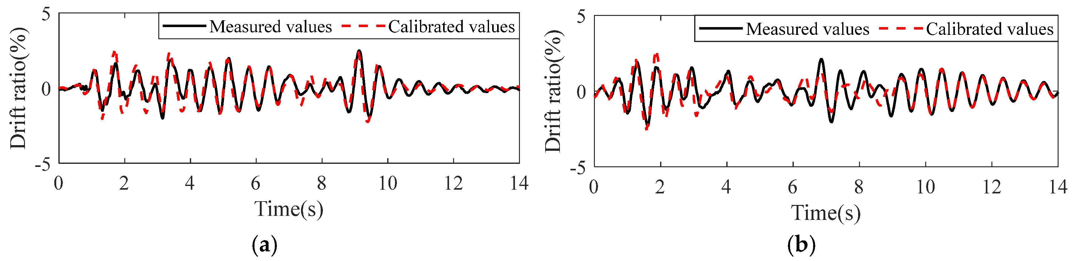
In the nonlinear model updating of the tested structure, due to a lack of sufficient vibration test data, 50 sets of acceleration response samples of the tested structure were generated by introducing a scale factor into the measured structural responses, and these obtained datasets were used to calibrate the model of the column structure. Then, according to the VBI-based model updating procedure, the prior distribution of six model parameters was assumed to follow a Gaussian distribution, the designated values of these parameters were assigned as their mean values, and the prior variances for all parameters were set to $0.2{\mathit{\theta }}^{\mathbf{0}}$ (where ${\mathit{\theta }}^{\mathbf{0}}$ denotes the set values of the model parameters). Subsequently, the VBI method was used for the posterior PDF estimation of the six model parameters, and the convergence curve of the ELBO is presented in Figure 10. Note that the convergence curve of the ELBO shows a significant fluctuation trend in the first nine iterations, and then, the uncertainty level of the calculated ELBO is significantly small. The optimization process terminates after performing 40 iterations, and the corresponding value of the ELBO is 2.330 × 10⁵. When the convergence criteria are satisfied, the effective number of Gaussian components is 8, and the minimum value of the weights is larger than 0.1. The statistical results of the posterior PDFs for six model parameters are summarized in

Table 6. The calibrated model parameters of the tested structure.

Para.	${\mathit{\epsilon }}_{\mathit{c}}^{\mathbf{1}}/{\left\{{\mathit{\epsilon }}_{\mathit{c}}^{\mathbf{1}}\right\}}^{\mathbf{0}}$	${\mathit{f}}_{\mathit{c}\mathit{u}}^{\mathbf{1}}/{\left\{{\mathit{f}}_{\mathit{c}\mathit{u}}^{\mathbf{1}}\right\}}^{\mathbf{0}}$	${\mathit{\epsilon }}_{\mathit{c}\mathit{u}}^{\mathbf{1}}/{\left\{{\mathit{\epsilon }}_{\mathit{c}\mathit{u}}^{\mathbf{1}}\right\}}^{\mathbf{0}}$	${\mathit{\epsilon }}_{\mathit{c}}^{\mathbf{2}}/{\left\{{\mathit{\epsilon }}_{\mathit{c}}^{\mathbf{2}}\right\}}^{\mathbf{0}}$	${\mathit{E}}_{\mathit{s}}/{\left\{{\mathit{E}}_{\mathit{s}}\right\}}^{\mathbf{0}}$	${\mathit{b}}_{\mathit{s}}/{\left\{{\mathit{b}}_{\mathit{s}}\right\}}^{\mathbf{0}}$
Mean value	0.93	1.13	0.95	1.08	0.95	1.16
C.O.V (%)	2.15	4.11	3.53	3.24	2.67	4.55

. In addition, the calibrated structural displacement responses in the X- and Y-directions can be found in Figure 11, which also shows that the calibrated nonlinear model can accurately predict structural displacement responses, resulting in substantial improvement in the accuracy and robustness of the structural reliability evaluation.

4.3. Failure Probability Estimation of the RC Column Structure

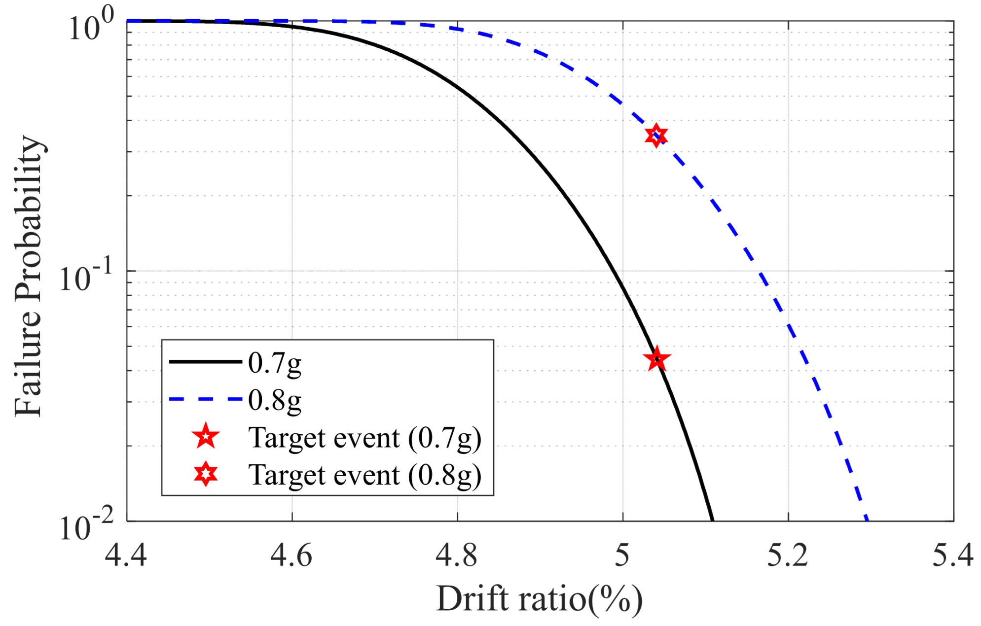
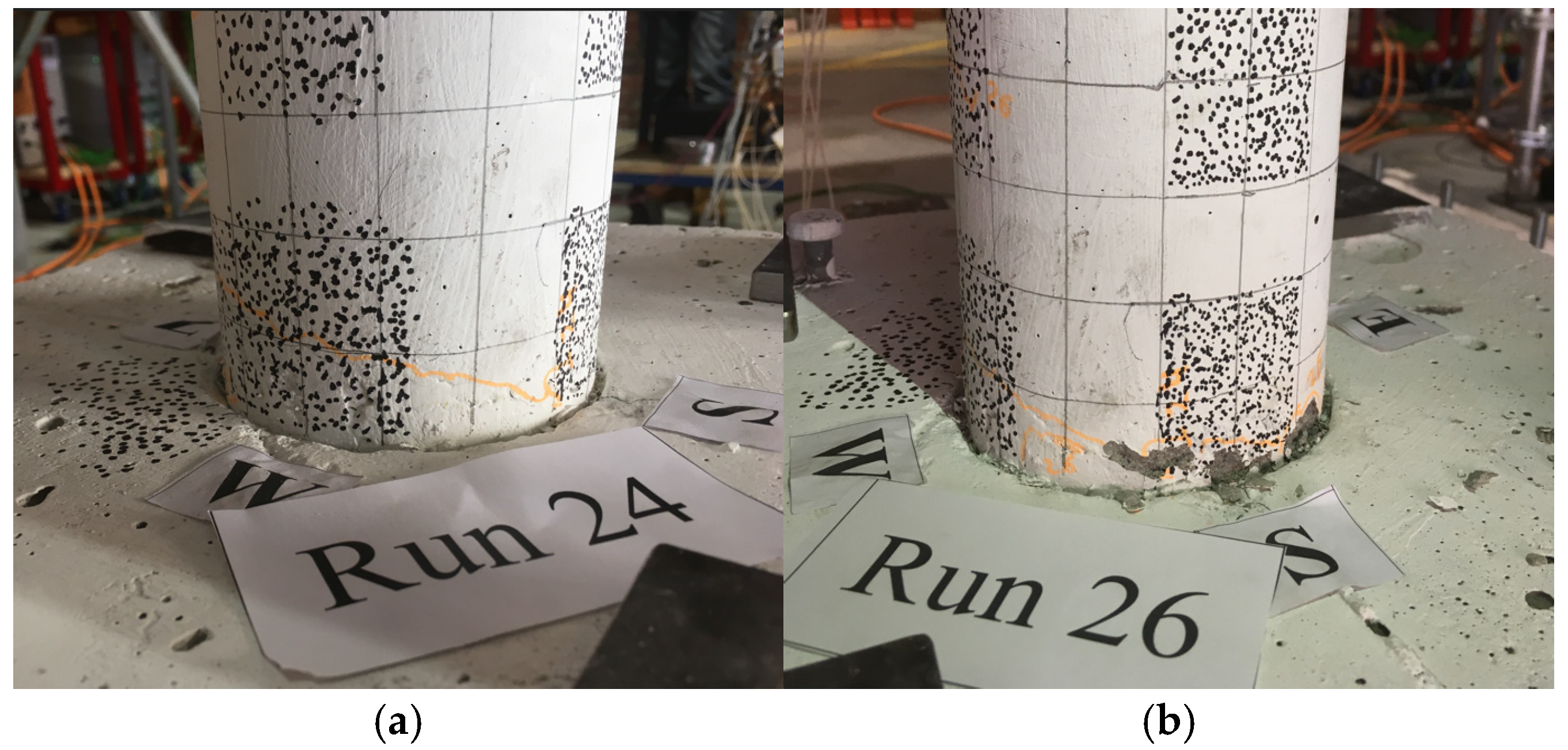
After the nonlinear model of the tested structure is updated, it can be used to estimate the failure probability of the column structure subjected to seismic excitations with an amplitude of 0.7 g or 0.8 g. Referring to the experimental description in Section 4.1, since the applied excitation amplitude in the X-direction of the tested structure is larger than that in the structural Y-direction, only the failure probability of the tested structure in the X-direction was investigated in this study. Similarly to in the numerical simulation, the SS algorithm with parameters $p_0=0.1$ and $N_i=1000$ was used to compute the failure probability of the column structure subjected to strong ground motions. In the experiment, the failure event is defined using the maximum drift ratio of the column structure subjected to seismic excitations, denoted as $D_{max}\left(t\right)$. When $u_{max}\left(t\right)$ exceeds the response threshold of 5.04%, the failure event occurs. Based on the results of the SS algorithm, the estimated failure probability curves of the column structure subjected to seismic loadings with PGA of 0.7 g and 0.8 g are presented in Figure 12, which also shows that the estimated failure probabilities of the structure are 0.042 and 0.348, respectively. This phenomenon indicates that structural damage gradually increases with an increasing excitation amplitude, and severe damage may occur after a 0.8 g earthquake load is applied. Based on the shake table testing results, the actual damage state of the column structure subjected to these two types of seismic excitations is presented in Figure 13. Figure 13a features a long crack along the bottom of the tested structure, which indicates that moderate damage occurred after 0.7 g seismic excitation was applied. In addition, as can be seen in Figure 13b, the concrete at the bottom of the column was partially crushed when the applied excitation amplitude reached 0.8 g, meaning that the cumulative damage of the tested structure was severe after 0.8 g seismic excitation was applied. Therefore, based on the above analysis, the predicted failure probability is reasonable for interpreting the damage conditions of a tested structure subjected to strong seismic loads. Meanwhile, the investigation results validate the effectiveness and accuracy of the proposed reliability assessment procedure.

5. Conclusions

In this study, variational inference with GMMs was applied for probabilistic nonlinear model updating based on measured structural responses. Then, the calibrated nonlinear model was employed to enhance the reliability evaluation of structures subjected to strong seismic excitations. The following conclusions can be drawn from numerical simulations and experimental verifications:

(1) Variational inference with GMMs is effective and reliable for the probabilistic model updating of nonlinear structures, even under significantly noisy measurement conditions. In particular, when 20% Gaussian white noise is added to structural responses, the proposed method still achieves a parameter estimation error of less than 10%. This demonstrates its strong robustness against measurement noise.

(2) Using stochastic gradient descent and active learning strategies, the optimal hyperparameters of the GMMs can be obtained by maximizing the ELBO, and the optimized GMMs can be used to effectively approximate the posterior PDFs of nonlinear model parameters.

(3) Based on the calibrated posterior PDFs of nonlinear model parameters, the accuracy and robustness of the structural reliability evaluation substantially improved. Specifically, for the scaled column structure subjected to strong seismic excitations with a PGA of 0.7 or 0.8 g, the estimated failure probabilities obtained using the calibrated model were more reasonable for the interpretation of the damage conditions of the tested structure.

(4) Although variational inference with GMMs provides a promising framework for the probabilistic nonlinear model updating of structures, the number of hyperparameters becomes prohibitively large when applying the proposed method to high-dimensional parameter spaces. Therefore, achieving a balance between computational efficiency and posterior approximation accuracy for nonlinear model parameters remains an issue that requires further investigation.

References

1. Hao, H.; Bi, K.; Chen, W.; Pham, T.M.; Li, J. Towards next generation design of sustainable, durable, multi-hazard resistant, resilient, and smart civil engineering structures. Eng. Struct. 2023, 277, 115477. [Google Scholar] [CrossRef]
2. Simoncelli, M.; Aloisio, A.; Zucca, M.; Venturi, G.; Alaggio, R. Intensity and location of corrosion on the reliability of a steel bridge. J. Constr. Steel Res. 2023, 206, 107937. [Google Scholar] [CrossRef]
3. Dong, C.-Z.; Catbas, F.N. A review of computer vision–based structural health monitoring at local and global levels. Struct. Health Monit. 2021, 20, 692–743. [Google Scholar] [CrossRef]
4. Huang, J.; Broekman, A.; Markou, G.; Chen, H.-P. Framework for a practical and cost-effective IoT-enhanced structural health monitoring and damage diagnostics system with digital twinning. J. Civ. Struct. Health Monit. 2025, 15, 2059–2084. [Google Scholar] [CrossRef]
5. Wu, S.; Liu, J. A Multi-Scale CNN-BiLSTM Framework with an Attention Mechanism for Interpretable Structural Damage Detection. Infrastructures 2025, 10, 82. [Google Scholar] [CrossRef]
6. Chen, B.; Starman, B.; Halilovič, M.; Berglund, L.A.; Coppieters, S. Finite Element Model Updating for Material Model Calibration: A Review and Guide to Practice. Arch. Comput. Methods Eng. 2024, 32, 2035–2112. [Google Scholar] [CrossRef]
7. Xin, Y.; Li, J.; Wang, X.; Hampson, K. Load-carrying capacity assessment of an existing highway bridge based on hybrid finite-element model updating. J. Perform. Constr. Facil. 2022, 36, 04022028. [Google Scholar] [CrossRef]
8. Tamuly, P.; Chakraborty, A.; Das, S. Nonlinear finite element model updating using constrained unscented Kalman filter for condition assessment of reinforced concrete structures. J. Civ. Struct. Health Monit. 2021, 11, 1137–1154. [Google Scholar] [CrossRef]
9. Xin, Y.; Hao, H.; Li, J.; Wang, Z.C.; Wan, H.P.; Ren, W.X. Bayesian based nonlinear model updating using instantaneous characteristics of structural dynamic responses. Eng. Struct. 2019, 183, 459–474. [Google Scholar] [CrossRef]
10. Pan, J.; Chen, X.; Mu, D.; Zeng, Y.; Guan, Z. An analytical sensitivity-based model updating for nonlinear systems using Nonlinear Normal Modes. Mech. Syst. Signal Process. 2025, 231, 112628. [Google Scholar] [CrossRef]
11. Ebrahimian, H.; Astroza, R.; Conte, J.P.; de Callafon, R.A. Nonlinear finite element model updating for damage identification of civil structures using batch Bayesian estimation. Mech. Syst. Signal Process. 2017, 84, 194–222. [Google Scholar] [CrossRef]
12. Ding, Y.J.; Wang, Z.C.; Chen, G.D.; Ren, W.X.; Xin, Y. Markov Chain Monte Carlo-based Bayesian method for nonlinear stochastic model updating. J. Sound Vib. 2022, 520, 116595. [Google Scholar] [CrossRef]
13. Jang, J.; Smyth, A. Bayesian model updating of a full-scale finite element model with sensitivity-based clustering. Struct. Control Health Monit. 2017, 24, E2004. [Google Scholar] [CrossRef]
14. Nabiyan, M.-S.; Ebrahimian, H.; Moaveni, B.; Papadimitriou, C. Adaptive Bayesian inference framework for joint model and noise identification. J. Eng. Mech. 2022, 148, 04021165. [Google Scholar] [CrossRef]
15. Yuan, Z.-Q.; Kuang, X.-C.; Wang, Z.-C.; Xin, Y.; Jiang, Y.-P. A probabilistic method for structural model updating using a model-data hybrid driven technique. Structures 2025, 77, 109057. [Google Scholar] [CrossRef]
16. Ding, Y.-J.; Wang, Z.-C.; Xin, Y. Gaussian process metamodel and Markov chain Monte Carlo-based Bayesian inference framework for stochastic nonlinear model updating with uncertainties. Probabilistic Eng. Mech. 2023, 75, 103576. [Google Scholar] [CrossRef]
17. Pandey, P.; Khodaparast, H.H.; Friswell, M.I.; Chatterjee, T.; Madinei, H.; Deighan, T. Stochastic nonlinear model updating in structural dynamics using a novel likelihood function within the Bayesian-MCMC framework. Appl. Math. Model. 2024, 138, 115800. [Google Scholar] [CrossRef]
18. Ramancha, M.K.; Astroza, R.; Madarshahian, R.; Conte, J.P. Bayesian updating and identifiability assessment of nonlinear finite element models. Mech. Syst. Signal Process. 2022, 167, 108517. [Google Scholar] [CrossRef]
19. Jia, X.; Sedehi, O.; Papadimitriou, C.; Katafygiotis, L.S.; Moaveni, B. Nonlinear model updating through hierarchical Bayesian modeling framework. Comput. Methods Appl. Mech. Eng. 2022, 392, 114646. [Google Scholar] [CrossRef]
20. Wan, H.-P.; Ren, W.-X. Stochastic model updating utilizing Bayesian approach and Gaussian process model. Mech. Syst. Signal Process. 2016, 70–71, 245–268. [Google Scholar] [CrossRef]
21. Zhang, W.; El Naggar, M.; Ni, P.; Zhao, M.; Du, X. Bayesian updating of geotechnical parameters with polynomial chaos Kriging model and Gibbs sampling. Comput. Geotech. 2025, 180, 107087. [Google Scholar] [CrossRef]
22. Lintusaari, J.; Gutmann, M.U.; Dutta, R.; Kaski, S.; Corander, J. Fundamentals and Recent Developments in Approximate Bayesian Computation. Syst. Biol. 2017, 66, e66–e82. [Google Scholar] [CrossRef]
23. Sun, S. A review of deterministic approximate inference techniques for Bayesian machine learning. Neural Comput. Appl. 2013, 23, 2039–2050. [Google Scholar] [CrossRef]
24. Ni, P.; Li, J.; Hao, H.; Han, Q.; Du, X. Probabilistic model updating via variational Bayesian inference and adaptive Gaussian process modeling. Comput. Methods Appl. Mech. Eng. 2021, 383, 113915. [Google Scholar] [CrossRef]
25. Li, Q.; Ni, P.; Du, X.; Han, Q. Bayesian model updating with variational inference and Gaussian copula model. Comput. Methods Appl. Mech. Eng. 2025, 438, 117842. [Google Scholar] [CrossRef]
26. Hong, F.; Wei, P.; Bi, S.; Beer, M. Efficient variational Bayesian model updating by Bayesian active learning. Mech. Syst. Signal Process. 2024, 224, 112113. [Google Scholar] [CrossRef]
27. Wan, H.-P.; Ni, Y.-Q. Bayesian multi-task learning methodology for reconstruction of structural health monitoring data. Struct. Health Monit. 2019, 18, 1282–1309. [Google Scholar] [CrossRef]
28. Wan, H.-P.; Ni, Y.-Q. Bayesian modeling approach for forecast of structural stress response using structural health monitoring data. ASCE J. Struct. Eng. 2018, 144, 04018130. [Google Scholar] [CrossRef]
29. Ouyang, L.; Che, Y.; Park, C.; Chen, Y. A novel active learning Gaussian process modeling-based method for time-dependent reliability analysis considering mixed variables. Reliab. Eng. Syst. Saf. 2024, 244, 109916. [Google Scholar] [CrossRef]
30. Fox, C.W.; Roberts, S.J. A tutorial on variational Bayesian inference. Artif. Intell. Rev. 2012, 38, 85–95. [Google Scholar] [CrossRef]
31. Beck, J.L.; Au, S.-K. Bayesian updating of structural models and reliability using Markov chain Monte Carlo simulation. J. Eng. Mech. 2002, 128, 380–391. [Google Scholar] [CrossRef]
32. Yuan, K.V. Bayesian Methods for Structural Dynamics and Civil Engineering; John Wiley & Sons (Asia) Pte Ltd.: Singapore, 2010. [Google Scholar]
33. Jia, X.; Yan, W.-J.; Papadimitriou, C.; Yuen, K.-V. An analytically tractable solution for hierarchical Bayesian model updating with variational inference scheme. Mech. Syst. Signal Process. 2023, 189, 110060. [Google Scholar] [CrossRef]
34. Gao, Z.; Sun, Z.; Liang, S. Probability density function for wave elevation based on Gaussian mixture models. Ocean Eng. 2020, 213, 107815. [Google Scholar] [CrossRef]
35. Bishop, C.M. Pattern Recognition and Machine Learning; Springer: Berlin/Heidelberg, Germany, 2006. [Google Scholar]
36. Zeng, J.; Hu, Z. Automated operational modal analysis using variational Gaussian mixture model. Eng. Struct. 2022, 273, 115139. [Google Scholar] [CrossRef]
37. Echard, B.; Gayton, N.; Lemaire, M. AK-MCS: An active learning reliability method combining Kriging and Monte Carlo Simulation. Struct. Saf. 2011, 33, 145–154. [Google Scholar] [CrossRef]
38. Kingma, D.P.; Ba, J. Adam: A Method for Stochastic Optimization. arXiv 2017, arXiv:1412.6980. [Google Scholar] [CrossRef]
39. Au, S.-K.; Beck, J.L. Estimation of small failure probabilities in high dimensions by subset simulation. Probabilistic Eng. Mech. 2001, 16, 263–277. [Google Scholar] [CrossRef]
40. Wang, Z.; Broccardo, M.; Song, J. Hamiltonian Monte Carlo methods for Subset Simulation in reliability analysis. Struct. Saf. 2019, 76, 51–67. [Google Scholar] [CrossRef]
41. Mazzoni, S.; Scott, M.H.; Mckenna, F.; Fenves, G.L.; Jeremic, B.; Filppou, F.C.; Haukaas, T.; Franchin, P.; Lelli van den Einde, C.; West, Y.; et al. Open System for Earthquake Engineering Simulation–User Manual Pacific Earthquake Engineering Research Center; University of California: Berkeley, CA, USA, 2006. [Google Scholar]
42. Xin, Y.; Wang, Z.-C.; Li, J.; Yuan, Z.-Q.; Li, C.; Hou, W.-C. Post-earthquake reliability assessment of segmental column structures based on nonlinear model updating. Eng. Struct. 2023, 283, 115894. [Google Scholar] [CrossRef]
43. Huntington, D.; Lyrintzis, C. Improvements to and limitations of Latin hypercube sampling. Probabilistic Eng. Mech. 1998, 13, 245–253. [Google Scholar] [CrossRef]
44. Ding, Z.; Kuok, S.-C.; Lei, Y.; Li, Y.; Yu, Y.; Zhang, G.; Hu, S.; Yuen, K.-V. Clustering driven incremental learning surrogate model-assisted evolution for structural condition assessment. Mech. Syst. Signal Process. 2024, 224, 112146. [Google Scholar] [CrossRef]
45. Li, C.; Bi, K.; Hao, H. Seismic performances of precast segmental column under bidirectional earthquake motions: Shake table test and numerical evaluation. Eng. Struct. 2019, 187, 314–328. [Google Scholar] [CrossRef]
46. Xin, Y.; Li, J.; Hao, H.; Yang, N.; Li, C. Time-varying System Identification of Precast Segmental Columns Subjected to Seismic Excitations. J. Bridg. Eng. 2022, 27, 04022013. [Google Scholar] [CrossRef]
47. Xin, Y.; Cai, Y.-S.; Wang, Z.-C.; Li, J.; Hou, W.-C.; Li, C. Hybrid-driven digital twin framework for time-variant reliability assessment of civil structures. Struct. Control Health Monit. 2025, 2025, 1167999. [Google Scholar] [CrossRef]
Figure 1. Nonlinear model of bridge structure.
Infrastructures 11 00118 g001
Figure 2. Dynamic responses of the bridge structure subjected to seismic excitations: (a) the pier-top acceleration response; (b) the base shear force-top displacement hysteretic curve.
Infrastructures 11 00118 g002
Figure 3. The calculated sensitivity indices of 20 model parameters.
Infrastructures 11 00118 g003
Figure 4. Convergence curve of ELBO under 5% measurement noise.
Infrastructures 11 00118 g004
Figure 5. Approximate posterior PDFs of five model parameters: (a) E g ; (b) f c 2 ; (c) ε c 2 ; (d) f t 2 ; (e) E s .
Infrastructures 11 00118 g005
Figure 6. Updated acceleration response at pier top of bridge structure.
Infrastructures 11 00118 g006
Figure 7. The computed failure probability curves of the bridge structure based on the SS algorithm and MSC method.
Infrastructures 11 00118 g007
Figure 8. The tested structure: (a) column structure; (b) collapsed structure; (c) layout of sensors.
Infrastructures 11 00118 g008
Figure 9. The constructed nonlinear model of the column structure.
Infrastructures 11 00118 g009
Figure 10. Convergence curve of ELBO.
Infrastructures 11 00118 g010
Figure 11. The predicted results based on the calibrated nonlinear model: (a) X-direction; (b) Y-direction.
Infrastructures 11 00118 g011
Figure 12. Estimated failure probability curves of the column structure subjected to various seismic loads.
Infrastructures 11 00118 g012
Figure 13. The actual damage state of the tested structure subjected to two different seismic excitations: (a) 0.7 g; (b) 0.8 g.
Infrastructures 11 00118 g013