
Intelligent Hybrid SHM-NDT Approach for Structural Assessment of Metal Components


Abstract
1. Introduction
2. Theoretical Background
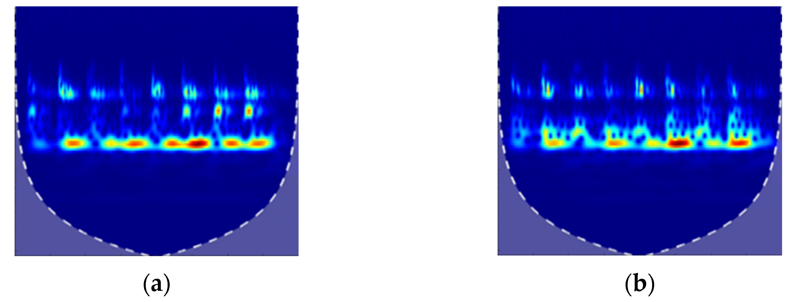
2.1. Signal Processing Techniques
2.2. Classification Algorithms
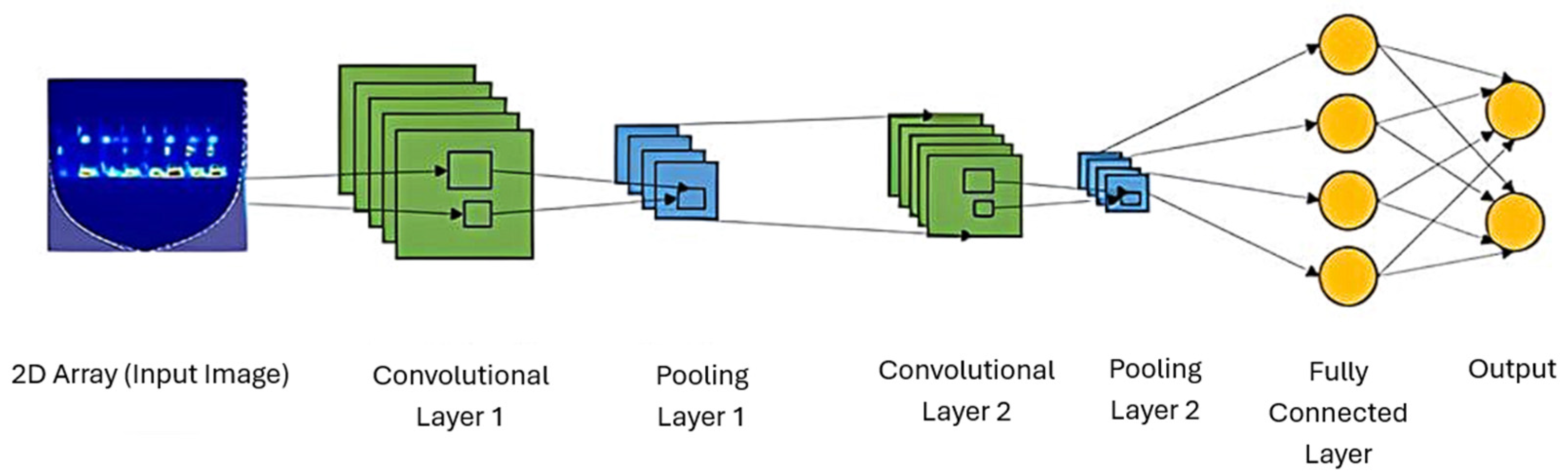
2.2.1. Convolutional Neural Networks
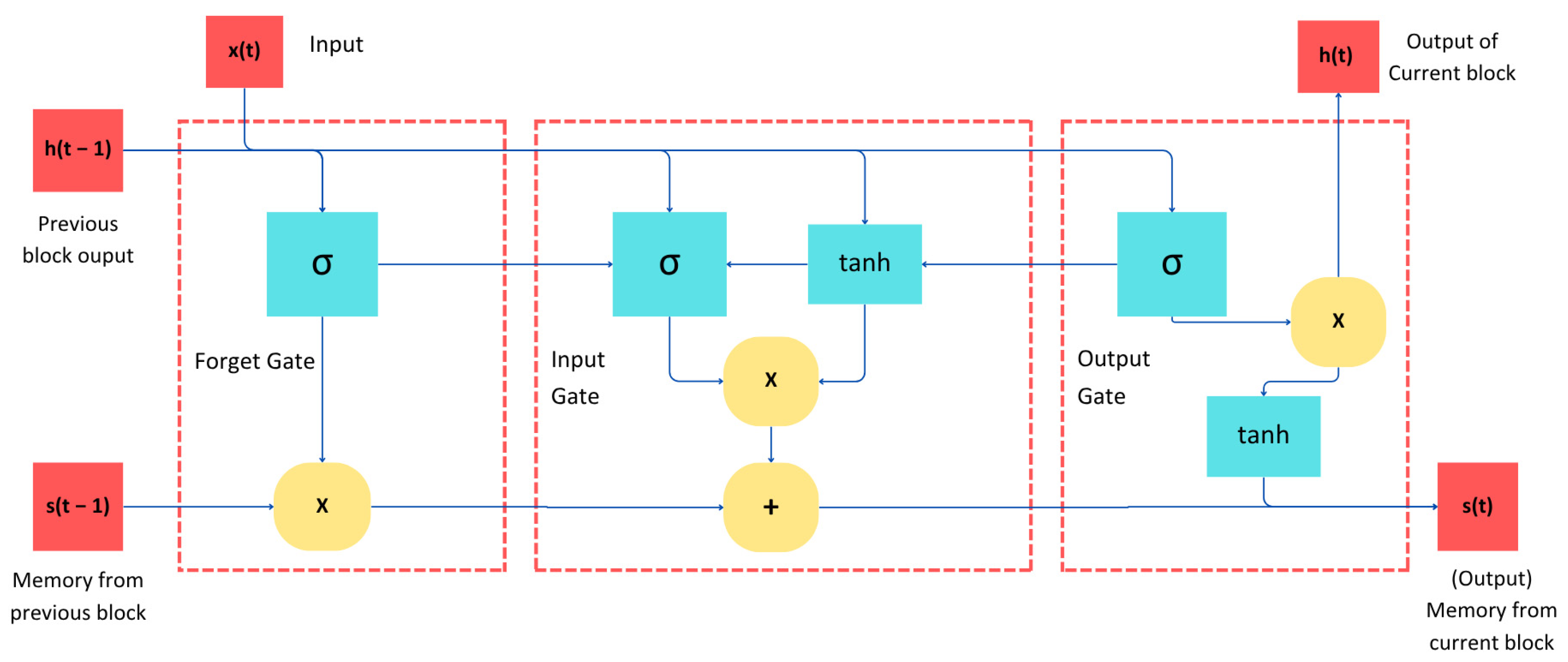
2.2.2. Long Short-Term Memory
2.2.3. Decision Trees and Random Forest
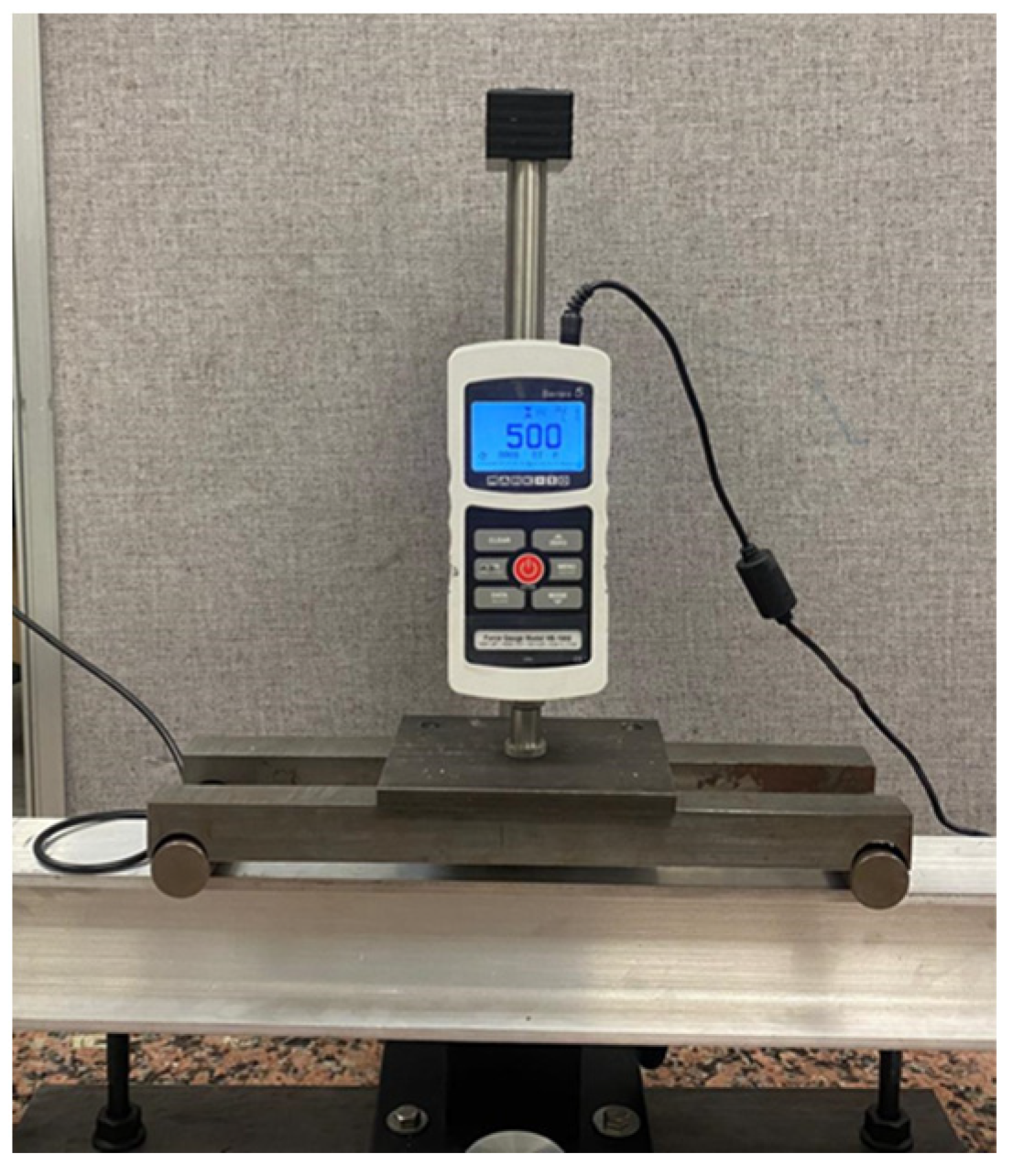
3. Materials and Methods
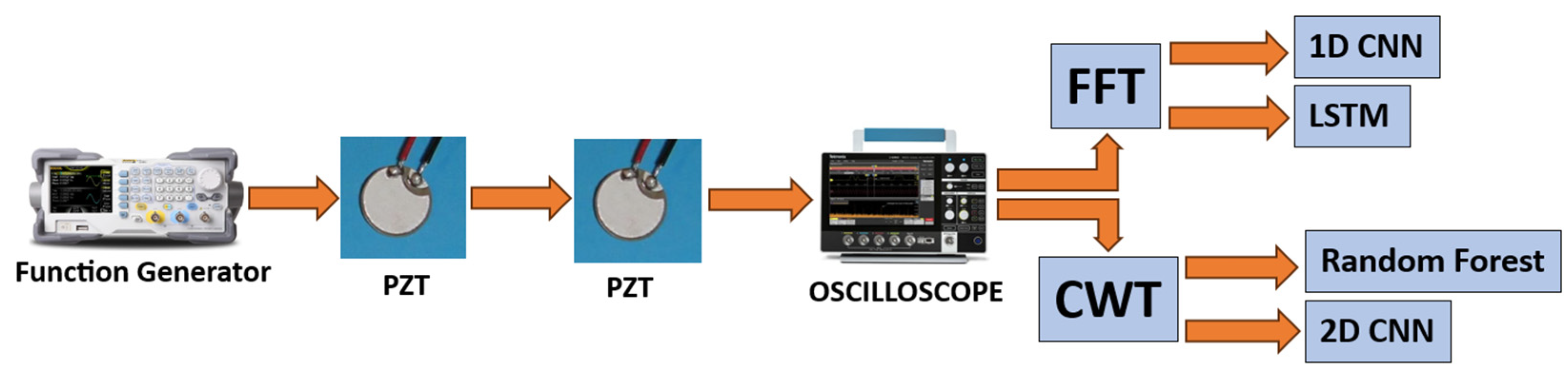
- PZT excitation–PZT monitoring: PZT attached to the left side of the beam. A Rigol DG 1022 function generator excited the PZT with a swept sine wave in the 100 kHz to 400 kHz range. The data were collected at a 1.25 GS/s frequency sampling rate.
- UCT probe excitation–PZT monitoring: The same method as above was implemented using an Olympus EPOCH 650 portable ultrasonic flaw detector with the UCT probe at a frequency of 250 kHz and sampling frequency of 0.625 GS/s Hz.
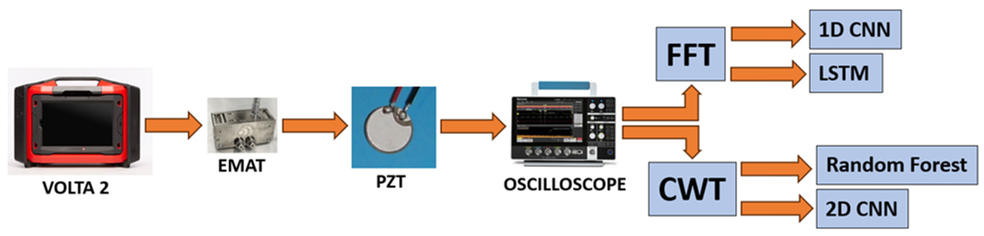
- EMAT probe excitation–PZT monitoring: Volta 2, a high-powered portable ultrasonic instrument, was used in conjunction with an EMAT probe to excite Point A and Point B on the beam at a frequency of 1150 kHz. The data were collected at a sampling frequency of 2.5 GS/s.
4. Results
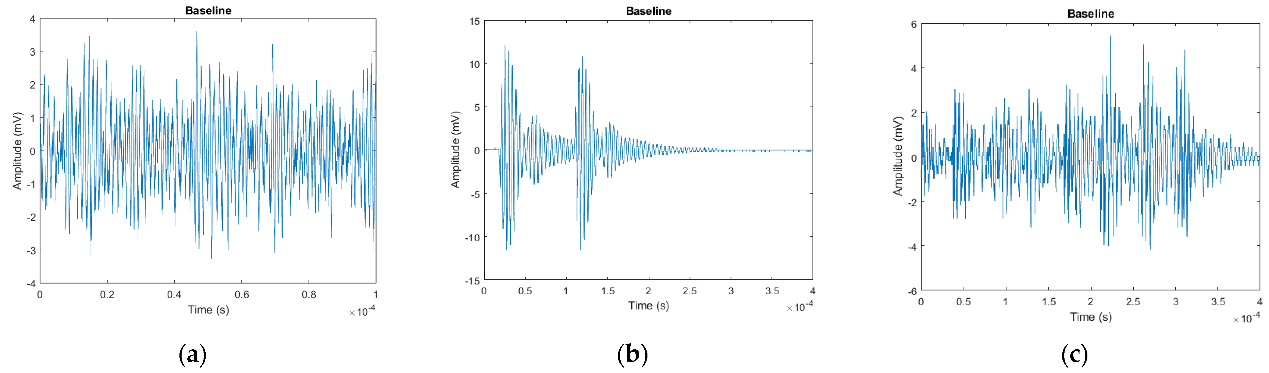
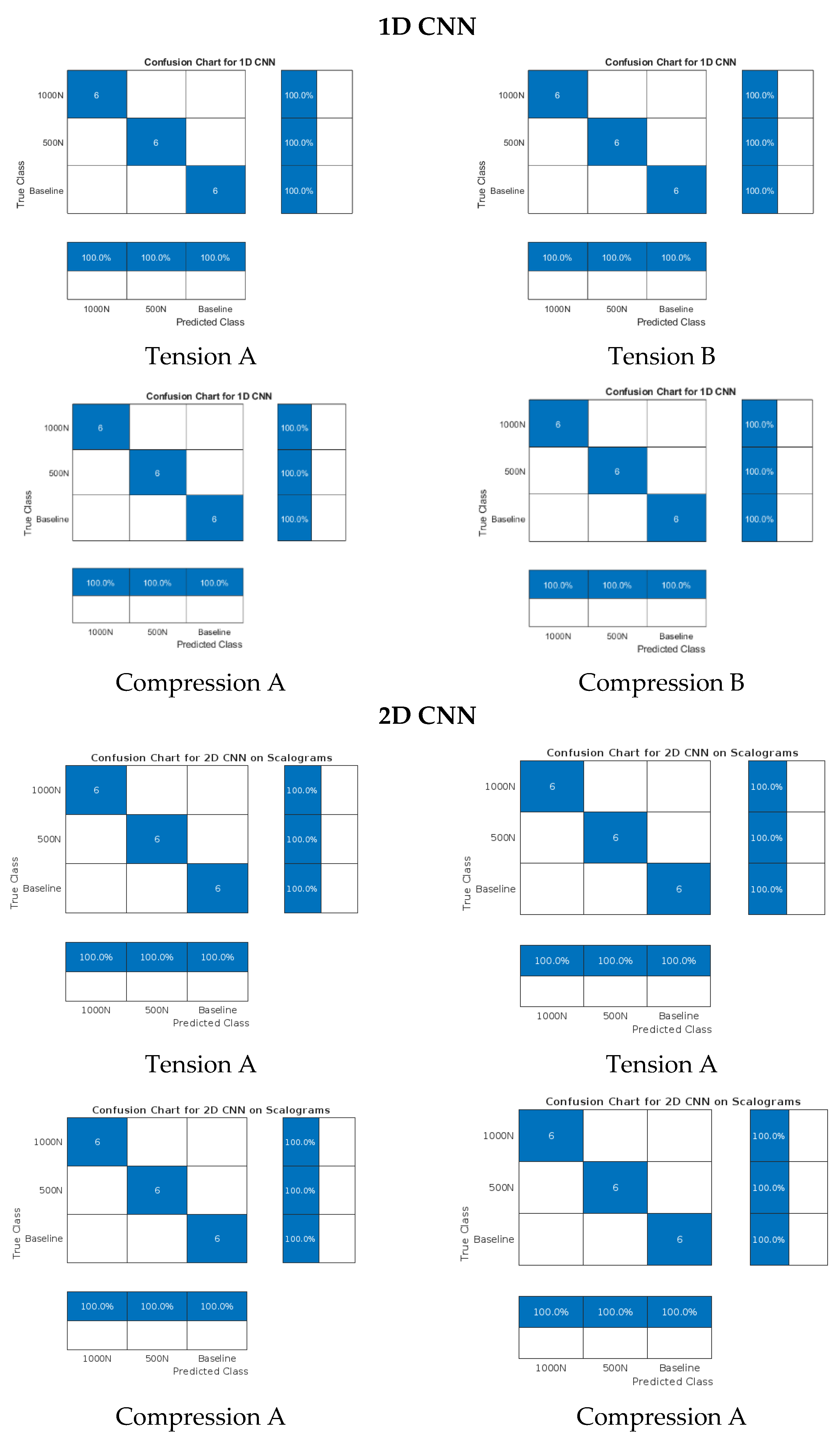
4.1. PZT Excitation–PZT Monitoring (PZT-PZT)
4.2. UCT Probe Excitation–PZT Monitoring (UCT-PZT)
4.3. EMAT Probe Excitation–PZT Monitoring (EMAT-PZT)
5. Discussion
6. Conclusions
Author Contributions
Funding
Data Availability Statement
Conflicts of Interest
Abbreviations
| SHM | Structural Health Monitoring |
| NDT | Non-Destructive Testing |
| PZT | Piezoelectric Transducer |
| CNN | Convolutional Neural Network |
| 1D CNN | One-Dimensional Convolutional Neural Network |
| 2D CNN | Two-Dimensional Convolutional Neural Network |
| FFT | Fast Fourier Transform |
| CWT | Continuous Wavelet Transform |
| UCT | Ultrasonic Contact Transducer |
| EMAT | Electromagnetic Acoustic Transducer |
| AI | Artificial Intelligence |
References
- Xanthakos, P.P. Theory and Design of Bridges; John Wiley & Sons: Hoboken, NJ, USA, 1994. [Google Scholar]
- Pallarés, F.J.; Betti, M.; Bartoli, G.; Pallarés, L. Structural health monitoring (SHM) and Nondestructive testing (NDT) of slender masonry structures: A practical review. Constr. Build. Mater. 2021, 297, 123768. [Google Scholar] [CrossRef]
- Di Lorenzo, G.; Formisano, A.; Landolfo, R. On the Origin of I Beams and Quick Analysis on the Structural Efficiency of Hot-rolled Steel Members. Open Civ. Eng. J. 2017, 11, 332–344. [Google Scholar] [CrossRef]
- Hussain, B. Integration of Non-Destructive Testing Techniques and Machine Learning Algorithms for Enhanced Structural Health Monitoring of Bridges. Curr. J. Appl. Sci. Technol. 2024, 43, 20–31. [Google Scholar] [CrossRef]
- Mehrabi, A.; Dolati, S.; Malla, P.; Farhangdoust, S.; Azzi, Z. Non-Destructive Testing for Inspection of Bridges and Buildings; Cambridge Scholars Publishing: Newcastle upon Tyne, UK, 2025. [Google Scholar]
- Li, X.; Shi, D.; Yu, Z. Nondestructive Damage Testing of Beam Structure Based on Vibration Response Signal Analysis. Materials 2020, 13, 3301. [Google Scholar] [CrossRef] [PubMed]
- Baba, S.; Kondoh, J. Damage evaluation of fixed beams at both ends for bridge health monitoring using a combination of a vibration sensor and a surface acoustic wave device. Eng. Struct. 2022, 262, 114323. [Google Scholar] [CrossRef]
- Mehrabi, A.; Dolati, S.S.K. Structural Health Monitoring and Performance Evaluation of Bridges and Structural Elements. Infrastructures 2024, 9, 178. [Google Scholar] [CrossRef]
- Fahr, A. Aeronautical Applications of Non-Destructive Testing; DEStech Publications, Inc.: Lancaster, PA, USA, 2013. [Google Scholar]
- Büyüköztürk, O.; Taşdemir, M.A. Nondestructive Testing of Materials and Structures; Springer Science & Business Media: Berlin, Germany, 2012. [Google Scholar]
- Blitz, J.; Simpson, G. Ultrasonic Methods of Non-Destructive Testing; Springer Science & Business Media: Berlin, Germany, 1995. [Google Scholar]
- Bolborea, B.; Baeră, C.; Gruin, A.; Vasile, A.-C.; Barbu, A.-M. A review of non-destructive testing methods for structural health monitoring of earthen constructions. Alex. Eng. J. 2025, 114, 55–81. [Google Scholar] [CrossRef]
- Nguyen, Q.-B.; Nguyen, H.-H. An Efficient Approach for Damage Identification of Beams Using Mid-Span Static Deflection Changes. Eng 2024, 5, 895–917. [Google Scholar] [CrossRef]
- Hassani, S.; Dackermann, U. A Systematic Review of Advanced Sensor Technologies for Non-Destructive Testing and Structural Health Monitoring. Sensors 2023, 23, 2204. [Google Scholar] [CrossRef]
- Goggin, P.; Huang, J.; White, E.; Haugse, E. Challenges for SHM transition to future aerospace systems. In Proceedings of the 4th International Workshop on Structural Health Monitoring: From Diagnostics and Prognostics to Structural Health Management, Standford, CA, USA, 15–17 September 2003; DEStech Publications: Lancaster, PA, USA, 2003; pp. 30–41. [Google Scholar]
- Liu, Z. Smart Sensors for Structural Health Monitoring and Nondestructive Evaluation. Sensors 2024, 24, 603. [Google Scholar] [CrossRef]
- Mei, H.; Haider, M.F.; Joseph, R.; Migot, A.; Giurgiutiu, V. Recent Advances in Piezoelectric Wafer Active Sensors for Structural Health Monitoring Applications. Sensors 2019, 19, 383. [Google Scholar] [CrossRef] [PubMed]
- Gibson, A.; Popovics, J.S. Lamb Wave Basis for Impact-Echo Method Analysis. J. Eng. Mech. 2005, 131, 438–443. [Google Scholar] [CrossRef]
- Na, W.S.; Baek, J. A Review of the Piezoelectric Electromechanical Impedance Based Structural Health Monitoring Technique for Engineering Structures. Sensors 2018, 18, 1307. [Google Scholar] [CrossRef]
- Falcetelli, F.; Venturini, N.; Romero, M.B.; Martinez, M.J.; Pant, S.; Troiani, E. Broadband signal reconstruction for SHM: An experimental and numerical time reversal methodology. J. Intell. Mater. Syst. Struct. 2021, 32, 1043–1058. [Google Scholar] [CrossRef]
- Khodaei, Z.S.; Grigg, S. Aerospace Requirements. In Structural Health Monitoring Damage Detection Systems for Aerospace; Springer: Cham, Switzerland, 2021; p. 73. [Google Scholar]
- Bradfield, G. Improvements in ultrasonic flaw detection. J. Br. Inst. Radio Eng. 1954, 14, 303–308. [Google Scholar] [CrossRef]
- Robertson, D.; Camps, O.; Mayer, J.; Gish, W. Wavelets and electromagnetic power system transients. IEEE Trans. Power Deliv. 1996, 11, 1050–1058. [Google Scholar] [CrossRef]
- Ghazali, K.H.; Mansor, M.F.; Mustafa, M.M.; Hussain, A. Feature extraction technique using discrete wavelet transform for image classification. In Proceedings of the 5th Student Conference on Research and Development, Selangor, Malaysia, 11–12 December 2007; IEEE: Piscataway, NJ, USA, 2007; pp. 1–4. [Google Scholar]
- Aguiar-Conraria, L.; Soares, M.J. The Continuous Wavelet Transform: A Primer; NIPE-Universidade do Minho: Braga, Portugal, 2011. [Google Scholar]
- Thakral, S.; Manhas, P. Image processing by using different types of discrete wavelet transform. In Proceedings of the Advanced Informatics for Computing Research: Second International Conference, ICAICR 2018, Shimla, India, 14–15 July 2018; Revised Selected Papers, Part I 2. Springer: Cham, Switzerland, 2019; pp. 499–507. [Google Scholar]
- Kammler, D.W. A First Course in Fourier Analysis; Cambridge University Press: Cambridge, UK, 2007. [Google Scholar]
- Zhang, Q.; Barri, K.; Babanajad, S.K.; Alavi, A.H. Real-Time Detection of Cracks on Concrete Bridge Decks Using Deep Learning in the Frequency Domain. Engineering 2021, 7, 1786–1796. [Google Scholar] [CrossRef]
- Kiranyaz, S.; Avci, O.; Abdeljaber, O.; Ince, T.; Gabbouj, M.; Inman, D.J. 1D convolutional neural networks and applications: A survey. Mech. Syst. Signal Process. 2021, 151, 107398. [Google Scholar] [CrossRef]
- Azizjon, M.; Jumabek, A.; Kim, W. 1D CNN based network intrusion detection with normalization on imbalanced data. In Proceedings of the 2020 International Conference on Artificial Intelligence in Information and Communication (ICAIIC), Fukuoka, Japan, 19–21 February 2020; IEEE: Piscataway, NJ, USA, 2020; pp. 218–224. [Google Scholar]
- Zhao, J.; Mao, X.; Chen, L. Speech emotion recognition using deep 1D & 2D CNN LSTM networks. Biomed. Signal Process. Control. 2019, 47, 312–323. [Google Scholar]
- Yu, C.; Han, R.; Song, M.; Liu, C.; Chang, C.-I. A Simplified 2D-3D CNN Architecture for Hyperspectral Image Classification Based on Spatial–Spectral Fusion. IEEE J. Sel. Top. Appl. Earth Obs. Remote Sens. 2020, 13, 2485–2501. [Google Scholar] [CrossRef]
- Chang, J.; Sha, J. An efficient implementation of 2D convolution in CNN. IEICE Electron. Express 2017, 14, 20161134. [Google Scholar] [CrossRef]
- Kumar, J.; Goomer, R.; Singh, A.K. Long Short Term Memory Recurrent Neural Network (LSTM-RNN) Based Workload Forecasting Model for Cloud Datacenters. Procedia Comput. Sci. 2018, 125, 676–682. [Google Scholar] [CrossRef]
- Ji, H.; Lou, Y.; Cheng, S.; Xie, Z.; Zhu, L. An Advanced Long Short-Term Memory (LSTM) Neural Network Method for Predicting Rate of Penetration (ROP). ACS Omega 2022, 8, 934–945. [Google Scholar] [CrossRef] [PubMed]
- Rokach, L.; Maimon, O. Decision trees. In Data Mining and Knowledge Discovery Handbook; Springer: New York, NY, USA, 2005; pp. 165–192. [Google Scholar]
- Ali, J.; Khan, R.; Ahmad, N.; Maqsood, I. Random forests and decision trees. Int. J. Comput. Sci. Issues IJCSI 2012, 9, 272. [Google Scholar]
- Breiman, L. Random Forests. Mach. Learn. 2001, 45, 5–32. [Google Scholar] [CrossRef]
- Hasni, H.; Jiao, P.; Alavi, A.H.; Lajnef, N.; Masri, S.F. Structural health monitoring of steel frames using a network of self-powered strain and acceleration sensors: A numerical study. Autom. Constr. 2018, 85, 344–357. [Google Scholar] [CrossRef]
- Altabey, W.A.; Noori, M.; Wu, Z.; Silik, A.; Sarhosis, V. Enhancement of structural health monitoring framework on beams based on k-nearest neighbor algorithm. In Proceedings of the 14th International Workshop on Structural Health Monitoring, Stanford, CA, USA, 12–14 September 2023. [Google Scholar]
- Achouri, F.; Khatir, A.; Smahi, Z.; Capozucca, R.; Brahim, A.O. Structural health monitoring of beam model based on swarm intelligence-based algorithms and neural networks employing FRF. J. Braz. Soc. Mech. Sci. Eng. 2023, 45, 621. [Google Scholar] [CrossRef]
- Buljak, V.; Cocchetti, G.; Cornaggia, A.; Maier, G. Assessment of residual stresses and mechanical characterization of materials by “hole drilling” and indentation tests combined and by inverse analysis. Mech. Res. Commun. 2015, 68, 18–24. [Google Scholar] [CrossRef]


| Algorithm | Strengths | Weaknesses | Best Use Case |
|---|---|---|---|
| 1D CNN | Efficient for time-series data; low computational cost. | Limited spatial feature extraction. | Analysis of raw sensor signals. |
| 2D CNN | Captures spatial features; ideal for spectrograms. | High computational demands; requires large datasets. | Spectrogram analysis from SHM signals. |
| LSTM | Model long-term dependencies; good for sequential data. | Computationally intensive; sensitive to tuning. | Time-series prediction and trend analysis. |
| Decision Tree | Simple, interpretable; low computational cost. | Prone to overfitting; struggles with complex patterns. | Quick and interpretable classifications. |
| Random Forest | Robust; reduces overfitting; handles high-dimensional data. | High memory usage; less interpretable. | Comprehensive SHM classification tasks. |
| Signal Processing and Classification Algorithm | Tension | Compression | ||
|---|---|---|---|---|
| A | B | A | B | |
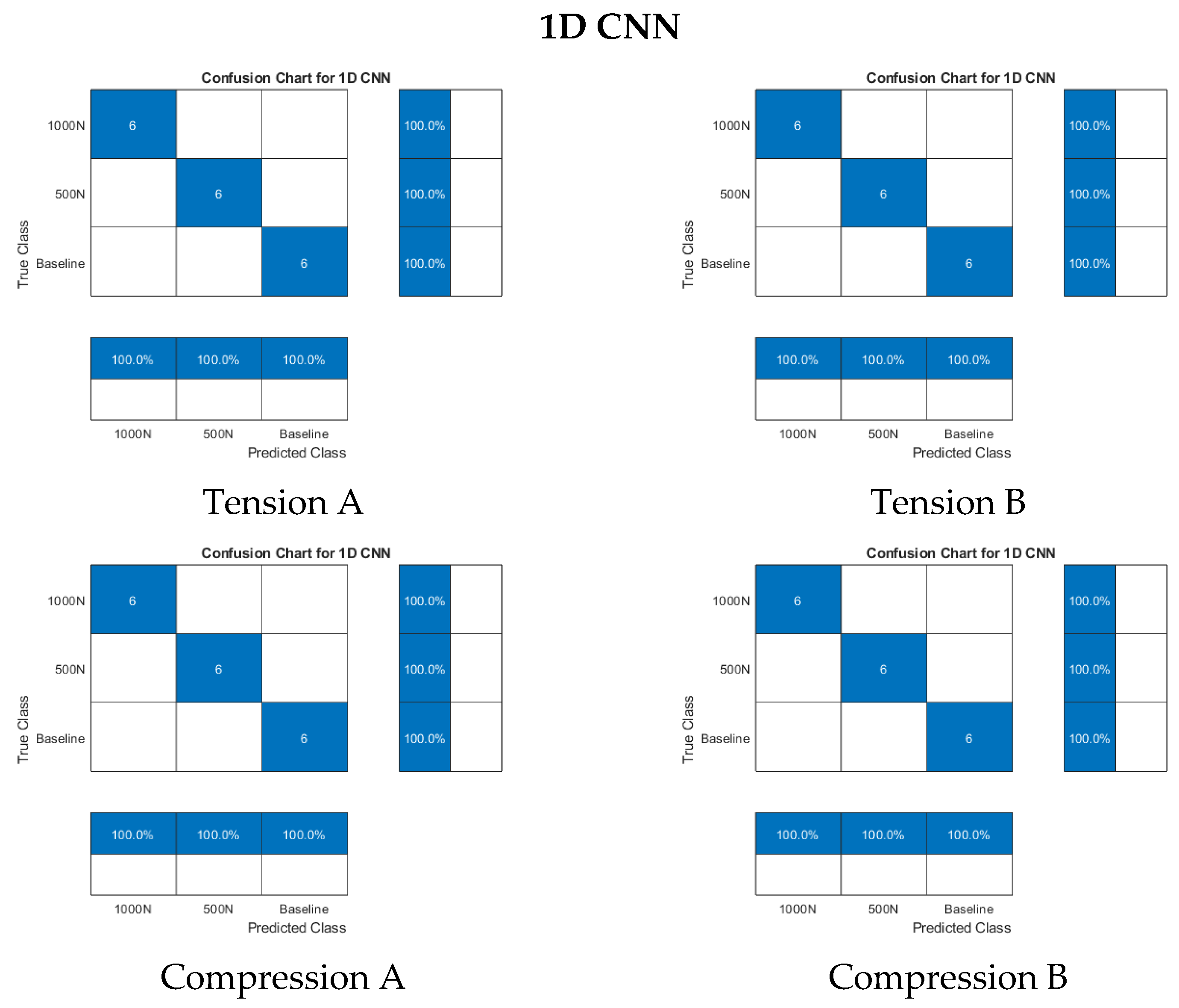
| FFT–1D-CNN | 100% | 100% | 100% | 100% |
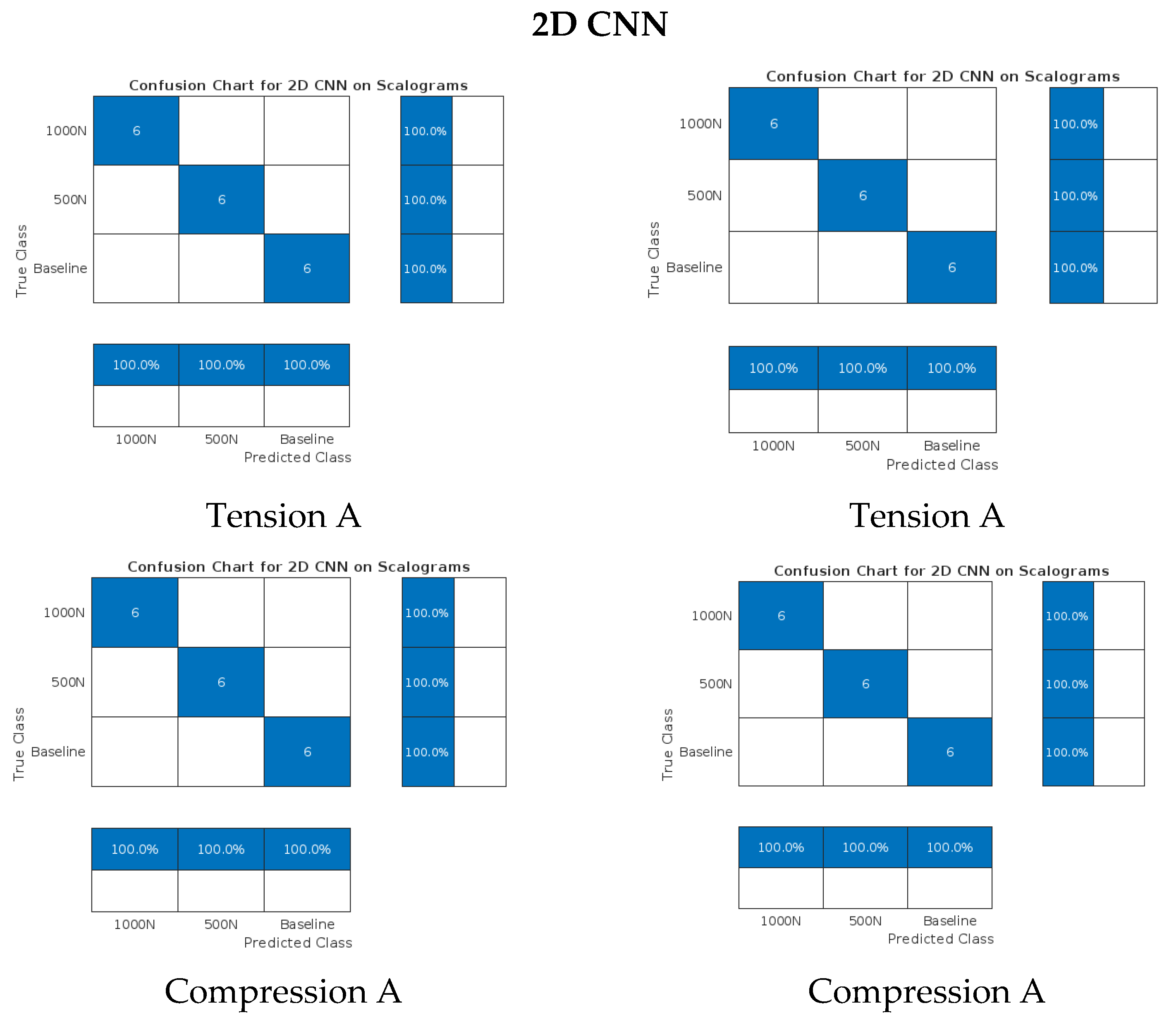
| CWT–2D CNN | 100% | 100% | 100% | 100% |
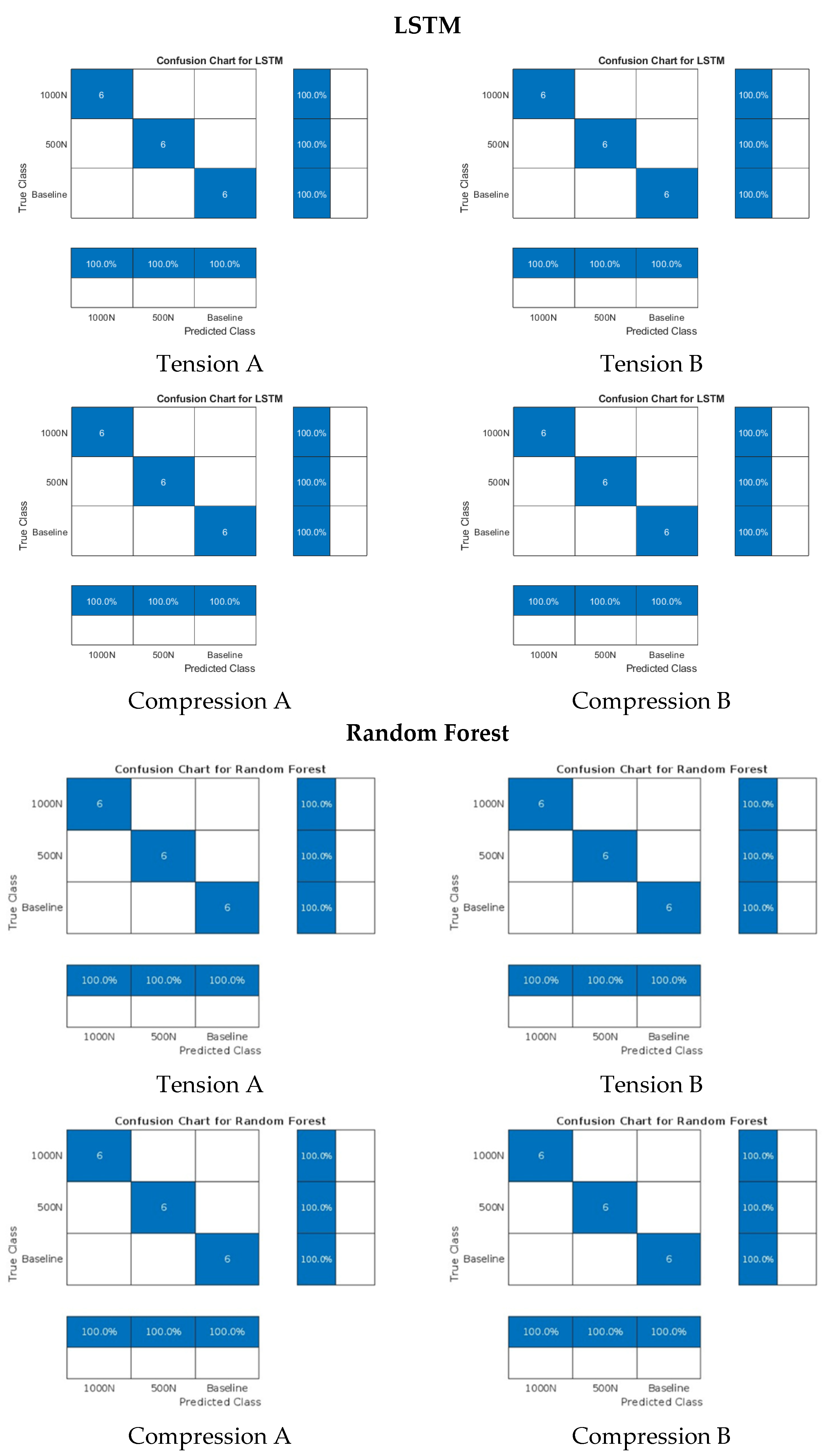
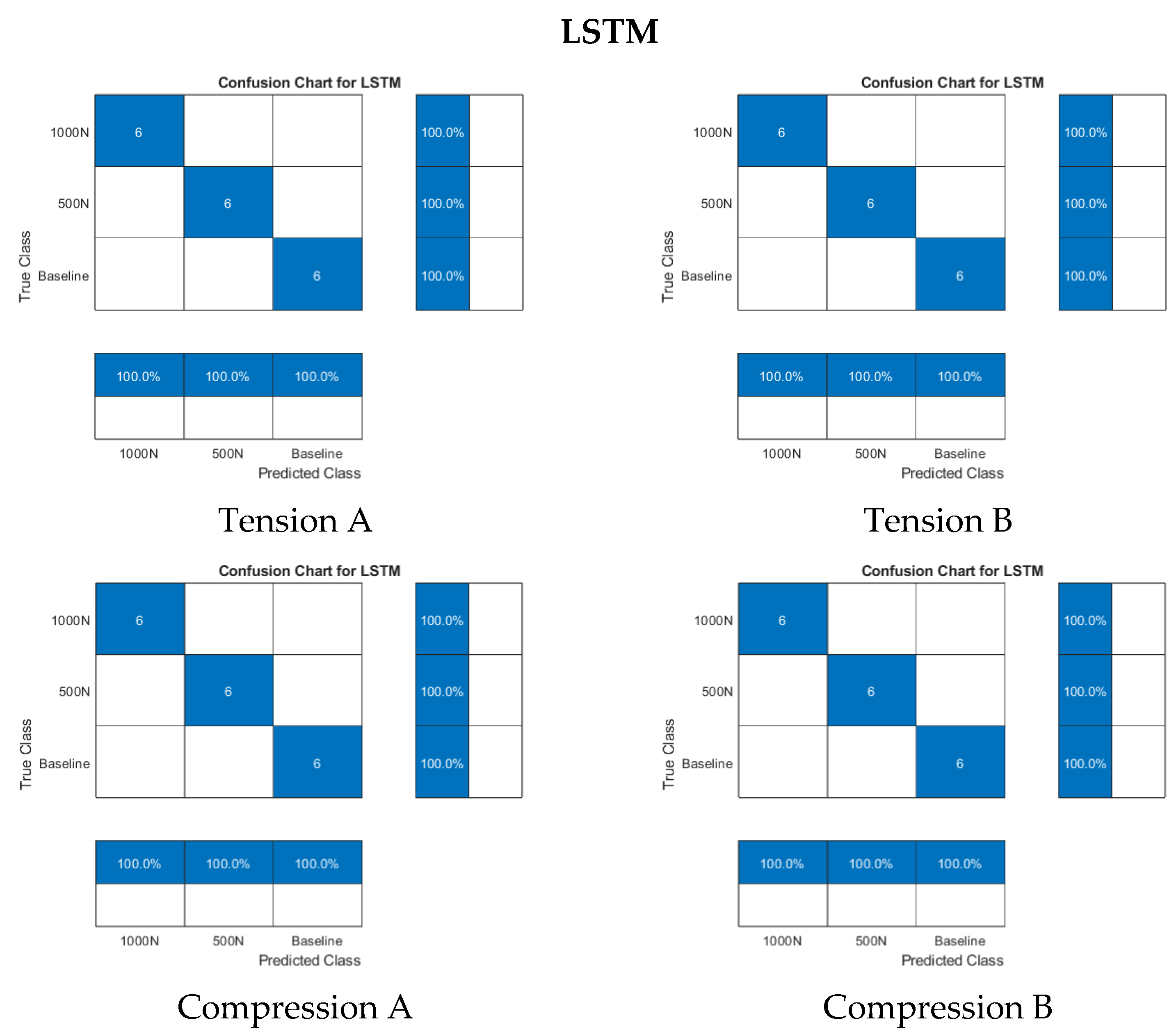
| FFT–LSTM | 100% | 100% | 100% | 100% |
| CWT–Random Forest | 100% | 100% | 100% | 100% |
| Signal Processing and Classification Algorithm | Tension | Compression | ||
|---|---|---|---|---|
| A | B | A | B | |
| FFT–1D CNN | 100% | 100% | 100% | 100% |
| CWT–2D CNN | 100% | 100% | 100% | 100% |
| FFT–LSTM | 100% | 100% | 100% | 100% |
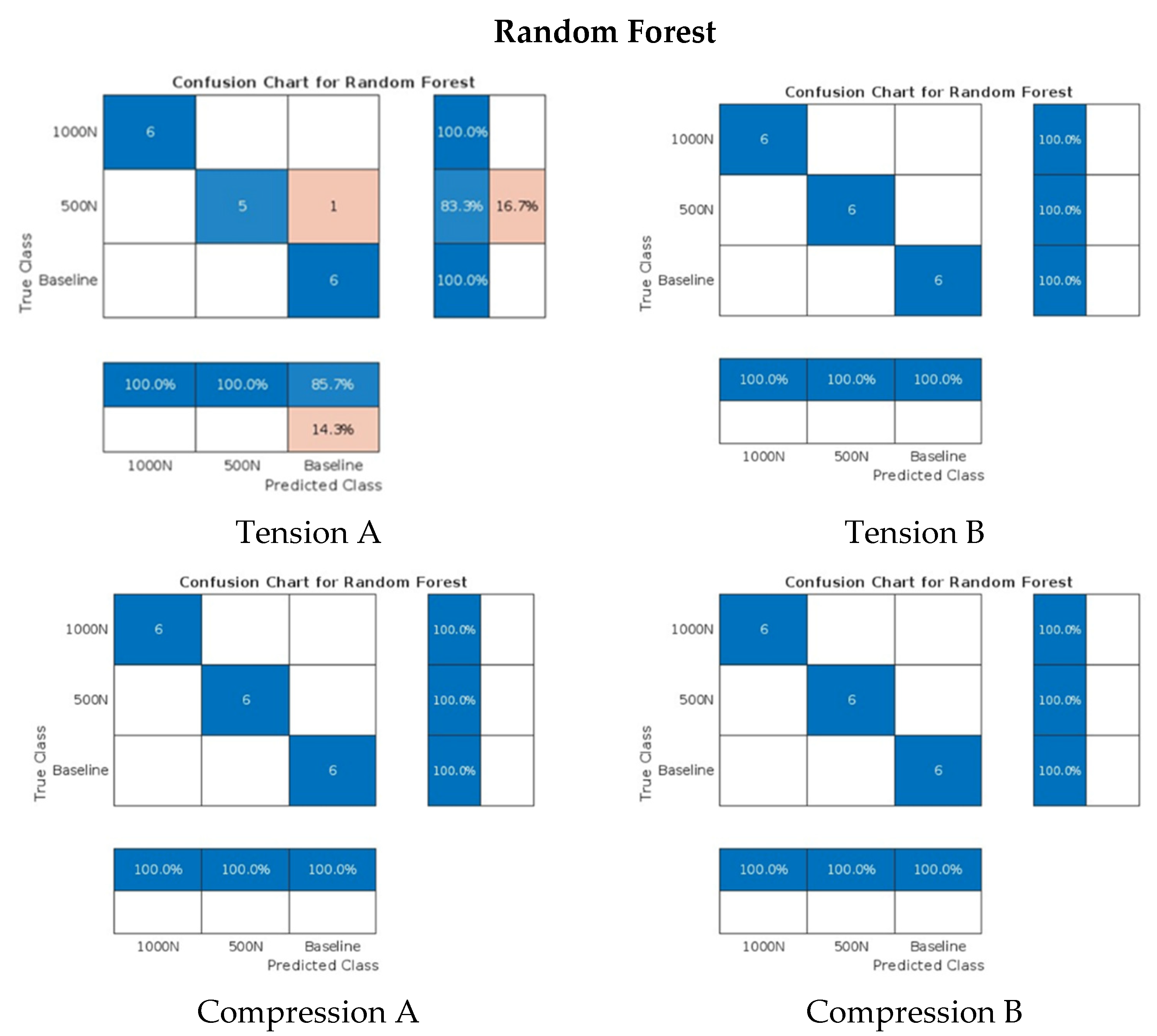
| CWT–Random Forest | 94% | 100% | 100% | 100% |
| Signal Processing and Classification Algorithm | Tension | Compression | ||
|---|---|---|---|---|
| A | B | A | B | |
| FFT–1D CNN | 100% | 100% | 100% | 100% |
| CWT–2D CNN | 100% | 100% | 100% | 100% |
| FFT–LSTM | 100% | 100% | 100% | 100% |
| CWT–Random Forest | 100% | 100% | 100% | 100% |
Disclaimer/Publisher’s Note: The statements, opinions and data contained in all publications are solely those of the individual author(s) and contributor(s) and not of MDPI and/or the editor(s). MDPI and/or the editor(s) disclaim responsibility for any injury to people or property resulting from any ideas, methods, instructions or products referred to in the content. |
© 2025 by the authors. Licensee MDPI, Basel, Switzerland. This article is an open access article distributed under the terms and conditions of the Creative Commons Attribution (CC BY) license (https://creativecommons.org/licenses/by/4.0/).
Share and Cite
Byfield, R.; Shabaka, A.; Molina Vargas, M.; Tansel, I. Intelligent Hybrid SHM-NDT Approach for Structural Assessment of Metal Components. Infrastructures 2025, 10, 174. https://doi.org/10.3390/infrastructures10070174
Byfield R, Shabaka A, Molina Vargas M, Tansel I. Intelligent Hybrid SHM-NDT Approach for Structural Assessment of Metal Components. Infrastructures. 2025; 10(7):174. https://doi.org/10.3390/infrastructures10070174
Chicago/Turabian StyleByfield, Romaine, Ahmed Shabaka, Milton Molina Vargas, and Ibrahim Tansel. 2025. "Intelligent Hybrid SHM-NDT Approach for Structural Assessment of Metal Components" Infrastructures 10, no. 7: 174. https://doi.org/10.3390/infrastructures10070174
APA StyleByfield, R., Shabaka, A., Molina Vargas, M., & Tansel, I. (2025). Intelligent Hybrid SHM-NDT Approach for Structural Assessment of Metal Components. Infrastructures, 10(7), 174. https://doi.org/10.3390/infrastructures10070174