
Hybrid Adaptive Sheep Flock Optimization and Gradient Descent Optimization for Energy Management in a Grid-Connected Microgrid

 ,
,  ,
, 
Abstract
1. Introduction
- This work contributes in the following ways:
- This study thoroughly examines a range of strategies that efficiently manage uncertainties and reduce power imbalances in the context of renewable energy sources. Each strategy is thoroughly examined, including in-depth evaluations and recommendations for EM in situations when there are significant disparities between power generation and demand.
- Improves the solution accuracy and convergence speed by leveraging the strengths of both methods, i.e., ASFO and GDO, and optimizes the scheduling of distributed generation units and grid exchange under uncertain PV and wind conditions.
- Further, it demonstrates faster and more accurate solution discovery compared to traditional methods like GDO, B&B, interior point optimization, and Golden Jackal optimization to validate its effectiveness.
- At last, addressed the impact of DOS attacks, FDI attacks, and the presence of outliers on operational expenditure and also considered the uncertainties in PV, WT, and load demand.
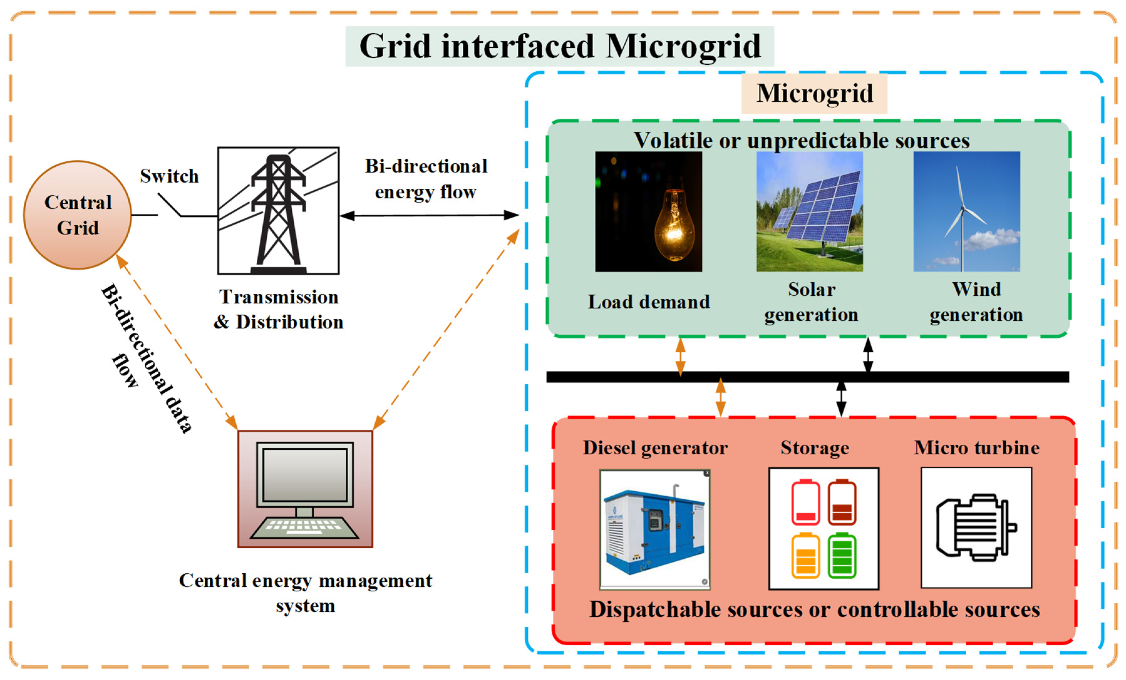
2. Microgrid Modeling
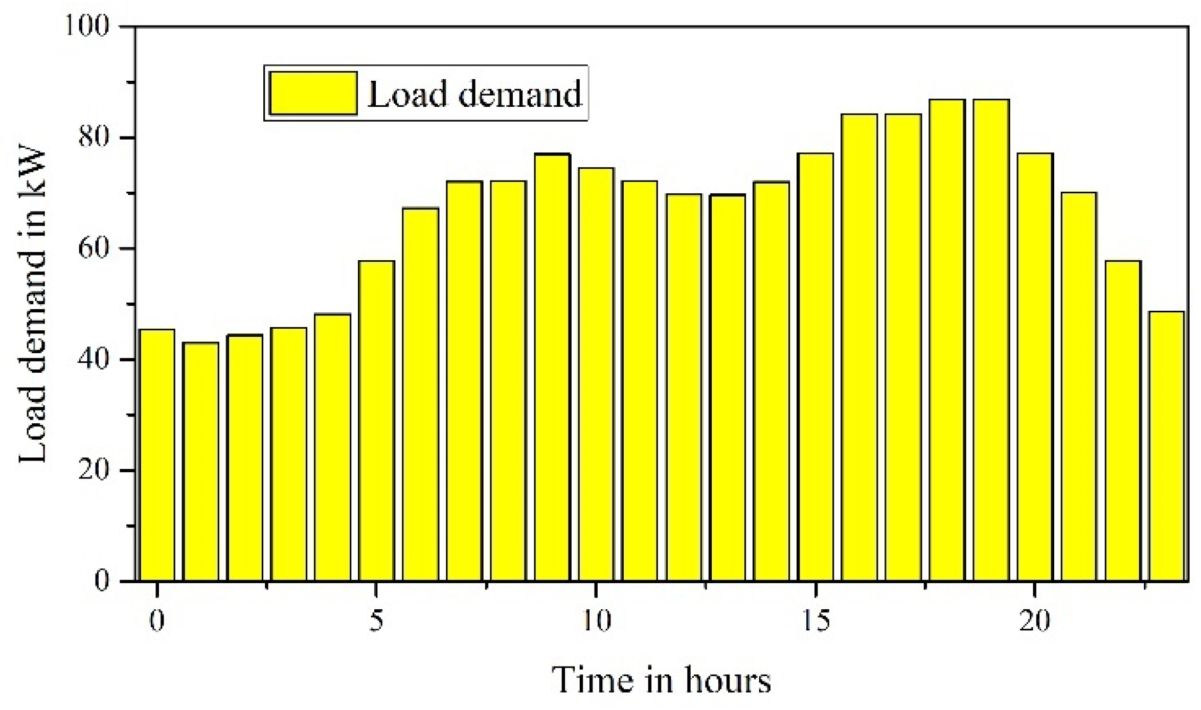
2.1. Non-Dispatchable Sources
2.2. Dispatchable Sources
2.2.1. Diesel Generators
2.2.2. Fuel Cell
2.2.3. Microturbine
3. Problem Formulation
3.1. Equality Constraint
3.2. Inequality Constraints
3.2.1. BESS Constraints [42]
3.2.2. Utility Constraints
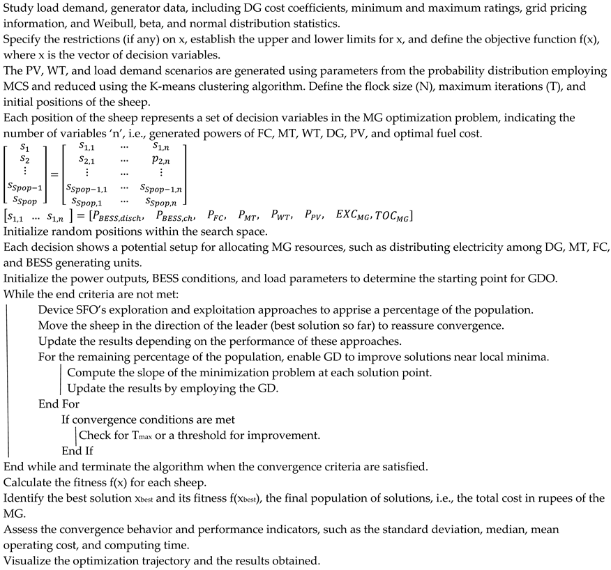
4. Proposed Methodology
4.1. Sheep Flock Optimization
4.1.1. Following Behavior
4.1.2. Scattering Behavior
4.1.3. Lamb Reunion
4.2. Shortcomings in SFO
4.3. Adaptive ASFO
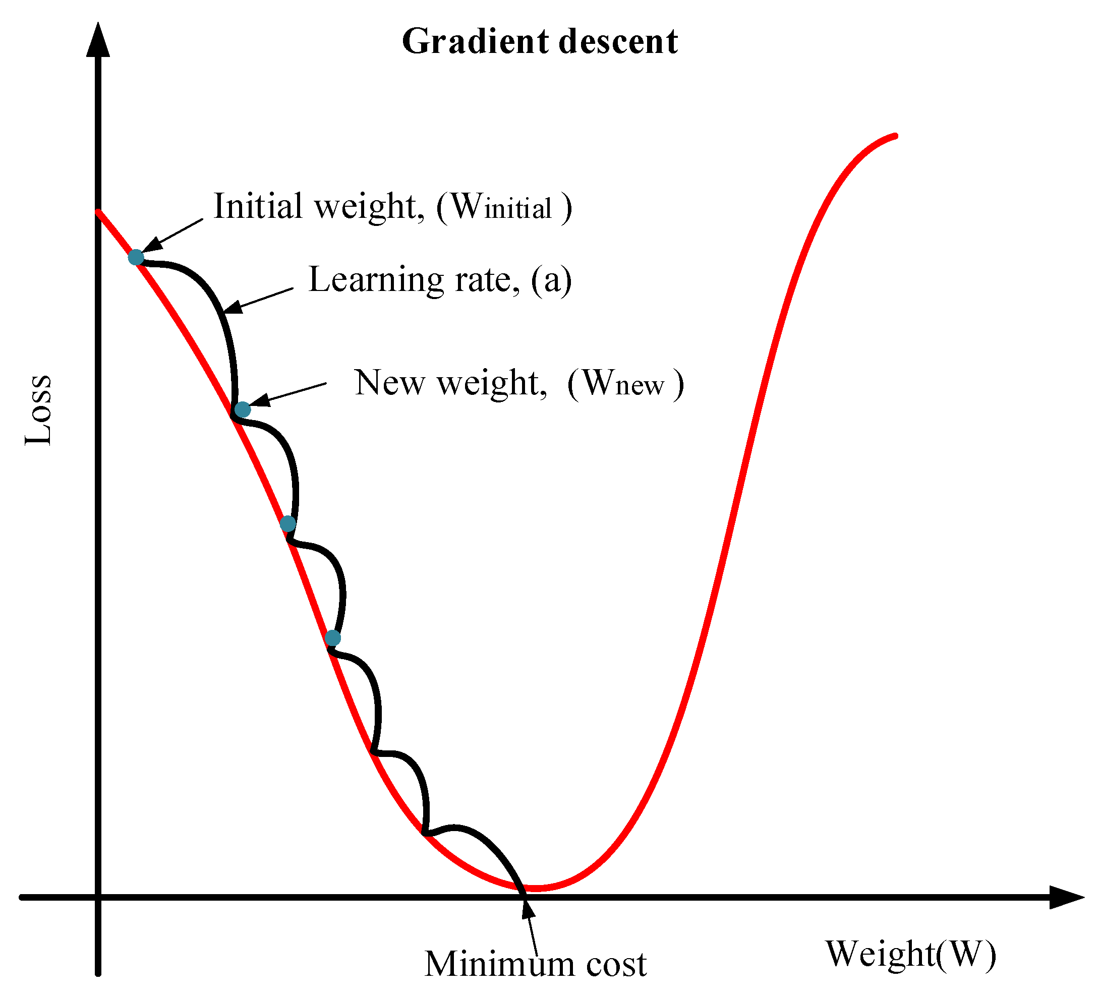
4.4. Gradient Descent Optimization
5. Results and Discussions
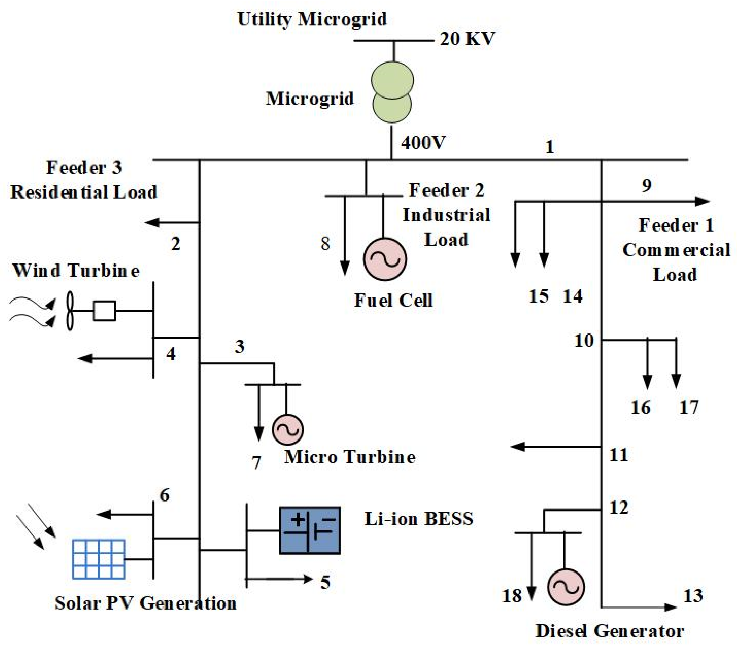
- Case 1: Application to an IEEE-18 bus system.
- Case 2: Application to a 33-bus radial distribution network.
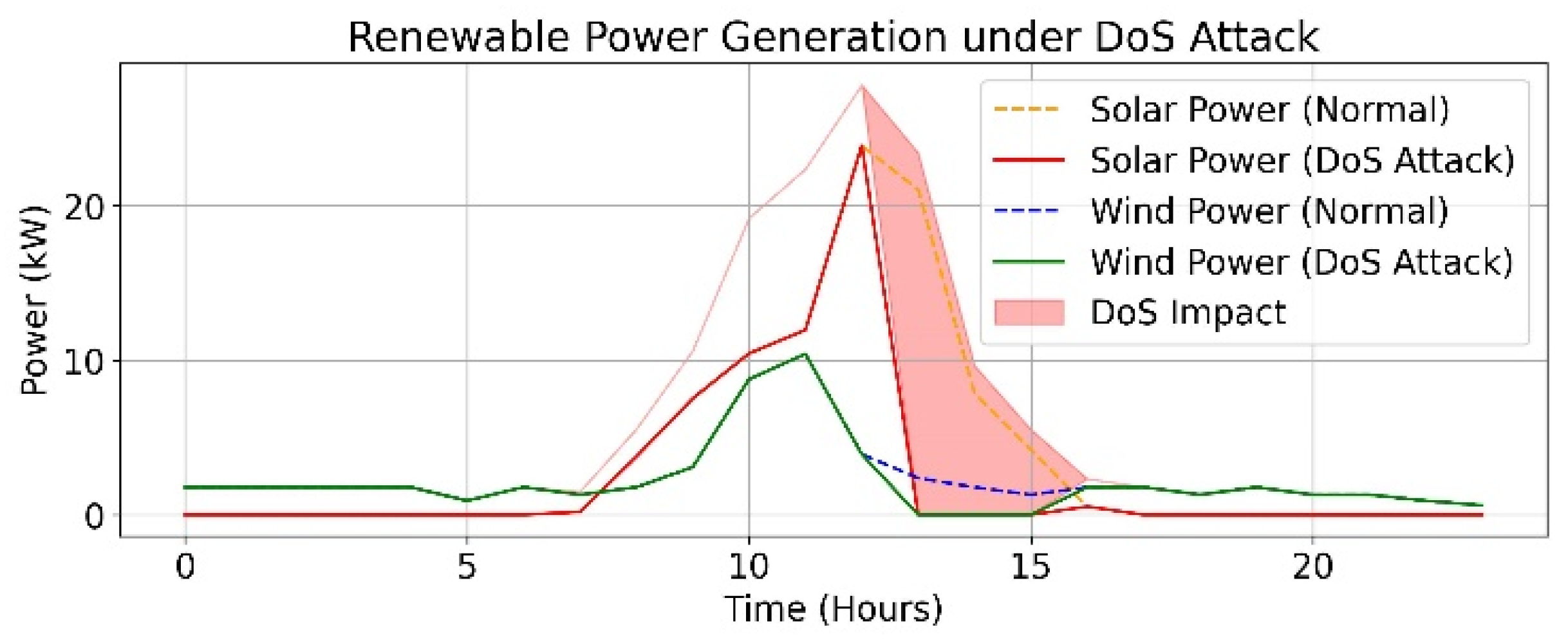
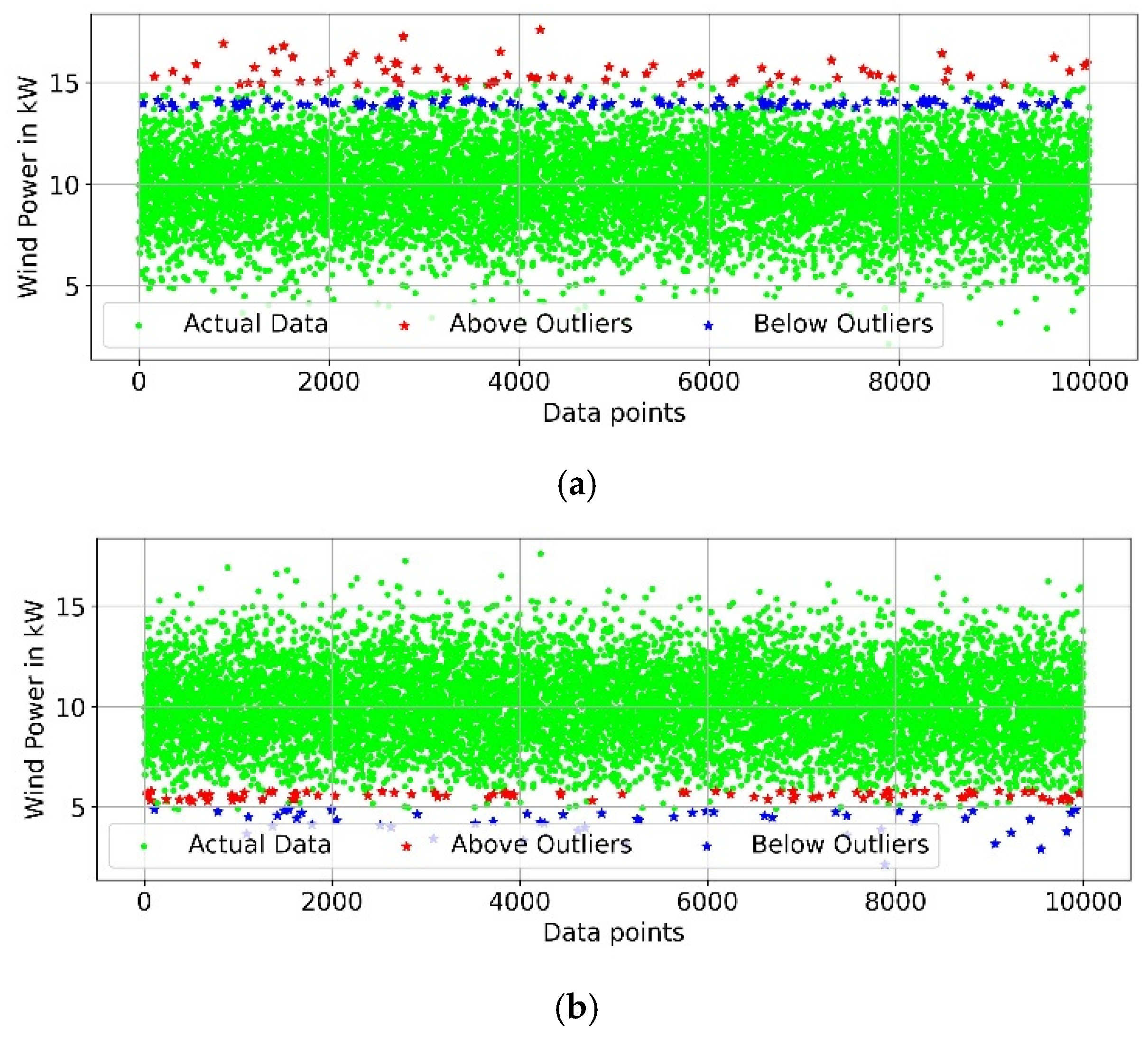
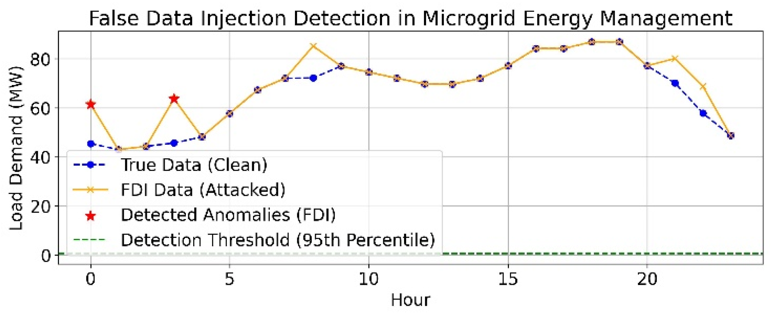
- Case 3: Impact of DOS attack and outliers on the operational expenditure.
6. Conclusions
Author Contributions
Funding
Data Availability Statement
Conflicts of Interest
References
- Ali, R.; Sajjad, F.; Mahmud, F.; Moein, M. Decentralized transactive energy management of multi-microgrid distribution systems based on ADMM. Int. J. Electr. Power Energy Syst. 2021, 132, 107126. [Google Scholar]
- Cao, Y. Optimal Energy Management for Multi-Microgrid Under a Transactive Energy Framework with Distributionally Robust Optimization. IEEE Trans. Smart Grid 2022, 13, 599–612. [Google Scholar] [CrossRef]
- Ma, W.; Wang, J.; Gupta, V.; Chen, C. Distributed Energy Management for Networked MG Using Online ADMM with Regret. IEEE Trans. Smart Grid 2018, 9, 847–856. [Google Scholar] [CrossRef]
- Liu, Y.; Beng Gooi, H.; Xin, H. Distributed energy management for the multi-microgrid system based on ADMM. In Proceedings of the 2017 IEEE Power & Energy Society General Meeting, Chicago, IL, USA, 16–20 July 2017; pp. 1–5. [Google Scholar]
- Zheng, Y.; Song, Y.; Hill, D.J.; Zhang, Y. Multiagent System Based Microgrid Energy Management via Asynchronous Consensus ADMM. IEEE Trans. Energy Convers. 2018, 33, 886–888. [Google Scholar] [CrossRef]
- Zhao, D. Differential Privacy Energy Management for Islanded Microgrids with Distributed Consensus-Based ADMM Algorithm. IEEE Trans. Control. Syst. Technol. 2023, 31, 1018–1031. [Google Scholar] [CrossRef]
- Leeuwen, G.; AlSkaif, T.; Gibescu, M.; van Sark, W. An integrated blockchain-based energy management platform with bilateral trading for microgrid communities. Appl. Energy 2020, 263, 114613. [Google Scholar] [CrossRef]
- Amjad Anvari, M.; Alireza, S.; Taher, N.; Mohammad, P. Multi-objective operation management of a renewable MG (micro-grid) with back-up micro-turbine/fuel cell/battery hybrid power source. Energy 2011, 36, 6490–6507. [Google Scholar]
- Nikmehr, N.; Najafi-Ravadanegh, S. Optimal operation of distributed generations in micro-grids under uncertainties in load and renewable power generation using heuristic algorithm. IET Renew. Power Gener. 2019, 9, 982–990. [Google Scholar] [CrossRef]
- Hamid, H.; Alireza, J. Optimal sizing and location of renewable energy based DG units in distribution systems considering load growth. Int. J. Electr. Power Energy Syst. 2018, 101, 356–370. [Google Scholar]
- Sharmistha, S.; Subhadeep, B.; Aniruddha, B. Operation cost minimization of a Micro-Grid using Quasi-Oppositional Swine Influenza Model Based Optimization with Quarantine. Ain Shams Eng. J. 2018, 9, 45–63. [Google Scholar] [CrossRef]
- Morteza, Z.; Navid, G.; Ali, J. Optimal sizing of battery energy storage systems in off-grid micro grids using convex optimization. J. Energy Storage 2019, 23, 44–56. [Google Scholar]
- Sharma, S.; Bhattacharjee, S.; Bhattacharya, A. Grey wolf optimisation for optimal sizing of battery energy storage device to minimise operation cost of microgrid. IET Gener. Transm. Distrib. 2018, 10, 625–637. [Google Scholar] [CrossRef]
- Bahman, B.; Rasoul, A. Optimal sizing of battery energy storage for micro-grid operation management using a new improved bat algorithm. Int. J. Electr. Power Energy Syst. 2014, 56, 42–54. [Google Scholar] [CrossRef]
- Ahmed, F.; Almoataz, Y. Abdelaziz Grey Wolf Optimizer for Optimal Sizing and Siting of Energy Storage System in Electric Distribution Network. Electr. Power Compon. Syst. 2017, 45, 601–614. [Google Scholar]
- Ammar, M.; Abubakr, H.; Elsayed, T. Optimal Sizing and Location of Solar Capacity in an Electrical Network Using Lightning Search Algorithm. Electr. Power Compon. Syst. 2017, 47, 14–15. [Google Scholar]
- Melhem, F. Energy Management in Electrical Smart Grid Environment Using Robust Optimization Algorithm. IEEE Trans. Ind. Appl. 2018, 54, 2714–2726. [Google Scholar] [CrossRef]
- Rajaei, S. Developing a Distributed Robust Energy Management Framework for Active Distribution Systems. IEEE Trans. Sustain. Energy 2021, 12, 1891–1902. [Google Scholar] [CrossRef]
- Valencia, F. Robust Energy Management System for a Microgrid Based on a Fuzzy Prediction Interval Model. IEEE Trans. Smart Grid 2016, 7, 1486–1494. [Google Scholar] [CrossRef]
- Lara, J.; Olivares, D.; Cañizares, C. Robust Energy Management of Isolated Microgrids. IEEE Syst. J. 2019, 13, 680–691. [Google Scholar] [CrossRef]
- Giraldo, J.; Castrillon, J.; López, C.; Rider, M.; and Castro, C. Microgrids Energy Management Using Robust Convex Programming. IEEE Trans. Smart Grid 2019, 10, 4520–4530. [Google Scholar] [CrossRef]
- Liu, Y. Distributed Robust Energy Management of a Multimicrogrid System in the Real-Time Energy Market. IEEE Trans. Sustain. Energy 2019, 10, 396–406. [Google Scholar] [CrossRef]
- Zhang, Y.; Gatsis, G.; Giannakis, G. Robust Energy Management for Microgrids with High-Penetration Renewables. IEEE Trans. Sustain. Energy 2013, 4, 944–9530. [Google Scholar] [CrossRef]
- Xiang, Y.; Liu, Y.; Liu, Y. Robust Energy Management of Microgrid with Uncertain Renewable Generation and Load. IEEE Trans. Smart Grid 2016, 7, 1034–1043. [Google Scholar] [CrossRef]
- Bazmohammadi, N.; Anvari-Moghaddam, A.; Tahsiri, A.; Madary, A.; Vasquez, J.C.; Guerrero, J.M. Stochastic Predictive Energy Management of Multi-Microgrid Systems. Appl. Sci. 2020, 10, 4833. [Google Scholar] [CrossRef]
- Pouria, H.; Abdollah, R.; Salah, B.; Muhammad, S. Stochastic energy management in a renewable energy-based microgrid considering demand response program. Int. J. Electr. Power Energy Syst. 2021, 129, 106791. [Google Scholar]
- Alireza, F. A novel stochastic energy management of a microgrid with various types of distributed energy resources in presence of demand response programs. Energy 2018, 160, 257–274. [Google Scholar]
- Arezoo, H.; Seyed, H. Stochastic energy management of smart microgrid with intermittent renewable energy resources in electricity market. Energy 2021, 219, 19668. [Google Scholar]
- Silani, A.; Yazdanpanah, M. Distributed Optimal Microgrid Energy Management with Considering Stochastic Load. IEEE Trans. Sustain. Energy 2019, 10, 729–737. [Google Scholar] [CrossRef]
- Olivares, D.; Lara, J.; Cañizares, C.; Kazerani, M. Stochastic-Predictive Energy Management System for Isolated Microgrids. IEEE Trans. Smart Grid 2015, 6, 2681–2693. [Google Scholar] [CrossRef]
- Ahmed, D.; Ebeed, M.; Ali, A.; Alghamdi, A.S.; Kamel, S. Multi-Objective Energy Management of a Micro-Grid Considering Stochastic Nature of Load and Renewable Energy Resources. Electronics 2021, 10, 403. [Google Scholar] [CrossRef]
- Gao, H.; Liu, J.; Wang, L.; Wei, Z. Decentralized Energy Management for Networked Microgrids in Future Distribution Systems. IEEE Trans. Power Syst. 2018, 33, 3599–3610. [Google Scholar] [CrossRef]
- Xu, H.; Caramanis, C.; Mannor, S. Sparse Algorithms Are Not Stable A No-Free-Lunch Theorem. IEEE Trans. Pattern Anal. Mach. Intell. 2012, 34, 187–193. [Google Scholar]
- Amita, M.; Vishnu, P.; Saroj, R. Economic dispatch using particle swarm optimization: A review. Renew. Sustain. Energy Rev. 2009, 13, 2134–2141. [Google Scholar]
- Amponsah, A.A.; Han, F.; Ling, Q.H.; Kudjo, P.K. An enhanced class topper algorithm based on particle swarm optimizer for global optimization. Appl. Intell. 2021, 51, 1022–1040. [Google Scholar] [CrossRef]
- Vatankhah Barenji, R.; Ghadiri Nejad, M.; Asghari, I. Optimally sized design of a wind/photovoltaic/fuel cell off-grid hybrid energy system by modified-gray wolf optimization algorithm. Energy Environ. 2018, 29, 1053–1070. [Google Scholar] [CrossRef]
- Ling, W.; Vigna, K.; Sara, L.; Taylor, P. Optimal placement and sizing of battery energy storage system for losses reduction using whale optimization algorithm. J. Energy Storage 2019, 26, 100892. [Google Scholar]
- Mostafa, A. Considerations on optimal design of hybrid power generation systems using whale and sine cosine optimization algorithms. J. Electr. Syst. Inf. Technol. 2018, 5, 312–325. [Google Scholar]
- Pothireddy, K.M.R.; Vuddanti, S.; Salkuti, S.R. Impact of Demand Response on Optimal Sizing of Distributed Generation and Customer Tariff. Energies 2022, 15, 190. [Google Scholar] [CrossRef]
- Pothireddy, K.M.R.; Vuddanti, S. Alternating direction method of multipliers based distributed energy scheduling of grid connected microgrid by considering the demand response. Discov. Appl. Sci. 2024, 6, 343. [Google Scholar] [CrossRef]
- Raju, B.A.; Pothireddy, K.M.R.; Sandeep, V. Leveraging hybrid energy storage for distributed secondary frequency regulation with consensus-driven event-triggered approach. Electr. Eng. 2024, 107, 4241–4256. [Google Scholar] [CrossRef]
- Pothireddy, K.M.R.; Vuddanti, S. Novel demand response-based stochastic optimisation in a grid-connected microgrid considering outlier detection and imputation. IJAE 2024, 46, 2442602. [Google Scholar] [CrossRef]
- Pothireddy, K.M.R.; Vuddanti, S. A Hybrid Lagrangian and Improved Class Topper Optimization for Optimal Sizing of Battery Energy Storage System. SGSE 2025, 10, 8. [Google Scholar] [CrossRef]
- Pothireddy, K.M.R.; Vuddanti, S.; Salkuti, S.R. Optimal assortment of methods to mitigate the imbalance power in the day-ahead market. Electr. Eng. 2025, 107, 1–22. [Google Scholar] [CrossRef]
- Vetriveeran, D.; Sambandam, R.K.; Venkatachalam, A. Optimized Multi-Scale Attention Convolutional Neural Network for Micro-Grid Energy Management System Employing in Internet of Things. Optim. Control Appl. Meth 2025, 46, 381–845. [Google Scholar] [CrossRef]
- Li, Y. Distributed Resilient Double-Gradient-Descent Based Energy Management Strategy for Multi-Energy System Under DoS Attacks. IEEE Trans. Netw. Sci. Eng. 2022, 9, 2301–2316. [Google Scholar] [CrossRef]
- Sun, Q.; Wang, B.; Feng, X.; Hu, S. Small-signal stability and robustness analysis for microgrids under time-constrained DoS attacks and a mitigation adaptive secondary control method. Sci. China Inf. Sci. 2022, 65, 162202. [Google Scholar] [CrossRef]


| Parameters | Values |
|---|---|
| No. of agents | 30 |
| Maximum iteration | 100 |
| No. of decision variables | 5 |
| Dimension of the problem | 24 × 5 = 120 |
| Attraction towards the leader | 0.5 to 1.0 |
| Random movement | 0 to 1 |
| Algorithm: Global Problem |
 |
| Source | Cost Coefficients | Generator Limits | |||
|---|---|---|---|---|---|
| a0 | a1 | a2 | Pmin | Pmax | |
| DG | 2.584 | 1.073 | 0.38 | 4 | 45 |
| MT | 0.457 | 0.294 | -- | 6 | 30 |
| PAFC | 0.96 | 1.65 | -- | 3 | 30 |
| PV | -- | -- | -- | 0 | 25 |
| WT | -- | -- | -- | 0 | 15 |
| BESS | 0.1 | 0.0075 | 0.001 | −30 | 30 |
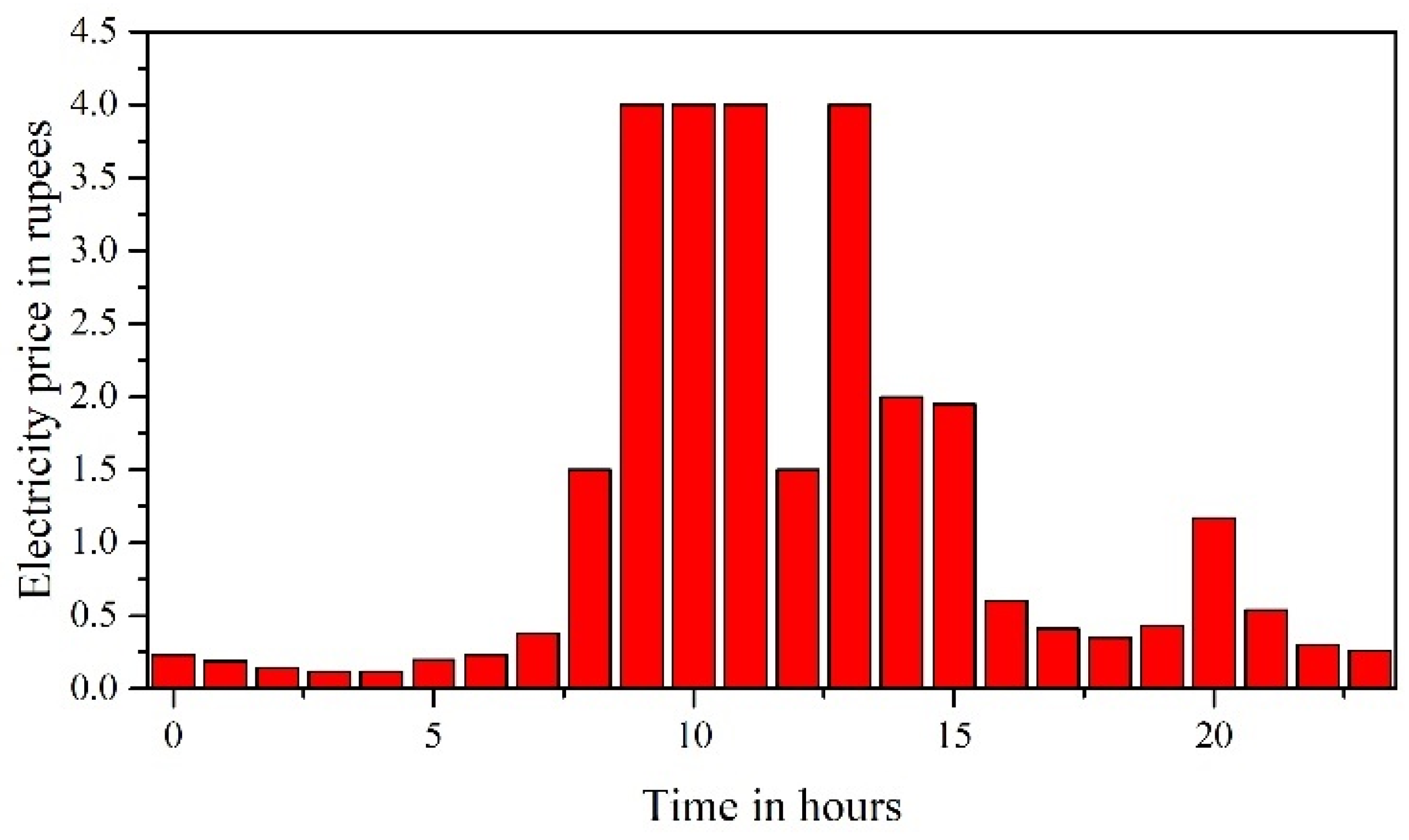
| Utility | Refer Figure 7 | −30 | 30 | ||
| Methodology | IEEE-18 Bus System | IEEE-33 Bus System | ||
|---|---|---|---|---|
| Total Cost in Rupees | Computational Time in Seconds | Total Cost in Rupees | Computational Time in Seconds | |
| GD optimization | 1661.7 | 0.483 | 12,350 | 1.23 |
| GJO optimization | 1660.8 | 0.480 | 12,332 | 1.08 |
| BB optimization | 1636.7 | 0.430 | 12,448 | 1.07 |
| Interior point optimization | 1679.4 | 0.531 | 12,412 | 1.12 |
| Proposed method | 1612 | 0.483 | 12,017 | 1.02 |
Disclaimer/Publisher’s Note: The statements, opinions and data contained in all publications are solely those of the individual author(s) and contributor(s) and not of MDPI and/or the editor(s). MDPI and/or the editor(s) disclaim responsibility for any injury to people or property resulting from any ideas, methods, instructions or products referred to in the content. |
© 2025 by the authors. Licensee MDPI, Basel, Switzerland. This article is an open access article distributed under the terms and conditions of the Creative Commons Attribution (CC BY) license (https://creativecommons.org/licenses/by/4.0/).
Share and Cite
Nandigam, S.H.; Pothireddy, K.M.R.; Rao, K.N.; Salkuti, S.R. Hybrid Adaptive Sheep Flock Optimization and Gradient Descent Optimization for Energy Management in a Grid-Connected Microgrid. Designs 2025, 9, 63. https://doi.org/10.3390/designs9030063
Nandigam SH, Pothireddy KMR, Rao KN, Salkuti SR. Hybrid Adaptive Sheep Flock Optimization and Gradient Descent Optimization for Energy Management in a Grid-Connected Microgrid. Designs. 2025; 9(3):63. https://doi.org/10.3390/designs9030063
Chicago/Turabian StyleNandigam, Sri Harish, Krishna Mohan Reddy Pothireddy, K. Nageswara Rao, and Surender Reddy Salkuti. 2025. "Hybrid Adaptive Sheep Flock Optimization and Gradient Descent Optimization for Energy Management in a Grid-Connected Microgrid" Designs 9, no. 3: 63. https://doi.org/10.3390/designs9030063
APA StyleNandigam, S. H., Pothireddy, K. M. R., Rao, K. N., & Salkuti, S. R. (2025). Hybrid Adaptive Sheep Flock Optimization and Gradient Descent Optimization for Energy Management in a Grid-Connected Microgrid. Designs, 9(3), 63. https://doi.org/10.3390/designs9030063