
Optimizing Beam Stiffness and Beam Modal Response with Variable Spacing and Extrusion (VaSE)

Abstract
1. Introduction
2. Materials and Methods
2.1. Methodology Behind the VaSE Algorithm
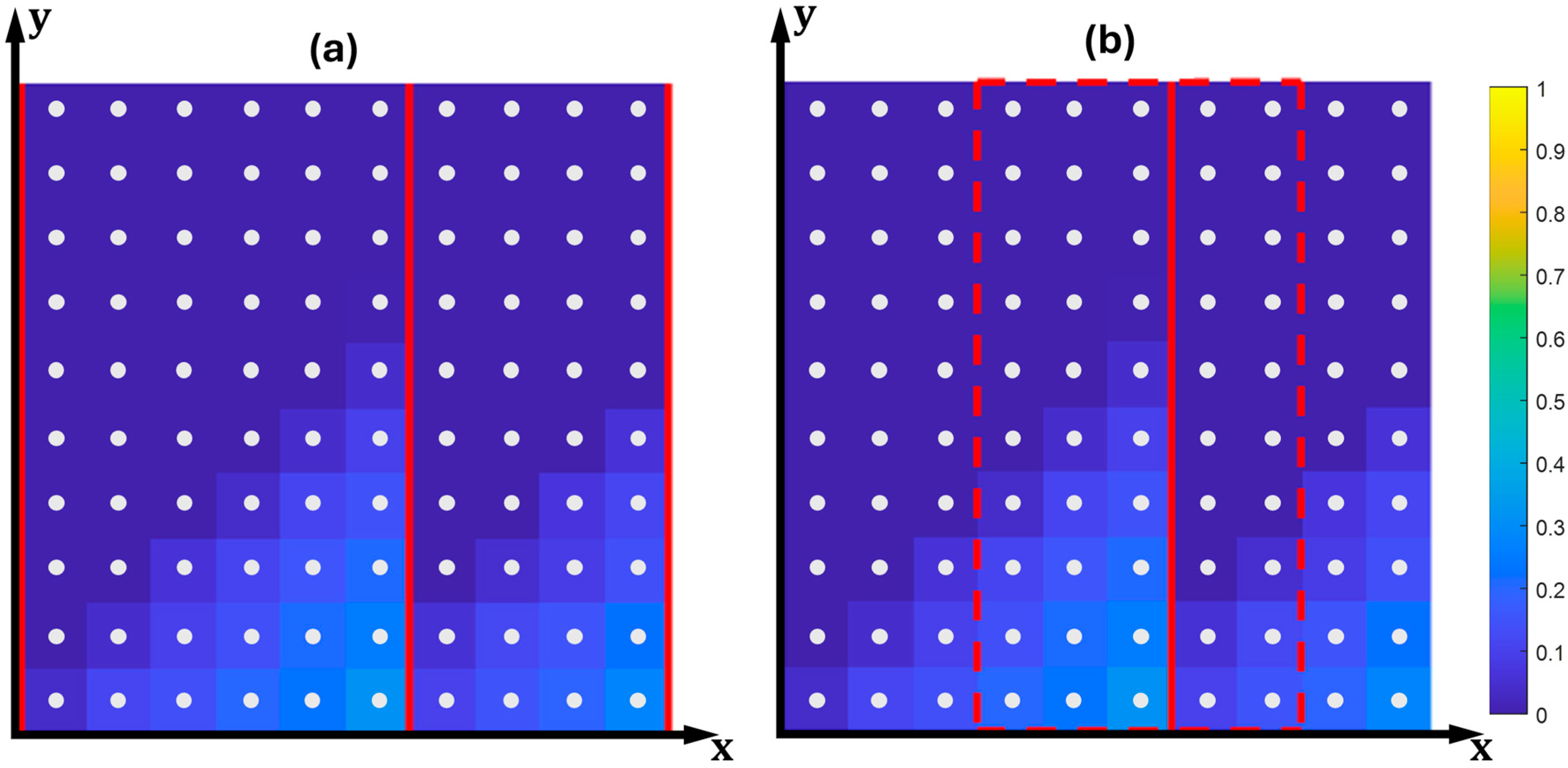
2.1.1. Creating a Toolpath to Obtain the Variable Line Spacing (VLS)
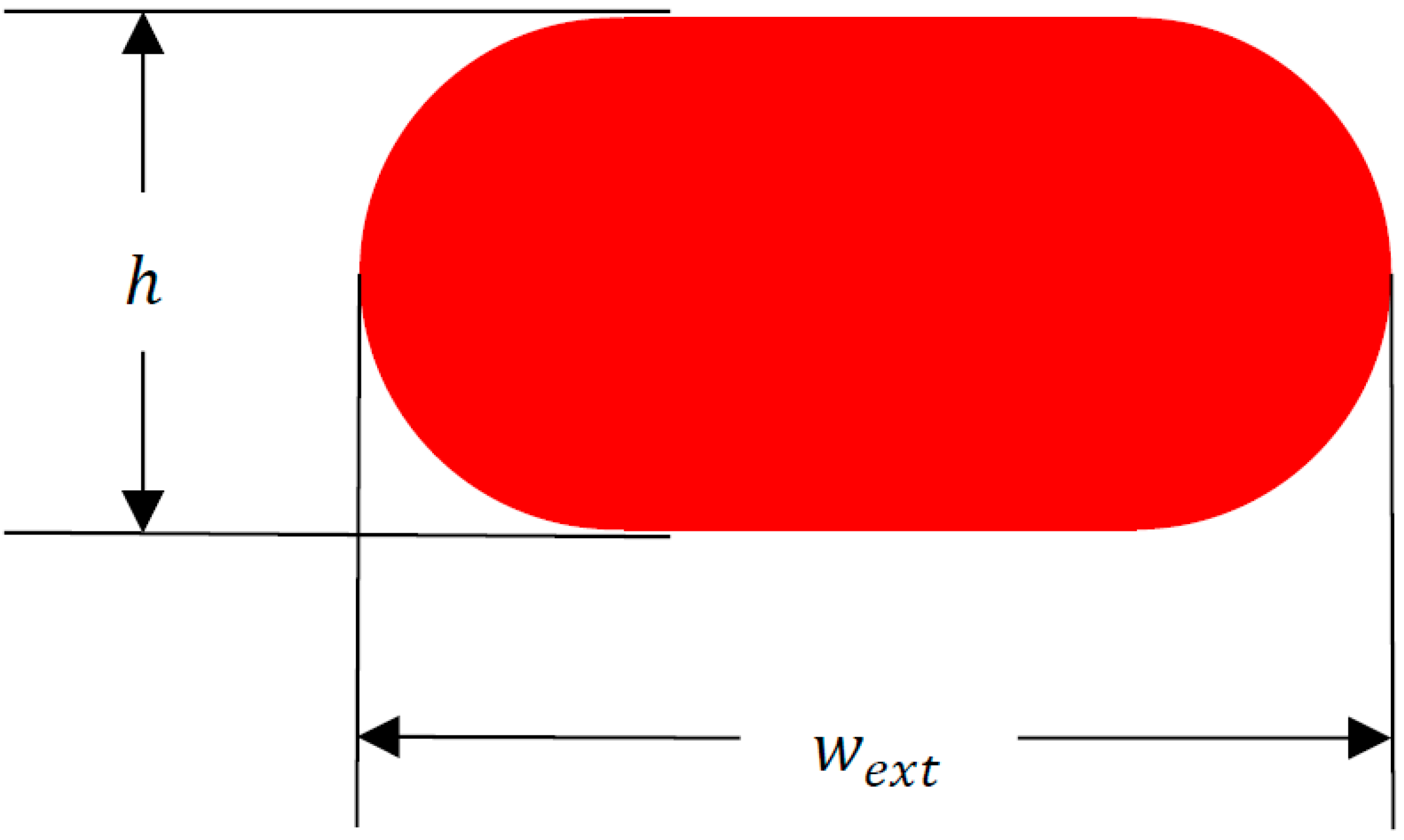
2.1.2. Determining the Variable Extrusion Width (VEW)
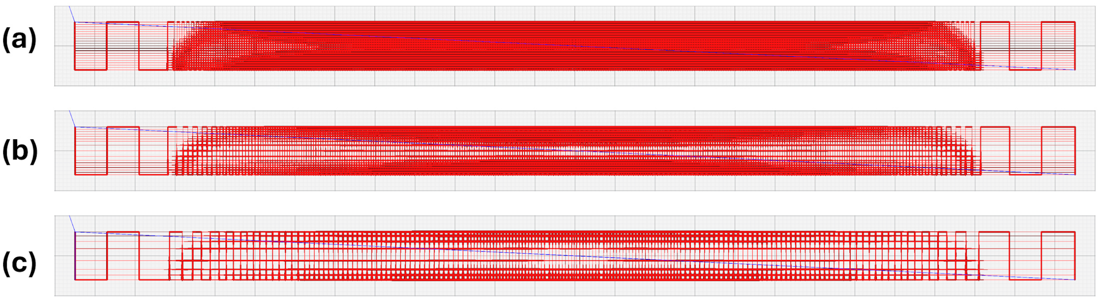
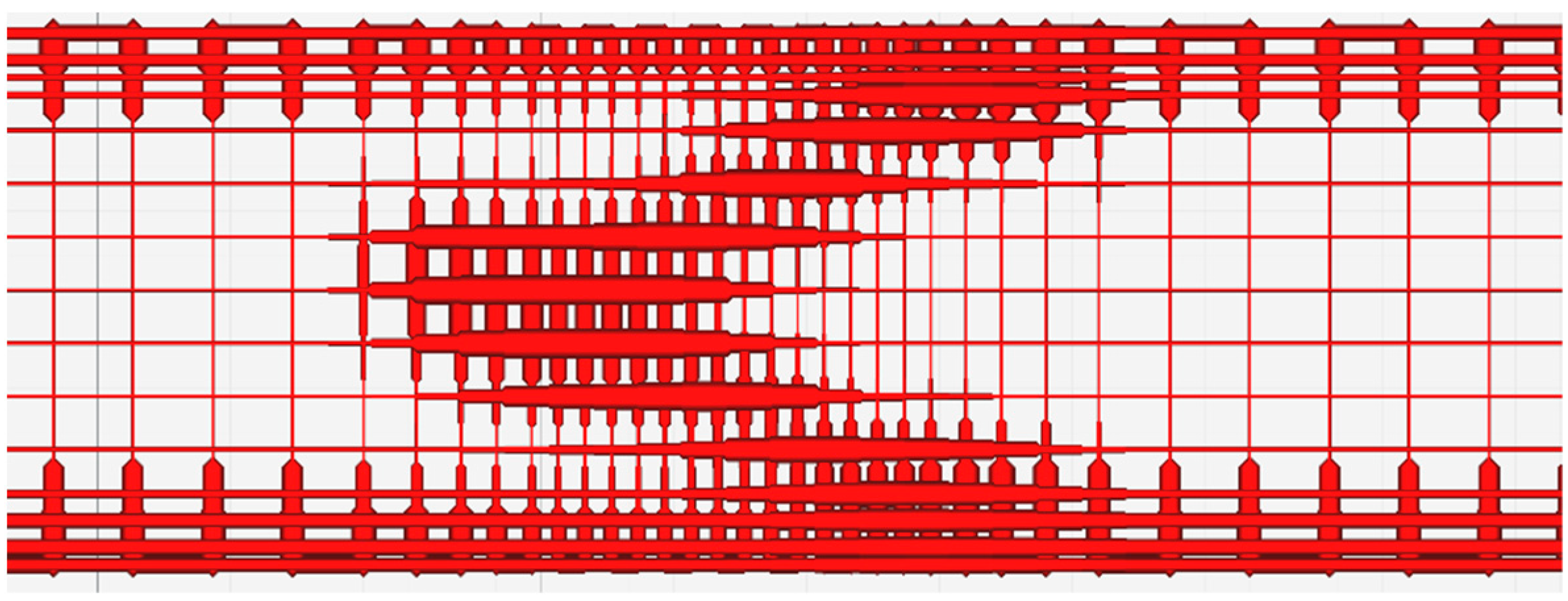
2.1.3. Piecing Together the Variable Line Spacing (VLS) and Variable Extrusion Width (VEW) to Create Usable Machine Parameters Commands for an ME Printer
| Algorithm 1 Generation of Machine Parameters |
|
3. Optimizing Beam Stiffness with the VaSE Algorithm
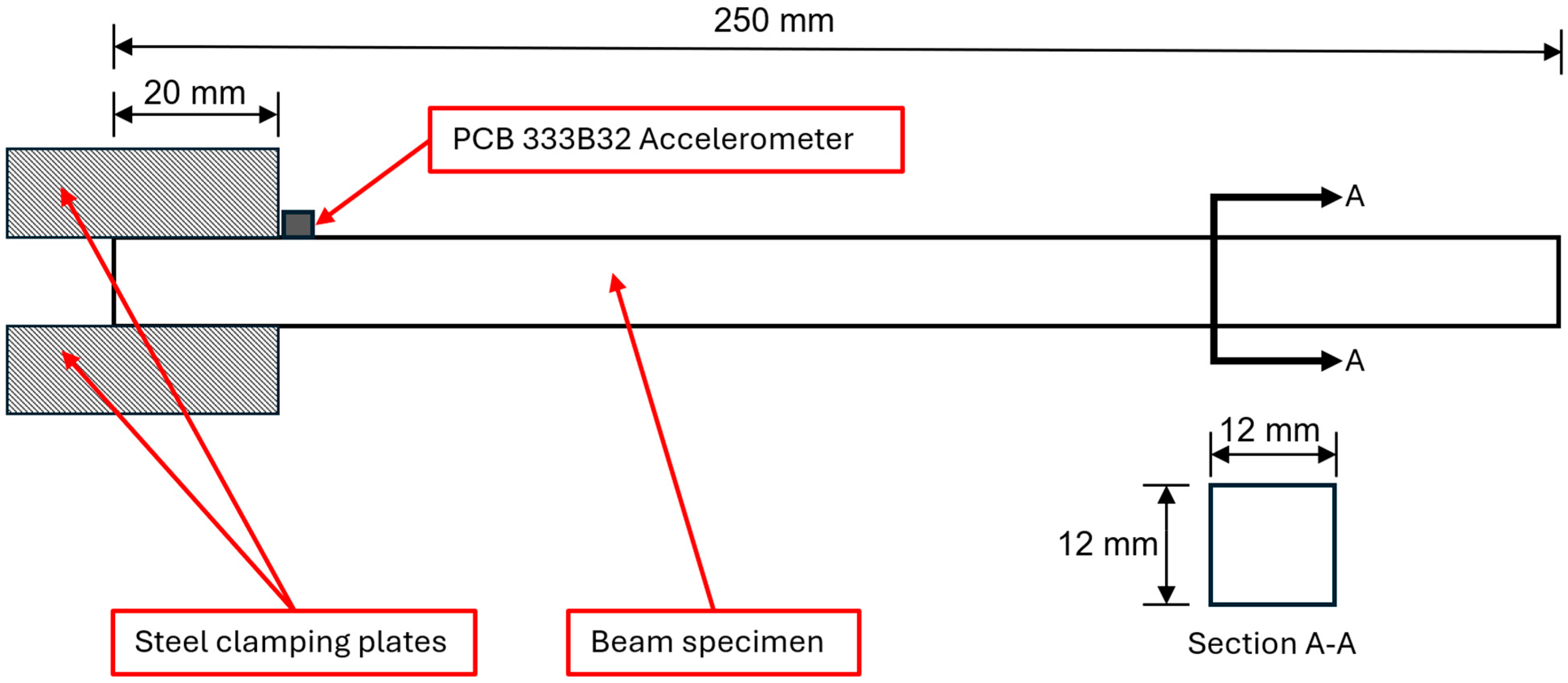
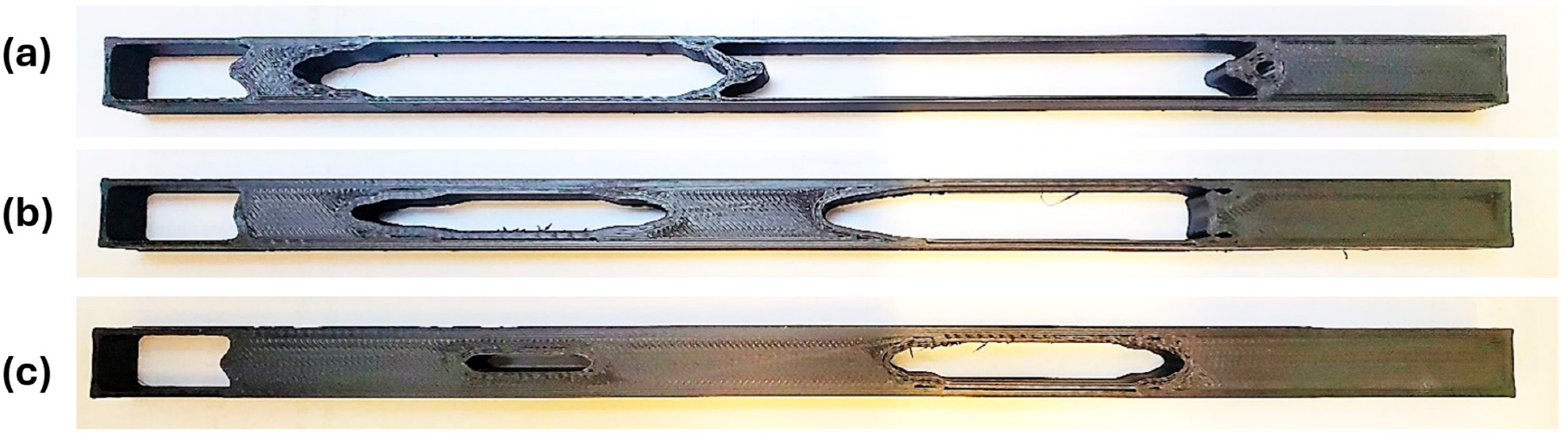
4. Optimizing Beam Modal Response Utilizing the VaSE Algorithm
5. Results and Discussion
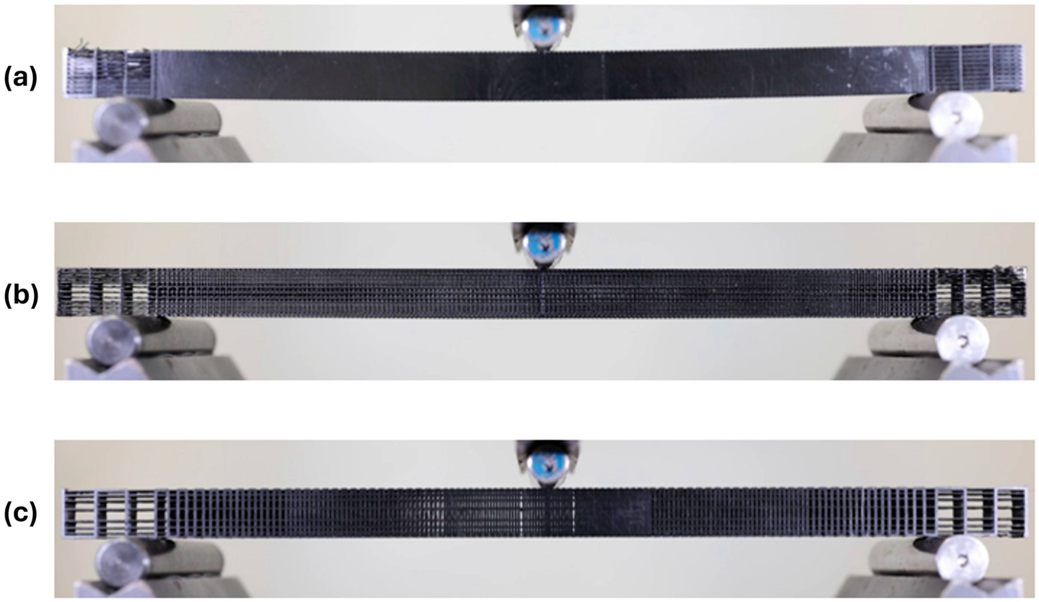
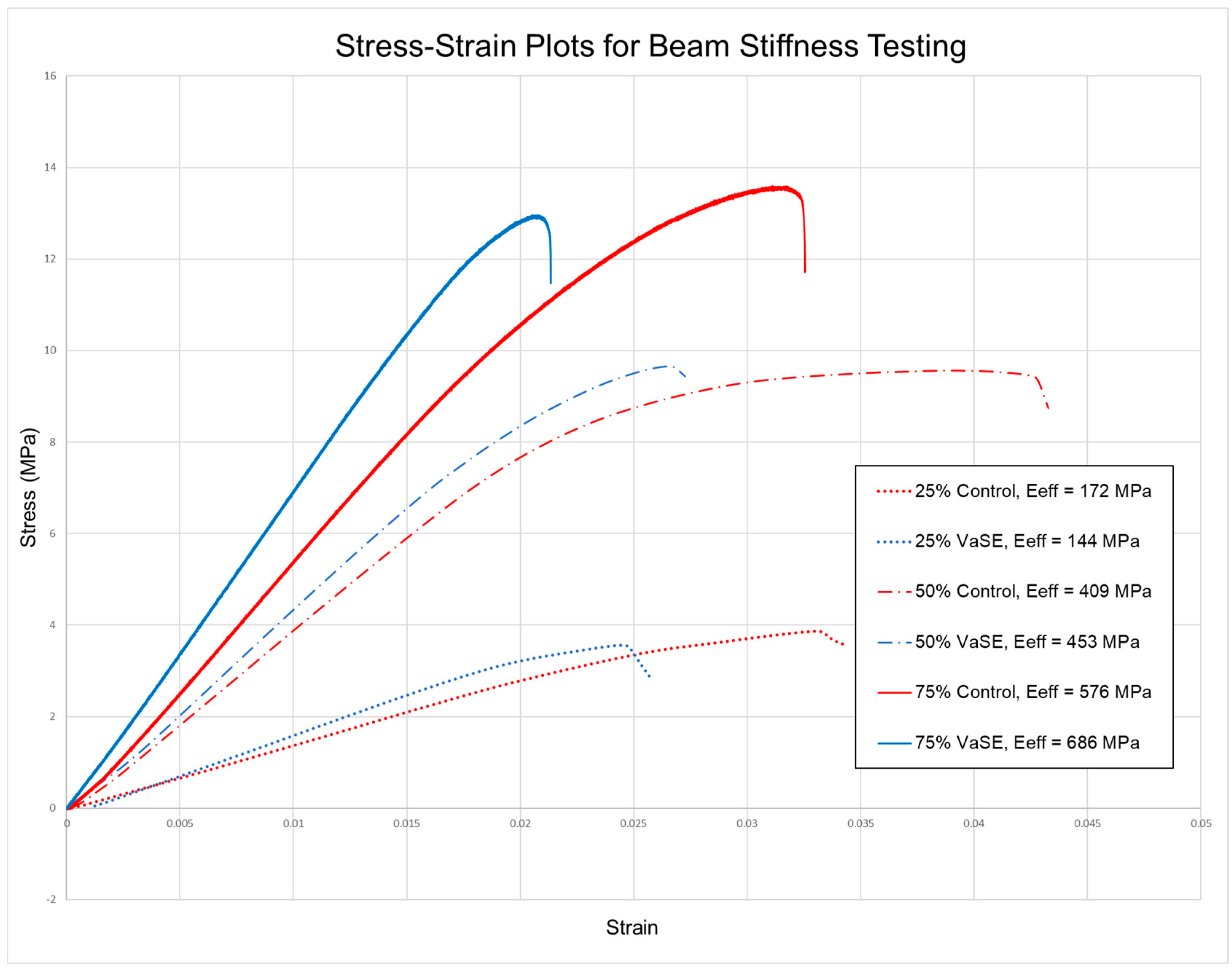
5.1. Beam Stiffness
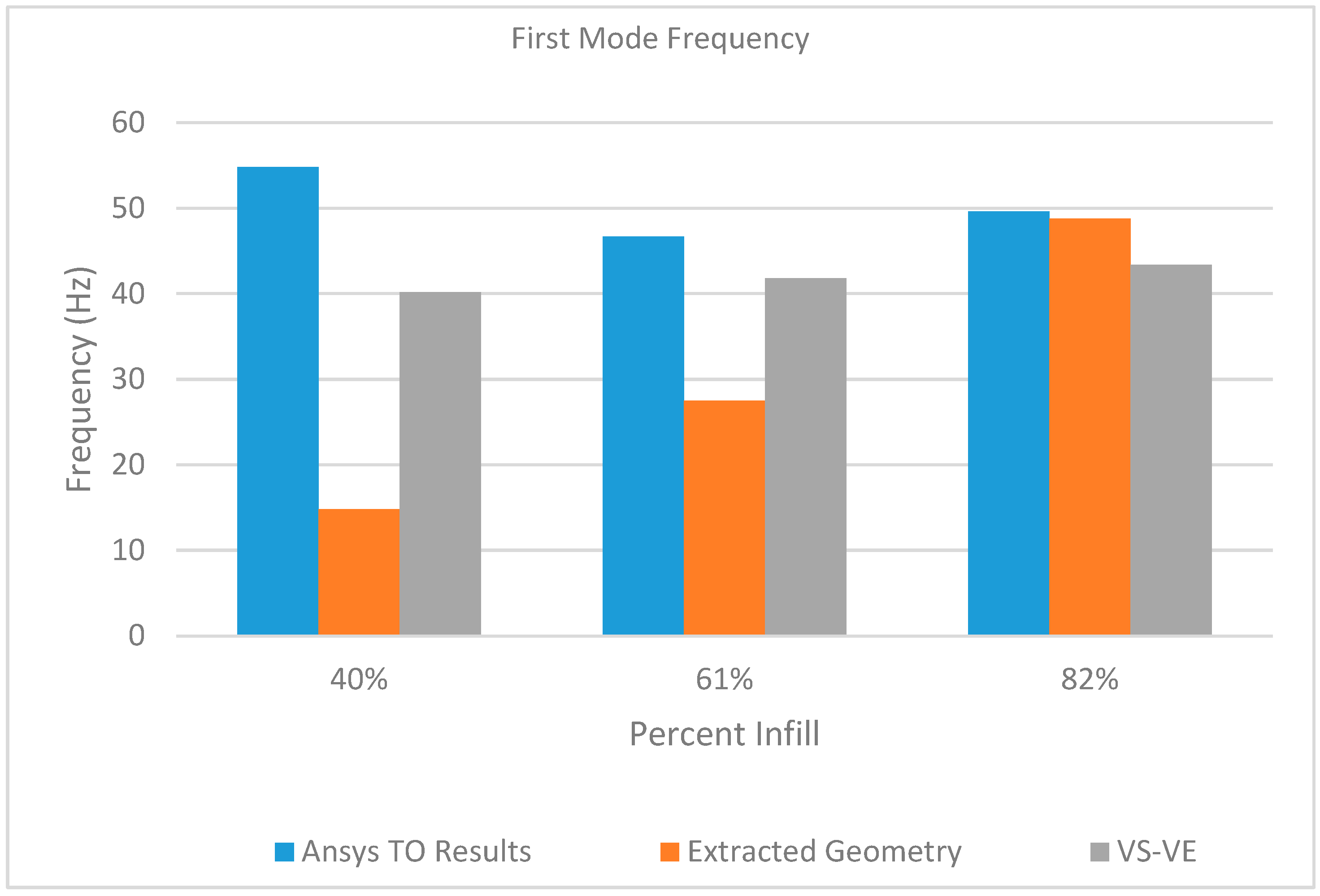
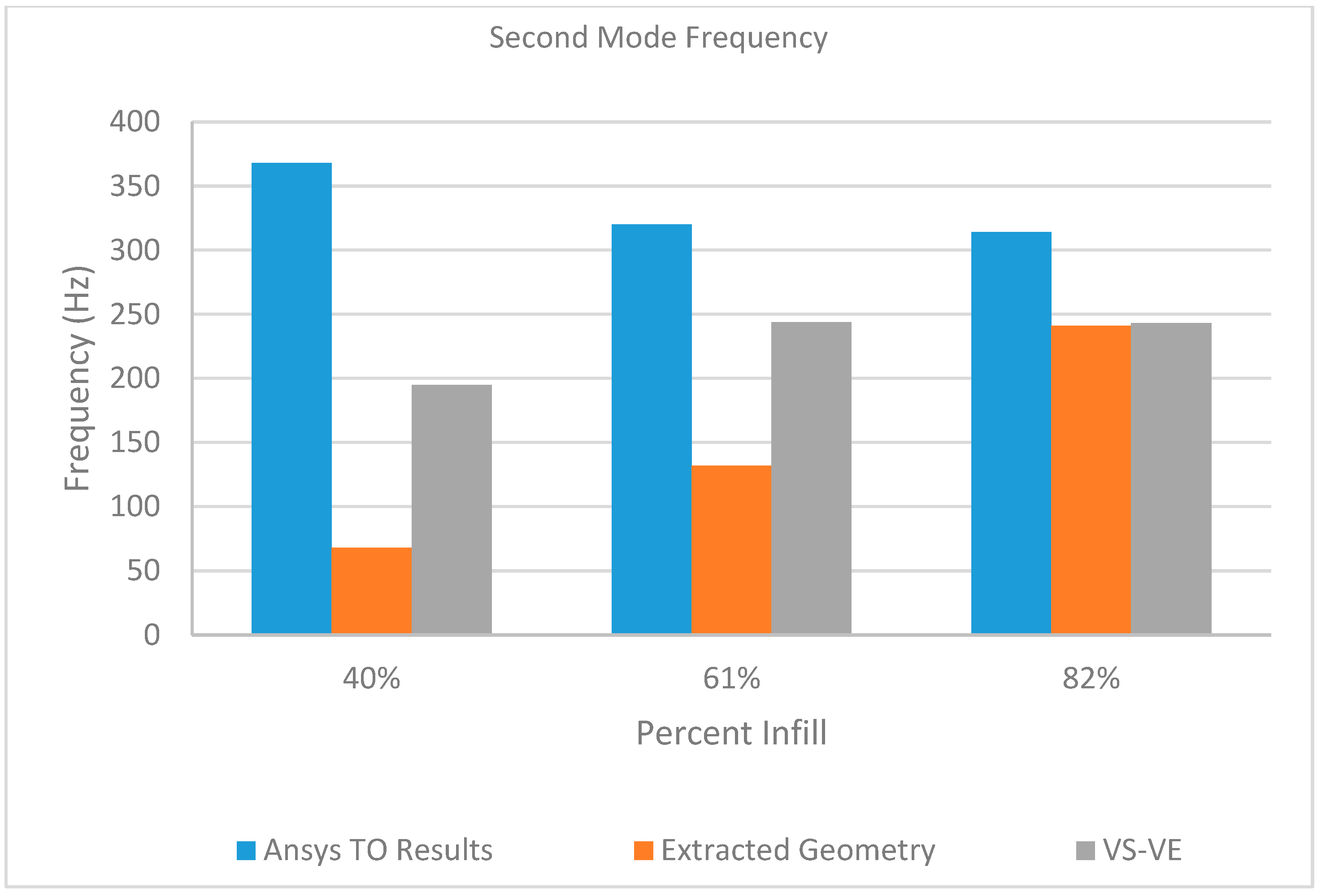
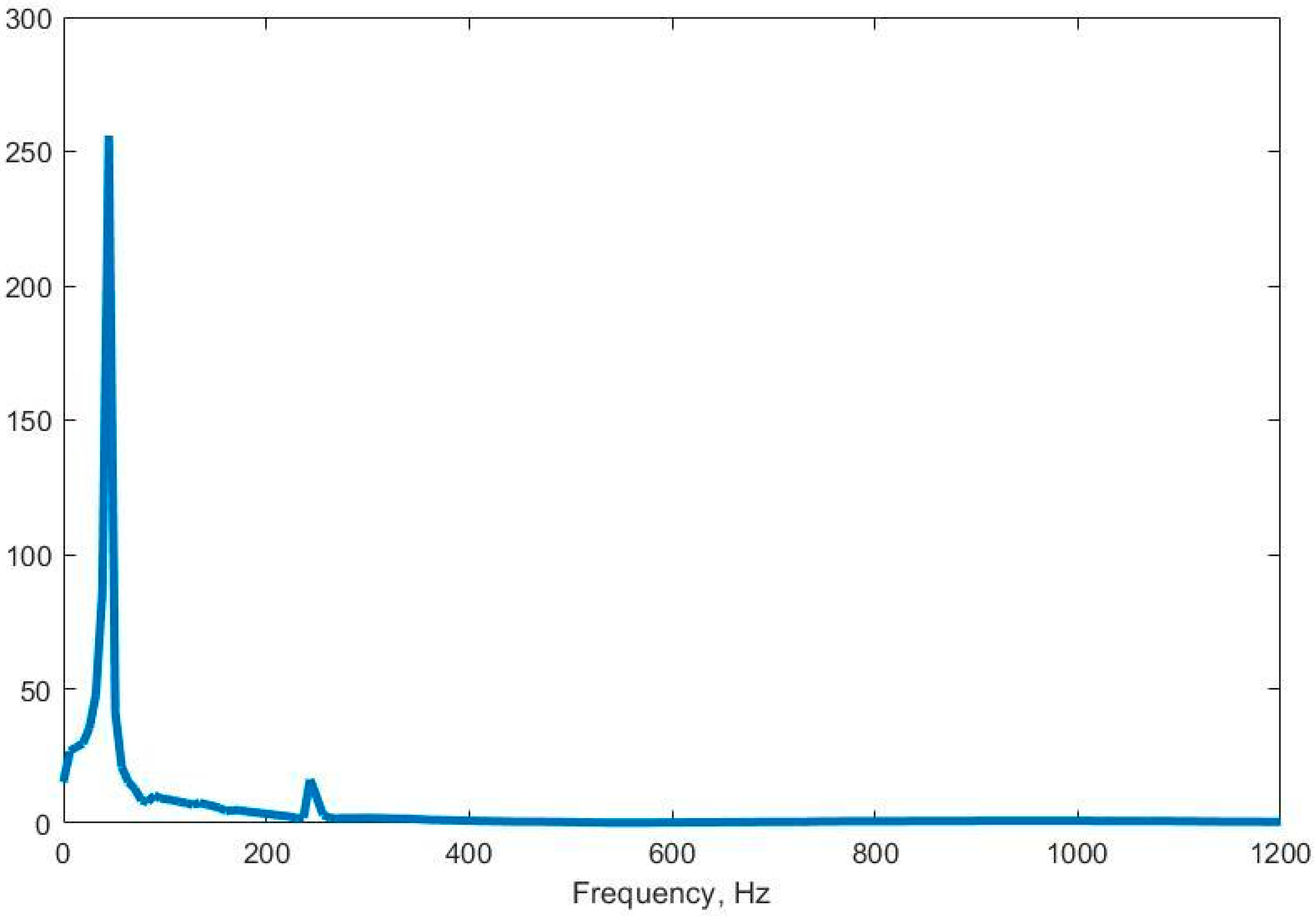
5.2. Modal Response
6. Conclusions
Author Contributions
Funding
Data Availability Statement
Conflicts of Interest
References
- Gibson, I.; Rosen, D.; Stucker, B.; Khorasani, M. Additive Manufacturing Technologies; Springer International Publishing: Cham, Switzerland, 2021. [Google Scholar] [CrossRef]
- Bacciaglia, A.; Ceruti, A.; Liverani, A. Additive Manufacturing Challenges and Future Developments in the Next Ten Years. In Design Tools and Methods in Industrial Engineering; Rizzi, C., Andrisano, A.O., Leali, F., Gherardini, F., Pini, F., Vergnano, A., Eds.; Springer International Publishing: Cham, Switzerland, 2020; pp. 891–902. [Google Scholar] [CrossRef]
- Dudescu, C.; Racz, L. Effects of Raster Orientation, Infill Rate and Infill Pattern on the Mechanical Properties of 3D Printed Materials. ACTA Univ. Cibiniensis 2017, 69, 23–30. [Google Scholar] [CrossRef]
- Fernandez-Vicente, M.; Calle, W.; Ferrandiz, S.; Conejero, A. Effect of Infill Parameters on Tensile Mechanical Behavior in Desktop 3D Printing. 3D Print. Addit. Manuf. 2016, 3, 183–192. [Google Scholar] [CrossRef]
- Cuan-Urquizo, E.; Álvarez-Trejo, A.; Gil, A.R.; Tejada-Ortigoza, V.; Camposeco-Negrete, C.; Uribe-Lam, E.; Treviño-Quintanilla, C.D. Effective Stiffness of Fused Deposition Modeling Infill Lattice Patterns Made of PLA-Wood Material. Polymers 2022, 14, 337. [Google Scholar] [CrossRef]
- Goh, G.D.; Yap, Y.L.; Tan, H.K.J.; Sing, S.L.; Goh, G.L.; Yeong, W.Y. Process–Structure–Properties in Polymer Additive Manufacturing via Material Extrusion: A Review. Crit. Rev. Solid State Mater. Sci. 2020, 45, 113–133. [Google Scholar] [CrossRef]
- Panesar, A.; Abdi, M.; Hickman, D.; Ashcroft, I. Strategies for functionally graded lattice structures derived using topology optimisation for Additive Manufacturing. Addit. Manuf. 2018, 19, 81–94. [Google Scholar] [CrossRef]
- Bendsøe, M.P.; Kikuchi, N. Generating optimal topologies in structural design using a homogenization method. Comput. Methods Appl. Mech. Eng. 1988, 71, 197–224. [Google Scholar] [CrossRef]
- Sigmund, O.; Maute, K. Topology optimization approaches: A comparative review. Struct. Multidiscip. Optim. 2013, 48, 1031–1055. [Google Scholar] [CrossRef]
- Pasko, A.; Fryazinov, O.; Vilbrandt, T.; Fayolle, P.-A.; Adzhiev, V. Procedural function-based modelling of volumetric microstructures. Graph. Models 2011, 73, 165–181. [Google Scholar] [CrossRef]
- Li, D.; Dai, N.; Jiang, X.; Shen, Z.; Chen, X. Density Aware Internal Supporting Structure Modeling of 3D Printed Objects. In Proceedings of the 2015 International Conference on Virtual Reality and Visualization (ICVRV), Xiamen, China, 17–18 October 2015; pp. 209–215. [Google Scholar] [CrossRef]
- Fryazinov, O.; Vilbrandt, T.; Pasko, A. Multi-Scale Space-Variant FRep Cellular Structures. Comput. Aided Des. 2013, 45, 26–34. [Google Scholar] [CrossRef]
- Xie, R.; Ulven, C.; Khoda, B. Design and Manufacturing of Variable Stiffness Mattress. Procedia Manuf. 2018, 26, 132–139. [Google Scholar] [CrossRef]
- Karamooz Ravari, M.R.; Kadkhodaei, M.; Badrossamay, M.; Rezaei, R. Numerical Investigation on Mechanical Properties of Cellular Lattice Structures Fabricated by Fused Deposition Modeling. Int. J. Mech. Sci. 2014, 88, 154–161. [Google Scholar] [CrossRef]
- Maskery, I.; Aremu, A.O.; Parry, L.; Wildman, R.D.; Tuck, C.J.; Ashcroft, I.A. Effective design and simulation of surface-based lattice structures featuring volume fraction and cell type grading. Mater. Des. 2018, 155, 220–232. [Google Scholar] [CrossRef]
- Yi, B.; Zhou, Y.; Yoon, G.H.; Saitou, K. Topology optimization of functionally-graded lattice structures with buckling constraints. Comput. Methods Appl. Mech. Eng. 2019, 354, 593–619. [Google Scholar] [CrossRef]
- Yamanaka, D.; Suzuki, H.; Ohtake, Y. Density aware shape modeling to control mass properties of 3D printed objects. In Proceedings of the SIGGRAPH Asia 2014 Technical Briefs, Shenzhen, China, 3–6 December 2014; pp. 1–4. [Google Scholar] [CrossRef]
- Aremu, A.O.; Brennan-Craddock, J.; Panesar, A.; Ashcroft, I.; Hague, R.; Wildman, R.; Tuck, C. A voxel-based method of constructing and skinning conformal and functionally graded lattice structures suitable for additive manufacturing. Addit. Manuf. 2017, 13, 1–13. [Google Scholar] [CrossRef]
- Brackett, D.J.; Ashcroft, I.A.; Wildman, R.D.; Hague, R.J.M. An Error Diffusion Based Method to Generate Functionally Graded Cellular Structures. Comput. Struct. 2014, 138, 102–111. [Google Scholar] [CrossRef]
- Cheng, L.; Bai, J.; To, A.C. Functionally Graded Lattice Structure Topology Optimization for the Design of Additive Manufactured Components with Stress Constraints. Comput. Methods Appl. Mech. Eng. 2019, 344, 334–359. [Google Scholar] [CrossRef]
- Yao, Y.; Cheng, L.; Li, Z. A comparative review of multi-axis 3D printing. J. Manuf. Process. 2024, 120, 1002–1022. [Google Scholar] [CrossRef]
- Grigolato, L.; Rosso, S.; Meneghello, R.; Concheri, G.; Savio, G. Design and manufacturing of graded density components by material extrusion technologies. Addit. Manuf. 2022, 57, 102950. [Google Scholar] [CrossRef]
- Murphy, P.N.; Khoda, B. Application of a Continuous Variable Density Infill: Manipulating Center of Gravity. In Proceedings of the ASME 2023 International Design Engineering Technical Conferences and Computers and Information in Engineering Conference, Boston, MA, USA, 20–23 August 2023. [Google Scholar] [CrossRef]
- Murphy, P. A Novel Functionally Graded Infill Method for Realizing Topology Optimization for Additive Manufacturing. Master’s Thesis, University of Maine, Orono, ME, USA, 2024. Available online: https://digitalcommons.library.umaine.edu/etd/3992 (accessed on 1 January 2025).
- Ahsan, A.; Xie, R.; Khoda, B. Heterogeneous topology design and voxel-based bio-printing. RPJ 2018, 24, 1142–1154. [Google Scholar] [CrossRef]
- Sigmund, O. A 99 line topology optimization code written in Matlab. Struct. Multidiscip. Optim. 2001, 21, 120–127. [Google Scholar] [CrossRef]
- Özsoy, K.; Erçetin, A.; Çevik, Z.A. Comparison of Mechanical Properties of PLA and ABS Based Structures Produced by Fused Deposition Modelling Additive Manufacturing. Eur. J. Sci. Technol. 2021, 802–809. [Google Scholar] [CrossRef]
- Wu, P.; Ramani, K.S.; Okwudire, C.E. Accurate linear and nonlinear model-based feedforward deposition control for material extrusion additive manufacturing. Addit. Manuf. 2021, 48, 102389. [Google Scholar] [CrossRef]
- Chesser, P.; Post, B.; Roschli, A.; Carnal, C.; Lind, R.; Borish, M.; Love, L. Extrusion control for high quality printing on Big Area Additive Manufacturing (BAAM) systems. Addit. Manuf. 2019, 28, 445–455. [Google Scholar] [CrossRef]


Disclaimer/Publisher’s Note: The statements, opinions and data contained in all publications are solely those of the individual author(s) and contributor(s) and not of MDPI and/or the editor(s). MDPI and/or the editor(s) disclaim responsibility for any injury to people or property resulting from any ideas, methods, instructions or products referred to in the content. |
© 2025 by the authors. Licensee MDPI, Basel, Switzerland. This article is an open access article distributed under the terms and conditions of the Creative Commons Attribution (CC BY) license (https://creativecommons.org/licenses/by/4.0/).
Share and Cite
Murphy, P.N.; Vittum, R.A., III; Khoda, B. Optimizing Beam Stiffness and Beam Modal Response with Variable Spacing and Extrusion (VaSE). Designs 2025, 9, 64. https://doi.org/10.3390/designs9030064
Murphy PN, Vittum RA III, Khoda B. Optimizing Beam Stiffness and Beam Modal Response with Variable Spacing and Extrusion (VaSE). Designs. 2025; 9(3):64. https://doi.org/10.3390/designs9030064
Chicago/Turabian StyleMurphy, Patrick N., Richard A. Vittum, III, and Bashir Khoda. 2025. "Optimizing Beam Stiffness and Beam Modal Response with Variable Spacing and Extrusion (VaSE)" Designs 9, no. 3: 64. https://doi.org/10.3390/designs9030064
APA StyleMurphy, P. N., Vittum, R. A., III, & Khoda, B. (2025). Optimizing Beam Stiffness and Beam Modal Response with Variable Spacing and Extrusion (VaSE). Designs, 9(3), 64. https://doi.org/10.3390/designs9030064