On the Design of Smooth Curvature Tunable Paths for Safe Motion of Autonomous Vehicles

Abstract

Navigation is an essential ability for autonomous systems, and efficient motion planning for mobile robots is a central topic for autonomous vehicle design and service robotics. Most path-planning algorithms produce reference paths with sharp or discontinuous turns, inducing several drawbacks during mission execution, such as unexpected inertial stress and strain on the mechanical structure, passenger discomfort, and unsafe and unpredictable deviation of the real trajectory with respect to the reference planned one. Oppositely, smooth and feasible trajectories are often desired in real-time navigation for nonholonomic mobile robots where the surrounding environment can have a dynamic and complex shape with obstacles. In this paper, we propose a novel technique for the generation of smooth, collision-free, and near time-optimal paths for nonholonomic mobile robots. The proposed method exploits the features of a set of tunable bump functions, with the goal of pursuing smooth reference curves with tunable features (such as curvature, or jerk) yet seeking a reasonable length minimality, thus combining the advantages of the two most adopted techniques, namely Bezier interpolation and Dubins curves. After a thorough description of the analytical methods, the paper is primarily concerned with the design and tuning methods of the path-planning algorithm. Both a graphical method and numerical investigations and examples are performed to fully exploit the algorithm potentialities and to show the efficiency of the proposed strategy.

1. Introduction

Recent advances of modern technologies make tomorrow’s world a place where humans and machines are more and more integrated in society. The topic of designing autonomous driving vehicles is a powerful example of integrated technologies and sophisticated algorithms with humans.

One key ability to reach autonomy for a mobile device is decision-making in planning its motion in the environment, namely its ability to find feasible paths in several diverse, dynamically varying environments, avoiding moving obstacles and minimizing the total travel length for achieving minimal travel time or energy consumption purposes. For this reason, the challenging problem of safe and autonomous navigation has surged as a central topic in the wide area of robotics and autonomous systems [1].

Navigation is a fundamental ability for autonomous systems. However, most path planning algorithms generate a reference path with many sharp or discontinuous turns, inducing several drawbacks during mission execution, such as unexpected inertial stress and strain on the mechanical structure, passenger discomfort, and unsafe and unpredictable deviation of the actual trajectory. Oppositely, smooth and feasible trajectories are often desired or requested for an overall satisfactory behavior of the feedback system; most convergence results assume indeed that the reference signal is smooth [2,3].

Among the most studied models representing the vehicle motion, the ‘Dubins vehicle’ [1] models a basic yet effective kinematic behavior. In essence, it describes the motion of a point in the plane having fixed forward speed and limited steering angle. Its popularity is related to its simplicity and that it is well suited to describe the movement of any vehicle whenever it is not required to make hard braking, slowdown or stop operations, which are often undesired or impossible in most applications.

The adoption of a Dubins model for path planning leads to navigation solutions in many diverse fields and in air, ground and marine applications. In the relevant field of aerial applications, the judicious management of tasks such as surveillance, reconnaissance, and delivery operations require careful path planning [4]. Aircraft, especially those with limited maneuverability, may encounter a precise way point crossing during specific tasks of flight mission [5], such as air-to-air refueling or navigating through airspace restrictions. In such scenarios, a safe, precise and efficient path planning is of paramount importance. Analogous considerations hold for marine and underwater applications, and hence the Dubins vehicle is often the chosen model for path planning [6].

However, despite the popularity and ubiquity of Dubins solutions in a variety of path-planning algorithms, there are several drawbacks that make this choice critical, and in the last decades there have been more and more attempts by researchers to overcome them through more sophisticated algorithms.

One peculiarity of Dubins paths which can produce serious drawbacks in practical applications is that length-optimal solutions naturally have non-differentiable curvature. Indeed, a characteristic feature of these paths is that the curvature switches between three values, namely zero and maximum left and right turn, thus the corresponding curvature profile has a rectangular shape.

The temporal discontinuity of the curvature function is usually a negative feature for the performance of a tracking control system, which in general requires a high degree of smoothness of the reference to guarantee good tracking performance (see e.g., [2,3]). What happens in practice when discontinuous reference signals are assigned is that the tracking error shows an abrupt deviation at the discontinuity time instants that converges to zero for the stabilizing action of the control system. It is worth remarking that, in all the application examples described above and many others, the occurrence of jumps in the tracking error is negative in terms of safety (since the real trajectory deviates from the expected one) and mission goal achievement (several discontinuity time instants may produce a deviation which is not recoverable during the mission execution).

For all these reasons, in the last decades, the scientific community has tried to extend the classical path planning based on the Dubins model in several different directions, with the goal of ensuring the continuity and differentiability of the reference path, as we briefly describe in the following.

1.1. Literature Review

One first attempt to generalize the Dubins vehicle model to exclude discontinuities in the curvature shape is to extend the state of configurations including the curvature rate. This model was introduced in the seminal paper [7], and widely studied later by several authors. In this framework, clothoid curves emerge as extremal curves of length-optimal problems, but solving the optimal control problem shows that an optimal trajectory containing one linear segment must have an infinite concatenation of clothoids [7], so that it is not convenient to adopt such mathematical optimal solution in practice. Notwithstanding this negative result about optmality, clothoid-shape reference paths have been largely investigated [8]. A recent detailed paper on clothoid is [9]. In the recent paper [10], clothoid-shaped primitives are integrated with a two-way D* for real-time navigation of nonholonomic mobile robots in dynamic and complex environments while avoiding obstacles.

However, there are several applications in which clothoid-shaped reference paths are not well suited, and there are several research activities trying to generalize the reference path shape to more general and smoother profiles.

In aerial and marine applications, vehicle propulsion and motion is based on the interaction with air or water, and the inertial drag of the vehicle body allows to track trajectories with slow curvature rate [11,12]. Motion control for these vehicles is therefore exceptionally hard, and highly smooth reference paths are often a primary choice [13].

More in detail, vehicle motion in marine or aerial applications is generated through fluidodynamical interactions, so that the tracking error of a discontinuous reference signal is usually large, and it makes the vehicle susceptible to large deviation of the actual motion from the expected one. This phenomenon can be a serious drawback in terms of safety, since the avoidance of obstacles is guaranteed by the attainment of the reference path, so that large deviations can lead to unpredictable collisions. Moreover, they induce a huge transient phase that is susceptible to unexpected oscillations and possible loss of stability. As for example, considering marine applications, in the paper [2] a dynamic control law making the system converge to the origin at an exponential rate is proposed, under the assumption that a pre-defined twice differentiable reference trajectory is set. In the framework of aerial applications, in the paper [3] the tackled trajectory tracking problem and the convergence results are achieved under the assumption that a sufficiently smooth desired trajectory with bounded derivatives is provided. Under this hypothesis, a controller is designed such that all the closed-loop signals are bounded and the trajectory tracking error converges to an arbitrarily small neighborhood of the origin.

For these reasons, most path-planning algorithms in this framework are designed through Bezier curves [14,15]. Their advantages are generality, conceptual simplicity, and high continuity. However, collision, via-point crossing and curvature-constraint checking must usually be done numerically in the case of such primitives, which leads to significant computational cost. We discuss the main advantages and drawbacks of using Bezier curves in Section 2.2.

Finally, one different novel yet relevant application field pushing toward the use of path-planning algorithms producing smooth reference profiles is service robotics. Indeed, more and more often robotics is adopted for human transport and assistance, ranging from urban mobility to personal assistance through automated wheelchairs. In most of the applications within this framework, robots interact with fragile humans, or they may carry delicate or dangerous items. Reference paths with discontinuous curvature are inconvenient, as their tracking would produce discomfort and possible accidents. Wheeled mobile robots following a path with continuous curvature may also benefit on wheels slippage reduction and low odometry errors, since transitions are softer with constant curvature rates. It is worth remarking that slippage phenomena are detrimental to precise control, and they can be compensated adopting sophisticated ad hoc algorithms [16]. On the contrary, smooth trajectories are often desired for a pleasant and safe mission execution. In all the applications where human users are involved, comfort is adopted as a criterion for design. In [17] propose a tunable trajectory planner generating G3 curves for road vehicles. The path-planning algorithm in [18] produces smooth profiles for a better tracking performance of the vehicle.

1.2. Paper Contribution

Considering all the above discussion, the goal of this paper is to derive an algorithm for the construction of reference paths having smooth curvature along the way, with the opportunity to set the curvature bound together with the first and second derivatives, and ensuring the via-point crossing. The paper [13] is inspired by analogous considerations, and the proposed solution allows building smooth reference trajectories. However, the solution proposed in this paper significantly differs from the above solution in terms of presence of parameter values that allow a tuning of the shape of the curvature function to meet possible constraints on the curvature up to the second derivative. Also, the reference path construction follows a different logic.

One main purpose of the proposed research activity is the generation of reference trajectories that allow safe and comfortable behavior to a vehicle having the ability to track them. The two terms, namely safe and comfortable, related to different goals. The former refers to a vehicle traveling free from accidents and undesired deviations, and it is strictly related to the feasibility of a reference trajectory by the vehicle. The latter refers to reference trajectories whose tracking does not generate lateral accelerations and impulsive inertial forces [19]. Considering all these diverse facets of control goals, we seek a reference curvature profile with tunable bounds on the maximum curvature together with first and second derivatives, considering that such bounds have been set as a reasonable trade-off between all the above features.

2. Problem Framework

In this Section, we fully describe and state the problem tackled in this paper as an advancement in the topic of local path-planning algorithms. We start with the genuine description of the most relevant features of a path-planning algorithm, with focus on the applications described above. Then we describe the advantages and drawbacks of the two most adopted approaches, namely Bezier curves and Dubins paths, and finally we formally state the tackled problem.

2.1. Path Planning for Mobile Robots

Path planning algorithms are an essential part of a control system for a mobile device and autonomous vehicles [1]. It typically receives as inputs an a priori knowledge of the environment (e.g., maps), some knowledge provided by sensors (e.g., localization) and the desired goal to achieve (e.g., achieve a given pose in a remote location of the map), and it provides as output a reference trajectory to be tracked by the mobile device so to accomplish the assigned task [1]. To solve this problem, path-planning algorithms can be classified as global or local path planning algorithms. Global path-planning algorithms exploit pre-computed environmental data (e.g., maps) to compute the optimal path from start to destination before the mission execution, thus computing the most efficient route from start to goal. Traditional solving methods make use of graph search tools or optimization-based search approaches (e.g., particle swarm optimization, Ant Colony Optimization), while modern approaches take advantage of artificial intelligence methods (e.g., deep learning). Oppositely, local path-planning algorithms are concerned with the problem of connecting two positions exploiting real-time data from sensors to continuously update the path and distance to the target, while incorporating objectives for trajectory smoothness and minimal jerk. Most path-planning algorithms are usually organized in two stages, taking advantage of the features of each of the two approaches. One stage is focused on the selection of a set of convenient way points in the map and it is useful to build a rough route, the other stage being establishing the connections between the selected way points through convenient primitives or interpolating curves to build a viable path to be tracked by the device [1]. Besides the spatial profile of the reference path, the output of a path planner and one major goal of a navigation system is the generation of a guidance law for the vehicle, namely the temporal profile that should be impressed to the input of the vehicle in order to follow a reference path leading to goal achievement.

Overall, the path-planning algorithm is designed to consider some basic performances. The generated path must be safe, namely free from collisions with the environment. It must be feasible by the mobile device, so that it can be asymptotically tracked by a real robot through a suitable control system algorithm. It additionally must be reasonably short, namely having length minimality properties, which is a desired feature for several reasons, e.g., for fuel savings, which is important for an autonomous device to minimize the need for fuel. Finally, for recent applications, the algorithm must be sufficiently fast, namely the time needed for its execution should be negligible so that it can be run in real-time when the device moves in a dynamic environment, and it must eventually update the reference path due to perturbed conditions.

However, most path-planning algorithms produce reference paths made of straight lines connected through sharp turns [20]. Such paths are not a good choice for robot motion in many modern applications of practical interest, as we detail later in Section 2.2. The main reason is that a mobile device cannot make these sharp turns suddenly when moving at cruise speed, and it would be necessary to stop or slow down to track them. Alternatively, the tracking error shows deviations when discontinuity points occur.

Unfortunately, the former operational way to track the reference path, namely adjusting the cruise speed for tracking purposes, is not possible in most aerial or marine applications, or they turn out to be highly inconvenient for road or ground vehicles for inducing user discomfort or inertial accelerations that solicit undesired unmodeled dynamics which may perturb the system even to instability.

In the paper [21], continuous curvature reference paths are built to attain human comfort together with other goal achievement.

2.2. Smoothing Bezier Curves and Dubins Primitives

Before discussing the proposed approach in detail, in this Section we describe the advantages and drawbacks of the two main classical tools for generating reference paths which are mostly adopted as local solvers in the guidance algorithms for vehicles, namely the interpolation of two or more points using Bezier curves and Dubins primitives. The outcome of this investigation allows us to focus on the features that our algorithm must hold, while avoiding the main drawbacks associated to the use of traditional approaches.

One of the most popular methods to build reference paths is through the Bezier curve interpolation [22]. These parametric curves make use of ‘control points’ to define the shape of the generated curve. In essence, they exploit Bernstein polynomials as follows. For an assigned set of $n+1$ points ${\mathbf{P}}_0$, ${\mathbf{P}}_1$, …, ${\mathbf{P}}_n$ called control points, the interpolating Bézier curve is defined as:

$$\mathbf{p}\left(t\right)=\sum _{i=0}^n{B}_i^n\left(t\right){\mathbf{P}}_0,t\in [0,1],$$

(1)

where the blending functions $B_i^n\left(t\right)$ are the Bernstein polynomials equal to:

$$B_i^n\left(t\right)=\left({\displaystyle \genfrac{}{}{0pt}{}{n}{i}}\right){(1-t)}^{n-i}{t}^i,i\in \{0,1,\dots ,n\}.$$

(2)

Since their introduction nearly one century ago, their use has been intense in various topics, ranging from computer graphics and animation to robotics [22].

Bezier curves success is undoubtedly related to its ease of use, its smoothness properties, and its flexibility and ease of shape modeling through a tuning of the relative control points.

Unfortunately, both length optimality and bounded curvature properties of a path for vehicles like mobile robots cannot be obtained with analytical methods, but heuristic algorithms are adopted [23]. In this framework, the problem is usually translated into finding the optimal placement of control points or modifying curve parameters, often using heuristic methods to find the actual maximum curvature, which isn’t easily found in closed form.

Another drawback in the use of this method is the exact crossing of the via points, which cannot be directly guaranteed and requires specific attention [24].

2.3. Dubins Vehicle Model

We here briefly mathematically describe the widely adopted Dubins vehicle model, and we introduce the notation that we use along the paper.

The Dubins car model describes the kinematics of a mobile device moving forward at constant velocity with limited steering capability. Consider a particle in the $x-y$ plane moving according to the following kinematics:

$$\left\{\begin{array}{c}\dot{x}=cos\theta ,\hfill \\ \dot{y}=sin\theta ,\hfill \\ \dot{\theta }=k,\hfill \\ \left|\right|k\left|\right|\le \mathsf{\Omega };\hfill \end{array}\right.$$

(3)

where $\mathsf{\Omega }$ is a known constant. From a geometric perspective, Equation (3) describes a vehicle moving only forward at a constant speed equal to one and limited steering ability with a maximum turning radius ${\mathsf{\Omega }}^{-1}$. Equation (3) is referred to as the Dubins’ car model [1]. In this framework, a path is called feasible for a Dubins vehicle if it can be generated through (3), so that feasible curves are essentially those plane curves with curvature lower than $\mathsf{\Omega }$.

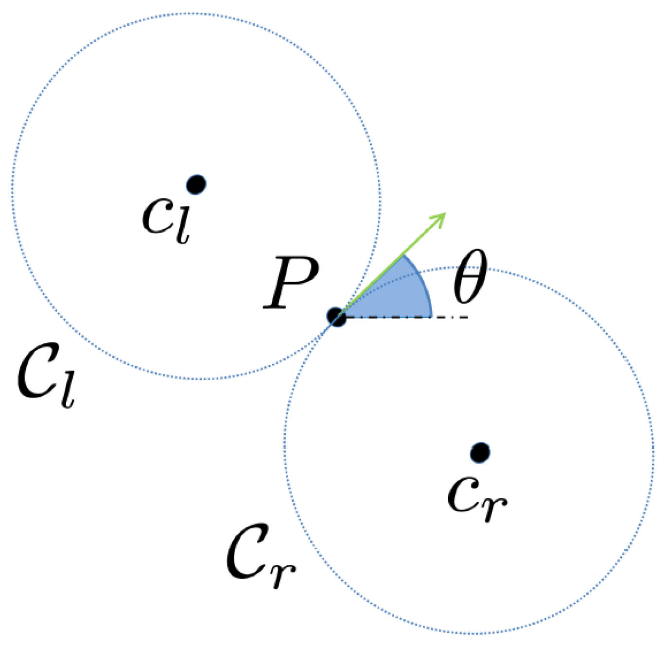
Consider Figure 1. Vector $\mathbf{q}=(\mathit{P},$ $\theta$) is called the pose or configuration of the vehicle described in (3), $\mathit{P}=(x,y)$ representing the position of the vehicle in the Euclidean plane, $\theta \in [0,2\pi )$ its orientation (see Figure 1. In this basic framework the angular speed u is assumed to be the control signal as input of the vehicle.

When dealing with Dubins vehicles, it is common to graphically draw two circles of radius ${\mathsf{\Omega }}^{-1}$ tangent to $\mathbf{q}$ in $\mathit{P}$ that we call resp. left circle and right circle, each corresponding to the sharpest turn.

The use of Equation (3) is popular in mobile robotics as it provides a simple yet effective kinematic model for a variety of mobile devices and vehicles. One main topic in path planning is the use of length-minimal curves connecting two given poses and satisfying (3).

This mathematical problem was stated by L.E. Dubins in [25], where he proved that an optimal path is made of at most three segments, having the shape of circular arcs at the given poses and either a straight line or a circular arc of maximum curvature in the middle.

In the following, a straight segment is denoted by S and a generic circular path is denoted by C, or by R or L if it is defined by the right or left turning direction, respectively.

Using this notation, it is common to state that length-optimal path is one among the six possible path types $\{LSL$, $RSR$, $RSL$, $LSR$, $RLR$, $LRL\}$ cases, some of them eventually of length zero.

However, if the initial and final points are sufficiently far apart, and specifically more than $4 {\mathsf{\Omega }}^{-1}$, $CCC$ profiles are never optimal. Moreover, $CCC$ profiles are inconvenient in most applications since small variations on the terminal configurations produce completely different solutions, and in practice, the recalculation of a reference path during a mission execution update produces a completely different reference path, with possible serious drawbacks on the mission prosecution execution. For the above reasons, in this paper we assume that each pair of points is rather far apart and $CCC$ paths do not occur.

Despite the fact that (3) is one of the most adopted models for trajectory generation, there are possible serious drawbacks in its use and several attempts have been made over the years to overcome them. One main debated topic is the discontinuity of the curvature with respect to arc length. Indeed, a curve made of interconnections of linear segments and circular arcs has a piecewise constant curvature shape, showing jumps between the three constant values 0, ${\displaystyle \frac{1}{R}}$, $-{\displaystyle \frac{1}{R}}$. As a result, the generated reference trajectories cannot be tracked by the mobile device when discontinuities occur, and the real motion of the mobile device may significantly differ from the profile one would expect in advance considering the prevision provided by the reference profile. This unpredictable behavior may have serious drawbacks in terms of unexpected collisions and, in general, for safety purposes.

One possible approach to impose curvature continuity is to extend the state space including the curvature itself [7,8]. In this case, the Dubins model (3) is extended to:

$$\left\{\begin{array}{c}\dot{x}=cos\theta ,\hfill \\ \dot{y}=sin\theta ,\hfill \\ \dot{\theta }=\kappa ,\hfill \\ \dot{\kappa }=\sigma ,\hfill \\ \left|\sigma \right||\le \mathsf{\Omega };\hfill \end{array}\right.$$

(4)

Unfortunately, in this framework, the solution curves of the length-minimal optimal problem do not represent an interesting option for path planning. Indeed, in the meticulous work of [7] it is shown that optimal curves including a straight segment must have a non-finite concatenation of clothoid pieces, and this mathematical feature is not convenient for path planning. Nevertheless, clothoid-shaped curves have been largely adopted and studied for path planning [8].

A possible way to seek more practical solutions for path planning is to modify the cost function including other goals together with length minimality, as for example keeping bounded accelerations for avoiding large inertial effects at the occurrence of corner points, or enhancing user comfort in service mobile robotics and human transport. In the recent papers [17,18,26] the authors adopt an even more extended model than (4), including also the curvature rate

$$\left\{\begin{array}{c}\dot{x}=cos\theta ,\hfill \\ \dot{y}=sin\theta ,\hfill \\ \dot{\theta }=\kappa ,\hfill \\ \dot{\kappa }=\sigma ,\hfill \\ \dot{\sigma }=\rho ,\hfill \\ \left|\rho \right||\le \mathsf{\Omega };\hfill \end{array}\right.$$

(5)

and a cost function built as a trade-off between path length, comfort and inertial stress of the structure [17]:

$$\mathcal{C}={\int }_0^{T_f}(w_a{\mathcal{C}}_a+w_J{\mathcal{C}}_J+w_y{\mathcal{C}}_y+w_t)dt$$

(6)

where $C_a=|a_N{\left(t\right)|}^2+{\left|a_T\left(t\right)\right|}^2$ represent the squared magnitude of the acceleration, $C_J=J_N{\left(t\right)}^2+J_T{\left(t\right)}^2$ is the squared magnitude of jerk, $C_y={\left({\displaystyle \frac{d\theta \left(t\right)}{dt}}\right)}^2$, while $w_a$, $w_J$, $w_y$ are weights to be set considering the relative importance of each feature.

In this paper, we seek the same ambitious goal, but we adopt a different design strategy. We believe that adding higher order derivatives of the input in the model to guarantee a prescribed degree of smoothness of the input is not the best choice in view of the negative results in terms of optimal solution described in [7]. In that paper, the authors conclude that the extension of the model to the first derivative of the input leads to optimal solutions having infinite switchings among the three extremal curves (linear, circular and clothoid shapes), which is not interesting from an engineering point of view. In practice, the common choice when dealing with continuous curvature path planning is to find the best approximation of the discontinuous Dubins optimal path through the use of curvature functions with a desired temporal profile.

In this paper we follow this latter approach, namely we seek the best approximation of a discontinuous Dubins path, but we impose a smooth curvature profile having a shape which is compliant with the motion generation system constraints and the requirements stated above. Moreover, we introduce several tunable parameters in order to impose the bounds on the curvature shape according to a specific request.

The use of bump functions to build artificial potential field functions for safe navigation has been recently studied in [27].

Path Continuity

In this paper, for all the reasons explained above, we are interested in reference paths with high smoothness property. For an appropriate definition and use of these properties, we refer to the milestone work of Prof. B.Barsky and his coauthors [28]. Some basic definitions and properties on parametric curves and the related smoothness properties are reported in Appendix A. The interested reader can consider the references on ${\mathbb{G}}^p$ [29,30] for further insights.

2.4. Problem Statement

In this paper, we adopt the classical Dubins model (3), but we consider that the curvature cannot be set arbitrarily, but it is constrained by a function of the arc length $k\left(s\right)=\mathcal{F}\left(s\right)$, where $\mathcal{F}(·)$ is a parametric function encoding the shape of the curvature, having the properties of being a smooth function with tunable maximum value of curvature together with its first and second derivatives.

The shape of function $\mathcal{F}\left(s\right)$ dictates the curvature profile, and so it is set to take in to account for several diverse features of the curvature profile. On one hand, the shape of $\mathcal{F}\left(s\right)$ allows us to manage actuator dynamics and/or fluidodynamic interactions which accomplish thrust motion. Setting a curvature profile which is compliant to these phenomena allows to produce reference paths which can be effectively tracked through bounded inputs.

Moreover, function $\mathcal{F}\left(s\right)$ can be set considering those features related to inertial effects, ranging from avoiding undesired inertail forces and accelerations to avoid unpleasant effects in terms of comfort.

It is worth mentioning that the linear-shaped curvature profiles discussed above, which allow to approximate Dubins paths through clothoids, can be considered as a special case of function $\mathcal{F}\left(s\right)$ having linear structure $\mathcal{F}\left(s\right)=ks$; however, we believe that the shape of the functions $\mathcal{F}\left(s\right)$ proposed in Section 3 has better structure, being smooth and tunable in terms of curvature together with its first and second derivative.

We are now ready to state the problems addressed in this paper.

Problem 1. 

Given two points in the plane, ${\mathbf{P}}_1$ and ${\mathbf{P}}_2$, assuming that the orientations in ${\mathbf{P}}_1$ and ${\mathbf{P}}_2$ are given and that the initial curvature and curvature rate in such points are fixed to zero, find a smooth path $\mathcal{P}$ connecting them.

Problem 2. 

Given a set of points in the plane ${\mathbf{P}}_1,\dots ,{\mathbf{P}}_n$, assuming that the orientations of the first and the last points, ${\mathbf{P}}_1$ and ${\mathbf{P}}_n$ are given and that the steering rate curvature and curvature rate in such points are free, find a smooth path $\mathcal{P}$ connecting ${\mathbf{P}}_1$ and ${\mathbf{P}}_n$ and crossing through the intermediate points.

The above two problems are similar, but they have some differences in their resolution, as discussed in Section 4. It follows that they constitute two basic problems which are both useful for adopting the proposed path-planning algorithm in a wide range of applications.

It is worth noting that our approach is analogous to that of the paper [13], where the authors adopt smooth transition functions, but these are not explicitly parametrized in terms of arc length. A first attempt to study a problem solution in the framework of this paper was performed in [31].

In the following section, we assume that the optimal path type has been selected using an algorithm for Dubins path classification, as in [32] for the connection of two poses as in Problem 1 or its generalization [33] for the additional crossing of a via point for the resolution of Problem 2. The goal of this paper is to deduce a smooth reference path connecting start and goal and satisfying prescribed values of curvature together with its first and second derivatives, thus representing a smooth approximation of the classical Dubins path.

3. Smooth Curvature Profile Design

In this section, we introduce the class of functions that we adopted as a basis for the proposed smooth approximation approach.

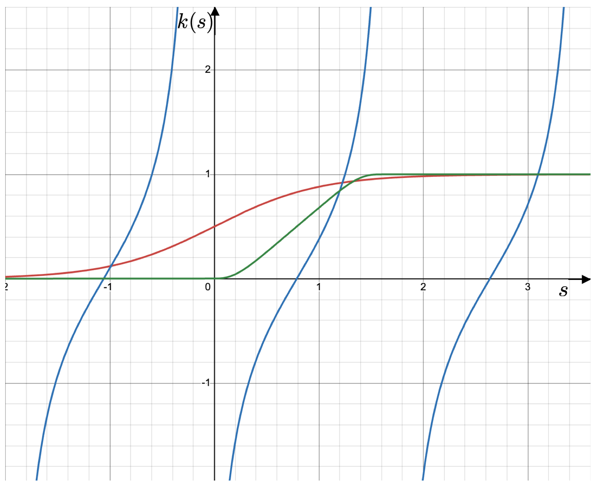
The goal of this paper is to build some tailored functions encoding the shape of the desired path reference profile according to the following logic. The curvature is set in relation to the arc length, $\kappa =\kappa \left(s\right)$, thus expressing its Cesaro equation. Function $\kappa \left(s\right)$ is built as a piecewise function on compact intervals where it takes either one of the constant values between $\{0,\mathsf{\Omega },-\mathsf{\Omega }\}$, or a smooth connection among them that is constructed as the composition of two basic functions $f\left(x\right)$, $g\left(x\right)$, $\kappa \left(s\right)=f\left(g\right(s\left)\right)$, $f\left(x\right)$ being a smooth monotone function from zero to one, and $g\left(x\right)$ set to ‘shrink’ the domain to a desired interval.

Considering the above structure and logic, take the following functions:

$$f\left(x\right)=atanh\left(cx\right)+b$$

(7)

$$g\left(x\right)=tan(dx+f)$$

(8)

with parameters $a,b,c,d,f\in \mathbb{R}$. Function $f\left(x\right)$ smoothly and monotonically connects $b-a$ to $a+b$, so that in the following we set either $a=b={\displaystyle \frac{1}{2}}$ in case of transition from 0 to 1, or $a=1,b=0$ for transition from $-1$ to 1. Function $g\left(x\right)$ monotonically maps the interval $\mathcal{I}=({\displaystyle \frac{-\pi -2f}{2d}},{\displaystyle \frac{\pi -2f}{2d}})$ to the real line. A graphical sketch of these functions is plotted in Figure 2.

By suitably combining the above functions and tuning the related parameters, in the following we consider a curvature profile as

$${\kappa }_{0-1}\left(s\right)=\left\{\begin{array}{c}\hfill 0\phantom{{\displaystyle \frac{1}{2}}\left(tanh(ctan(dx+f\left)\right)\right)}\mathrm{if}s\le {\displaystyle \frac{-\pi -2f}{2d}}\\ \hfill {\displaystyle \frac{1}{2}}\left(tanh(ctan(ds+f)+1)\right)\phantom{0}\mathrm{if}s\in \mathcal{I}\\ \hfill 1\phantom{{\displaystyle \frac{1}{2}}\left(tanh(ctan(dx+f\left)\right)\right)}\mathrm{if}s\ge {\displaystyle \frac{\pi -2f}{2d}}\end{array}\right.$$

(9)

in the case of transition between 0 and 1, thus useful for connecting a straight line to a circle, or:

$$\kappa {\left(s\right)}_{1-1}=\left\{\begin{array}{cc}\hfill -1\phantom{{\displaystyle \frac{1}{2}}\left(tanh(ctan(dx+f\left)\right)\right)}& \mathrm{if}s\le {\displaystyle \frac{-\pi -2f}{2d}}\hfill \\ \hfill \left(tanh(ctan(ds+f\left)\right)\right)\phantom{0}& \mathrm{if}s\in \mathcal{I}\hfill \\ \hfill 1\phantom{{\displaystyle \frac{1}{2}}\left(tanh(ctan(dx+f\left)\right)\right)}& \mathrm{if}s\ge {\displaystyle \frac{\pi -2f}{2d}}\hfill \end{array}\right.$$

(10)

for transitions between $-1$ and 1, thus useful for changing turning direction.

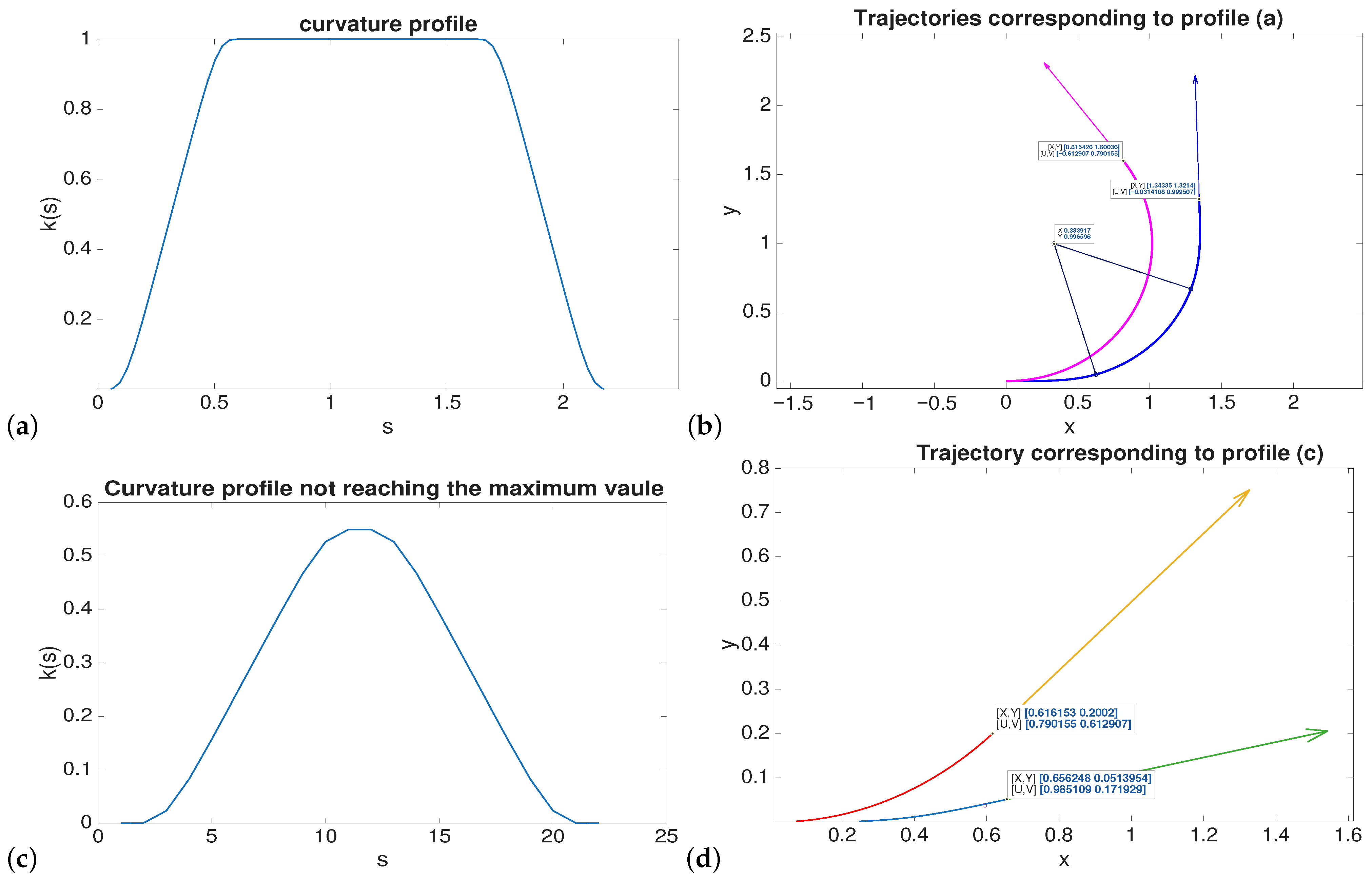
It is worth noting that steering operations not reaching the maximum curvature value are also possible, and the curvature profile adopted for this basic steering in the framework of this paper is:

$${\kappa }_{0-a}\left(s\right)=a·\kappa \left({\displaystyle \frac{s}{a}}\right)$$

(11)

with $a\in (0,1)$, which allows to reach the same maximum derivative of (9) while reducing the maximum value of a.

Functions (9)–(11), together with their mirrored versions ${\kappa }_{1-0}\left(s\right)={\kappa }_{0-1}(-s)$, ${\kappa }_{0-a}\left(s\right)={\kappa }_{a-0}(-s)$, are adopted in this paper as a smooth transition between constant values as described in Section 4.

Discussion on Criteria for Parameters Tuning

Function $\mathcal{F}$ can be tuned through five parameters $a,b,c,d,f$. However, they have a different impact on the curvature profile. Parameters $a,b$ are set to impose the boundary values. Oppositely, parameters $c,d,f$ are set to adjust the curvature shape with respect to arc length and hence they are the way to design the best trade-off among length, feasibility and comfort. More in details, they are set according to the following rules.

Parameters d and f are set to adapt any desired interval to the transition interval $\mathcal{I}$, namely for a prescribed transition interval $\mathcal{I}=\{s_1,s_2\}$ we set $d={\displaystyle \frac{\pi }{s_2-s_1}}$ and $f=-{\displaystyle \frac{\pi }{2}}{\displaystyle \frac{s_2+s_1}{s_2-s_1}}$. Conversely, for a desired function $tan(dx+f)$ to be assigned, the inverse relations

$$\left\{\begin{array}{cc}\hfill s_1& =-{\displaystyle \frac{f+\pi /2}{d}}\hfill \\ \hfill s_2& =-{\displaystyle \frac{f-\pi /2}{d}}\hfill \end{array}\right.$$

(12)

provide the values defining the $\mathcal{I}$. As a general rule, parameter f shifts both $s_1$ and $s_2$ of the same amount, while parameter d sets the distance between $s_1$ and $s_2$, being inverse proportional to $s_2-s_1$ (the higher d, the narrower the interval $s_2-s_1$).

Finally, parameter c magnifies the values provided by $f\left(x\right)$, and it is strictly related to the slope of $\kappa \left(s\right)$. It comes out that both c and d modify the slope of $\kappa \left(s\right)$, the difference between them is that c changes the slope of $f\left(g\right(s\left)\right)$ keeping the same abscissa values, while d scales the x-axis and hence modifies the width of the transition zone.

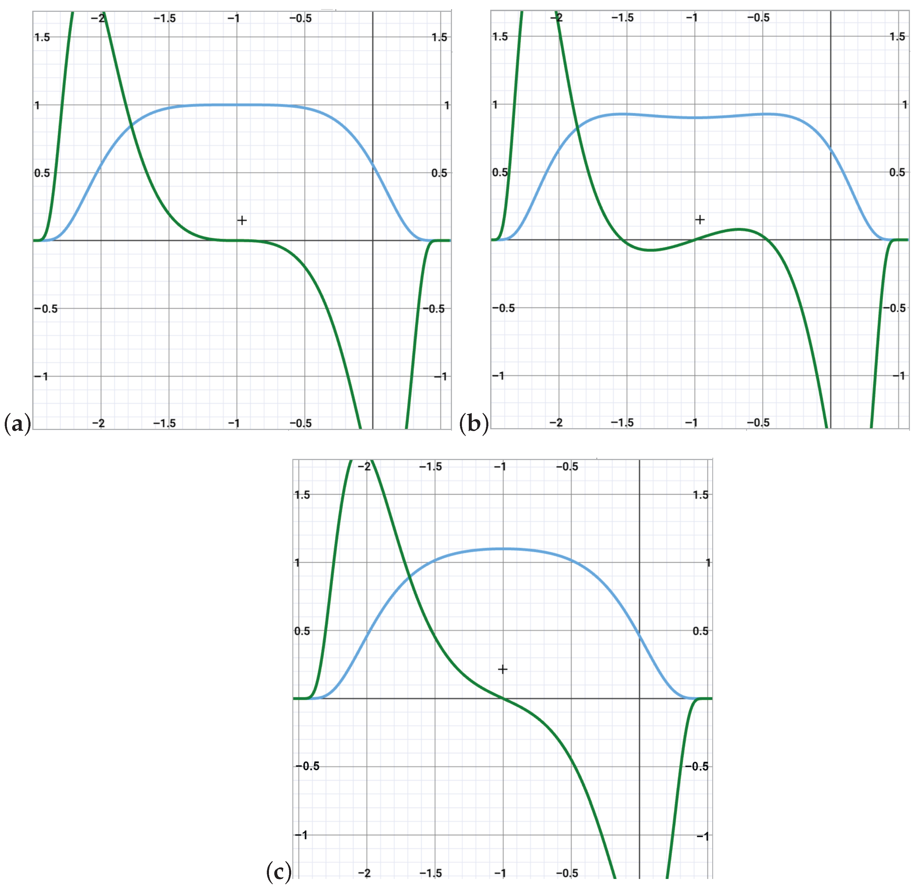
To have a deeper insight, we study the features of the first and second derivative of the transition function (9). The analytical expression is developed in Appendix B, and it is possible to verify that ${\displaystyle \frac{dk\left(s\right)}{ds}}$ is a bump function. Here we discuss the structure of the functions derived in Appendix B through their graph.

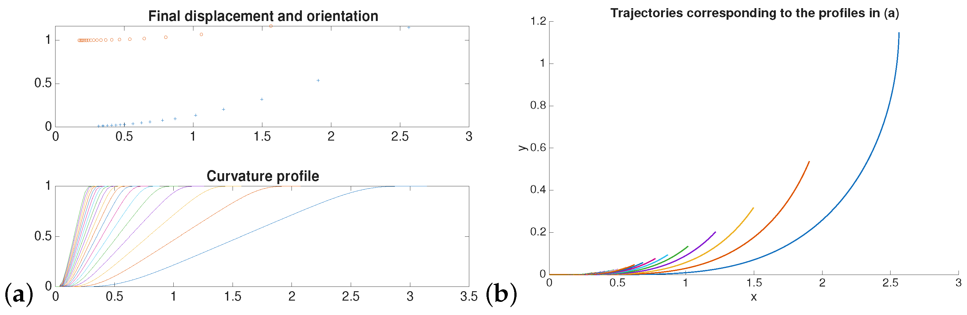
Figure 3 shows the plots of these functions for $c=0.9$, $c=1$ and $c=1.1$. From Equation (A4) and considering the plots in Figure 3, it is easy to see that, for $c\ge 1$, ${\displaystyle \frac{dk\left(s\right)}{ds}}$ has one single maximum equal to $acd$ in the midpoint of $[s_1,s_2]$, or equivalently ${\displaystyle \frac{d^{2}k\left(s\right)}{d{s}^2}}$ has one only zero crossing, otherwise ${\displaystyle \frac{dk\left(s\right)}{ds}}$ has multiple stationary points and ${\displaystyle \frac{d^{2}k\left(s\right)}{d{s}^2}}$ several zero crossings. In terms of curvature shape, this implies that function $f\left(g\right(s\left)\right)$ has a single inflection point at the midpoint of $[s_1,s_2]$ in the interval for $c\ge 1$, otherwise not.

Starting from the above discussion, we now describe the tuning criteria for $a,b,c,d,f$ in order to build a function $\mathcal{F}\left(s\right)$ which is compliant with the motion generation and planning system contraints in a common case, the other cases can be treated analogously. Consider that we are interested in selecting a curvature profile as in (9) that is compliant with the constraints

$$\left\{\begin{array}{c}\kappa \left(s\right)\le \overline{k},\hfill \\ {\displaystyle \frac{d}{ds}}k\left(s\right)\le \overline{\sigma },\hfill \\ {\displaystyle \frac{d^2}{d{s}^2}}k\left(s\right)\le \overline{\rho },\hfill \end{array}\right.$$

(13)

which encode the geometry of a turn. Considering the first constraint and thus transitions of $k\left(s\right)$ from 0 to $\overline{k}$, we set $b-a=0$ and $a+b=\overline{k}$, so that $a=b={\displaystyle \frac{\overline{k}}{2}}$.

As for ${\displaystyle \frac{d}{ds}}k\left(s\right)\le \overline{\sigma }$, observe that, in view of the above discussion, for $c\ge 1$ it holds ${\displaystyle \frac{d}{ds}}k\left(s\right)\le acd$, so that imposing $acd\le \overline{\sigma }$ makes the second constraint of (13) satisfied. Overall, first and second relation are compactly expressed by $cd\le {\displaystyle \frac{2\overline{\sigma }}{\overline{k}}}$. As for the last constraint of (13), from (A5) in Appendix B it is possible to state that ${\displaystyle \frac{d^2}{d{s}^2}}k\left(s\right)\le \alpha d^2{c}^2$ where $\alpha$ is a constant that can be handily computed, and this in turn reveals that imposing $\alpha d^2{c}^2\le \overline{\rho }$ makes also the third constraint of (13) satisfied.

To keep all the above relations compact, define $\mathsf{\Xi }=max\{{\displaystyle \frac{4{\overline{\sigma }}^2}{{\overline{k}}^2}},{\displaystyle \frac{\overline{\rho }}{\alpha }}\}$, that allows to encode both the second and the third contraint into the relation $d^2{c}^2\le \mathsf{\Xi }$. Now, considering that it is better to impose $c\ge 1$ and that Equation (12) expresses that a larger d corresponds to a thinner transition width (which is equal to $\pi /d$), a possible set of parameters satisfying (13) is:

$$\left\{\begin{array}{c}a=b={\displaystyle \frac{\overline{k}}{2}},\hfill \\ c=1,\hfill \\ d={\mathsf{\Xi }}^{1/2},\hfill \\ \mathsf{\Xi }=max\{{\displaystyle \frac{4\overline{{\sigma }^2}}{{\overline{k}}^2}},{\displaystyle \frac{\overline{\rho }}{\alpha }}\}.\hfill \end{array}\right.$$

(14)

The above set of parameters allows the path-planning algorithm to generate reference trajectories compliant with the set of constraints (13), and it turns to guarantee prescribed levels of comfort and inertial stress of the structure encoded by a cost function as in (6). It is worth remarking that the above setting is just one of the possible choices, and we believe that our framework provides tools for a wide set of possibilities, according to diverse control goals, and this reveals the flexibility of the proposed approach.

4. Smooth Approximation of a Dubins Path

In this section, we exploit the functions previously introduced to compute any Dubins path. As a first step, we analyzed the geometry of a steering operation associated to a curvature profile as in (9). The outcome of this analysis constitutes the basic block for the proposed smooth approximation.

Geometry of a Turn Associated to a Curvature Profile as in (9)

We start the analysis comparing the motion of a rectangular curvature shape with the proposed smooth profile (9). Figure 4a shows the curvature profile for a left turn to reach the maximum curvature starting from zero, which corresponds to the graph of (9) for $c=1$, $d=\pi$, $f={\displaystyle \frac{\pi }{2}}$. In Figure 4b the motion of either an ordinary Dubins vehicle is plotted when moving according to $0-1$ curvature (red line), and that of a vehicle following curvature profile as in Figure 4a. It is interesting to note the displacement and direction deviations, respectively equal to $(0.755,0.327)$ with $\theta =55.8°$ for the Dubins vehicle and $(0.958,0.115)$ with $\theta =26.25°$, so basically the motion corresponding to Figure 4a is flattened to the x-axis, and the angle is reduced nearly to half of the Dubins path. This shifting is more evident considering Figure 5, where the displacement of the final point at maximum curvature is plotted (+ symbol) together with the center of the left Dubins circle (o symbol) for several values of parameter d.

Figure 6 is related to the geometry of a left turn from the maximum to zero, thus following either the curvature profile ${\kappa }_{1-0}\left(s\right)$ depicted at the top of Figure 6a that we use for large turns, or ${\kappa }_{a-0}\left(s\right)$ as in Equation (11), which is adopted when dealing with small turns. Figure 6b shows the plot of a family of positions and orientations achieved for the curvature profiles Figure 6a, where it is assumed that the vehicle starts with maximum steering and which are divided between large turns, where the curvature is kept to the maximum value for a variable amount of time, and short turns, that are characterized by Equation (11) for several values of a. Red vectors denote positions and orientations relative to small turns obtained following profiles Equation (11).

Figure 7 shows positions and orientations of a vehicle following the Figure 4a profile and keeping the final curvature, namely a ’mirrored’ curvature with respect to the profiles in Figure 6a.

In Section 5, it turns out that the two figures Figure 6b and Figure 7 are a powerful graphical description of the geometry of a basic left turn respectively reaching or starting from the straight line, and we make use of them in Section 5 for the construction of reference paths.

Finally, we consider a full regular turning operation starting and returning to the zero curvature. Two types of turning profiles are possible depending on the total amount of steering angle, namely reaching and keeping the maximum turning radius, or not. Two examples of such profiles are depicted in Figure 8, where the plots on the top refer to a steering manouver for a large turning angle. In this case, the maximum curvature is reached and kept for a suitable time. In the figures below, an example of a small turn is depicted, the curvature profile in this case does not reach the maximum value.

As a final remark, analogously to Figure 6 and Figure 7, we graphically describe the geometry of these full regular turning operations through the computation of positions and orientations achieved for a family of curvature profiles, both for small and large turns. Those corresponding to small turns, not reaching the maximum curvature value, are depicted in red. Aside from the importance of these graphs themselves, it comes out that they constitute a fundamental tool for the investigation of Section 5.

5. Path Planning Design

Starting from the analysis developed in the previous Section, we now derive an algorithm to build the reference path profile for each of the two basic problems described in the Problem Statement.

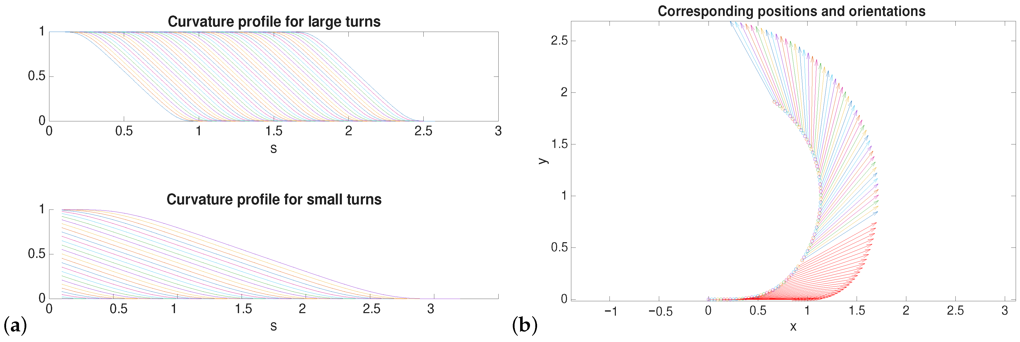
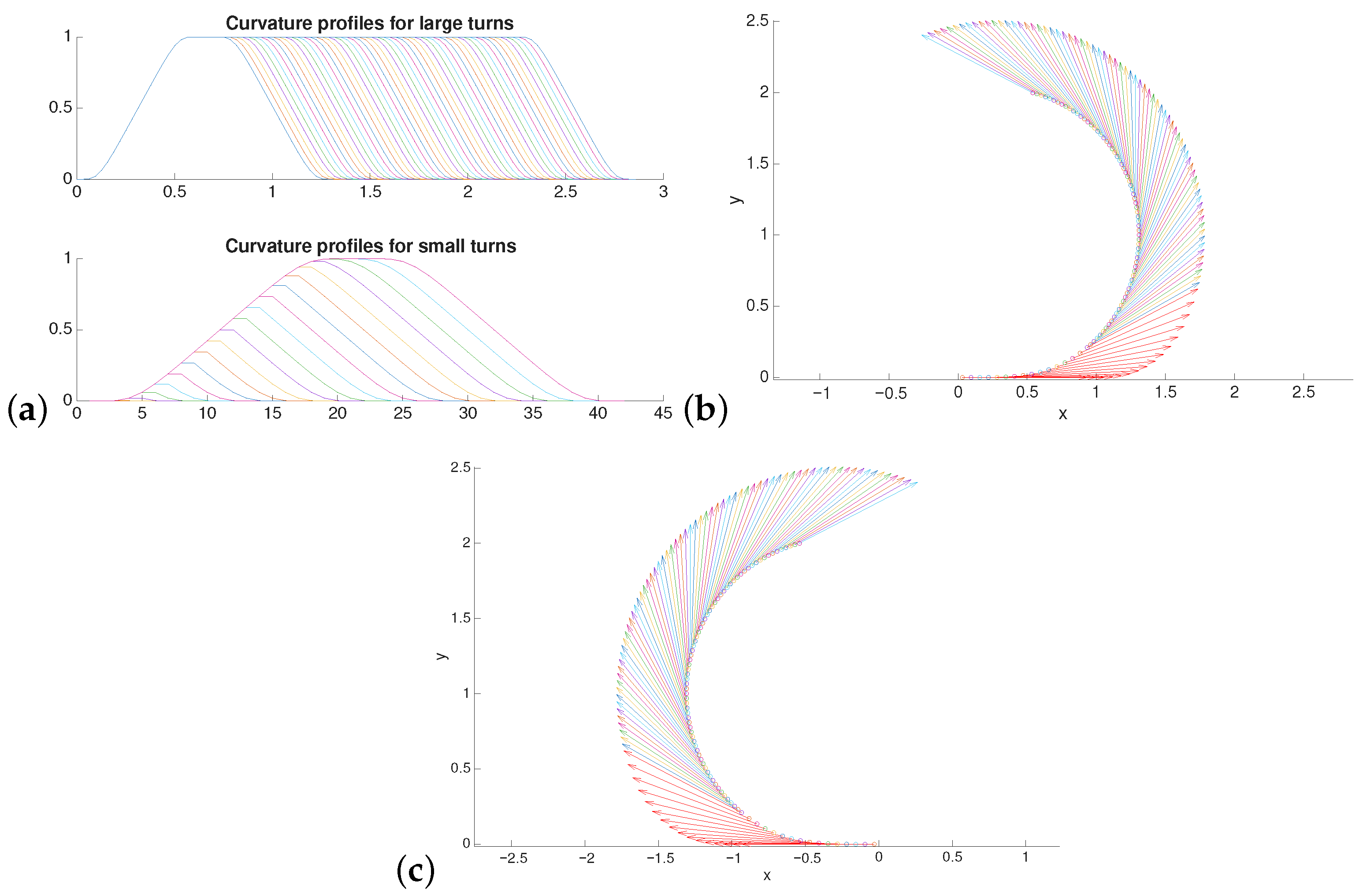
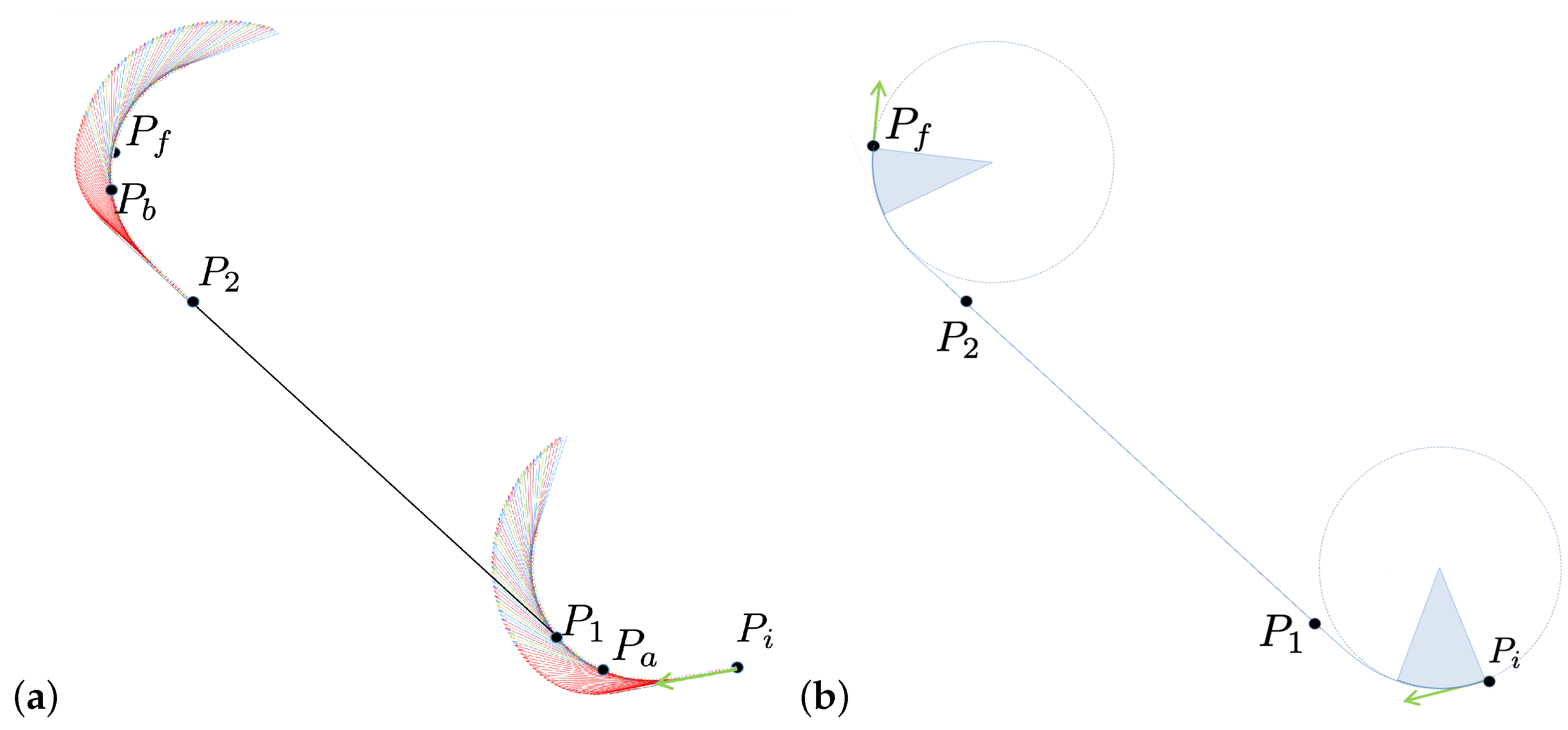
We start from Problem 1. Here we describe how to graphically sketch the solution from the geometry of the turn described in the previous section exploiting the turning profile depicted in Figure 9b for left turns and Figure 9c for right turns, and then we describe the instructions to get a numerical solution through an appropriate algorithm.

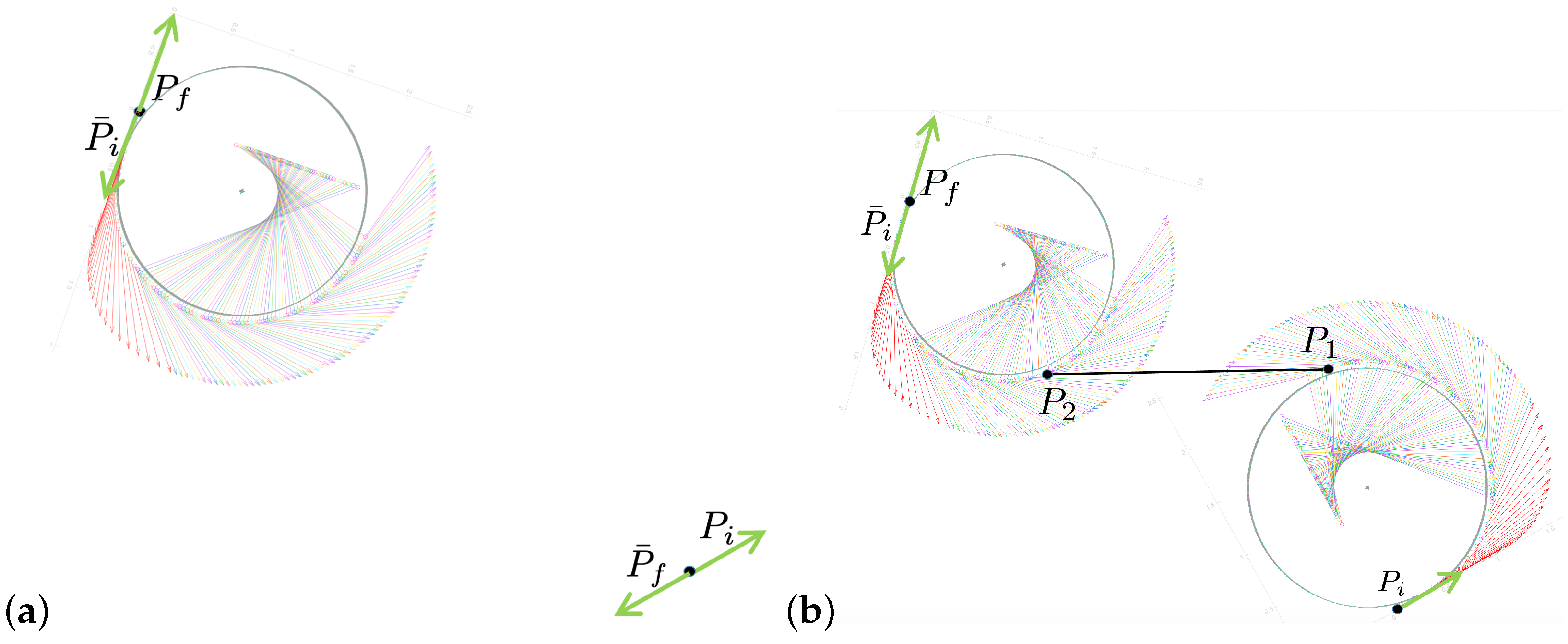
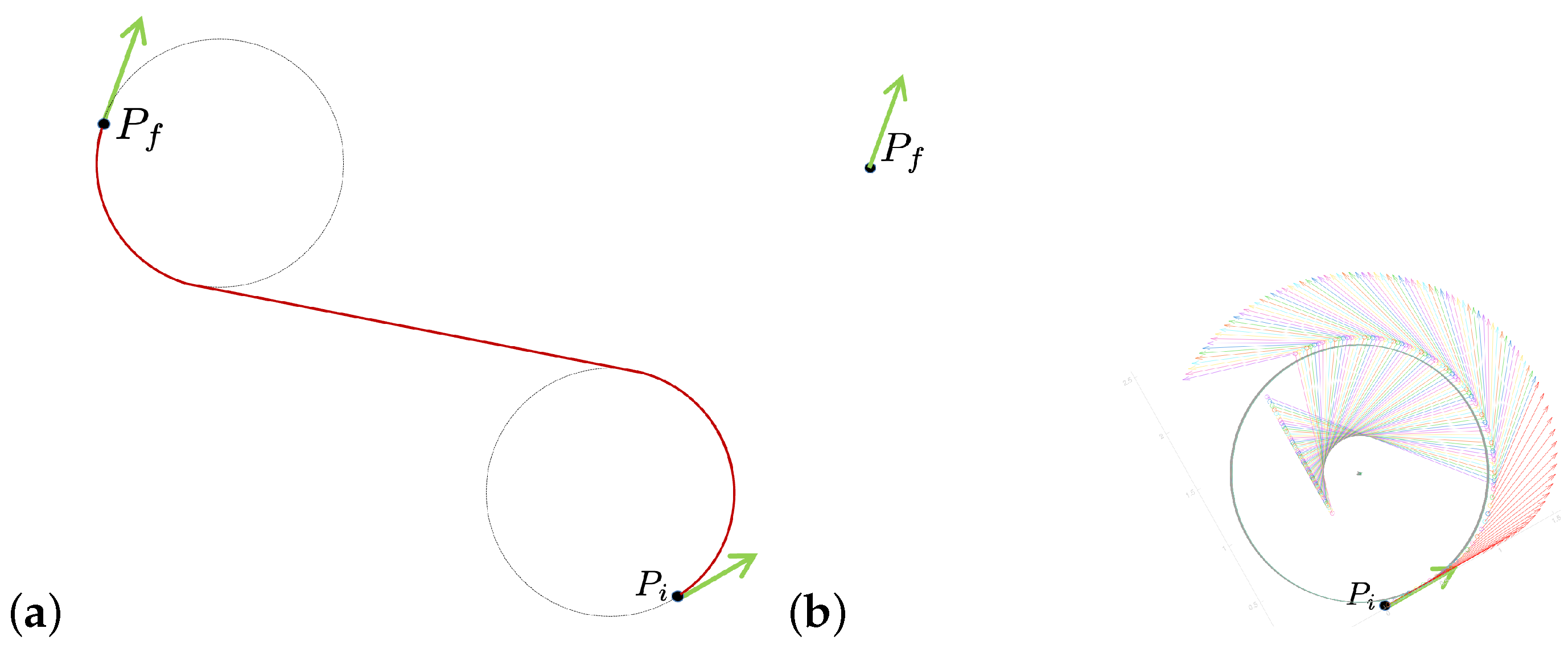
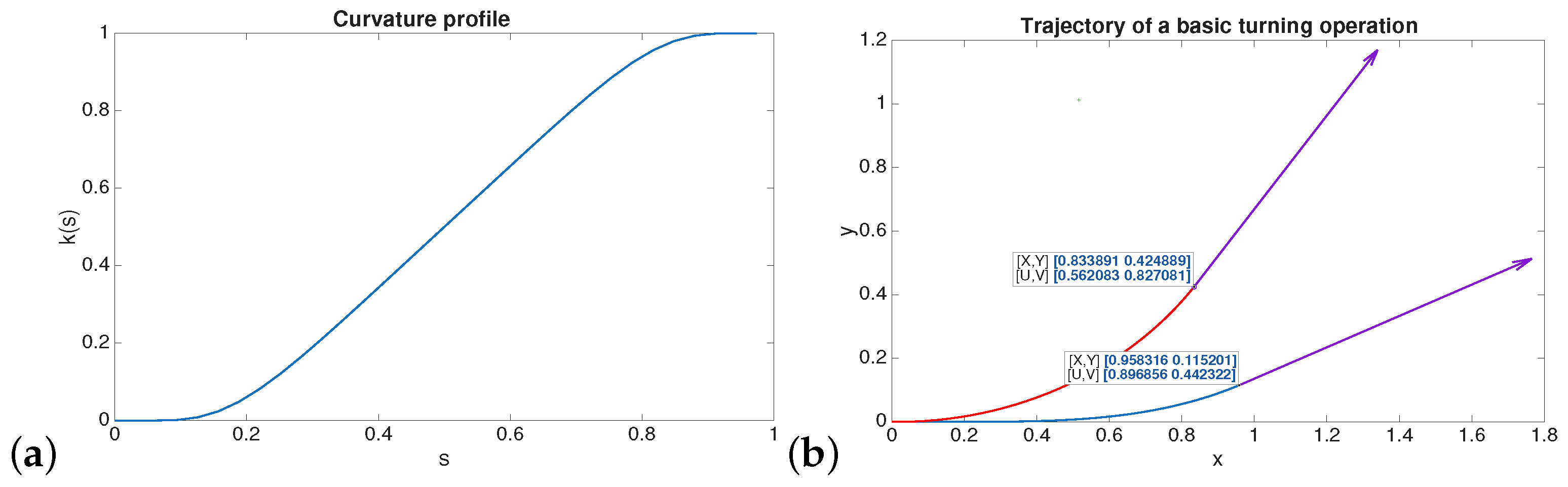
Consider Figure 10a, where two points in the plane, ${\mathbf{P}}_i$ and ${\mathbf{P}}_f$, together with their orientations, are fixed. Assume that a preliminary analysis on the Dubins path type has been performed, with solution LSR, denoted in the figure with the red line. Under the assumption that the curvature and its derivative are zero at initial point, and considering that the first part is a left turn, positions and orientations achieved adopting the curvature profile ${\kappa }_{0-1}\left(s\right)$ are given by the vector sum of the initial pose and any of the vectors describing the motion relative to the curvature profile ${\kappa }_{0-1}\left(s\right)$ depicted in 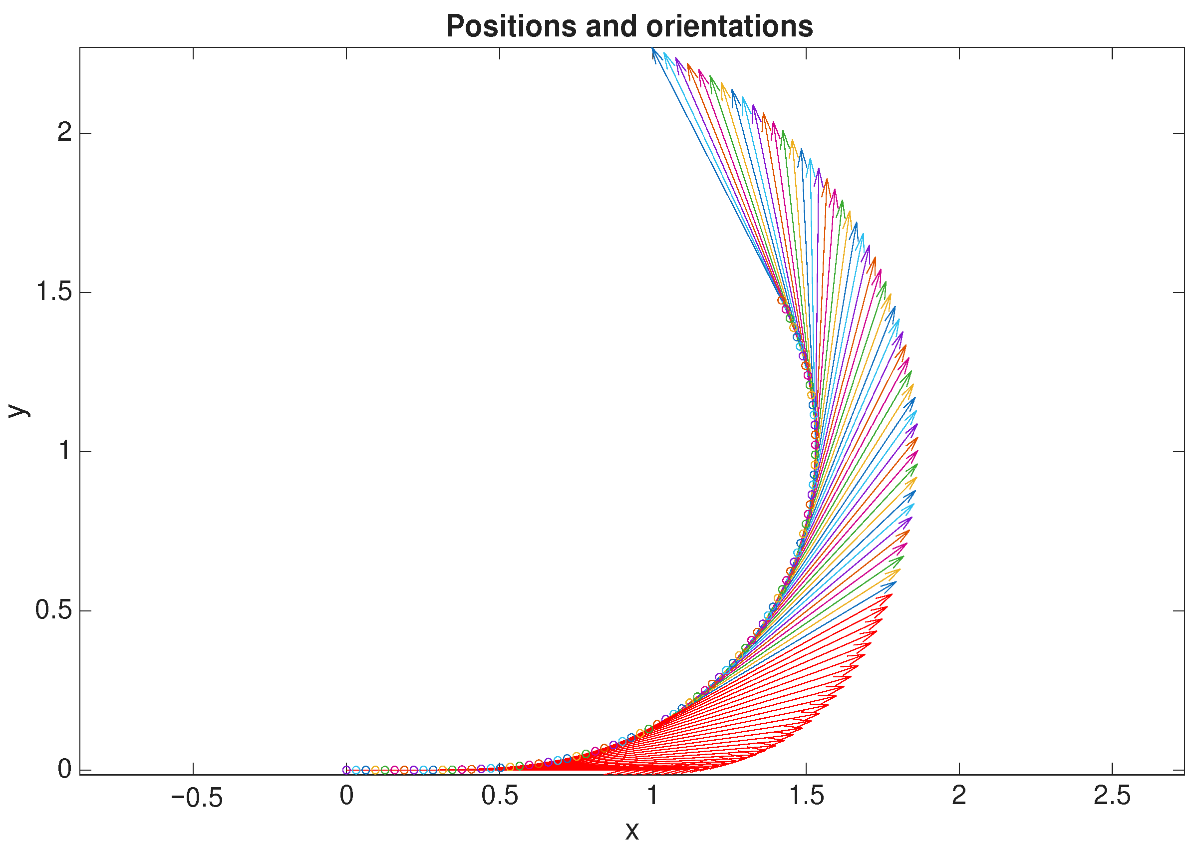Figure 7. For this reason, we make a roto-translation of all the vectors in Figure 7 centered at ${\mathbf{P}}_i$, so that we graphically describe the motion starting from $P_i$ with variable curvature profile (Figure 10b). The first part is a full left turn, positions and orientations achieved adopting the curvature profile in Figure 9a are given by the vector sum of the initial pose and any of the vectors describing the motion relative to the curvature profile depicted in Figure 9b. For this reason, we make a roto-translation of all the vectors in Figure 9b centered at ${\mathbf{P}}_i$, so that we graphically describe the motion starting from $P_i$ with variable curvature profile (Figure 10b).

As a further step, consider that the Dubins path connecting ${\mathbf{P}}_i$ and ${\mathbf{P}}_f$ with orientations ${\phi }_i$ and ${\phi }_f$ coincides with the Dubins path connecting ${\mathbf{P}}_f$ and ${\mathbf{P}}_i$ with orientations $-{\phi }_f$ and $-{\phi }_i$. Indeed, the same path can be travelled from ${\mathbf{P}}_i$ to ${\mathbf{P}}_f$ or backwards from ${\mathbf{P}}_f$ to ${\mathbf{P}}_i$, with opposite orientation. For this reason, in Figure 11a we make also a roto-translation of all the vectors in Figure 7 centered at ${\mathbf{P}}_f$ with opposite orientation (denoted as ${\overline{\mathbf{P}}}_f$ in Figure 11b).

To get the solution, we focus on the central straight ‘S’ part of the Dubins path. In its smooth approximation, the central line must connect the point where the first turning operation ends (that we denote as $P_1$ in Figure 11b) to the point where the second turning operation starts. From a graphical perspective, the solution is obtained as follows. Take one point ${\overline{P}}_1$ on ${\mathcal{C}}_{P_i}$, another one ${\overline{P}}_2$ on ${\mathcal{C}}_{{\overline{P}}_f}$, select those satisfying:

$$\phi \left(P_1\right)=-\phi \left(P_2\right)={\theta }_{12},$$

(15)

where ${\theta }_{12}$ is the orientation of the line connecting $P_1$ and $P_2$, $\phi \left(P_1\right)$ the orientation in $P_1$.

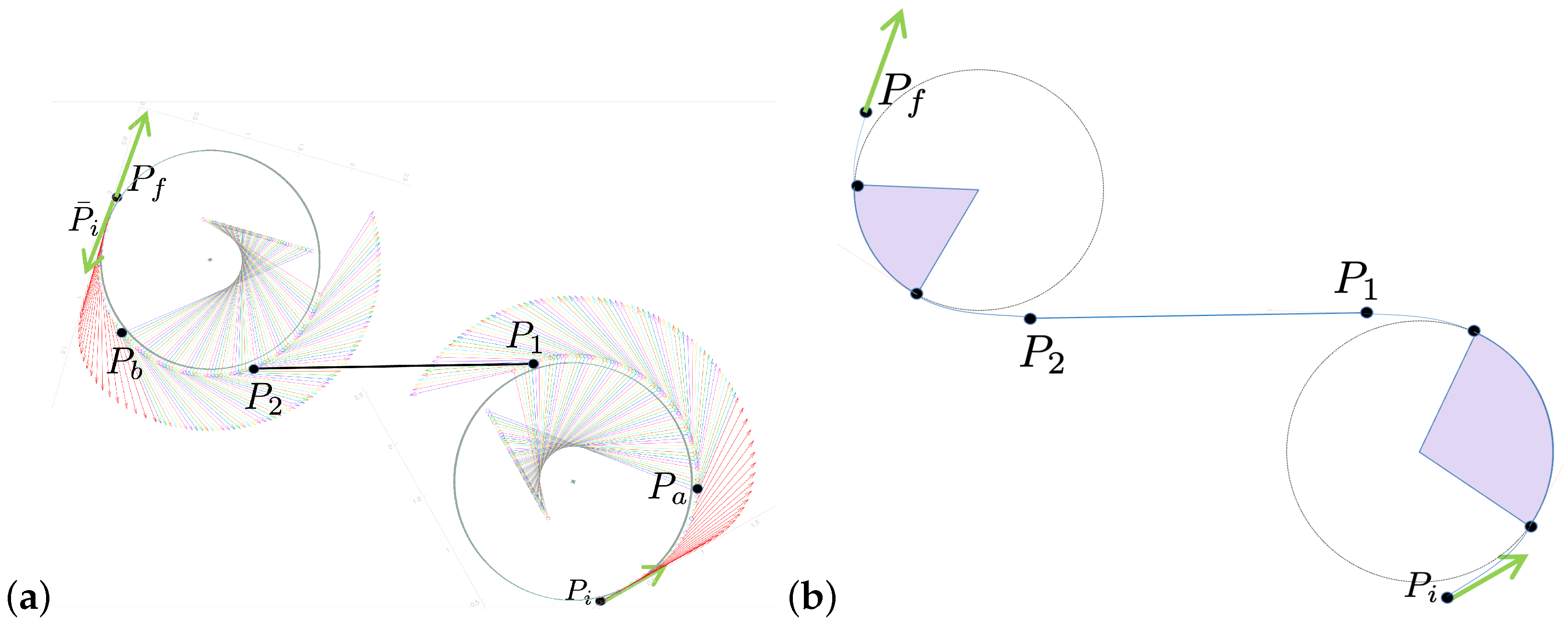
As a final parameter to get the final solution, we can deduce the angle that it is necessary to travel when the maximum curvature is reached (or which profile for small turn must be selected if the maximum curvature is not reached). Consider first the case that the graphical solution provides $P_1$ and $P_2$ which are not the red vectors, and denote with $P_a$ the last red vector (which corresponds to the curvature touching but not keeping the maximum curvature, which separates the small turn profiles from large turns profiles). It is easy to see that the angular distance between $P_1$ and $P_a$ is equal to how much the curvature must be kept equal to the maximum in the first turn, and analogously the angular distance between $P_2$ and $P_b$ with respect to the second turn.

On the other hand, if the solution above allows to select either $P_1$ or $P_2$, or both or them, in the red part, the distance of $P_1$ from $P_a$ (or $P_2$ from $P_b$) allows to select the appropriate curvature profile for small turns which solves the problem.

The final solution is depicted in Figure 12b.

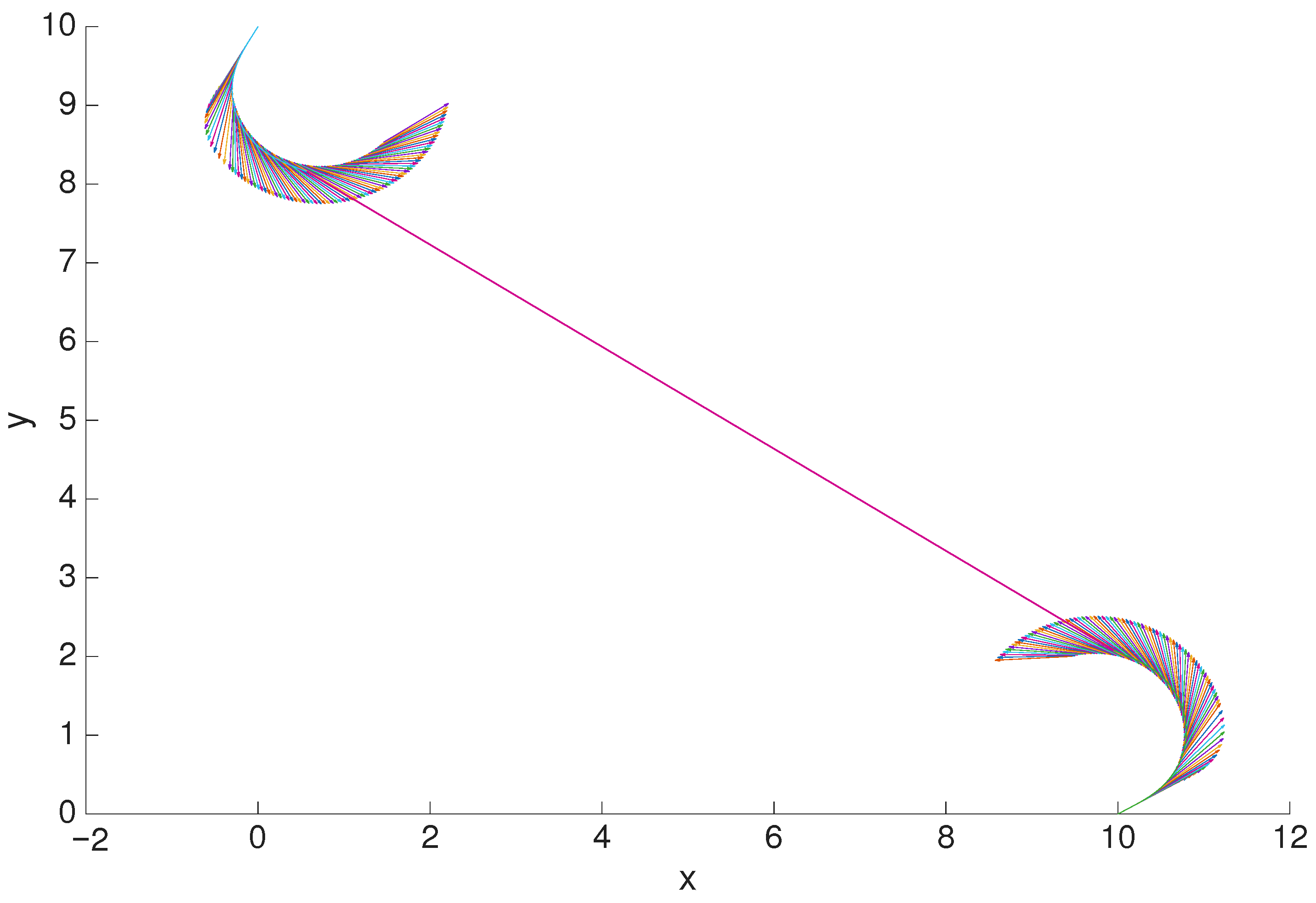
We now describe the steps to follow to pursue the problem solution through a numerical approach. Figure 13 displays the solution sought through a numerical routine that we use in the following to describe the steps of the algorithm in general. The initial and final poses are equal to $P_i=(10,0)$ and $P_f=(0,10)$, with orientation respectively ${\varphi }_i={30}^{\circ }$ and ${\varphi }_f={60}^{\circ }$.

A preliminary step is the construction of a matrix ${\mathcal{C}}_l\in {\mathbb{R}}^{3\times (N+M)}$ encoding the directions and orientations for variable curvature values, as graphically depicted in Figure 9b. We assume that N is a uniform subdivision of a total angle $\alpha$ where the solution belongs to (usually between $\pi /2$ and $\pi$), so that column $N+i$ of ${\mathcal{C}}_l$ encodes position and angle for a steering of an angle equal to $i·{\displaystyle \frac{\alpha }{M}}$ computed through Equations (A1)–(A3). We assume the same for small turns, where the positions and orientations are computed for a set of N curvature profiles having maximum value equal to ${\displaystyle \frac{k}{N}}·i$.

As a first step, we make a roto-translation of positions and orientations stored in ${\mathcal{C}}_l$ at $P_i=(10,0)$, in order to center them at $P_i$ with orientation ${\varphi }_i={30}^{\circ }$ as follows. Denoting by ${\mathbf{x}}_{{\mathcal{C}}_l}$ the first two rows of ${\mathcal{C}}_l$ and by ${\mathit{\varphi }}_{{\mathcal{C}}_{\mathbf{l}}}$ its third row, representing respectively positions and orientations of Figure 9b, then ${\mathbf{x}}_{{\mathcal{C}}_i}={\mathcal{R}}_l{\mathbf{x}}_{{\mathcal{C}}_l}+{\mathbf{x}}_{P_i}$, where ${\mathbf{x}}_{{\mathcal{C}}_i}$ are the values of positions and orientations after the roto-translation, and ${\mathcal{R}}_l$ is the rotation matrix defined as ${\mathcal{R}}_l=\left[\begin{array}{cc}cos\left({\varphi }_i\right)& -sin\left({\varphi }_i\right)\\ sin\left({\varphi }_i\right)& cos\left({\varphi }_i\right)\end{array}\right]$. Next, we do the same at the reversed final position, namely at $P_f$ with orientation ${\varphi }_i=-{60}^{\circ }$.

Then we take one point ${\overline{P}}_1$ on ${\mathcal{C}}_{P_i}$, another one ${\overline{P}}_2$ on ${\mathcal{C}}_{{\overline{P}}_f}$ and we impose (15); in the example depicted in Figure 13 we found $i=65$ for the point on ${\mathcal{C}}_{P_i}$, and $j=48$ for the point on ${\mathcal{C}}_{P_f}$, and considering that the step was set equal to $\pi /100$, it results that the first turning angle is equal to $0.65 \pi$ and the last is $0.48 \pi$.

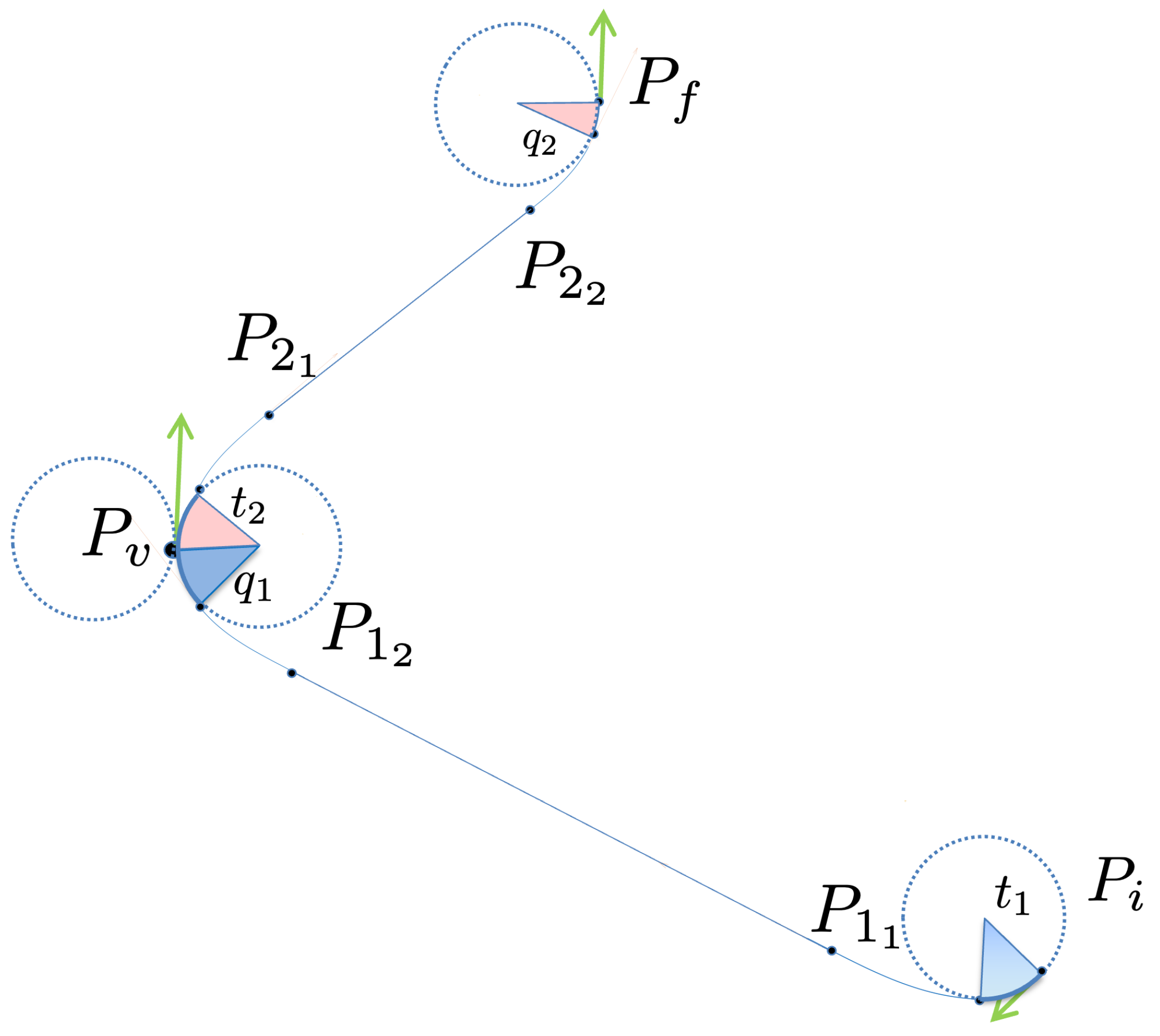
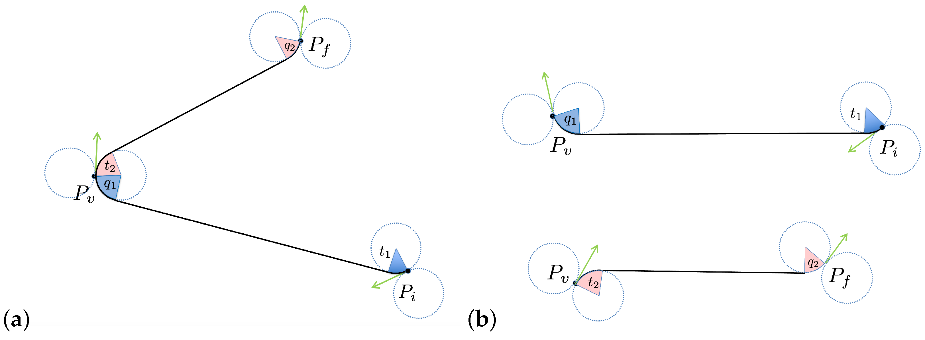
Consider now Problem 2. A basic problem in this framework is to select the smooth curve approximating the Dubins path connecting $P_i$ or $P_f$ considering fixed orientations and free curvature and curvature derivative. The solution to this problem can be computed both graphically and numerically following the above steps that lead to the solution of Problem 1, with the only difference of using positions and orientations depicted in Figure 5b when dealing with curvature ${\kappa }_{1-0}\left(s\right)$ at the initial position or Figure 6 for ${\kappa }_{0-1}\left(s\right)$ used at the final position. Figure 14a shows the construction of the graphical solution. Denote by t the angular distance between $P_a$ and $P_1$, and by q the one between $P_b$ and $P_2$.

The most interesting fact is that the above solution is useful to solve the general Problem 2.

Before describing the construction of the solution in the general case of n points $P_i$, we state one main optimality principle which is widely adopted when dealing with the n points Dubins problem, that we extend also in the case of smooth paths.

The following Statement is a corollary proved in [33]. The same principle has been assumed to hold for the general n-points Dubins problem in [34].

Property 1. 

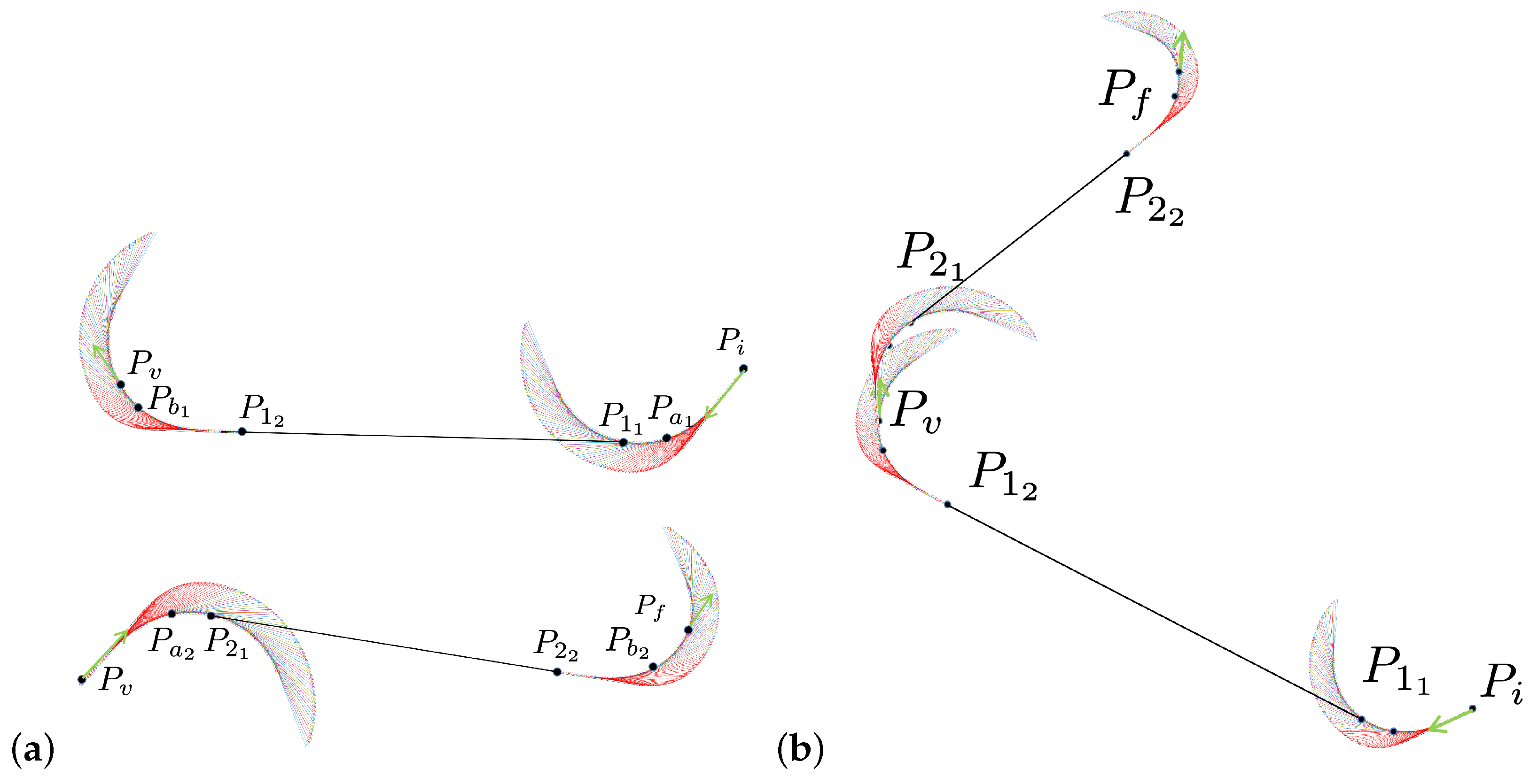
The length-optimal path has the following property. Optimal paths never have a change of curvature at the crossing of a via point. The final turning angle of the first subpath is equal to the first turning angle of the second subpath (i.e., $q_1=t_2$ in Figure 15).

Consider the problem of interconnecting three points, the middle being with free orientation (the so called 3PDP problem). Figure 15a shows the optimal solution with discontinuous curvature as deduced in [35], which is characterized by the fact that the angle $q_1=t_2$. Considering that the crossing of a via point $P_v$ requires a full turning operation, from a straight line to a different straight line, it is possible to divide the problem into two, one focused on the smooth path between $P_i$ and $P_v$, the other between $P_v$ and $P_f$, with the additional constraint that $q_1=t_2$, as depicted in Figure 15b. Moreover, since the most reasonable turning at the via point requires that the crossing of $P_v$ is made at the maximum curvature, each of the two splitted sub-problems have the structure of a basic Problem 2 (see Figure 16a). To get the final solution, the two sub-problems are then merged together at the via point (see Figure 16b) to finally get the final solution path as depicted in Figure 17. Moreover, this same strategy is adopted for the general n-points Dubins Problem.

In general, the n-points Dubins Problem is solved by recurring to any algorithm providing the solution for the ordinary Dubins vehicle (as the one in [34]), and then constructing the smooth approximation expoiting the strategy described above, and thus converting the original problem into a $(n-1)$ basic Problem 2.

6. Conclusions

In this paper, the use of a tunable, smooth curvature function for path planning of Dubins vehicle is thoroughly investigated. This study is motivated by the importance of a path-planning algorithm to produce curvature profiles which can be effectively tracked by the vehicle through a suitable control algorithm. After a wide discussion of the features and drawbacks of the approaches already available in the scientific literature, the problem setting is introduced, and two basic problems are stated in order to solve a wide variety of cases of interest. Next, a detailed analysis is performed regarding a smooth tunable compact function that is further exploited to generate a smooth transition between constant curvature values. The resulting methods are graphical and thus effective for real-time applications, and the structure of the algorithm is finally described to generate the reference path profile by machine computation.