Research on Green Flexible Job Shop Rescheduling with Urgent Order Insertion and Multi-Speed Machines: A Model and an Improved MOEA/D Algorithm

Abstract

This paper investigates a tri-objective green flexible job shop rescheduling problem under urgent order insertion and multi-speed machining conditions, where makespan, total energy consumption, and total tool wear are jointly optimized. First, an event-driven freezing mechanism is introduced, in which completed and ongoing operations are fixed, while only the rescheduling window composed of waiting operations and urgent-order operations is re-optimized. On this basis, two rescheduling strategies, namely complete rescheduling and deferred rescheduling, are designed and compared. Second, to improve the solution capability in complex dynamic environments, an improved multi-objective evolutionary algorithm based on decomposition (IMOEA/D) with a three-layer encoding scheme is proposed. The algorithm incorporates hybrid initialization, tabu-guided crossover, simulated annealing mutation, and critical-path-based variable neighborhood search. Experimental results show that the proposed method performs well in energy consumption optimization and tool wear control, while effectively improving the diversity and distribution quality of the Pareto solution set. Further analysis indicates that deferred rescheduling generally outperforms complete rescheduling, while the original-orders-first and urgents-first strategies exhibit different strengths in convergence, solution quality, and objective optimization. The proposed study provides an effective modeling and optimization framework for multi-objective green rescheduling problems and offers theoretical support for production scheduling decisions that need to balance production efficiency, energy saving, and tool-related cost control in practical manufacturing systems.

1. Introduction

With the aggravation of environmental issues and the rise in energy costs, manufacturing enterprises are paying increasing attention to green scheduling and energy efficiency [1]. Scheduling decisions directly affect makespan and energy consumption by reshaping machine busy/idle patterns, processing sequences, and resource utilization. Meanwhile, under high-mix low-volume production and fast delivery requirements, job shops are frequently exposed to dynamic disruptions such as urgent order insertion, making it necessary to adjust the original plan rapidly while maintaining schedule stability [2]. Unlike the traditional static flexible job shop scheduling problem (FJSP), multi-speed machining requires each operation to determine not only an eligible machine but also a speed level: higher speeds usually shorten processing time, yet may increase power demand and tool wear, leading to a complex trade-off among makespan, energy consumption, and tool wear.

This paper investigates a green flexible job shop rescheduling problem with urgent order insertion and multi-speed machines. Operation sequencing, machine assignment, and speed selection are jointly optimized with three objectives: minimizing makespan (${\mathrm{C}}_{\mathrm{m}\mathrm{a}\mathrm{x}}$), total energy consumption (E), and total tool wear (W). A Pareto solution set is provided to support decision makers in selecting appropriate trade-off schedules.

The main innovations and contributions of this paper are as follows:

• Model contribution: a tri-objective green rescheduling model is developed by integrating urgent order insertion and multi-speed machining into a unified framework.
• Mechanism contribution: an event-driven freezing rule is proposed, and the differences between two rescheduling policies—complete rescheduling and right-shift rescheduling—are systematically compared.
• Algorithm contribution: a three-layer-encoding IMOEA/D is proposed, incorporating hybrid initialization, tabu-guided crossover, simulated annealing mutation, and critical-path-based VNS [3].

The remainder of this paper is organized as follows. Section 2 reviews related studies. Section 3 describes the problem and rescheduling strategies. Section 4 presents the mathematical model. Section 5 introduces the proposed IMOEA/D algorithm. Section 6 reports the experimental design and results. Section 7 presents an industrial case study and discusses future work.

2. Related Work

Recent reviews have shown that dynamic manufacturing scheduling is increasingly studied from the perspectives of trigger events, rescheduling scope, implementability, and real-time decision mechanisms [4]. In particular, recent studies emphasize the importance of event-driven rescheduling, digital monitoring [5], and the comparison between different rescheduling strategies under practical disturbances such as order insertion and machine failures [6].

Recent studies on green flexible job shop scheduling have explicitly incorporated machine idle states, speed-level selection [7], setup/transportation effects [8], and broader energy-related criteria into scheduling models, showing that energy-aware scheduling should not be limited to processing energy alone.

Regarding tool wear and multi-speed machining, Tian et al. developed a model considering both tool degradation and energy-saving measures, treating tool wear as a crucial cost factor that is closely linked to energy consumption [9]. This approach offers a verifiable paradigm for integrating wear into green optimization objectives. However, many studies primarily use multi-speed machining to strengthen the trade-off between makespan and energy consumption. When dynamic disturbances, such as urgent order insertion, occur, the reconstruction of critical paths triggers the need to rebalance speed strategies, redistributing wear accumulation and energy consumption. However, a comprehensive understanding of the dynamic relationship between speed strategies, tool wear, and energy use under such disturbances remains lacking.

In recent years, learning- or data-driven scheduling methods have garnered attention for offering more flexible and adaptive solutions to complex scheduling problems. Techniques like machine learning, reinforcement learning, and neural networks are increasingly applied to dynamically adjust scheduling decisions based on real-time data and past experiences. These methods show great potential in addressing the evolving nature of dynamic events and optimizing scheduling decisions in environments where traditional optimization models may fall short. International research on dynamic flexible job shops increasingly frames rescheduling as a multi-objective decision problem that must respond to disruptions (e.g., new job/rush-order arrivals and machine unavailability) while explicitly controlling energy use [10]. Caldeira et al. formulated an energy-conscious flexible job shop scheduling problem with new job arrivals and a machine turn-on/off strategy, and proposed an insertion-based rescheduling mechanism that jointly minimizes makespan, energy consumption, and schedule instability. In parallel, Naimi et al. showed that reinforcement learning can be leveraged to select rescheduling actions in flexible job shops while balancing energy and productivity objectives [11]. Beyond algorithmic frameworks, discrete-event formalisms such as Petri nets have also been employed to represent interruption events and drive schedule-repair logic at the system level [12]. Moreover, energy-aware scheduling is increasingly extended from “processing energy” alone to system-level indicators such as real-time energy cost, peak demand, and emission-related metrics [13], emphasizing that energy management can be embedded directly into the scheduling formulation.

A complementary research stream integrates cutting-tool condition into scheduling. Because tool deterioration progressively changes machining efficiency, it can prolong effective processing times, raise energy use, and increase tooling-related costs—so tool replacement timing becomes intertwined with sequencing decisions. Salama and Srinivas modeled job sequencing together with tool replacement activities and minimized a composite cost that includes energy, tooling, and tardiness, illustrating how sustainability criteria reshape classic scheduling formulations [14]. Recent studies have increasingly treated tool-related decisions as endogenous scheduling factors rather than fixed exogenous conditions [15].

Nevertheless, a clear research gap remains in jointly addressing tool-wear dynamics within disruption-driven rescheduling in flexible job shops, especially when processing speeds are adjustable. In such settings, inserting a rush order or repairing a breakdown may change the critical path and trigger a reallocation of speed decisions, which in turn redistributes both wear accumulation and energy use across operations; capturing this coupling requires models and solution methods that go beyond static wear assumptions. This motivates adaptive and learning-based approaches capable of updating rescheduling policies online as shop-floor states evolve. Recent work on explorative reinforcement-learning rescheduling agents demonstrates how near-optimal decisions can be generated rapidly while explicitly controlling schedule nervousness [16], and recent surveys document the growing use of reinforcement learning for production scheduling [17]—while also highlighting reliability and robustness issues that must be addressed for real-world deployment [18].

3. Problem Description and Rescheduling Policies

3.1. Problem Description

Consider a flexible job shop consisting of m machines with discrete speed levels, processing $n$ jobs [19]. Each job ${\mathrm{J}}_{\mathrm{i}}$ is composed of a set of operations subject to given technological precedence constraints. For any operation ${\mathrm{O}}_{\mathrm{i}\mathrm{j}}$, it can be processed on a subset of eligible machines, and both the machine and the speed level must be determined [20]. In general, a higher speed level results in a shorter processing time, but may lead to higher power demand per unit time and increased tool wear, thereby creating a trade-off among makespan, energy consumption, and tool wear [21].

3.2. Assumptions

To simplify the description and ensure tractability, the following assumptions are made:

(1)

Each machine can process at most one operation at any time, and once an operation starts, it is processed non-preemptively until completion. This assumption is consistent with machining practice because interrupting a cutting operation may introduce repositioning errors, surface-quality deterioration, and additional setup losses.

(2)

The precedence constraints among operations within the same job must always be satisfied.

(3)

Each machine provides a finite set of feasible speed levels. This assumption reflects industrial CNC environments, where spindle/feed settings are typically selected from recommended operating windows or predefined parameter sets rather than from a fully continuous range. If finer control is required, the discrete set can be further refined.

Table 1. Machine Energy Consumption at Different Speed Levels.

	Level 1		Level 2		Level 3
	Load	Idle	Load	Idle	Load	Idle
M1	34	5	40	5	54	5
M2	34	8	39	8	52	8
M3	30	8	42	8	48	8
M4	30	7	39	7	52	7
M5	30	7	42	7	48	7
M6	30	6	42	6	50	6
M7	33	6	44	6	51	6
M8	28	9	38	9	52	9
M9	30	9	42	9	51	9
M10	30	9	39	9	48	9
M11	30	5	39	5	49	5
M12	33	6	39	6	51	6
M13	28	7	38	7	53	7
M14	33	8	40	8	52	8
M15	28	6	40	6	50	6

and

Table 2. Tool Wear at Different Cutting Speed Levels.

	Level 1		Level 2		Level 3
	Load	Idle	Load	Idle	Load	Idle
M1	32	0	40	0	53	0
M2	29	0	40	0	51	0
M3	31	0	43	0	49	0
M4	30	0	41	0	50	0
M5	33	0	43	0	52	0
M6	29	0	38	0	51	0
M7	32	0	42	0	49	0
M8	32	0	38	0	54	0
M9	32	0	42	0	53	0
M10	34	0	40	0	51	0
M11	31	0	42	0	48	0
M12	29	0	40	0	51	0
M13	31	0	42	0	52	0
M14	33	0	39	0	51	0
M15	32	0	39	0	48	0

present the energy consumption and tool wear under different cutting speeds.

(4)

The arrival of an urgent order triggers event-driven rescheduling. Completed operations and currently running operations are frozen, whereas waiting operations and urgent-order operations are included in the rescheduling window. This is practically reasonable because completed operations cannot be altered, and interrupting in-process operations is usually undesirable on the shop floor.

3.3. Event-Driven Freezing Rule

Let ${\mathrm{t}}^{\mathrm{a}}$ denote the arrival time of the urgent order. Based on the shop-floor status at ${\mathrm{t}}^{\mathrm{a}}$, the original schedule is divided into three sets of operations: the set of completed operations ${\mathrm{O}}^{\mathrm{d}\mathrm{o}\mathrm{n}\mathrm{e}}\left({\mathrm{t}}^{\mathrm{a}}\right)$, the set of operations in progress ${\mathrm{O}}^{\mathrm{r}\mathrm{u}\mathrm{n}}\left({\mathrm{t}}^{\mathrm{a}}\right)$, and the set of unprocessed operations ${\mathrm{O}}^{\mathrm{w}\mathrm{a}\mathrm{i}\mathrm{t}}\left({\mathrm{t}}^{\mathrm{a}}\right)$. Among these, ${\mathrm{O}}^{\mathrm{d}\mathrm{o}\mathrm{n}\mathrm{e}}\left({\mathrm{t}}^{\mathrm{a}}\right)$ and ${\mathrm{O}}^{\mathrm{r}\mathrm{u}\mathrm{n}}\left({\mathrm{t}}^{\mathrm{a}}\right)$ are frozen and remain unchanged, while the unprocessed operations ${\mathrm{O}}^{\mathrm{w}\mathrm{a}\mathrm{i}\mathrm{t}}\left({\mathrm{t}}^{\mathrm{a}}\right)$ and the operations of the urgent order ${\mathrm{O}}^{\mathrm{i}\mathrm{n}\mathrm{s}}$ together form the rescheduling window:

$${\mathrm{O}}^{\mathrm{r}\mathrm{e}\mathrm{s}}\left({\mathrm{t}}^{\mathrm{a}}\right)={\mathrm{O}}^{\mathrm{w}\mathrm{a}\mathrm{i}\mathrm{t}}\left({\mathrm{t}}^{\mathrm{a}}\right)\cup {\mathrm{O}}^{\mathrm{i}\mathrm{n}\mathrm{s}}$$

(1)

This “freezing” rule ensures that only the unprocessed and urgent order operations are involved in rescheduling, while previously completed and ongoing operations continue as scheduled.

3.4. Two Rescheduling Strategies

Under the constraints of the freezing rule, two rescheduling strategies are designed for the rescheduling window ${\mathrm{O}}^{\mathrm{r}\mathrm{e}\mathrm{s}}\left({\mathrm{t}}^{\mathrm{a}}\right)$:

3.4.1. Complete Rescheduling

All operations within ${\mathrm{O}}^{\mathrm{r}\mathrm{e}\mathrm{s}}\left({\mathrm{t}}^{\mathrm{a}}\right)$ are re-optimized jointly, including operation sequencing, machine assignment, and speed selection, to fully explore improvements in makespan, energy consumption, and tool wear.

3.4.2. Deferred Rescheduling

The operations of the urgent order are inserted into the original schedule first, and the original sequence and machine assignment of the unprocessed operations are maintained as much as possible [22]. Only the start times of the affected operations are shifted collectively, in order to minimize schedule disruption and adjustment costs [23]. To implement the complete rescheduling strategy, the following formula and algorithm are used to adjust the start times of the affected operations:

Formula:

• Let the original schedule be denoted as $ S $ with operations ${\mathrm{O}}_1,{\mathrm{O}}_2,\dots ,{\mathrm{O}}_{\mathrm{n}}$. The urgent order to be inserted is ${\mathrm{O}}_{\mathrm{u}\mathrm{r}\mathrm{g}\mathrm{e}\mathrm{n}\mathrm{t}}$, and its insertion time is ${\mathrm{t}}_{\mathrm{i}\mathrm{n}\mathrm{s}\mathrm{e}\mathrm{r}\mathrm{t}}$. Let the shifted operation set be ${\mathrm{O}}_{\mathrm{s}\mathrm{h}\mathrm{i}\mathrm{f}\mathrm{t}\mathrm{e}\mathrm{d}}$, which includes the operations that will be shifted to accommodate the urgent order. The start time of operation ${\mathrm{O}}_{\mathrm{i}}$ is denoted as ${\mathrm{t}}_{\mathrm{i}}$. For right-shifting the operations, the following condition applies: ${\mathrm{t}}_{\mathrm{i}}^{\mathrm{n}\mathrm{e}\mathrm{w}}={\mathrm{t}}_{\mathrm{i}}+\mathsf{\Delta }\mathrm{t}\hspace{1em}\forall {\mathrm{O}}_{\mathrm{i}}\in {\mathrm{O}}_{\mathrm{s}\mathrm{h}\mathrm{i}\mathrm{f}\mathrm{t}\mathrm{e}\mathrm{d}}$.
• where ${\mathrm{t}}_{\mathrm{i}}^{\mathrm{n}\mathrm{e}\mathrm{w}}$ is the new start time of operation ${\mathrm{O}}_{\mathrm{i}}$, $\mathsf{\Delta }\mathrm{t}$ is the shift amount, which is calculated based on the insertion time of the urgent order and the available slots. The shift amount $\mathsf{\Delta }\mathrm{t}$ is determined as follows:$\mathsf{\Delta }\mathrm{t}={\mathrm{t}}_{\mathrm{i}\mathrm{n}\mathrm{s}\mathrm{e}\mathrm{r}\mathrm{t}}-\min ({\mathrm{t}}_{\mathrm{i}}), \forall {\mathrm{O}}_{\mathrm{i}}\in {\mathrm{O}}_{\mathrm{s}\mathrm{h}\mathrm{i}\mathrm{f}\mathrm{t}\mathrm{e}\mathrm{d}}$.

Algorithm for complete rescheduling:

• Identify affected operations: determine which operations need to be shifted by finding those operations that overlap or are affected by the insertion of the urgent order [24].
• Insert urgent order: insert the urgent order ${\mathrm{O}}_{\mathrm{u}\mathrm{r}\mathrm{g}\mathrm{e}\mathrm{n}\mathrm{t}}$ into the schedule at the earliest available time slot, considering both the makespan and energy consumption [25].
• Calculate shift time: for each affected operation ${\mathrm{O}}_{\mathrm{i}}$ in ${\mathrm{O}}_{\mathrm{s}\mathrm{h}\mathrm{i}\mathrm{f}\mathrm{t}\mathrm{e}\mathrm{d}}$, calculate the new start time ${\mathrm{t}}_{\mathrm{i}}^{\mathrm{n}\mathrm{e}\mathrm{w}}$ by applying the shift formula: ${\mathrm{t}}_{\mathrm{i}}^{\mathrm{n}\mathrm{e}\mathrm{w}}={\mathrm{t}}_{\mathrm{i}}+\mathsf{\Delta }\mathrm{t}$.
• Adjust schedule: Update the schedule $S$ with the new start times for the affected operations. Ensure that the sequence and machine assignment for unprocessed operations remain unchanged as much as possible.
• Evaluate objective values: after the shift, evaluate the performance of the new schedule in terms of makespan, energy consumption, and tool wear. If the results are not optimal, consider further adjustments using Full Rescheduling.
• Finalize schedule: return the updated schedule as the final solution for the complete rescheduling strategy.

4. Mathematical Model

4.1. Nomenclature

For clarity of the mathematical formulation, the main sets, parameters, and decision variables used in this study are summarized in

Table 3. Summary of sets, parameters, and decision variables.

Symbol	Type	Description
$\mathrm{O}$	Set	Set of all operations
$\mathrm{M}$	Set	Set of machines
${\mathrm{M}}_{\mathrm{i}}$	Set	Set of eligible machines for operation $\mathrm{i}$
${\mathrm{V}}_{\mathrm{m}}$	Set	Set of discrete speed levels available on machine $\mathrm{m}$
${\mathrm{O}}_{\mathrm{d}\mathrm{o}\mathrm{n}\mathrm{e}}\left({\mathrm{t}}_{\mathrm{a}}\right)$	Set	Set of operations completed at urgent-order arrival time ${\mathrm{t}}_{\mathrm{a}}$
${\mathrm{O}}_{\mathrm{r}\mathrm{u}\mathrm{n}}\left({\mathrm{t}}_{\mathrm{a}}\right)$	Set	Set of operations being processed at time ${\mathrm{t}}_{\mathrm{a}}$
${\mathrm{O}}_{\mathrm{w}\mathrm{a}\mathrm{i}\mathrm{t}}\left({\mathrm{t}}_{\mathrm{a}}\right)$	Set	Set of unprocessed operations at time ${\mathrm{t}}_{\mathrm{a}}$
${\mathrm{O}}_{\mathrm{i}\mathrm{n}\mathrm{s}}$	Set	Set of operations belonging to the urgent order
${\mathrm{O}}_{\mathrm{r}\mathrm{e}\mathrm{s}}\left({\mathrm{t}}_{\mathrm{a}}\right)$	Set	Rescheduling window after urgent-order arrival
${\mathrm{O}}_{\mathrm{f}\mathrm{r}\mathrm{z}}\left({\mathrm{t}}_{\mathrm{a}}\right)$	Set	Frozen set of operations that remain unchanged
${\mathrm{p}}_{\mathrm{i},\mathrm{m}}$	Parameter	Baseline processing time of operation $\mathrm{i}$ on machine $\mathrm{m}$
${\mathrm{P}}_{\mathrm{m}}^{\mathrm{l}\mathrm{o}\mathrm{a}\mathrm{d}}$	Parameter	Load power of machine $\mathrm{m}$ at the baseline speed
${\mathrm{P}}_{\mathrm{m},\mathrm{v}}^{\mathrm{l}\mathrm{o}\mathrm{a}\mathrm{d}}$	Parameter	Load power of machine $\mathrm{m}$ at speed level $\mathrm{v}$
${\mathrm{P}}_{\mathrm{m}}^{\mathrm{i}\mathrm{d}\mathrm{l}\mathrm{e}}$	Parameter	Idle power of machine $\mathrm{m}$
${\mathrm{w}}_{\mathrm{i},\mathrm{m}}$	Parameter	Baseline tool-wear index of operation $\mathrm{i}$ on machine $\mathrm{m}$
${\mathrm{w}}_{\mathrm{i},\mathrm{m},\mathrm{v}}$	Parameter	Tool-wear index of operation $\mathrm{i}$ on machine $\mathrm{m}$ at speed level $\mathrm{v}$
$\mathsf{\alpha }$	Parameter	Speed sensitivity exponent of load power
$\mathsf{\beta }$	Parameter	Speed sensitivity exponent of tool wear
${\mathrm{t}}_{\mathrm{a}}$	Parameter	Arrival time of the urgent order
$\mathrm{B}$	Parameter	A sufficiently large positive constant used in sequencing constraints
${\mathrm{x}}_{\mathrm{i},\mathrm{m},\mathrm{v}}$	Binary variable	1 if operation $\mathrm{i}$ is assigned to machine $\mathrm{m}$ at speed level $\mathrm{v}$, 0 otherwise
${\mathrm{z}}_{\mathrm{i},\mathrm{m}}$	Binary variable	1 if operation $\mathrm{i}$ is assigned to machine $\mathrm{m}$ at speed level $\mathrm{v}$, 0 otherwise
${\mathrm{z}}_{\mathrm{i},\mathrm{m}}$	Binary variable	1 if operation $\mathrm{i}$ is assigned to machine $\mathrm{m}$, 0 otherwise
${\mathrm{y}}_{\mathrm{i},\mathrm{k},\mathrm{m}}$	Binary variable	1 if operation $\mathrm{i}$ precedes operation $\mathrm{k}$ on machine $\mathrm{m}$, 0 otherwise
${\mathrm{S}}_{\mathrm{i}}$	Variable	Start time of operation $\mathrm{i}$
${\mathrm{C}}_{\mathrm{i}}$	Variable	Completion time of operation $\mathrm{i}$
${\mathrm{C}}_{\mathrm{m}\mathrm{a}\mathrm{x}}$	Variable	Makespan
${\mathrm{T}}_{\mathrm{m}}^{\mathrm{i}\mathrm{d}\mathrm{l}\mathrm{e}}$	Variable	Total idle time of machine $\mathrm{m}$

Let $\mathrm{O}$ denote the set of operations and $\mathrm{M}$ the set of machines. For each operation $\mathrm{i}$ ∈ $\mathrm{O}$, its set of eligible machines is ${\mathrm{M}}_{\mathrm{i}}$ ⊆ $\mathrm{M}$. For each machine $\mathrm{m}$ ∈ $\mathrm{M}$, let ${\mathrm{V}}_{\mathrm{m}}$ denote its set of discrete speed levels, and let ${\mathsf{\rho }}_{\mathrm{m},\mathrm{v}}$ > 0 be the corresponding speed multiplier.

. These symbols are employed throughout the model to describe the scheduling decisions, machine-speed assignment relationships, and the three optimization objectives, namely makespan, total energy consumption, and total tool wear.

4.2. Relationship Among Speed, Processing Time, Energy Consumption, and Tool Wear

Let $O$ denote the set of operations and $M$ the set of machines. For each operation $i\in \mathrm{O}$, its set of eligible machines is $M_i\subseteq M$. For each machine $m\in M$, let $V_m$ denote its set of discrete speed levels, and let ${\rho }_{m,v}>0$ be the corresponding speed multiplier. Here, ${\rho }_{m,v}=1$ represents the baseline speed, and a larger value of ${\rho }_{m,v}$ indicates a higher processing speed.

When operation $\mathrm{i}$ is processed on machine $m$ at speed level $v$, its processing time is proportionally reduced according to the speed multiplier:

$${\mathrm{p}}_{\mathrm{i},\mathrm{m},\mathrm{v}}={\displaystyle \frac{{\mathrm{p}}_{\mathrm{i},\mathrm{m}}}{{\mathsf{\rho }}_{\mathrm{m},\mathrm{v}}}}$$

(2)

where $p_{i,m}$ is the baseline processing time of operation $i$ on machine $m$.

To capture the nonlinear effects of speed on machine load power and tool wear, the following power-law functions are adopted:

$${\mathrm{P}}_{\mathrm{m},\mathrm{v}}^{\mathrm{l}\mathrm{o}\mathrm{a}\mathrm{d}}={\mathrm{P}}_{\mathrm{m}}^{\mathrm{l}\mathrm{o}\mathrm{a}\mathrm{d}}·{\mathsf{\rho }}_{\mathrm{m},\mathrm{v}}^{\mathsf{\alpha }}, \mathsf{\alpha }\ge 1$$

(3)

$${\mathrm{w}}_{\mathrm{i},\mathrm{m},\mathrm{v}}={\mathrm{w}}_{\mathrm{i},\mathrm{m}}·{\mathsf{\rho }}_{\mathrm{m},\mathrm{v}}^{\mathsf{\beta }}, \mathsf{\beta }\ge 1$$

(4)

where $P_m^{load}$ and $w_{i,m}$ denote the load power and the tool-wear index at the baseline speed, respectively. Parameters $\alpha$ and β control the sensitivity of load power and tool wear to the selected speed level. Larger values of α or $\beta$ indicate a stronger increase in power demand or tool wear as speed increases.

Accordingly, the processing energy of operation $i$ on machine $m$ at speed level $v$ can be expressed as

$$e_{i,m,v}^{proc}=P_{m,v}^{load}\hspace{0.17em}{p}_{i,m,v}=P_m^{load}{p}_{i,m}{\rho }_{m,v}^{\alpha -1}$$

(5)

which explicitly shows the trade-off introduced by speed selection: increasing speed shortens processing time, but it also tends to increase instantaneous power demand and tool wear. Moreover, when α > 1, the processing energy increases with speed; when α = 1, it remains unchanged.

4.3. Objective Functions

This study considers three optimization objectives: makespan, total energy consumption, and total tool wear.

Define the binary decision variable

$${\mathrm{x}}_{\mathrm{i},\mathrm{m},\mathrm{v}}=\left\{\begin{array}{c}1,\mathrm{if} \mathrm{operation} \mathrm{i} \mathrm{is} \mathrm{assigned} \mathrm{to} \mathrm{machine} \mathrm{m} \mathrm{at} \mathrm{speed} \mathrm{level} \mathrm{v},\\ 0,\mathrm{otherwise}\end{array}\right.$$

(6)

4.3.1. Makespan

Let ${\mathrm{C}}_{\mathrm{i}}$ denote the completion time of operation $\mathrm{i}$. The makespan is defined as

$$\mathrm{m}\mathrm{i}\mathrm{n}{\mathrm{C}}_{\mathrm{m}\mathrm{a}\mathrm{x}},{\mathrm{C}}_{\mathrm{m}\mathrm{a}\mathrm{x}}\ge {\mathrm{C}}_{\mathrm{i}},\forall \mathrm{i}\in \mathrm{O}.$$

(7)

4.3.2. Total Energy Consumption

The total energy consumption consists of processing energy and idle energy:

$$\min \mathrm{E}={\mathrm{E}}^{\mathrm{p}\mathrm{r}\mathrm{o}\mathrm{c}}+{\mathrm{E}}^{\mathrm{i}\mathrm{d}\mathrm{l}\mathrm{e}}$$

(8)

The processing energy is given by

$${\mathrm{E}}^{\mathrm{p}\mathrm{r}\mathrm{o}\mathrm{c}}=\sum _{\mathrm{i}\in \mathrm{O}}\sum _{\mathrm{m}\in {\mathrm{M}}_{\mathrm{i}}}\sum _{\mathrm{v}\in {\mathrm{V}}_{\mathrm{m}}}\left({\mathrm{P}}_{\mathrm{m}}^{\mathrm{l}\mathrm{o}\mathrm{a}\mathrm{d}}{\mathrm{p}}_{\mathrm{i},\mathrm{m}}{\mathsf{\rho }}_{\mathrm{m},\mathrm{v}}^{\mathsf{\alpha }-1}\right){\mathrm{x}}_{\mathrm{i},\mathrm{m},\mathrm{v}}$$

(9)

Equivalently, by substituting Equations (2) and (3), Equation (8) can be written as

$${\mathrm{E}}^{\mathrm{p}\mathrm{r}\mathrm{o}\mathrm{c}}=\sum _{\mathrm{i}\in \mathrm{O}}\sum _{\mathrm{m}\in {\mathrm{M}}_{\mathrm{i}}}\sum _{\mathrm{v}\in {\mathrm{V}}_{\mathrm{m}}}\left({\mathrm{P}}_{\mathrm{m}}^{\mathrm{l}\mathrm{o}\mathrm{a}\mathrm{d}}{\mathrm{p}}_{\mathrm{i},\mathrm{m}}{\mathsf{\rho }}_{\mathrm{m},\mathrm{v}}^{\mathsf{\alpha }-1}\right){\mathrm{x}}_{\mathrm{i},\mathrm{m},\mathrm{v}}$$

(10)

The idle energy is calculated as

$${\mathrm{E}}^{\mathrm{i}\mathrm{d}\mathrm{l}\mathrm{e}}=\sum _{\mathrm{m}\in \mathrm{M}}{\mathrm{P}}_{\mathrm{m}}^{\mathrm{i}\mathrm{d}\mathrm{l}\mathrm{e}}\hspace{0.17em}{\mathrm{T}}_{\mathrm{m}}^{\mathrm{i}\mathrm{d}\mathrm{l}\mathrm{e}}$$

(11)

where $P_m^{idle}$ denotes the idle power of machine $m$, and $T_m^{idle}$ denotes its total idle time. If the scheduling horizon ends at $C_{\mathrm{m}\mathrm{a}\mathrm{x}}$, $T_m^{idle}$ can be computed as the difference between $C_{\mathrm{m}\mathrm{a}\mathrm{x}}$ and the total processing time assigned to machine $m$, or equivalently as the sum of all idle intervals in the realized schedule.

4.3.3. Total Tool Wear

$$\mathrm{m}\mathrm{i}\mathrm{n} \mathrm{W}=\sum _{\mathrm{i}\in \mathrm{O},\mathrm{m}\in {\mathrm{M}}_{\mathrm{i}},\mathrm{v}\mathsf{ϵ}{\mathrm{V}}_{\mathrm{m}}}{\mathrm{w}}_{\mathrm{i},\mathrm{m},\mathrm{v}}{\mathrm{x}}_{\mathrm{i},\mathrm{m},\mathrm{v}}$$

(12)

4.4. Constraints

4.4.1. Unique Assignment (Machine and Speed)

Each operation must be assigned to exactly one machine and one speed level:

$${\sum }_{\mathrm{m}\in {\mathrm{M}}_{\mathrm{i}},\mathrm{v}\mathsf{ϵ}{\mathrm{V}}_{\mathrm{m}}}{\mathrm{x}}_{\mathrm{i},\mathrm{m},\mathrm{v}}=1,\forall \mathrm{i}\in \mathrm{O}$$

(13)

4.4.2. Technological Precedence Constraints

If operation ${\mathrm{i}}^{+}$ is the immediate successor of operation $\mathrm{i}$, then

$${\mathrm{S}}_{{\mathrm{i}}^{+}}\ge {\mathrm{C}}_{\mathrm{i}},\forall (\mathrm{i}\to {\mathrm{i}}^{+})$$

(14)

4.4.3. Definition of Completion Time

$${\mathrm{C}}_{\mathrm{i}}={\mathrm{S}}_{\mathrm{i}}+{\sum }_{\mathrm{m}\in {\mathrm{M}}_{\mathrm{i}},\mathrm{v}\mathsf{ϵ}{\mathrm{V}}_{\mathrm{m}}}{\mathrm{p}}_{\mathrm{i},\mathrm{m},\mathrm{v}}{\mathrm{x}}_{\mathrm{i},\mathrm{m},\mathrm{v}},\forall \mathrm{i}\in \mathrm{O}$$

(15)

4.4.4. Machine Capacity Constraints (No Overlap)

For any two distinct operations $\mathrm{i}$ ≠ $\mathrm{k}$, if both are assigned to the same machine $\mathrm{m}$, their processing intervals must not overlap. Introduce a binary variable ${\mathrm{y}}_{\mathrm{i},\mathrm{k},\mathrm{m}}$∈{0,1} to represent the processing order on machine $\mathrm{m}$: where ${\mathrm{y}}_{\mathrm{i},\mathrm{k},\mathrm{m}}$ = 1 if operation $\mathrm{i}$ precedes operation $\mathrm{k}$.

Let

$${\mathrm{z}}_{\mathrm{i},\mathrm{m}}=\sum _{\mathrm{v}\mathsf{ϵ}{\mathrm{V}}_{\mathrm{m}}}{\mathrm{x}}_{\mathrm{i},\mathrm{m},\mathrm{v}}$$

(16)

which indicates whether operation $i$ is assigned to machine $m$.

Using a Big-$B$ formulation:

$${\mathrm{S}}_{\mathrm{K}}\ge {\mathrm{C}}_{\mathrm{i}}-\mathrm{B}(1-{\mathrm{y}}_{\mathrm{i},\mathrm{k},\mathrm{m}})-\mathrm{B}(2-{\mathrm{z}}_{\mathrm{i},\mathrm{m}}-{\mathrm{z}}_{\mathrm{k},\mathrm{m}}),\forall \mathrm{i}\ne \mathrm{k},\forall \mathrm{m}\in \mathrm{M}$$

(17)

$${\mathrm{S}}_{\mathrm{i}}\ge {\mathrm{C}}_{\mathrm{k}}-\mathrm{B}\left({\mathrm{y}}_{\mathrm{i},\mathrm{k},\mathrm{m}}\right)-\mathrm{B}(2-{\mathrm{z}}_{\mathrm{i},\mathrm{m}}-{\mathrm{z}}_{\mathrm{k},\mathrm{m}}),\forall \mathrm{i}\ne \mathrm{k},\forall \mathrm{m}\in \mathrm{M}$$

(18)

where $B$ is a sufficiently large positive constant. The above constraints are activated only when ${\mathrm{z}}_{\mathrm{i},\mathrm{m}}={\mathrm{z}}_{\mathrm{k},\mathrm{m}}=1$, when both operations are processed on the same machine; otherwise, they are relaxed by the Big-B terms.

4.4.5. Freezing Constraints (Event-Driven Rescheduling)

After the arrival time ${\mathrm{t}}_{\mathrm{a}}$ of an urgent order, operations in the frozen set

$${\mathrm{O}}_{\mathrm{f}\mathrm{r}\mathrm{z}}\left({\mathrm{t}}_{\mathrm{a}}\right)={\mathrm{O}}_{\mathrm{d}\mathrm{o}\mathrm{n}\mathrm{e}}\left({\mathrm{t}}_{\mathrm{a}}\right)\cup {\mathrm{O}}_{\mathrm{r}\mathrm{u}\mathrm{n}}\left({\mathrm{t}}_{\mathrm{a}}\right)$$

(19)

remain unchanged from the original schedule:

$${\mathrm{S}}_{\mathrm{i}}={\stackrel{‐}{\mathrm{S}}}_{\mathrm{i}},\hspace{1em}{\mathrm{C}}_{\mathrm{i}}={\stackrel{‐}{\mathrm{C}}}_{\mathrm{i}},\hspace{1em}\forall \mathrm{i}\in {\mathrm{O}}_{\mathrm{f}\mathrm{r}\mathrm{z}}({\mathrm{t}}_{\mathrm{a}})$$

(20)

Here, $({\stackrel{‐}{\mathrm{S}}}_{\mathrm{i}},{\stackrel{‐}{\mathrm{C}}}_{\mathrm{i}})$ denote the start and completion times determined in the pre-insertion schedule. For in-process operations, ${\stackrel{‐}{\mathrm{C}}}_{\mathrm{i}}$ is determined by continuing the processing until completion.

5. Improved MOEA/D Algorithm (IMOEA/D)

5.1. Algorithmic Innovations

This paper introduces an improved multi-objective evolutionary algorithm (IMOEA/D), which builds upon the MOEA/D algorithm and incorporates two key innovations. First, the freezing-aware decoding mechanism enables the algorithm to effectively handle urgent order insertion in dynamic scheduling environments by preserving the state of completed or in-progress operations and scheduling only unprocessed operations. Second, the critical-path-based variable neighborhood search (VNS) mechanism optimizes bottleneck operations (i.e., operations along the critical path) to enhance solution quality and convergence speed. Compared to the traditional MOEA/D algorithm, IMOEA/D demonstrates stronger adaptability and optimization capabilities in dynamic scheduling, urgent order insertion, and multi-speed machine scheduling problems. Experimental comparisons with MOEA/D highlight the advantages of IMOEA/D in optimizing the three objectives: makespan, energy consumption, and tool wear. In Section 6, we will conduct an ablation study to compare the performance of MOEA/D and IMOEA/D and analyze the impact of the introduced operators on the algorithm’s performance.

5.2. Three-Layer Encoding and Decoding

A schedule is represented by a three-layer encoding [26]: operation sequence (OS), machine selection (MS), and speed selection (VS). Specifically, OS determines the dispatching order of operations; MS specifies the selected processing machine for each operation; and VS specifies the speed level on the selected machine.

Since the objective functions (${\mathrm{C}}_{\mathrm{m}\mathrm{a}\mathrm{x}}$, E, W) must be computed based on explicit start and completion times, a greedy insertion decoding procedure is adopted to map (OS, MS, and VS) into a feasible schedule [27]. Operations are generated sequentially according to OS and inserted into the earliest feasible gap on the assigned machine timeline while satisfying precedence constraints and machine non-overlap constraints. In dynamic rescheduling, the decoder initializes machine calendars using the occupied intervals of the frozen set ${\mathrm{O}}^{\mathrm{d}\mathrm{o}\mathrm{n}\mathrm{e}}({\mathrm{t}}^{\mathrm{a}})$∪${\mathrm{O}}^{\mathrm{r}\mathrm{u}\mathrm{n}}\left({\mathrm{t}}^{\mathrm{a}}\right)$, and performs insertion scheduling only for the operations in the rescheduling window ${\mathrm{O}}^{\mathrm{r}\mathrm{e}\mathrm{s}}\left({\mathrm{t}}^{\mathrm{a}}\right)$ [28].

5.3. Hybrid Initialization Strategy

To balance initial solution quality and population diversity, three rules are employed to generate N/3 individuals each, forming the initial population ${\mathrm{P}}_0$ [29]:

• S1: Speed-first initialization:
  The operation sequence (OS) is generated randomly, with a preference for selecting the fastest machine speed for each operation. The machine selection (MS) and speed selection (VS) are made such that each operation is assigned to the machine with the fastest processing speed available, minimizing processing time from the outset.
• S2: Power-balanced initialization:
  The operation sequence (OS) is generated using a local shortest processing time (SPT) preference. For each operation, the machine selection (MS) is made based on the machine with the most balanced power consumption, ensuring that the selected machine has moderate power usage and avoids machines with excessively high or low power demands. Speed levels are chosen to ensure that the energy consumption and tool wear are balanced, following either a predefined rule or an energy-efficient strategy.
• S3: Minimum workload initialization:
  The operations are assigned preferentially to the machine with the lowest cumulative workload. This ensures that no machine becomes overloaded early in the search. In case of ties, the machine with the shortest processing time (from the SPT sequence) is chosen. The corresponding operation sequence (OS) and speed selection (VS) are generated accordingly, aiming to balance the workload across the machines.

5.4. Tabu-Guided Crossover

In MOEA/D, each subproblem is associated with a weight vector ${\mathsf{\lambda }}^{\mathrm{j}}$ and exchanges information with its neighborhood $\mathrm{B}\left(\mathrm{j}\right)$. In the neighborhood reproduction stage, crossover is performed on parent individuals, and tabu memory is introduced. The tabu list stores signatures of recent moves such as swap/insert/reassignment/speed-change, preventing repeated exploration of ineffective search regions. If an offspring satisfies an aspiration criterion, tabu restrictions can be overridden to enhance the algorithm’s ability to escape from stagnation. In MOEA/D, each subproblem is associated with a weight vector ${\mathsf{\lambda }}_{\mathrm{j}}$ and exchanges information with its neighborhood $\mathrm{B}\left(\mathrm{j}\right)$. During the neighborhood reproduction stage, crossover is performed on parent individuals, and tabu memory is introduced to prevent the algorithm from revisiting ineffective search regions. The tabu list stores signatures of recent moves (such as swap, insert, reassignment, and speed-change). These moves are tracked using a First-In, First-Out (FIFO) mechanism, ensuring that the list does not grow too large and retains only the most recent actions.

Tabu List Update Mechanism [30]:

• Tabu Signatures: the tabu list stores a record of moves that have been made during the search, with each move having a signature.
• FIFO Mechanism: the list is updated using a FIFO rule, meaning that when the list reaches its maximum memory length $\mathrm{L}$, the oldest move is removed to make room for the newest move.
• Aspiration Criteria: If an offspring satisfies the aspiration criterion, the tabu restrictions can be overridden. This allows the algorithm to escape stagnation, avoiding the possibility of being trapped in local optima.

Memory Length Setting:

• Initial Length ${\mathrm{L}}_0$ is set according to the size of the problem and the search space, typically ${\mathrm{L}}_0=5 \mathrm{o}\mathrm{r} 10$ for moderate problem sizes.
• The length can gradually increase based on the algorithm’s progress to promote diversity or decrease to focus on local search near the Pareto front.

5.5. Simulated Annealing Mutation

Mutation is applied to offspring solutions in MOEA/D to introduce variability and explore new regions of the solution space. The mutation operation can affect any single layer of the solution (OS, MS, or VS), or it can be a combination of layers.

5.5.1. Simulated Annealing Rule

Mutation is accepted based on the simulated annealing rule:

$$\mathrm{P}(\mathrm{a}\mathrm{c}\mathrm{c}\mathrm{e}\mathrm{p}\mathrm{t})=\exp \left({\displaystyle \frac{-\mathsf{\Delta }}{\mathrm{T}}}\right)$$

(21)

where

$\mathsf{\Delta }$ is the change in the aggregation objective (e.g., a decrease or increase in makespan, energy consumption, or tool wear), and $\mathrm{T}$ is the temperature parameter, which decreases over generations according to a cooling schedule.

5.5.2. Cooling Schedule

The temperature $\mathrm{T}$ decreases over iterations according to the formula:

$${\mathrm{T}}_{\mathrm{k}+1}=\mathsf{\alpha }{\mathrm{T}}_{\mathrm{k}}$$

(22)

where

$\mathsf{\alpha }$ is the cooling factor, typically chosen between 0.95 and 0.975, controlling how fast the temperature decreases, and ${\mathrm{T}}_0$ is the initial temperature, set high enough to accept poor solutions at the start to encourage exploration.

As the temperature decreases, the algorithm is less likely to accept solutions that deteriorate the objective value, encouraging the solution to converge towards an optimal or near-optimal state while intensifying the local search.

5.6. Critical-Path-Based Variable Neighborhood Search (VNS)

To enhance the convergence of the MOEA/D algorithm towards the Pareto front, a Variable Neighborhood Search (VNS) procedure is introduced. The VNS method explores neighborhoods of solutions centered on critical blocks identified in the decoded schedule.

Critical Path Identification:

• A disjunctive graph is constructed to identify the critical path and critical blocks of operations in the schedule. The critical path represents the longest sequence of dependent operations, and the critical blocks are subsets of operations along this path that are critical for optimizing the schedule.

Neighborhoods in VNS:

• ${\mathrm{N}}_1$ (OS Neighborhood): This neighborhood involves swap and insert moves within the critical blocks to adjust the relative order of critical operations in the sequence. Possible Moves: Swap two operations within the critical block to explore different orderings. Insert a new operation between existing operations within the critical block.
• ${\mathrm{N}}_2$ (MS Neighborhood): This neighborhood focuses on machine reassignment for critical operations. For each critical operation, the machine assignment is updated by selecting eligible machines to relieve bottlenecks. Possible Moves: reassign critical operations to different machines, which may help alleviate scheduling bottlenecks or reduce energy consumption.
• ${\mathrm{N}}_3$ (VS Neighborhood): This neighborhood focuses on speed adjustment for critical operations. The speed levels for selected critical operations are adjusted to balance the trade-offs between makespan, energy consumption, and tool wear. Possible Moves: adjust the speed level of critical operations, selecting from the available speed options ${\mathrm{V}}_{\mathrm{m}}$ to find an optimal balance between efficiency and cost.

VNS Procedure:

• First, ${\mathrm{N}}_1$ (OS Neighborhood) is explored by performing swap or insert moves.
• Next, ${\mathrm{N}}_2$ (MS Neighborhood) is applied by reassigning machines for critical operations.
• Finally, ${\mathrm{N}}_3$ (VS Neighborhood) is explored by adjusting the speed levels of critical operations.

This iterative process continues until no improvement is found within a particular neighborhood, at which point the algorithm switches to the next neighborhood to further explore the solution space. This sequence helps the algorithm explore diverse areas of the search space, ensuring that the solutions converge towards the Pareto front, while maintaining stability and quality.

5.7. Satisfactory Solution Selection (Consistent with MOEA/D Output)

The proposed IMOEA/D returns an external archive $\mathrm{A}$, which serves as the approximated Pareto non-dominated set ${\mathrm{P}}^{\ast }$. To facilitate engineering deployment, a weight-preference-based satisfactory solution selection is applied on ${\mathrm{P}}^{\ast }$. Since all three objectives are minimized, each objective is linearly normalized to $[0,1]$, such that a larger value indicates better performance.

For any solution $\mathrm{s}\in {\mathrm{P}}^{\ast },\mathrm{l}\mathrm{e}\mathrm{t} {\mathrm{f}}_1\left(\mathrm{s}\right)={\mathrm{C}}_{\mathrm{m}\mathrm{a}\mathrm{x}}\left(\mathrm{s}\right),{\mathrm{f}}_2\left(\mathrm{s}\right)=\mathrm{E}\left(\mathrm{s}\right),\mathrm{a}\mathrm{n}\mathrm{d} {\mathrm{f}}_3\left(\mathrm{s}\right)=\mathrm{W}\left(\mathrm{s}\right)$.

Define, on the set ${\mathrm{P}}^{\ast }$,

$${\mathrm{f}}_{\mathrm{k}}^{\mathrm{m}\mathrm{a}\mathrm{x}}=\underset{\mathrm{s}\in {\mathrm{P}}^{\ast }}{\max } {\mathrm{f}}_{\mathrm{k}}\left(\mathrm{s}\right), {\mathrm{f}}_{\mathrm{k}}^{\mathrm{m}\mathrm{i}\mathrm{n}}=\underset{\mathrm{s}\in {\mathrm{P}}^{\ast }}{\min } {\mathrm{f}}_{\mathrm{k}}\left(\mathrm{s}\right), \mathrm{k}=\mathrm{1,2},3.$$

(23)

The normalized score for objective $\mathrm{k}$ is:

$$\widehat{{\mathrm{f}}_{\mathrm{k}}}\left(\mathrm{s}\right)={\displaystyle \frac{{\mathrm{f}}_{\mathrm{k}}^{\mathrm{m}\mathrm{a}\mathrm{x}}-{\mathrm{f}}_{\mathrm{k}}\left(\mathrm{s}\right)}{{\mathrm{f}}_{\mathrm{k}}^{\mathrm{m}\mathrm{a}\mathrm{x}}-{\mathrm{f}}_{\mathrm{k}}^{\mathrm{m}\mathrm{i}\mathrm{n}}}}, \mathrm{k}=\mathrm{1,2},3.$$

(24)

Given a weight vector $\mathrm{w}=({\mathrm{w}}_1,{\mathrm{w}}_2,{\mathrm{w}}_3)$ with ${\mathrm{w}}_1+{\mathrm{w}}_2+{\mathrm{w}}_3=1$, the satisfaction score is defined as:

$$\mathrm{S}\mathrm{c}\mathrm{o}\mathrm{r}\mathrm{e}(\mathrm{s})={\mathrm{w}}_1\widehat{{\mathrm{f}}_1}(\mathrm{s})+{\mathrm{w}}_2\widehat{{\mathrm{f}}_2}(\mathrm{s})+{\mathrm{w}}_3\widehat{{\mathrm{f}}_3}(\mathrm{s}).$$

(25)

The satisfactory solution is selected as:

$${\mathrm{s}}^{\ast }=\arg \underset{\mathrm{s}\in {\mathrm{P}}^{\ast }}{\max }\mathrm{S}\mathrm{c}\mathrm{o}\mathrm{r}\mathrm{e}(\mathrm{s}).$$

(26)

Typical preference settings include makespan-priority $\mathrm{w}=(0.6,0.2,0.2)$, energy-priority $\mathrm{w}=(0.2,0.6,0.2)$, and low-wear-priority $\mathrm{w}=\left(\mathrm{0.2,0.2,0.6}\right)$, which enable rapid selection of representative schedules from ${\mathrm{P}}^{\ast }$ for Gantt-chart visualization and managerial decision support.

6. Experimental

6.1. Experimental Design

In this chapter, the proposed IMOEA/D algorithm is experimentally evaluated and compared with MOEA/D, NSGA-II, INSGA-II, ABC, and DE on the extended Sample 01–Sample 05 benchmark instances. These instances represent flexible job shop scheduling problems with urgent order insertion and discrete machine speed levels.

6.1.1. Experimental Design

In this section, we detail the experimental settings and describe the steps taken to ensure reproducibility.

• Instances:
  The extended Sample 01–Sample 05 benchmark instances are used in this study. These instances cover various machine configurations and job characteristics. Each machine has multiple discrete speed levels ($V_m$), and the instances also include parameters for energy consumption ($e{P}_{mid}^{idle}$) and tool wear. The speed levels are represented as ${\rho }_{m,v}$, and the power and wear parameters ($\mathrm{e}\mathrm{x}\mathrm{p}\mathrm{o}\mathrm{n}\mathrm{e}\mathrm{n}\mathrm{t}\mathrm{s} \mathsf{\alpha } \mathrm{a}\mathrm{n}\mathrm{d} \mathsf{\beta }$) follow the problem formulation. These benchmark instances are designed to evaluate the performance of the proposed IMOEA/D algorithm, particularly in dynamic scheduling scenarios involving urgent order insertion and multi-speed machine selection.
• Dynamic scenario:
  Urgent order insertion occurs at time ${\mathrm{t}}_{\mathrm{a}}$ (e.g., the 5th minute or the 10th minute). The disturbance is triggered by inserting an urgent job. The freezing rule ensures that completed operations (${\mathrm{O}}_{\mathrm{d}\mathrm{o}\mathrm{n}\mathrm{e}}\left({\mathrm{t}}_{\mathrm{a}}\right)$) and running operations (${\mathrm{O}}_{\mathrm{r}\mathrm{u}\mathrm{n}}\left({\mathrm{t}}_{\mathrm{a}}\right)$) remain unchanged, while unprocessed operations (${\mathrm{O}}_{\mathrm{w}\mathrm{a}\mathrm{i}\mathrm{t}}\left({\mathrm{t}}_{\mathrm{a}}\right)$) and newly inserted operations (${\mathrm{O}}_{\mathrm{i}\mathrm{n}\mathrm{s}}$) are rescheduled.
• Experimental environment:
  All algorithms are implemented in the same codebase and executed on a fixed hardware/software platform to avoid environmental bias.

  Table 4. Experimental Environment.

  Type	Parameter
  Device name	DESKTOP-9L7DB3P
  Processor	Intel(R) Core(TM) i5-8250U CPU @ 1.60 GHz, 1.80 GHz
  RAM	8.00 GB (7.88 GB usable)
  Storage	477 GB SSD (ASint AS528 512 G), 238 GB SSD (Micron_1100_MTFDDAV256TBN)
  Graphics	NVIDIA GeForce 940MX (2 GB), Intel(R) UHD Graphics 620 (128 MB)
  System type	64-bit operating system, based on ×64 processor
  Operating system	Windows 10
  Development environment	PyCharm (Python 3.11)

  summarizes the experimental environment.Each algorithm uses identical data structures for schedule representation (OS/MS/VS) and the same greedy insertion decoder to compute feasible schedules and objective values. To control randomness, we fix a set of random seeds and report results averaged over 20 independent runs per instance and scenario. The seed list is shared to facilitate exact replication. The experiments are conducted on a workstation with the following specifications:
• Parameter tuning:
  Algorithm parameters are tuned using a two-stage procedure to balance performance and fairness. First, a small tuning subset of instances (Sample 01–Sample 05) and a representative insertion time setting are used to screen parameter ranges. Second, the final parameters are selected based on the averaged HV/IGD performance over multiple seeds and then frozen and applied to all Sample 01–Sample 05 instances without further adjustment. For population-based algorithms, the population size and number of generations are set to $N$ = 50 and $G$ = 200, respectively, providing a stable trade-off between computational cost and convergence quality. For IMOEA/D, the neighborhood size $T_n$ is chosen as a fixed proportion of $N$ (e.g., $T_n=\lceil 0.1N\rceil$), and the update limit is kept consistent across runs. For the tabu component, the initial tabu tenure $L_0$ is set to a small integer and adjusted only if a stagnation condition is detected during tuning. For simulated annealing mutation, the initial temperature $T_0$ is set so that the acceptance rate of worsening moves in early generations remains within a moderate range, and the cooling factor γ is selected from [0.95, 0.975] to ensure gradual intensification. All compared algorithms adopt consistent stopping criteria, identical decoding/evaluation procedures, and the same rescheduling policies, so that performance differences can be attributed to the search mechanisms rather than implementation details.

6.1.2. Comparative Algorithm and Fairness Alignment

• NSGA-II: (Nondominated Sorting Genetic Algorithm II): As one of the most prominent multi-objective evolutionary algorithms (MOEAs), NSGA-II utilizes a fast non-dominated sorting mechanism and a crowding distance estimation. It is widely recognized for its ability to maintain population diversity and achieve a well-distributed Pareto front, making it a standard benchmark for scheduling problems.
• INSGA-II: (Improved Nondominated Sorting Genetic Algorithm II): To further enhance the performance of the baseline NSGA-II, we developed INSGA-II by introducing specific operator enhancements. These operators facilitate a better balance between exploration and exploitation, ensuring a more diverse and high-quality Pareto-optimal set.
• MOEA/D (Multi-objective evolutionary algorithm based on decomposition): Unlike Pareto-based methods, MOEA/D decomposes a multi-objective optimization problem into several scalar optimization subproblems and optimizes them simultaneously. Its neighborhood-based collaboration mechanism provides high computational efficiency, particularly when dealing with complex objective spaces.
• ABC: The Artificial Bee Colony (ABC) algorithm is a swarm intelligence optimization method inspired by the foraging behavior of honey bees. It solves complex optimization problems through the cooperative search of employed bees, onlooker bees, and scout bees. Due to its simple structure, few control parameters, and strong global search capability, the ABC algorithm has been widely applied in function optimization, scheduling, parameter tuning, and path planning. However, it may suffer from slow convergence and limited local exploitation ability in high-dimensional and complex problems.
• DE: Differential Evolution (DE) is a population-based stochastic optimization algorithm that searches for optimal solutions through mutation, crossover, and selection operations. Its core idea is to generate new candidate solutions by using the scaled differences between individuals, which gives the algorithm strong global search ability. DE is characterized by simple structure, few control parameters, and good robustness, and has been widely applied in continuous optimization, parameter estimation, path planning, and engineering design. However, for complex high-dimensional problems, it may experience slow convergence or premature stagnation, so many studies focus on improving its mutation strategies and parameter adaptation.

We established a dual-comparison framework consisting of “Base Algorithm vs. Enhanced Algorithm” to validate the efficacy of the proposed strategies:

• Vertical Ablation Analysis: By comparing IMOEA/D with its original framework (MOEA/D), we can isolate the impact of specific algorithmic enhancements. This directly demonstrates the performance gains attributed to the freezing-aware decoding mechanism and the critical-path-based variable neighborhood search (VNS) operators.
• Horizontal Structural Comparison: The inclusion of INSGA-II (an improved version of NSGA-II) serves to verify the competitiveness of the proposed IMOEA/D across different meta-heuristic architectures. While NSGA-II represents the classic Pareto-dominance approach, MOEA/D represents the advanced decomposition-based approach. This ensures a comprehensive evaluation of the proposed algorithm’s superiority in solving multi-objective FJSP.

All algorithms use the same encoding format (OS/MS/VS) and the same decoding mechanism (greedy insertion). The same event-driven freezing mechanism and rescheduling strategies are applied to all algorithms. The same set of test instances and dynamic scenarios are used for all experiments.

6.1.3. Performance Metric and Curve Computation

To evaluate the performance of the algorithms, we use Set-based Metrics (Final solution quality):

Hypervolume (HV), Inverted Generational Distance (IGD), spread, and spacing metric are computed to measure the quality of the final non-dominated solution set.

6.1.4. Performance Settings

For all algorithms, we use a population size of $\mathrm{N}$ = 50, a maximum number of generations $\mathrm{G}$ = 200, and 20 independent runs to ensure statistical robustness.

This section ensures that all experiments are reproducible and that results are based on fair comparisons.

6.2. Operator Comparison

6.2.1. Iterative Evolution of Objective Values with and Without Operators

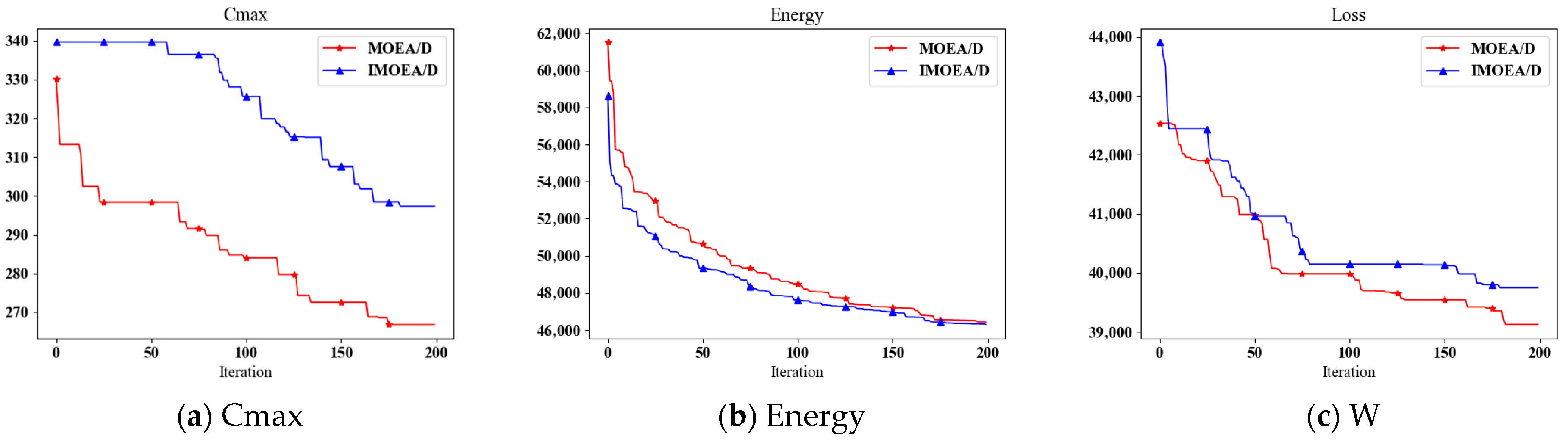
Under the complete rescheduling mode, Figure 1 indicates that introducing operators can significantly enhance the optimization of the energy consumption objective. However, only marginal improvement is observed in tool wear, and no improvement is achieved in terms of the maximum makespan.

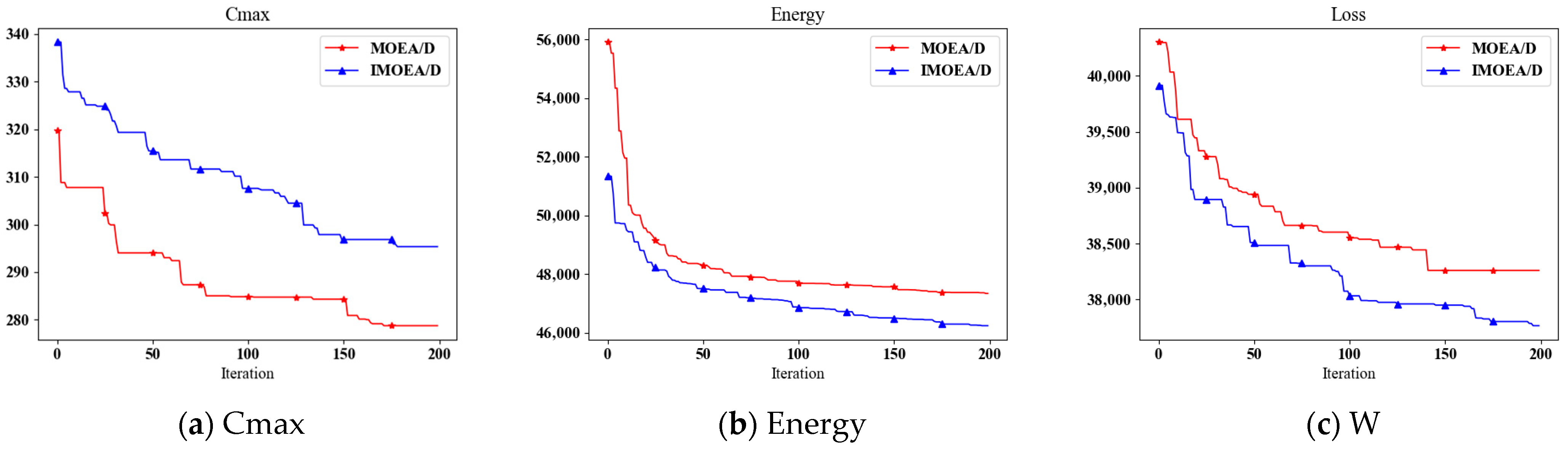
Under the deferred rescheduling (Original Orders First) mode, Figure 2 shows that introducing operators can significantly enhance the optimization of the energy consumption and tool wear objectives. However, no noticeable improvement is obtained for the minimum completion time objective.

Under the deferred rescheduling (Urgents Orders First) mode, Figure 3 indicates that introducing operators can significantly enhance the optimization of the energy consumption and tool wear, whereas the minimum completion time still cannot be effectively improved.

6.2.2. Performance Metric

Compared with MOEA/D, the advantage of IMOEA/D is not reflected in overall convergence quality, but rather in its potential to maintain solution diversity under specific rescheduling scenarios. In particular, under complete rescheduling and deferred rescheduling with urgents processed first, IMOEA/D achieves smaller SPREAD values, indicating a certain superiority in preserving the distribution characteristics of the Pareto solution set. Moreover, IMOEA/D shows relatively smaller fluctuations in HV, suggesting better stability across repeated runs. Therefore, the results indicate that the introduction of operators leads to limited improvement in the overall convergence performance, while it provides a more significant enhancement in preserving the diversity of the Pareto solution set.

Table 5. Performance metrics with and without operators.

		HV	IGD	Spread	Spacing
Complete Rescheduling	MOEA/D	0.4976 ± 0.3261	0.5758 ± 0.1959	0.9123 ± 0.0995	0.0876 ± 0.0768
	IMOEA/D	0.2033 ± 0.1843	0.6148 ± 0.2054	0.7911 ± 0.3166	0.1495 ± 0.1920
Deferred Rescheduling (Original Orders First)	MOEA/D	0.8646 ± 0.4355	0.1827 ± 0.1672	0.8012 ± 0.4530	0.0876 ± 0.0768
	IMOEA/D	0.3040 ± 0.3172	0.8018 ± 0.6097	1.0198 ± 0.0497	0.1495 ± 0.1920
Deferred Rescheduling (Urgents Orders First)	MOEA/D	0.4976 ± 0.3261	0.5758 ± 0.1959	0.9123 ± 0.0995	0.0876 ± 0.0768
	IMOEA/D	0.2033 ± 0.1843	0.6148 ± 0.2054	0.7911 ± 0.3166	0.1495 ± 0.1920

lists the performance metrics under scenarios with and without the proposed operators.

6.2.3. Conclusions

In general, under the three different rescheduling modes, the introduction of operators yields noticeable improvements in the optimization performance of energy consumption and tool wear, while also achieving substantial enhancement in the diversity of the Pareto solution set. These results demonstrate that the introduced operators can effectively strengthen the overall solving capability of the algorithm, particularly in terms of improving solution distribution and optimization quality.

6.3. Scheduling Schemes Comparison

6.3.1. Iterative Evolution of Objective Values Under Different Rescheduling Strategies

Objective values of three different rescheduling methods under the IMOEA/D algorithm. Figure 4 indicates that the complete rescheduling method achieves the poorest overall performance. By comparison, the two deferred rescheduling strategies, Original Orders First and Urgent Orders First, exhibit broadly similar results. Specifically, the urgents-first strategy shows a relative advantage in optimizing the minimum completion time, while the original-first strategy performs better in the optimization of tool wear. This illustrates the target values under three different algorithms. From the comparison, it can be observed that the IMOEA/D algorithm is the optimal one.

6.3.2. Performance Metric

As shown in

Table 6. Comparison of different performance metrics under three rescheduling methods.

	HV	IGD	Spread	Spacing
Complete Rescheduling	0.1776 ± 0.0874	0.8215 ± 0.1194	0.9183 ± 0.1196	0.0588 ± 0.0907
Deferred Rescheduling (Original Orders First)	0.4159 ± 0.4249	0.4289 ± 0.2732	1.0000 ± 0.0348	0.0778 ± 0.0760
Deferred Rescheduling (Urgents Orders First)	0.4558 ± 0.3222	0.5811 ± 0.2817	0.9976 ± 0.0343	0.1301 ± 0.1243

, under the IMOEA/D algorithm, complete rescheduling exhibits the worst overall performance, with the lowest HV and the highest IGD. In contrast, both deferred rescheduling strategies outperform complete rescheduling. Specifically, the urgents-first strategy achieves a higher HV value, indicating better overall optimization quality, whereas the orders-first strategy obtains a lower IGD value and a smaller SPACING value, showing advantages in convergence and solution distribution uniformity. Overall, deferred rescheduling is superior to complete rescheduling, while the two deferred strategies show different strengths.

6.3.3. Conclusions

Overall, the consistent dominance of IMOEA/D across all three policies confirms the effectiveness and general applicability of the proposed approach for tri-objective green rescheduling with urgent order insertion and multi-speed machines. Overall, under the IMOEA/D algorithm, the three rescheduling methods exhibit clear differences in both objective optimization performance and metric-based evaluation results. Among them, complete rescheduling shows the poorest overall performance and does not demonstrate clear advantages in either multi-objective optimization effectiveness or Pareto solution quality. In contrast, both deferred rescheduling strategies achieve better overall results. Specifically, the urgents-first strategy performs better in terms of minimum completion time and overall solution quality, whereas the orders-first strategy shows superior performance in tool wear optimization, convergence, and solution distribution uniformity. For the energy consumption objective, both deferred rescheduling strategies outperform complete rescheduling. In summary, deferred rescheduling is generally more effective than complete rescheduling, although the urgents-first and orders-first strategies differ in their optimization emphasis.

6.4. Algorithms Comparison

6.4.1. Iterative Evolution of Objective Values Under Different Algorithms

As illustrated in Figure 5, Figure 6 and Figure 7, the objective optimization performance of IMOEA/D remains relatively stable under the three different rescheduling strategies, with only minor variations observed. In particular, IMOEA/D consistently performs best in the optimization of energy consumption, demonstrating a clear advantage in this objective. Its performance in tool wear optimization is at a medium level, whereas its optimization effect on the minimum completion time is relatively poor.

6.4.2. Performance Metric

The results in the table indicate that the improvement brought by IMOEA/D is not mainly reflected in absolute superiority in overall convergence performance, but rather in the enhancement of Pareto-solution distribution quality. Although IMOEA/D does not outperform ABC, DE, or the baseline MOEA/D in terms of HV and IGD, it shows certain advantages in diversity- and distribution-related metrics. This suggests that the introduced operators are more effective in improving the structural quality of the solution set than in merely accelerating convergence.

Table 7. Performance metrics under different algorithms.

		HV	IGD	Spread	Spacing
Complete Rescheduling	MOEA/D	0.7168 ± 0.1554	0.3114 ± 0.1263	0.9828 ± 0.0159	0.0126 ± 0.0131
	IMOEA/D	0.5676 ± 0.1774	0.3665 ± 0.1374	0.9482 ± 0.1172	0.0215 ± 0.0336
	NSGA-II	0.1217 ± 0.0752	0.9578 ± 0.1339	0.9066 ± 0.0408	0.0551 ± 0.0220
	INSGA-II	0.1192 ± 0.0541	0.9451 ± 0.1435	0.9654 ± 0.0225	0.0694 ± 0.0264
	ABC	1.0802 ± 0.2293	0.1519 ± 0.1030	0.9899 ± 0.0601	0.0330 ± 0.0187
	DE	0.9569 ± 0.2296	0.2073 ± 0.0994	0.8416 ± 0.2987	0.0451 ± 0.0473
Deferred Rescheduling (Original Orders First)	MOEA/D	0.7808 ± 0.0720	0.2819 ± 0.0662	0.9773 ± 0.0661	0.0369 ± 0.0358
	IMOEA/D	0.5197 ± 0.3464	0.5487 ± 0.3127	0.9978 ± 0.0184	0.0225 ± 0.0244
	NSGA-II	0.0941 ± 0.0494	1.1985 ± 0.3245	0.9602 ± 0.0851	0.0659 ± 0.0406
	INSGA-II	0.1153 ± 0.0287	0.9197 ± 0.1563	0.9853 ± 0.0221	0.1942 ± 0.3176
	ABC	1.1500 ± 0.1801	0.1087 ± 0.0798	0.9381 ± 0.2286	0.0238 ± 0.0222
	DE	0.8532 ± 0.2470	0.2004 ± 0.1146	0.9465 ± 0.0204	0.0121 ± 0.0097
Deferred Rescheduling (Urgents Orders First)	MOEA/D	0.6086 ± 0.2730	0.4131 ± 0.1967	1.0054 ± 0.0329	0.0505 ± 0.0363
	IMOEA/D	0.4346 ± 0.2747	0.6798 ± 0.3110	1.0098 ± 0.0193	0.0610 ± 0.0612
	NSGA-II	0.2046 ± 0.3127	1.1134 ± 0.2002	0.9750 ± 0.0320	0.0517 ± 0.0301
	INSGA-II	0.1041 ± 0.0874	1.0869 ± 0.2440	0.9904 ± 0.0184	0.0834 ± 0.0803
	ABC	1.1847 ± 0.1000	0.1203 ± 0.0967	0.9615 ± 0.2109	0.0259 ± 0.0138
	DE	0.7114 ± 0.3513	0.3635 ± 0.2484	0.9603 ± 0.1165	0.0420 ± 0.0395

summarizes the performance metrics under different algorithms.In this case, IMOEA/D achieves the best SPREAD value (0.9978 ± 0.0184), while its SPACING value (0.0225 ± 0.0244) is clearly better than that of MOEA/D (0.0369 ± 0.0358) and close to those of ABC (0.0238 ± 0.0222) and DE (0.0121 ± 0.0097). This indicates that, under the constraint of preserving the original schedule as much as possible, IMOEA/D can more effectively maintain the range and uniformity of the nondominated solution set, thereby improving the diversity quality of the Pareto front. By contrast, under complete rescheduling and deferred rescheduling with Urgent Orders First, this advantage becomes less pronounced, although the SPREAD values of IMOEA/D remain at a relatively high level, implying that the proposed algorithm still possesses a certain capability for preserving distribution quality under different rescheduling policies.

From a horizontal comparison perspective, IMOEA/D still demonstrates clear advantages over NSGA-II and INSGA-II. Under all three rescheduling modes, IMOEA/D achieves substantially higher HV values and generally lower IGD values than these two algorithms, indicating stronger competitiveness in terms of Pareto-front approximation and overall solution quality. Therefore, although the convergence improvement of IMOEA/D over the original MOEA/D is limited, it still shows better optimization capability than traditional Pareto-based algorithms in multi-objective dynamic rescheduling problems.

Overall, it can be concluded that the main strength of IMOEA/D lies in its enhanced ability to preserve Pareto-solution diversity and distribution quality, especially under deferred rescheduling scenarios. Hence, the introduced operators effectively improve the adaptability and search capability of the algorithm in constrained dynamic rescheduling spaces, making IMOEA/D more suitable for green flexible job shop rescheduling problems that require a balance between solution quality, diversity, and practical implementability.

6.4.3. Conclusions

The comparative results show that different algorithms exhibit distinct characteristics in both objective optimization and metric-based evaluation. IMOEA/D remains relatively stable under the three rescheduling modes and performs best in optimizing energy consumption, while showing moderate performance in tool wear optimization and relatively weak performance in minimum completion time optimization. In terms of performance metrics, ABC generally achieves the best HV and IGD values, followed by DE and MOEA/D. Although IMOEA/D does not demonstrate absolute superiority in overall convergence performance, it performs well in diversity-related metrics. The main strength of IMOEA/D lies in energy optimization and Pareto-solution distribution quality, especially under deferred rescheduling scenarios. Overall, the main strength of IMOEA/D lies in enhancing energy optimization and Pareto-solution distribution, rather than achieving absolute dominance in convergence performance.

7. Conclusions and Future Work

7.1. Conclusions

In conclusion, this paper addresses a tri-objective green flexible job shop rescheduling problem in the presence of urgent order insertion and multi-speed machining. A mathematical model was developed to jointly optimize makespan, total energy consumption, and total tool wear, and two rescheduling strategies—complete rescheduling and deferred rescheduling—were systematically investigated under an event-driven freezing mechanism. To enhance the solution capability in complex dynamic environments, an improved IMOEA/D algorithm with a three-layer encoding scheme was proposed, integrating hybrid initialization, tabu-guided crossover, simulated annealing mutation, and critical-path-based variable neighborhood search. Experimental results demonstrate that the proposed method performs effectively in reducing energy consumption and controlling tool wear, while also improving the diversity and distribution quality of the Pareto solution set. Furthermore, deferred rescheduling generally shows better overall performance than complete rescheduling, whereas the original-orders-first and urgents-first strategies exhibit different strengths in convergence behavior, solution quality, and objective optimization. Overall, this study provides not only an effective modeling and optimization framework for multi-objective green rescheduling problems but also valuable theoretical support and practical guidance for manufacturing systems that seek to balance production efficiency, energy saving, and tool-related cost control.

7.2. Case Study

The proposed method has strong potential for industrial application, especially in flexible manufacturing environments characterized by high-mix low-volume production, frequent urgent-order insertion, and adjustable machine speed levels. In practice, the method can be deployed as a rescheduling module integrated with MES, APS, or digital shop-floor scheduling systems. When an urgent order arrives or another dynamic disturbance occurs, the system can obtain order information, process routes, and due dates from ERP/MES, while real-time machine states, processing progress, and speed-level information can be collected from CNC, PLC, or SCADA systems. Based on the proposed event-driven freezing rule, completed and ongoing operations are fixed, and only the rescheduling window composed of waiting operations and urgent-order operations is re-optimized. Then, IMOEA/D jointly determines operation sequencing, machine assignment, and speed selection, and generates a Pareto solution set with respect to makespan, total energy consumption, and total tool wear. Decision-makers can select a satisfactory solution according to actual production requirements and feed it back to the shop-floor execution layer. Therefore, the proposed method can not only reduce unnecessary disruption to the original production plan and improve implementability but also provide more flexible decision support for balancing production efficiency, energy saving, and tool-related cost control, which demonstrates its practical value in industrial applications.

7.3. Future Work

Future work may be carried out in several directions. First, beyond urgent order insertion, more complex dynamic disturbances such as machine breakdowns, stochastic processing times, material arrival uncertainty, and multiple simultaneous disruptions can be incorporated to improve the adaptability of the model to real manufacturing environments. Second, future studies may integrate shop-floor energy data, equipment monitoring data, and historical tool-wear records to calibrate the model parameters and functional relationships, thereby enhancing model accuracy and industrial applicability. Third, the proposed algorithm can be further extended by introducing adaptive parameter adjustment mechanisms and combining it with machine learning, reinforcement learning, or digital twin technologies to improve its real-time response and intelligent decision-making capability in online rescheduling. Finally, additional criteria such as schedule stability, adjustment cost, start-time deviation, and machine reassignment frequency may be incorporated into the current tri-objective framework, so as to establish a more comprehensive rescheduling model that balances optimization performance with execution feasibility in practical manufacturing systems.

References

1. Sitahong, A.; Wang, G.; Yuan, Y. A Green Flexible Job-shop Scheduling Model for Multiple AGVs Considering Carbon Footprint. Energy-Efficient Scheduling in Dynamic Flexible Job Shops: A Review. Sustainability 2025, 17, 11009. [Google Scholar] [CrossRef]
2. Ren, F.; Liu, H. Dynamic scheduling for flexible job shop based on MachineRank algorithm and reinforcement learning. Sci. Rep. 2024, 14, 29741. [Google Scholar] [CrossRef] [PubMed]
3. Wang, Z.; He, M.; Wu, J.; Chen, H.; Cao, Y. An improved MOEA/D for low-carbon many-objective flexible job shop scheduling problem. Comput. Ind. Eng. 2024, 188, 109926. [Google Scholar] [CrossRef]
4. Ding, J.; Chen, M.; Wang, T. A Survey of AI-enabled Dynamic Manufacturing Scheduling: From Directed Heuristics to Autonomous Learning. ACM Comput. Surv. 2023, 55, 307. [Google Scholar] [CrossRef]
5. Gao, Q.; Liu, J.; Li, H. Digital twin-driven dynamic scheduling for the assembly workshop of complex products with workers allocation. Robot. Comput. Integr. Manuf. 2024, 89, 102786. [Google Scholar] [CrossRef]
6. Wang, J.; Li, R.; Wang, Q. Optimization of Dynamic Scheduling for Flexible Job Shops Using Multi-Agent Deep Reinforcement Learning. Processes 2025, 13, 4045. [Google Scholar] [CrossRef]
7. Duan, J.; Wang, J. Energy-efficient scheduling for a flexible job shop with machine breakdowns considering machine idle time arrangement and machine speed level selection. Comput. Ind. Eng. 2021, 161, 107667. [Google Scholar] [CrossRef]
8. Wang, J.; Wu, C.; Peng, Y. Multi-objective scheduling for an energy-efficient flexible job shop problem with peak power constraint. Appl. Soft Comput. 2024, 167, 112330. [Google Scholar] [CrossRef]
9. Tian, Y.; Gao, Z.; Zhang, L.; Chen, Y. A Multi-Objective Optimization Method for Flexible Job Shop Scheduling Considering Cutting-Tool Degradation With Energy-Saving Measures. Mathematics 2023, 11, 324. [Google Scholar] [CrossRef]
10. Albayrak, C.; Önüt, S. Energy-efficient scheduling for a flexible job shop problem considering rework processes and new job arrival. Int. J. Ind. Eng. Comput. 2024, 15, 871–886. [Google Scholar] [CrossRef]
11. Naimi, R.; Nouiri, M.; Cardin, O. A Q-Learning Rescheduling Approach to the Flexible Job Shop Problem Combining Energy and Productivity Objectives. Sustainability 2021, 13, 13016. [Google Scholar] [CrossRef]
12. Luo, J.; Yi, S.; Lin, Z. Petri-net-based deep reinforcement learning for real-time scheduling of automated manufacturing systems. J. Manuf. Syst. 2024, 74, 995–1008. [Google Scholar] [CrossRef]
13. Shen, L.; Dauzère-Pérès, S. Energy cost efficient scheduling in flexible job-shop manufacturing systems. Eur. J. Oper. Res. 2023, 310, 992–1016. [Google Scholar] [CrossRef]
14. Salama, M.; Srinivas, S. Adaptive neighborhood simulated annealing for sustainability-oriented single machine scheduling with deterioration effect. Appl. Soft Comput. 2021, 110, 107632. [Google Scholar] [CrossRef]
15. Grassi, A.; Guizzi, G. A Genetic-Algorithm-Based Approach for Optimizing Tool Utilization and Makespan in FMS Scheduling. J. Manuf. Mater. Process. 2023, 7, 75. [Google Scholar] [CrossRef]
16. Hwangbo, S.; Liu, J.J.; Ryu, J.-H. Production rescheduling via explorative reinforcement learning while considering nervousness. Comput. Chem. Eng. 2024, 186, 108700. [Google Scholar] [CrossRef]
17. Lv, L.; Zhang, C.; Fan, J.; Shen, W. Deep reinforcement learning for job shop scheduling problems: A comprehensive literature review. Knowl.-Based Syst. 2025, 321, 113633. [Google Scholar] [CrossRef]
18. Zhang, C.; Zhu, G.-Y. A literature review of reinforcement learning methods applied to job-shop scheduling problems. Comput. Oper. Res. 2025, 175, 106929. [Google Scholar] [CrossRef]
19. Dauzère-Pérès, S.; Ding, J. The flexible job shop scheduling problem: A review. Eur. J. Oper. Res. 2024, 314, 409–432. [Google Scholar] [CrossRef]
20. Meng, L.; Zhang, C.; Zhang, B. MILP modeling and optimization of multi-objective flexible job shop scheduling problem with controllable processing times. Swarm Evol. Comput. 2023, 82, 101374. [Google Scholar] [CrossRef]
21. Qu, H.; Tong, X.; Cai, M. Energy-saving scheduling strategy for variable-speed flexible job-shop problem considering operation-dependent energy consumption. Expert Syst. Appl. 2024, 256, 124952. [Google Scholar] [CrossRef]
22. Wen, X.; Lian, X.; Qian, Y. Dynamic scheduling method for integrated process planning and scheduling problem with machine fault. Robot. Comput. Integr. Manuf. 2022, 77, 102334. [Google Scholar] [CrossRef]
23. Chen, R.; Cheng, T.C.E.; Ng, C.T. Rescheduling to trade off between global disruption of original jobs with flexibility and scheduling cost of new jobs. Omega 2024, 128, 103114. [Google Scholar] [CrossRef]
24. Song, J.; Shen, Y.; Wang, L. An Efficient Job Insertion Algorithm for Hybrid Human–Machine Collaborative Flexible Job Shop Scheduling with Random Job Arrivals. Electronics 2025, 14, 3397. [Google Scholar] [CrossRef]
25. Lu, D.; Gong, G.; Gong, Z. A distributed flexible job shop scheduling problem considering rush order insertion using a two-stage memetic algorithm. Appl. Soft Comput. 2026, 186, 114008. [Google Scholar] [CrossRef]
26. Xiao, B.; Zhao, Z.; Wu, Y. An improved MOEA/D for multi-objective flexible job shop scheduling by considering efficiency and cost. Comput. Oper. Res. 2024, 167, 106674. [Google Scholar] [CrossRef]
27. Han, X.; Cheng, W.; Meng, L. A dual population collaborative genetic algorithm for solving flexible job shop scheduling problem with AGV. Swarm Evol. Comput. 2024, 86, 101538. [Google Scholar] [CrossRef]
28. Liu, L.; Guo, K. Digital Twin-Driven Adaptive Scheduling for Flexible Job Shops. Sustainability 2022, 14, 5340. [Google Scholar] [CrossRef]
29. Yin, L.; Gao, Q. Research on Multi-Objective Flexible Job Shop Scheduling Optimization Based on Improved Salp Swarm Algorithm in Rolling Production Mode. Appl. Sci 2025, 15, 5947. [Google Scholar] [CrossRef]
30. Xie, J.; Gao, L.; Li, X.; Gui, L. A hybrid genetic tabu search algorithm for distributed job-shop scheduling problems. Swarm Evol. Comput. 2024, 90, 101670. [Google Scholar] [CrossRef]
Figure 1. Comparative Results of Algorithms under Complete Rescheduling.
Designs 10 00041 g001
Figure 2. Comparative Results of Algorithms under Deferred Rescheduling (Original Orders First).
Designs 10 00041 g002
Figure 3. Comparative Results of Algorithms under Deferred Rescheduling (OriginalOrders First).
Designs 10 00041 g003
Figure 4. Comparative Results of Scheduling Schemes.
Designs 10 00041 g004
Figure 5. Comparative Results of Algorithms under Complete Rescheduling.
Designs 10 00041 g005
Figure 6. Comparative Results of Algorithms under Deferred Rescheduling (Original Orders First).
Designs 10 00041 g006
Figure 7. Comparative Results of Algorithms under Deferred Rescheduling (Urgent Orders First).
Designs 10 00041 g007