Simulation-Driven Screening and Machine Learning Surrogate Modelling of Water Pipeline Start-Up and Filling Operations for Engineering Design Support

Abstract

Filling operations in pressurised pipeline systems can trap air pockets, generating hazardous transient overpressures that threaten structural integrity and operational reliability. Evaluating these events using conventional hydraulic models can be computationally intensive, limiting design-space exploration of operational scenarios. This study presents a simulation-driven design-screening framework based on Monte Carlo simulation to evaluate and predict peak absolute pressures during pipeline start-up and filling operations. A total of 2000 transient scenarios were generated for a representative 1100 m pipeline system by varying key geometric and operational parameters, including diameter, friction factor, column lengths, slopes, and reservoir elevation. Twenty-eight machine learning regression models were trained to develop a physics-informed surrogate model capable of rapidly predicting pressure peaks within the defined parameter domain. The trilayered neural network achieved the highest predictive accuracy, with robust validation (RMSE = 10.95 m, R² = 0.99) and test performance (RMSE = 9.78 m, R² = 0.99). Screening results showed that nominal pressure thresholds of 61.18 m and 407.89 m were exceeded in 97.53% and 4.89% of the retained peak-forming scenarios (n = 1746), respectively. The proposed framework provides an efficient and reproducible surrogate-based design-screening approach for transient overpressure risk within the evaluated hydraulic domain.

1. Introduction

Within pressurised conveyance systems, commissioning and pipeline filling operations are routine activities that can induce rapid pressure fluctuations and increase the risk of damage to the pipe and its components, particularly under conditions of limited control [1,2,3,4,5]. In urban and industrial settings, such phenomena may compromise the system’s structural integrity and service continuity [6,7]. Consequently, a detailed analysis of hydraulic transients is essential to ensure adequate performance and to prevent failures caused by overpressure or structural collapse [8,9,10].

Predicting pressure peaks becomes more challenging when entrapped air is present within the pipeline, leading to highly nonlinear flow behaviour [11,12,13]. During filling, air pockets may compress and expand, generating oscillations and significant transient pressure surges [14,15,16,17]. The magnitude of these peaks depends on the system geometry, pipe slope, valve locations, and the volume of entrapped air [18,19,20,21,22]. These factors highlight the need for robust, efficient methods that can rapidly assess critical conditions, thereby improving operational decision-making and reducing field risks [23,24].

A range of hydraulic modelling approaches has been developed to analyse transient phenomena. Rigid column models provide rapid estimates by simplifying the system, and are therefore helpful for preliminary assessments where pipe deformation need not be represented [25,26]. However, elastic models, which account for water compressibility and pipe-wall deformation, enable a more realistic representation of pressure-wave propagation, albeit with increased complexity and computational cost [27,28]. In parallel, one-dimensional (1D) models based on the Method of Characteristics are widely used in engineering to simulate the time-dependent evolution of flow and pressure [29,30]. Conversely, two- or three-dimensional CFD (Computational Fluid Dynamics) models have become established as high-fidelity tools for investigating air–water interactions and flow structures during filling or emptying processes [31,32,33,34]. Nevertheless, their use in parametric studies is constrained by sensitivity to boundary conditions, model setup requirements, and high computational expense [35].

In response to these limitations, machine learning (ML) approaches have been explored for the rapid and accurate prediction of pressure peaks [36]. This strategy reframes a complex transient hydraulic problem as a supervised prediction task by generating a dataset that links operational conditions to recorded maximum pressures [37,38,39]. Once trained, an ML model can estimate the pressure peak under new operating conditions without running a full hydraulic simulation, thereby substantially reducing analysis time [40,41,42]. MATLAB provides 28 regression model configurations, including linear regression, decision trees, support vector machines (SVM), Gaussian Process Regression (GPR), ensemble methods, and neural networks, enabling systematic comparison of alternative surrogate modelling approaches [43]. This comprehensive selection was chosen to rigorously compare diverse algorithms, ensuring the identification of the most robust and accurate model capable of capturing the severe non-linearities of rapid pipe filling operations.

Recent studies have demonstrated the growing applicability of machine learning methods for predicting hydraulic transient behaviour and pressure surges in pipeline systems. Artificial neural networks and hybrid physics–ML approaches have been successfully applied to estimate transient pressure responses and accelerate computational workflows traditionally based on numerical simulation. For example, neural network models have shown strong predictive performance in modelling water hammer and transient flow dynamics, providing rapid surrogate predictions whilst preserving physical interpretability [44]. Similarly, uncertainty quantification and sensitivity analysis studies have highlighted the feasibility of combining stochastic sampling and data-driven methods to characterise transient pressure amplification mechanisms in pressurised systems [45]. More recently, hybrid physics-informed machine learning frameworks have demonstrated improved predictive stability and generalisation when applied to hydraulic transient phenomena [46]. These developments confirm the potential of machine learning as a surrogate modelling tool for accelerating transient pressure evaluation. However, existing studies have primarily focused on isolated transient events or network-scale pressure estimation, whereas the present work integrates Monte Carlo-based screening with physics-informed surrogate modelling to systematically evaluate air-pocket-induced pressure peaks within a physically constrained parameter domain.

In this study, a training procedure was implemented using a Monte Carlo approach to define the ranges of the input variables describing the filling manoeuvre, system geometry, and operating conditions [47]. A dataset was generated from hydraulic simulations using MATLAB’s Sensitivity Analyzer App [48]. To ensure representative coverage of the input space, uniform random sampling was used, and the maximum pressure from each simulation was used as the target variable. Subsequently, 28 regression models (neural networks, decision trees, and ensemble methods) were trained, and their performance was assessed using error metrics and predictive capability indicators [35]. The results showed that a three-layer artificial neural network achieved the best overall performance, with high accuracy and stability across both the validation and test datasets. This model enables efficient prediction of pressure peaks and serves as a practical tool to support operational decision-making, enhance the system’s hydraulic safety, and reduce risks during commissioning, filling, and routine operation.

This investigation proposes a simulation-driven screening framework to evaluate transient overpressures during pipeline start-up and filling operations with entrapped air, integrating physics-based modelling and machine learning to overcome the computational cost and technical complexity associated with CFD, numerical, and analytical transient solutions in environments such as Simulink-MATLAB R2025a. In this context, the objective is to analyse pipeline start-up processes by combining a rigid column mathematical model with machine learning regression to transform a complex physical problem into an efficient predictive and screening tool within the defined parameter domain. Methodologically, a system of differential equations is formulated and solved numerically to compute the governing hydraulic and thermodynamic variables. Subsequently, a structured sensitivity analysis is conducted using Monte Carlo sampling with the Sensitivity Analyzer App to generate a representative dataset for training, validation, and testing. Finally, machine learning regression models are applied to develop a physics-informed surrogate model capable of rapidly predicting maximum pressure peaks, enabling efficient scenario screening and supporting risk-informed operational assessment, whilst remaining consistent with established transient hydraulic modelling principles. From an engineering design perspective, this workflow enables reproducible design-space screening to support the selection of start-up control strategies and ISO PN class constraints during pipeline design and commissioning.

2. Materials and Methods

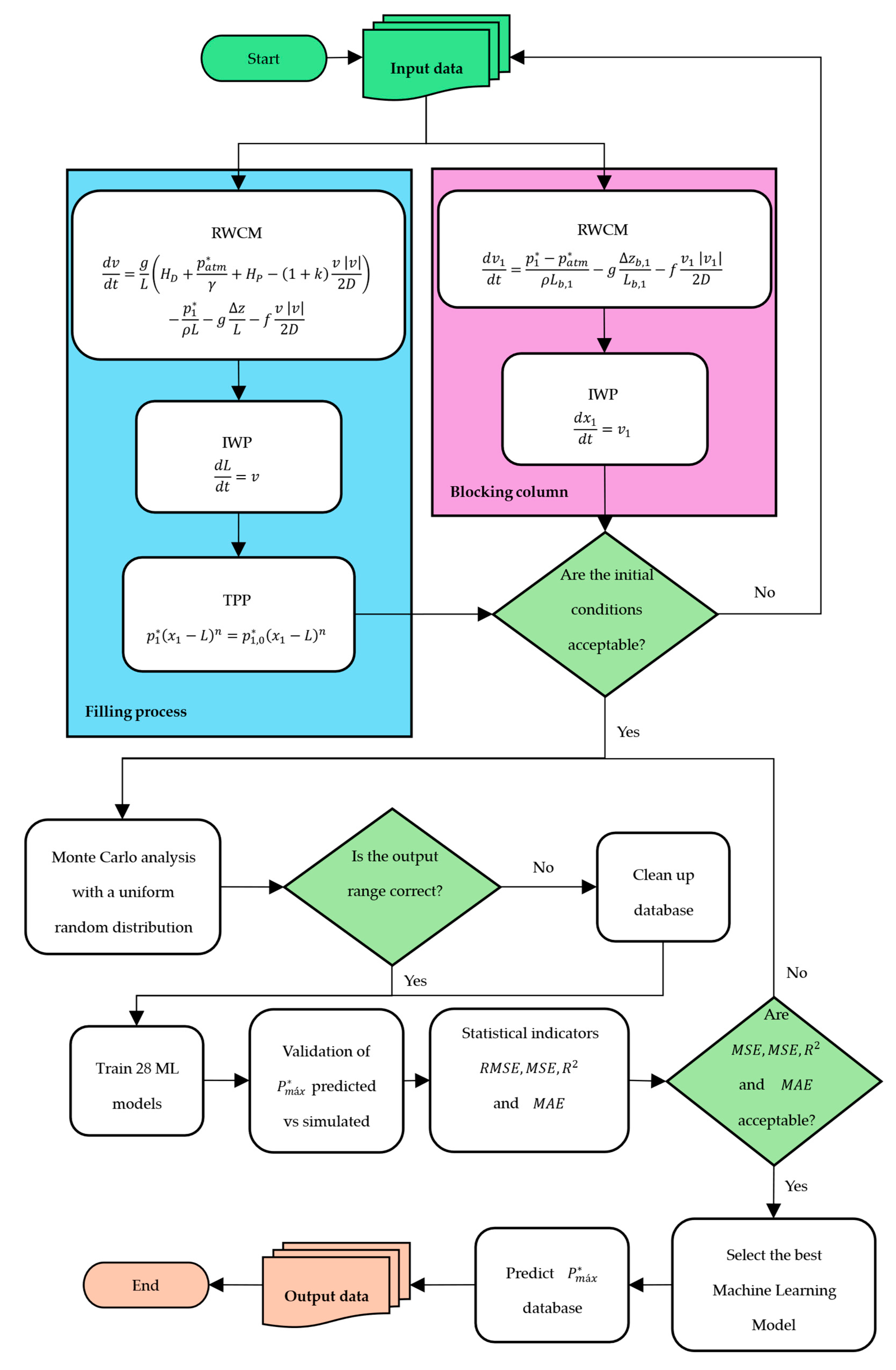
Figure 1 summarises the workflow, combining the rigid water column model, Monte Carlo scenario generation, and machine learning regression. First, the filling column, entrapped air pocket, and blocking column are simulated using the rigid column formulation (Section 2.1). Second, physically admissible ranges are defined for the input parameters and used in a sensitivity/Monte Carlo analysis to generate the training dataset (Section 2.2). Third, the 28 regression models available in MATLAB Regression Learner (Section 2.3) are trained and evaluated using validation and test statistics to identify the most accurate surrogate. Finally, the selected model is exported, applied to the case study, and compared with the hydraulic simulation response.

2.1. Rigid Water Column Model

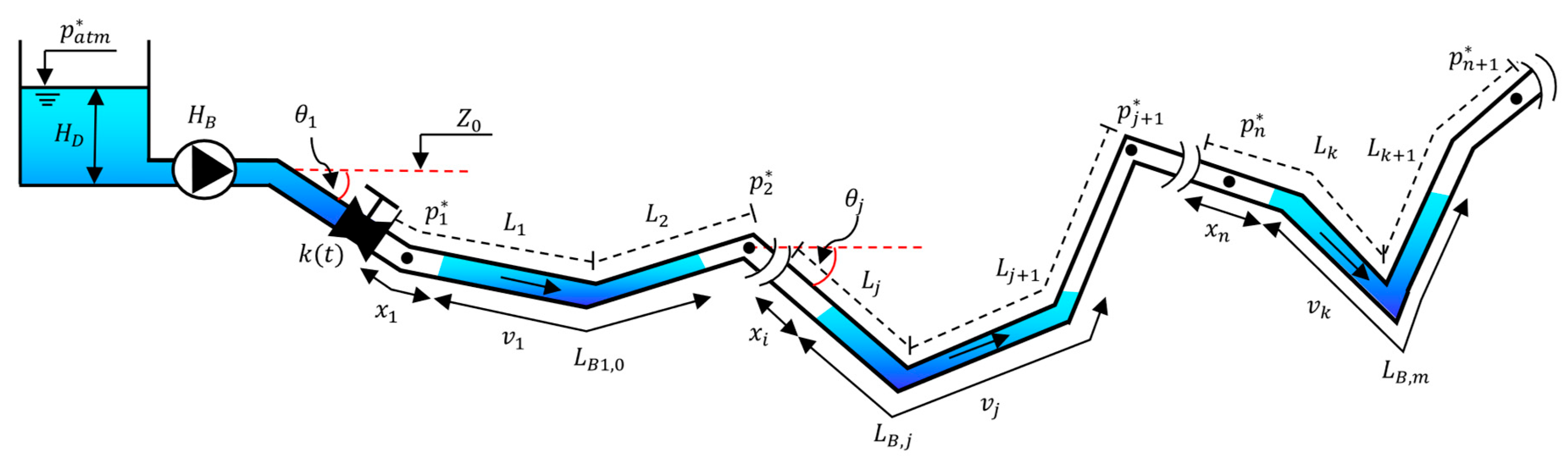
In this section, the schematic configuration shown in Figure 2 is adopted, in which the conduit exhibits a non-uniform alignment composed of pipe branches with constant slopes and contains $n$ trapped air pockets. At the upstream end, an energy-supplying device (tank and/or pump) is installed, and at the outlet, a valve is provided to control discharge. The initial liquid column, of length ($L_0$), is driven by this energy source and begins to propagate into the pipe once the discharge valve is opened, thereby compressing the air located immediately downstream of the valve. The assemblage comprising the energy source, the discharge valve, and the initial filling column defines the boundary condition at the upstream end of the system.

This section presents the mathematical model for simulating the behaviour of the filling process of pipes with diameter $D$ and slopes ${\theta }_1, {\theta }_2, {\theta }_3,\dots , { \theta }_j$, supplied by a storage tank with water depth $H_D$, connected to a pump with characteristic curve $H_P=A_P-C_P{Q}^2$, where $A_P$ and $C_P$ are coefficients of the pump curve, with a control valve with dimensionless loss coefficients $k$, without purge or air valves, and a single blocking water column with length $L_{B1,0}$, to determine the pressure $p_1^{*}$ at the air phase in the pipeline. To analyse the behaviour of overpressures, the rigid column model is employed, which has been validated by various authors, taking into account the inclusion of trapped air pockets and blocking columns [49,50].

The equations are described in general terms below:

• Equation of a filling column using the rigid column model:

$${\displaystyle \frac{dv}{dt}}={\displaystyle \frac{g}{L}}\left(H_D+{\displaystyle \frac{p_{atm}^{*}}{\gamma }}+H_P-\left(1+k\right){\displaystyle \frac{v \left|v\right|}{2D}}\right)-{\displaystyle \frac{p_1^{*}}{\rho L}}-g{\displaystyle \frac{∆z}{L}}-f{\displaystyle \frac{v \left|v\right|}{2D}}$$

(1)

• Equation for the position of a filling column:

$${\displaystyle \frac{dL}{dt}}=v$$

(2)

• Equation of a blocking column $i (i=1, 2, 3,\dots ,m)$ using the rigid column model:

$${\displaystyle \frac{d{v}_j}{dt}}={\displaystyle \frac{p_j^{*}-p_{j+1}^{*}}{\rho L_{b,j}}}-g{\displaystyle \frac{∆z_{b,j}}{L_{b,j}}}-f{\displaystyle \frac{v_j \left|v_j\right|}{2D}}$$

(3)

• Equation of an air-pocket evolution:

$$p_1^{*}{\left(x_1-L_{B1,0}\right)}^n=p_{j,0}^{*}{\left(x_i-L_{B,j}\right)}^n=const.$$

(4)

• Equation for the position of a blocking column:

$${\displaystyle \frac{d{x}_j}{dt}}=v_j$$

(5)

2.2. Sensitivity Analysis

In this section, the model used to analyse the filling process in two pipelines supplied by a tank or a pump is presented, accounting for an air pocket that is compressed during filling and a water column blockage at the lower break. Subsequently, the governing equations required to analyse the proposed model are formulated.

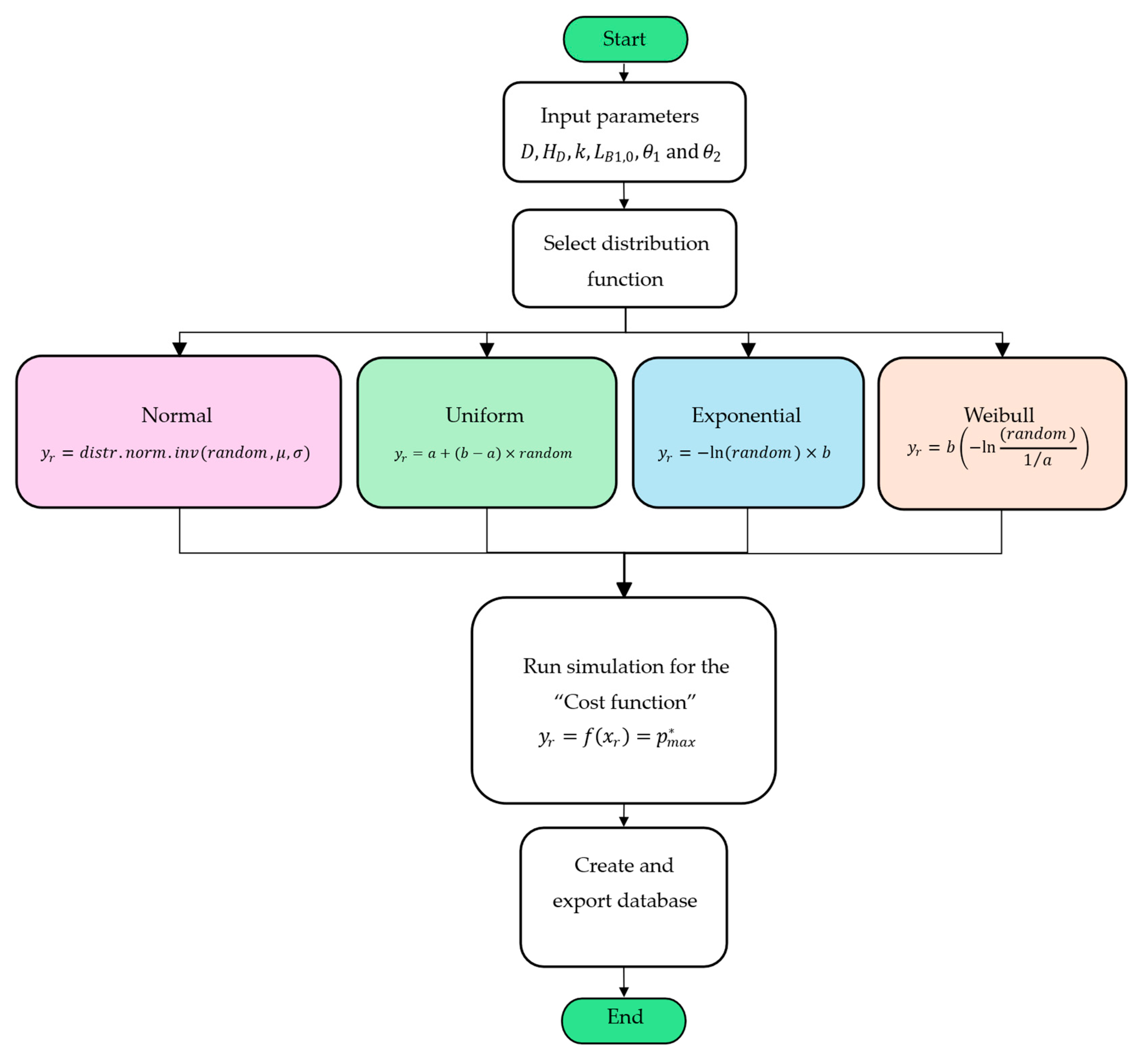
To simulate the results, the sensitivity analysis tool in the Control System Toolbox in MATLAB Simulink was used to automatically generate 2000 simulations using the methodology described in Figure 3. All Monte Carlo sampling and subsequent dataset partitioning were executed under a fixed random generator state (rng(42,’twister’)) set prior to both scenario generation and the train/validation/test splitting procedure to ensure that the same scenarios and splits can be reproduced.

All input parameters were sampled from independent uniform probability distributions within physically constrained bounds to ensure unbiased, space-filling exploration of the admissible transient-response domain. Uniform sampling avoids imposing assumptions on the likelihood of specific operating conditions and is appropriate for screening and surrogate training, where the goal is to characterise the response surface and identify critical combinations rather than estimate operational frequency distributions. Accordingly, alternative prior distributions (e.g., triangular or truncated normal centred on typical operation) were not evaluated, and all exceedance percentages are interpreted as conditional screening metrics under uniform sampling within the defined bounds.

2.3. Design-Space Definition and Screening Criteria Based in Machine Learning Regression Models

In engineering terms, the definition of the admissible design space for start-up transients, while the Monte Carlo procedure provides a space-filling screening strategy to explore feasible combinations of geometric and operational factors. Scenarios are screened to retain only peak-forming cases consistent with the target phenomenon (air-pocket compression-induced pressure peaks), and these retained cases form the basis for surrogate training and exceedance-based design checks against ISO nominal pressure (PN) classes. This structure supports rapid design-space exploration and the identification of governing factors and critical manoeuvres within the defined bounds.

2.4. Machine Learning Regression Models

With the results obtained from the iterations in the database, regression was performed using the Regression Learner application from MATLAB’s Statistics and Machine Learning Toolbox package, where $D$, $H_D$, $k$, $L_{B1,0}$, ${\theta }_1$ and ${\theta }_2$ were entered as predictors. The 28 available regression models (see

Table 1. Machine learning regression models.

Model	Subtypes
Linear Regression	Linear, Interactions Linear, Robust Linear, Stepwise Linear
Tree	Fine Tree, Medium Tree, Coarse Tree
Support Vector Machine (SVM)	Linear SVM, Quadratic SVM, Cubic SVM, Fine Gaussian SVM, Medium Gaussian SVM, Coarse Gaussian SVM
Gaussian Process Regression (GPR)	Squared Exponential GPR, Matern 5/2 GPR, Exponential GPR, Rational Quadratic GPR
Ensemble	Boosted Trees, Bagged Trees
Neural Network	Narrow Neural Network, Medium Neural Network, Wide Neural Network, Bilayer Neural Network, Trilayer Neural Network
Efficient Linear	Efficient Linear Least Squares, Efficient Linear SVM
Kernel	Least Squares Regression Kernel, SVM Kernel

Note: The toolbox presented in Reference [43] was employed in this research.

) were evaluated using RMSE, MSE, R², and MAE, where the regression target variable corresponds to the maximum absolute air-pocket pressure peak obtained during each simulated pipeline start-up transient.

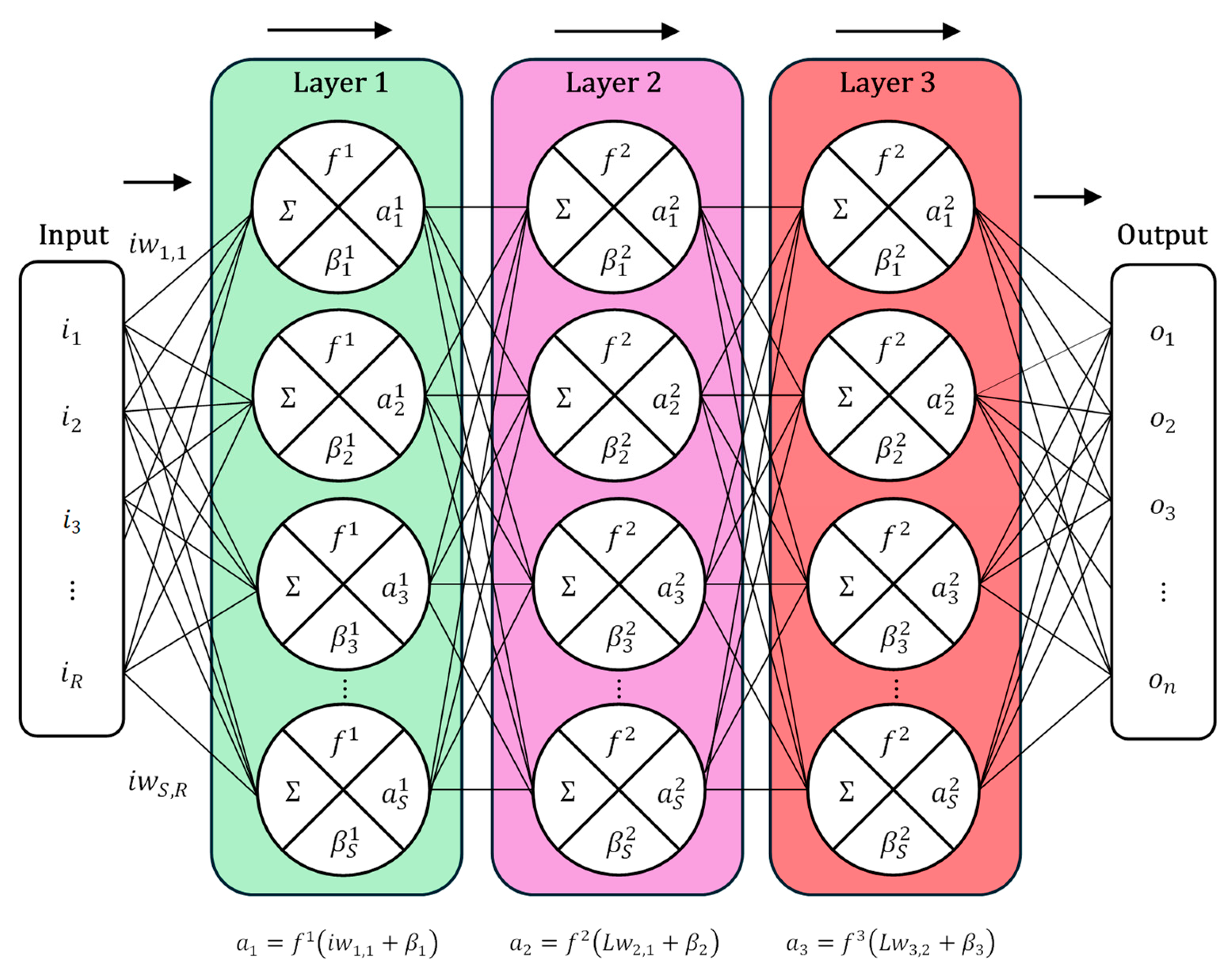
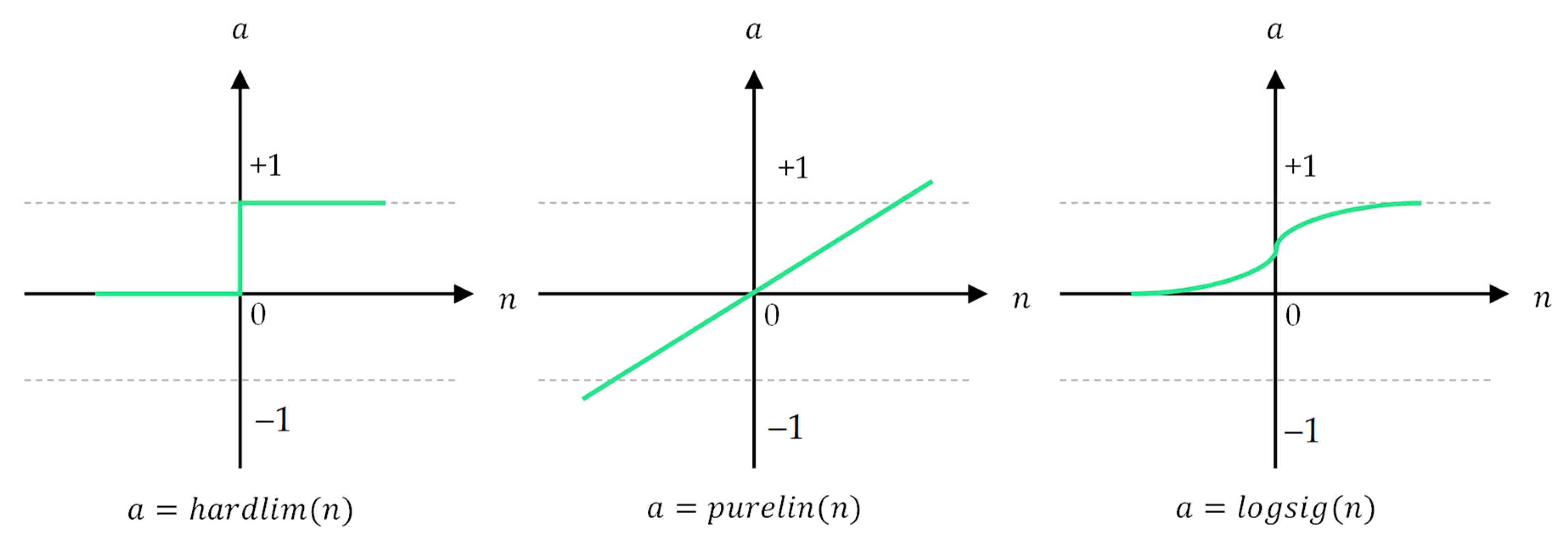
Based on the validation and test statistics, the trilayered neural network was selected as the best surrogate for predicting peak pressures during pipeline filling with entrapped air. Figure 4 shows the adopted architecture, which maps the input predictor vector through three hidden layers (with bias terms and transfer functions) to the output peak pressure. The transfer functions considered (Hardlim, Purelin, and Logsig) are shown in Figure 5.

$$\overrightarrow{i}=\left[\begin{array}{c}{i}_1\\ i_2\\ \begin{array}{c}{i}_3\\ ⋮\\ i_5\end{array}\end{array}\right]$$

(6)

$$\overrightarrow{W}=\left[\begin{array}{ccccc}{w}_{1,1}& w_{1,2}& w_{1,3}& \dots & w_{1,R}\\ w_{2,1}& w_{2,2}& w_{2,3}& \dots & w_{2,R}\\ w_{3,1}& w_{3,2}& w_{3,3}& \dots & w_{3,R}\\ ⋮& ⋮& ⋮& \dots & ⋮\\ w_{S,1}& w_{S,2}& w_{S,3}& \dots & w_{S,R}\end{array}\right]$$

(7)

$$i{w}_{S,R}=\overrightarrow{W}\times \overrightarrow{i}$$

(8)

$$n=\sum \overrightarrow{W}\times \overrightarrow{i}+\overrightarrow{\beta }$$

(9)

$$a^3=f^3\left(L{w}_{\mathrm{3,2}}\mathsf{\bullet }{f}^2\left(L{w}_{\mathrm{2,1}}\mathsf{\bullet }{f}^1\left(i{w}_{\mathrm{1,1}}+{\beta }_1\right) \right)+{\beta }_2\right)+{\beta }_3$$

(10)

Table 2. Regression indicators.

Indicator	Formula	Equation No.
Mean Squared Error	$MSE={\displaystyle \frac{\sum {\left(y-\widehat{y}\right)}^2}{n}}$	(11)
Root Mean Squared Error	$RMSE=\sqrt{{\displaystyle \frac{\sum {\left|y-\widehat{y}\right|}^2}{n}}}$	(12)
R-Squared	$R^2=1-{\displaystyle \frac{\sum {\left(y-\widehat{y}\right)}^2}{\sum {\left(y-\overline{y}\right)}^2}}$	(13)
Mean Absolute Error	$MAE={\displaystyle \frac{\sum {\left|y-\widehat{y}\right|}^2}{n}}$	(14)

summarises the error metrics used to evaluate the regression models. MSE penalises large errors quadratically and is aligned with squared-loss optimisation. RMSE is the square root of MSE, reported in the same units as the predicted peak pressure and is therefore easier to interpret as a typical error magnitude. MAE uses absolute deviations, making it less sensitive to outliers than quadratic metrics. R² measures the fraction of variance explained relative to a mean predictor and is most informative when reported alongside error-magnitude metrics (RMSE/MAE).

All regression models were trained using the predefined configurations available in MATLAB Regression Learner. The corresponding hyperparameters and model settings are reported in Appendix A (

Table A1. Hyperparameters.

Model Type	Model	Hyperparameters	Prediction Speed (obs/s)	Training Time (s)
Linear Regression	Linear	Terms: Linear	317,414.51	3.97
Linear Regression	Robust Linear	Terms: Linear Robust fitting: Enabled	260,833.48	3.90
Linear Regression	Interactions Linear	Terms: Linear + Interactions	180,187.56	5.76
Stepwise Regression	Stepwise Linear	Initial terms: Linear Maximum terms: Interactions	250,512.41	3.63
Decision Tree	Fine Tree	Minimum leaf size: 4	200,181.98	3.60
Decision Tree	Medium Tree	Minimum leaf size: 12	349,234.07	3.53
Decision Tree	Coarse Tree	Minimum leaf size: 36	251,759.46	3.51
Support Vector Machine	Linear SVM	Kernel function: Linear	268,031.19	15.18
Support Vector Machine	Quadratic SVM	Kernel function: Quadratic	187,833.51	2.87
Support Vector Machine	Cubic SVM	Kernel function: Cubic	238,366.11	3.76
Support Vector Machine	Fine Gaussian SVM	Kernel function: Gaussian Kernel scale: 0.61	184,928.34	3.73
Support Vector Machine	Medium Gaussian SVM	Kernel function: Gaussian Kernel scale: 2.4	237,580.99	3.68
Support Vector Machine	Coarse Gaussian SVM	Kernel function: Gaussian Kernel scale: 9.8	206,766.92	3.77
Ensemble	Bagged Trees	Number of learners: 30 Minimum leaf size: 8	58,237.26	3.88
Ensemble	Boosted Trees	Number of learners: 30 Minimum leaf size: 8 Learning rate: 0.1	99,750.62	3.62
Gaussian Process Regression	Squared Exponential GPR	Kernel function: Squared Exponential	67,903.33	13.60
Gaussian Process Regression	Matern 5/2 GPR	Kernel function: Matern 5/2	40,559.72	16.37
Gaussian Process Regression	Rational Quadratic GPR	Kernel function: Rational Quadratic	53,779.87	32.78
Gaussian Process Regression	Exponential GPR	Kernel function: Exponential	53,045.92	19.69
Neural Network	Narrow Neural Network	Hidden layers: 1 Neurons per layer: 10	129,145.88	6.64
Neural Network	Medium Neural Network	Hidden layers: 1 Neurons per layer: 25	145,531.52	8.58
Neural Network	Wide Neural Network	Hidden layers: 1 Neurons per layer: 100	291,622.48	8.49
Neural Network	Bilayered Neural Network	Hidden layers: 2 Neurons per layer: 10	193,194.29	6.43
Neural Network	Trilayered Neural Network	Hidden layers: 3 Neurons per layer: 10	314,263.27	4.49
Kernel Regression	Least Squares Regression Kernel	Learner: Least Squares	123,287.29	4.00
Kernel Regression	SVM Kernel	Learner: SVM	145,608.58	4.74
Efficient Linear Model	Efficient Linear Least Squares	Learner: Least Squares	216,269.35	4.43
Efficient Linear Model	Efficient Linear SVM	Learner: SVM	295,302.01	3.44

), ensuring reproducibility and transparency of the surrogate model training procedure.

3. Results

3.1. Hydraulic Modelling

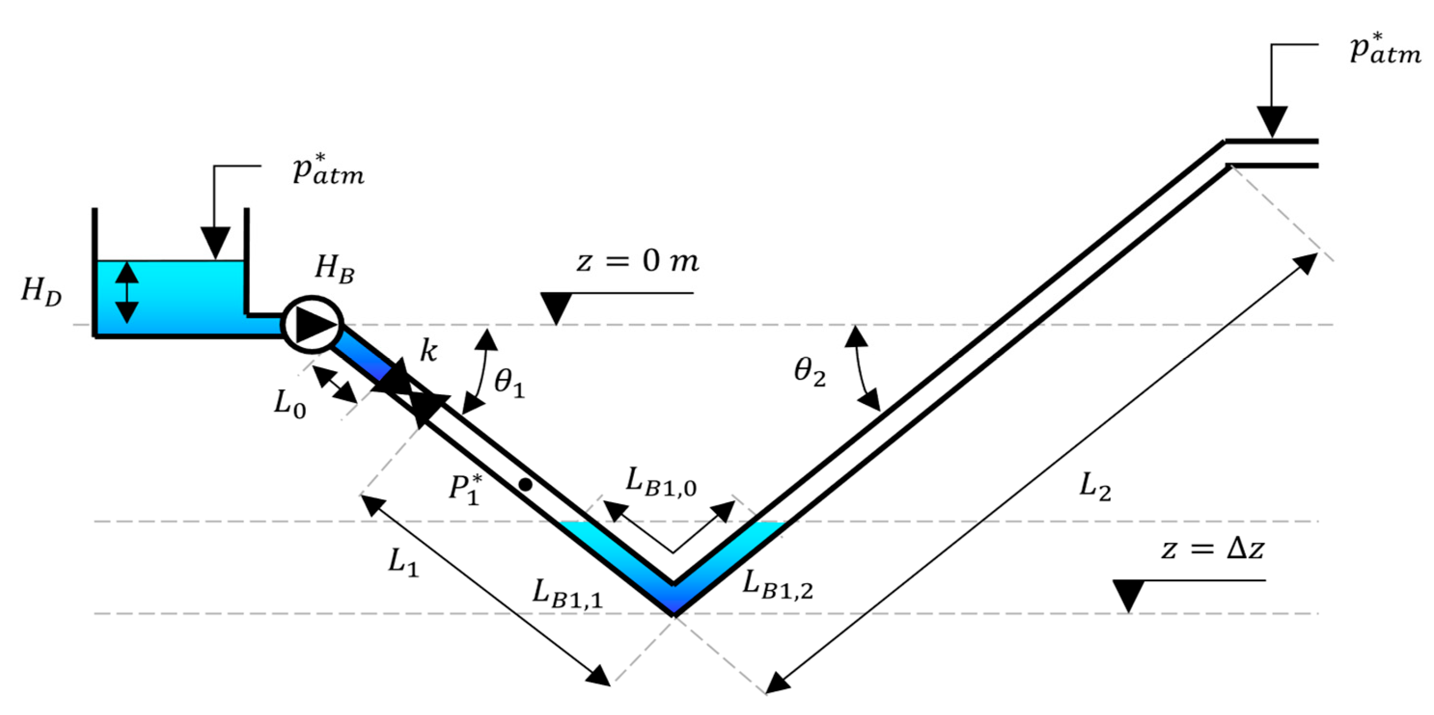
This section presents the mathematical model for simulating the behaviour of the filling process of two pipes of diameter $D=0.30\mathrm{ m}$ and longitudinal slopes ${\theta }_1=15°$ and ${\theta }_2=15°$, supplied by a storage tank with water depth $H_D=4 \mathrm{m}$, connected to a pump with characteristic curve $H_P=A_P-C_P{Q}^2$ where $A_P=150$ and $C_P=80$, with a control valve with dimensionless loss coefficients $k= 0.2,1.15, 5.6$ and 24 for cases of full, ${\displaystyle \raisebox{1ex}{$3$}\!\left/ \!\raisebox{-1ex}{$4$}\right.}$, ${\displaystyle \raisebox{1ex}{$1$}\!\left/ \!\raisebox{-1ex}{$2$}\right.}$, and ${\displaystyle \raisebox{1ex}{$1$}\!\left/ \!\raisebox{-1ex}{$4$}\right.}$ aperture, without an air valve, and a one blocking water column with length $L_{B1,0}$, to determine the pressure $p_1^{\mathrm{*}}$ at the air phase in the pipeline [5,12]. Figure 6 presents the schematic representation of the analysed filling procedure.

The following equations govern the system:

• Equation of the filling column using the rigid model:

$${\displaystyle \frac{dv}{dt}}={\displaystyle \frac{g}{L}}\left(H_D+{\displaystyle \frac{p_{atm}^{*}}{\gamma }}+H_P-\left(1+k\right){\displaystyle \frac{v \left|v\right|}{2D}}\right)-{\displaystyle \frac{p_1^{*}}{\rho L}}-g{\displaystyle \frac{∆z}{L}}-f{\displaystyle \frac{v \left|v\right|}{2D}}$$

(15)

• Equation for the position of the filling column:

$${\displaystyle \frac{dL}{dt}}=v$$

(16)

• Equation of the blocking column using the rigid column model:

$${\displaystyle \frac{d{v}_1}{dt}}={\displaystyle \frac{p_1^{*}-p_{atm}^{*}}{\rho L_{b,1}}}-g{\displaystyle \frac{∆z_{b,1}}{L_{b,1}}}-f{\displaystyle \frac{v_1 \left|v_1\right|}{2D}}$$

(17)

• Equation of the air-pocket evolution:

$$p_1^{*}{\left(x_1-L\right)}^n=p_{\mathrm{1,0}}^{*}{\left(x_{\mathrm{1,0}}-L\right)}^n=\mathrm{c}\mathrm{o}\mathrm{n}\mathrm{s}\mathrm{t}\mathrm{a}\mathrm{n}\mathrm{t}$$

(18)

• Equation for the position of the blocking column:

$${\displaystyle \frac{d{x}_1}{dt}}=v_1$$

(19)

The governing equations are composed by a 5 × 5 system of ordinary differential equations for the time evolution of the filling column velocity and length, $\mathrm{v}$ and $\mathrm{L}$, and for the air-pocket velocity, pressure and length, $v_1$, $p_1^{*}$ and $x_1$. The initial conditions are specified for $t\left(0\right)=0$, where $v \left(0\right)=0$, $L \left(0\right)=0$, $p_1^{*}\left(0\right)=p_{atm}^{*}$, $x_1\left(0\right)=x_{\mathrm{1,0}}$.

It is important to emphasise that, within the model’s framework, the length of the blocking column must be limited to a maximum value determined by the slope and length of each pipeline. This ensures the formation of an air pocket between the blocking column and the water column being pumped into the system.

Analysing the proposed scheme, a system of 2 × 2 equations must be satisfied, ensuring that, for the length of the blocking column, the slopes, and the lengths of the pipe sections, an air pocket is formed. This distribution must be verified for each combination of slopes and lengths considered because the pressure peak may not be generated in the analysed range, and the water and air column may leave the pipe to be in equilibrium with atmospheric pressure, as follows:

$$L_{b\mathrm{1,1}}+L_{b\mathrm{1,2}}=L_{b,\mathrm{1,0}}$$

(20)

$$L_{b\mathrm{1,1}}\mathit{sin}{\theta }_1-L_{b\mathrm{1,2}}\mathit{sin}{\theta }_2=0$$

(21)

In summary, before solving the system of equations to determine the air-pocket length and the distribution of the blocking column along the pipes, the initial air-pocket length is first evaluated, which is computed as:

• Equation of the initial air pocket

$$x_{\mathrm{1,0}}=L-L_{b,\mathrm{1,1}}$$

(22)

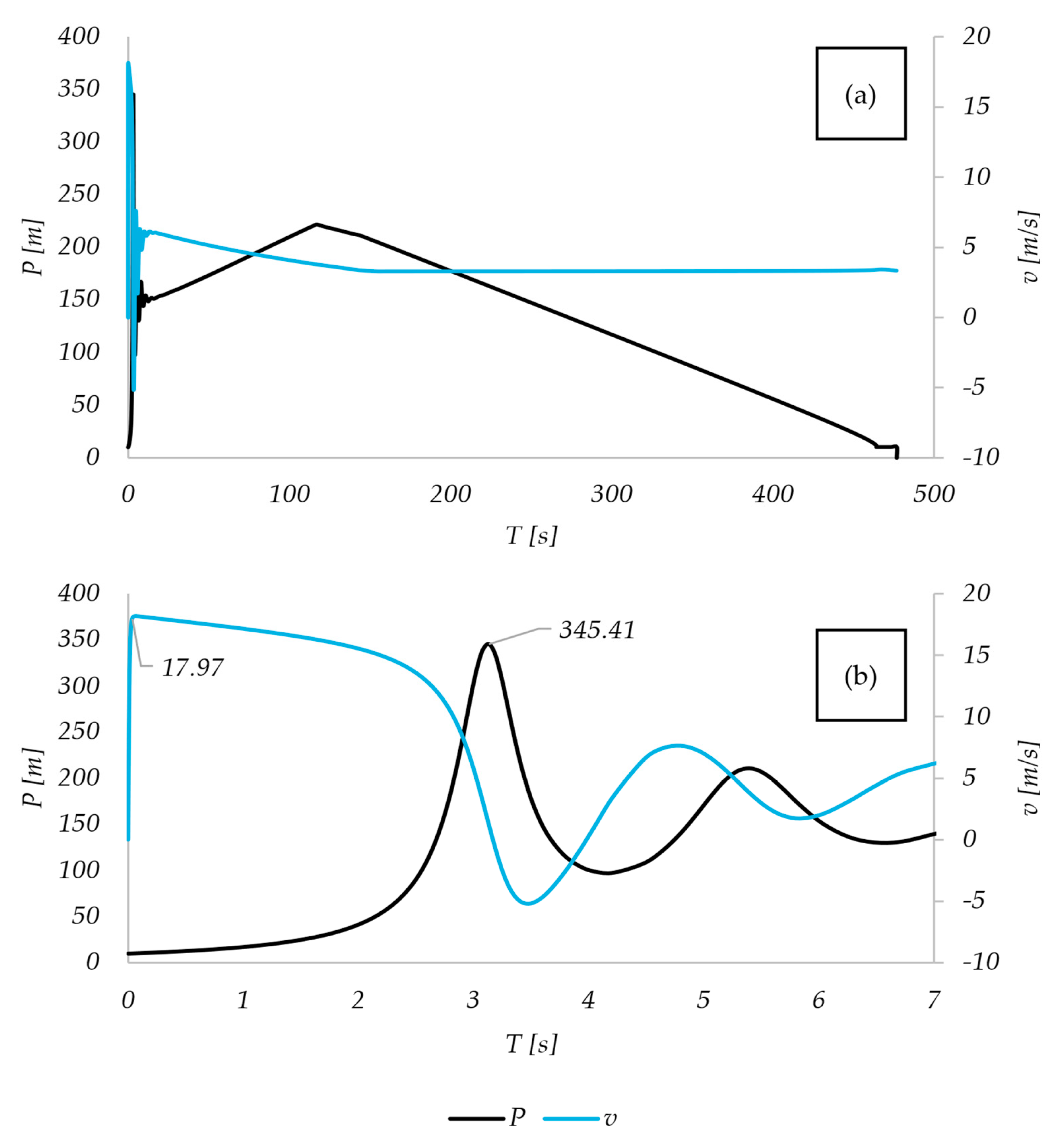
The following simulation results in this case for the following values: $D=0.30 \mathrm{m}$, ${\theta }_1=15°$, ${\theta }_2=15°$, $H_D=4 \mathrm{m}$, where $A_P=150$ and $C_P=80$, $k= 0.2$ and $L_{B1,0}=1100 \mathrm{m}$. Similarly, aspects such as valve opening, blockage column length and tank height were modified, where maximum pressures ranging from $42.62$ m to $345.41$ m were observed for block column lengths between $100 \mathrm{m}$ and $1150 \mathrm{m}$ and different openings, where it was evident that for the same opening but greater block column length, there was a higher pressure and velocity peak (Figure 7). For example, for a length of $L_{b,1}=700 \mathrm{m}$ with whole opening ($k = 0.2$), a pressure of 182.64 m was recorded, while for $L_{b,1}=1100 \mathrm{m}$ with the same coefficient, a value of 345.41 m was reached, which is consistent with the results obtained by Reference [23] where it was demonstrated that, based on rigid models, the size of the air pocket and the blocking column have the most significant impact on the peak pressure generated in the system. In turn, for a smaller air pocket (a larger blocking column), the air pocket compresses more abruptly at start-up, resulting in higher overpressure. Reference [51] experimentally demonstrated that for a similar system, peak pressures of up to seven times the inlet pressure to the system were generated, always in the first air pocket, which is identical to the studies previously conducted by Reference [52] with block lengths of 630 m and air pockets of 80 m reaching pressures of 277.00 m in 5.22 s.

After recording the maximum pressure peak $p_{max}^{*}$, a second overpressure peak generated by the damped oscillation of the system is evident, behaviour consistent with the rigid column model equations described above. This phenomenon occurs after the initial expansion of the air pocket, at which point the inertia of the filling column $H_D$ recompresses the air pocket before reaching static equilibrium. It is important to note that the magnitude of this second peak is lower than that of the first, an attenuation attributed to energy dissipation through friction along the pipe and to thermal dissipation inherent in the evolution of the trapped air.

3.2. Sensitivity Analysis Results

Based on the simulation results obtained using the Sensitivity Analyzer application, 2000 iterations were evaluated considering the value ranges for $D \in \left[0.160, 1.000\right] \mathrm{m}$, $H_D \in [1.002,4.998]\mathrm{ m}$, $k \in [0.208,23.994]$ $L_{B\mathrm{1,0}} \in [100.051,989.430]\mathrm{ m}$, ${\theta }_1 \in [-0.784,-0.101] rad$, and ${\theta }_2 \in \left[\mathrm{0.101,0.784}\right] rad$, which are reported in

Table 3. Input data range to sensitivity analysis.

Type	$\mathit{D}\left(\mathit{m}\right)$	${\mathit{H}}_{\mathit{D}}\left(\mathit{m}\right)$	$\mathit{k}$	${\mathit{L}}_{\mathit{B}\mathrm{1,0}}\left(\mathit{m}\right)$	${\mathit{\theta }}_1\left(\mathit{r}\mathit{a}\mathit{d}\right)$	${\mathit{\theta }}_2\left(\mathit{r}\mathit{a}\mathit{d}\right)$
Max	1.000	4.998	23.994	989.430	−0.101	0.784
Min	0.160	1.002	0.208	100.051	−0.784	0.100

.

The parameter bounds defined in Table 3 were selected based on hydraulic feasibility constraints, geometric limitations of the 1100 m pipeline system, and consistency with validated transient modelling studies involving entrapped air and filling operations [22,23,49]. These ranges ensure the physically realistic formation of entrapped air pockets and blocking columns whilst avoiding non-physical configurations, such as negative air volumes or geometrically infeasible column distributions. The selected bounds are therefore representative of pipeline filling and start-up conditions and are suitable for evaluating transient pressure amplification mechanisms. Furthermore, these parameter limits define the physically admissible domain within which the surrogate model is trained and applied, ensuring consistency between the simulated scenarios, the learned regression model, and the intended screening application.

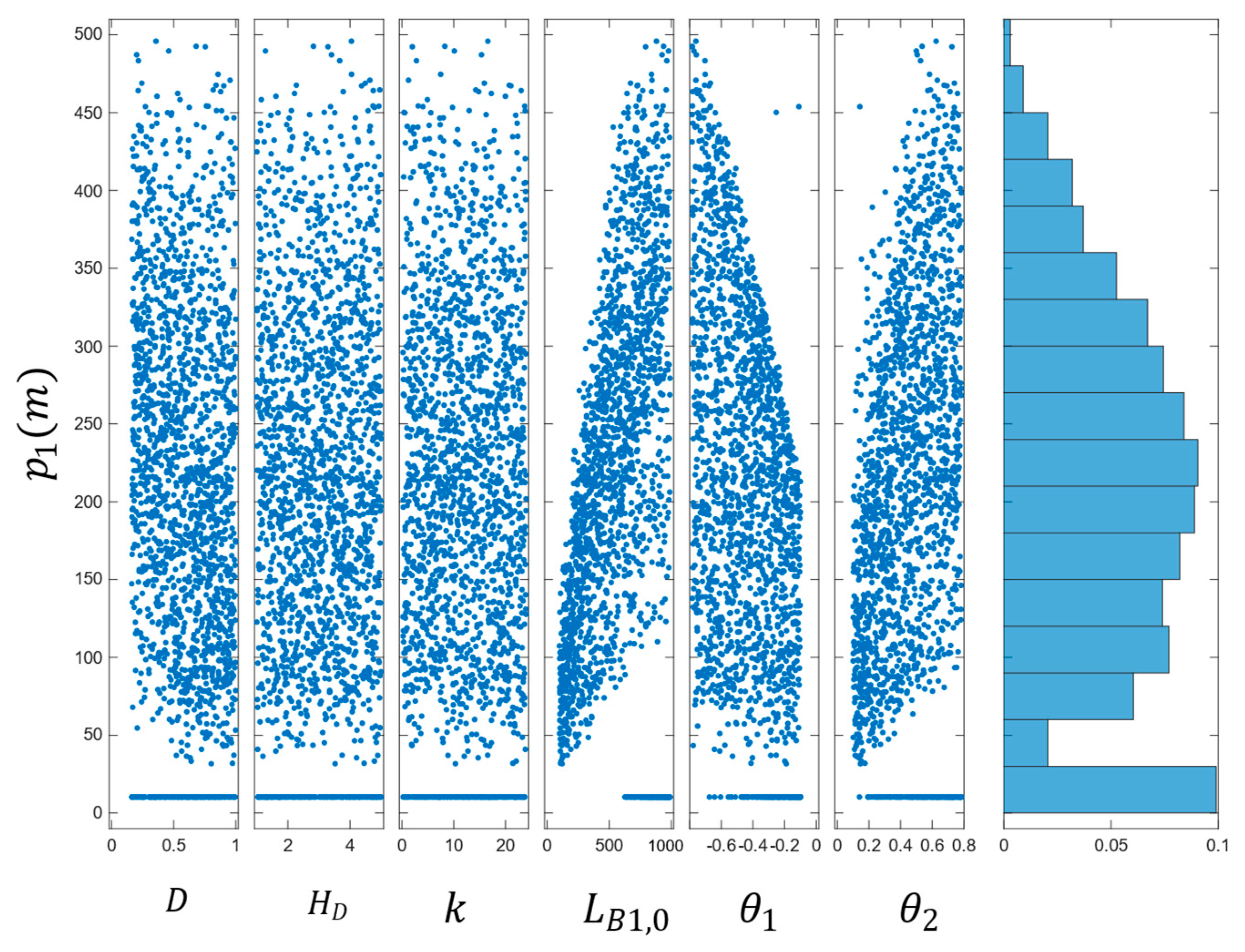
Figure 8 presents the modelling results of the simulated cases, where it can be observed that the model is identifiable according to the behaviour of parameters $L_{B\mathrm{1,0}}$, ${\theta }_1$, and ${\theta }_2$, with $p_1^{*}$ being directly proportional to these.

For the selected parameter ranges, 254 out of the 2000 simulated iterations (12.70%) exhibited a regime in which the filling and blocking columns merged within the pipeline, under the conditions specified in Equations (20) and (21). In these cases, the entrapped air pocket was displaced without undergoing significant compression, and the water column exited the conduit at near-atmospheric pressure, resulting in no transient pressure peak. This behaviour represents a physically valid operational regime characterised by negligible transient amplification rather than numerical instability. Because the objective of this study is to develop a surrogate model for predicting maximum pressure peaks associated with air-pocket compression, these scenarios were excluded from the regression dataset, as the target variable (maximum air-pocket pressure peak) is undefined or not representative of the transient amplification process. After filtering, a total of 1746 simulations with valid pressure peak formation were retained for surrogate model training and probabilistic risk analysis. This filtering ensures consistency between the physical phenomenon of interest and the surrogate modelling objective, whilst preserving the integrity of the statistical and physical interpretation of the transient behaviour. Since these excluded cases do not produce transient pressure peaks, their removal does not affect the surrogate model’s ability to learn peak-pressure behaviour or the interpretation of exceedance statistics within the physically relevant transient regime.

Additionally, the analysis of the scatter plots in Figure 8 highlights that the length of the blocking column ($L_{B\mathrm{1,0}}$) acts as the most influential factor in the generation of pressure peaks. A clear trend is observed in which the maximum recorded pressure increases significantly as the length of the blocking column increases, forming a well-defined upper envelope in the data distribution. This behaviour is physically attributed to the greater inertia associated with longer water columns, which, when coupled with the reduced volume of the entrapped air pockets typical of these configurations, results in more abrupt compressions and, consequently, higher overpressures during the start-up operation [53,54,55].

In contrast, the geometric parameters related to the pipeline alignment, specifically the slopes ${\theta }_1$, and ${\theta }_2$, show a direct correlation with $p_1^{\mathrm{*}}$, albeit with a higher degree of dispersion compared to the blocking length. This suggests that whilst gravitational acceleration affects the impact velocity, the system’s response is less predictable from the slope alone. On the other hand, the variables $D$, $H_D$, and $k$ display a uniform distribution without a discernible pattern in Figure 8, indicating that the maximum pressure is relatively insensitive to variations in diameter, tank head, or valve losses within the studied ranges, placing the geometric configuration of the air–water interface as the primary driver of the transient phenomena.

Data filtering was performed to ensure consistency between the modelling objective and the training dataset. Specifically, simulations in which the air pocket was expelled without generating a pressure peak were excluded, as the target variable (maximum air-pocket pressure) is undefined in such cases. This filtering step ensures that the surrogate model learns the relationship between input parameters and peak-pressure formation within the physically relevant transient regime.

Although uniform probability distributions were used for parameter sampling, the identified sensitivity patterns reflect the underlying deterministic hydraulic response rather than the assumed probability distribution. Whilst alternative distributions (triangular or truncated normal centred) would alter the frequency of occurrence of specific scenarios, they would not modify the physical response surface within the defined parameter bounds. Therefore, the identification of dominant predictors and exceedance behaviour is expected to remain robust with respect to the assumed sampling distribution for screening purposes.

3.3. Machine Learning Application

At this stage, 28 machine learning regression models were evaluated using RMSE, MAE, MSE, and R² on the validation and independent test sets (

Table 4. Test statistics results for the 28 ML models.

Model Type	RMSE Validation	MSE Validation	R2 Validation	MAE Validation	RMSE Test	MSE Test	R2 Test	MAE Test
Trilayered Neural Network	10.95	119.80	0.99	7.28	9.78	95.60	0.99	7.31
Matern 5/2 GPR	12.95	167.81	0.98	7.48	10.22	104.39	0.99	6.64
Rational Quadratic GPR	13.27	176.02	0.98	7.92	10.13	102.66	0.99	6.73
Squared Exponential GPR	13.51	182.64	0.98	8.41	9.85	97.03	0.99	6.67
Exponential GPR	13.61	185.13	0.98	8.72	14.25	203.03	0.98	8.63
Medium Gaussian SVM	14.90	221.96	0.98	10.56	15.39	236.77	0.98	10.62
Medium Neural Network	15.52	240.77	0.98	10.64	41.30	1705.58	0.87	30.45
Wide Neural Network	20.15	405.89	0.96	7.25	10.29	105.88	0.99	6.98
Bagged Trees	21.29	453.15	0.95	16.16	19.67	386.73	0.97	14.96
Least Squares Regression Kernel	22.99	528.34	0.95	16.95	26.23	688.14	0.95	19.21
Boosted Trees	26.17	685.10	0.93	19.74	26.55	704.66	0.95	18.61
Coarse Gaussian SVM	28.30	800.76	0.92	20.62	32.82	1077.28	0.92	22.25
Medium Tree	31.24	975.66	0.90	23.45	29.18	851.59	0.93	21.79
Cubic SVM	31.81	1012.10	0.90	24.62	36.95	1365.39	0.89	27.54
Fine Tree	31.89	1017.05	0.90	23.49	26.99	728.20	0.94	19.83
Stepwise Linear	32.90	1082.59	0.89	25.56	37.28	1390.01	0.89	28.63
Interactions Linear	33.13	1097.32	0.89	25.62	37.31	1392.11	0.89	28.50
Narrow Neural Network	36.14	1305.93	0.87	28.16	40.98	1679.39	0.87	30.33
Bilayered Neural Network	36.28	1315.88	0.87	28.14	10.40	108.23	0.99	7.12
Robust Linear	37.67	1418.85	0.86	29.93	45.21	2043.79	0.84	34.75
Linear	37.69	1420.45	0.86	30.28	45.47	2067.09	0.84	35.38
Coarse Tree	40.55	1644.57	0.84	31.62	36.92	1363.09	0.89	28.32
Quadratic SVM	43.70	1909.87	0.81	35.02	44.35	1967.36	0.85	33.82
Linear SVM	60.71	3685.89	0.63	49.85	61.20	3745.86	0.71	49.79
SVM Kernel	67.65	4576.39	0.54	54.86	60.71	3685.95	0.71	49.43
Fine Gaussian SVM	78.27	6126.15	0.39	61.43	82.51	6807.21	0.47	66.13
Efficient Linear SVM	94.21	8875.43	0.11	78.57	109.55	12000.52	0.07	95.17
Efficient Linear Least Squares	96.14	9242.32	0.08	80.22	111.68	12473.09	0.03	97.08

). The trilayered neural network achieved the best overall accuracy (RMSE = 10.95 m for validation; 9.78 m for test; MAE = 7.28 m for validation; 7.31 m for test; R² ≈ 0.99 in both). Several Gaussian Process Regression variants were similarly competitive (test RMSE ≈ 9.85–10.22 m; test MAE ≈ 6.64–6.73 m; R² ≈ 0.99). In contrast, efficient linear models performed poorly (validation RMSE ≈ 94–96 m; test RMSE ≈ 110–112 m; R² ≤ 0.11), confirming that linear forms cannot represent the nonlinear transient dynamics.

These patterns are consistent with the inductive biases of the models: kernel regularisation in Gaussian Process Regression and the nonlinear capacity of the neural network support accurate fits without large validation–test gaps, whereas strictly linear models underfit the transient dynamics within the sampled domain.

To ensure reproducibility, all Monte Carlo sampling and dataset partitioning were executed under a fixed random generator state (MATLAB rng(42,’twister’)). After filtering, 1746 peak-forming scenarios were retained. An independent test set of 174 samples (10.00%) was reserved exclusively for final evaluation. The remaining 1572 samples were split using holdout validation with 25% held out, resulting in 1179 training samples (67.50% of the full dataset) and 393 validation samples (22.50% of the full dataset). The split was purely random at the scenario level (no clustering/stratification was applied), and k-fold cross-validation or repeated-split experiments were not performed.

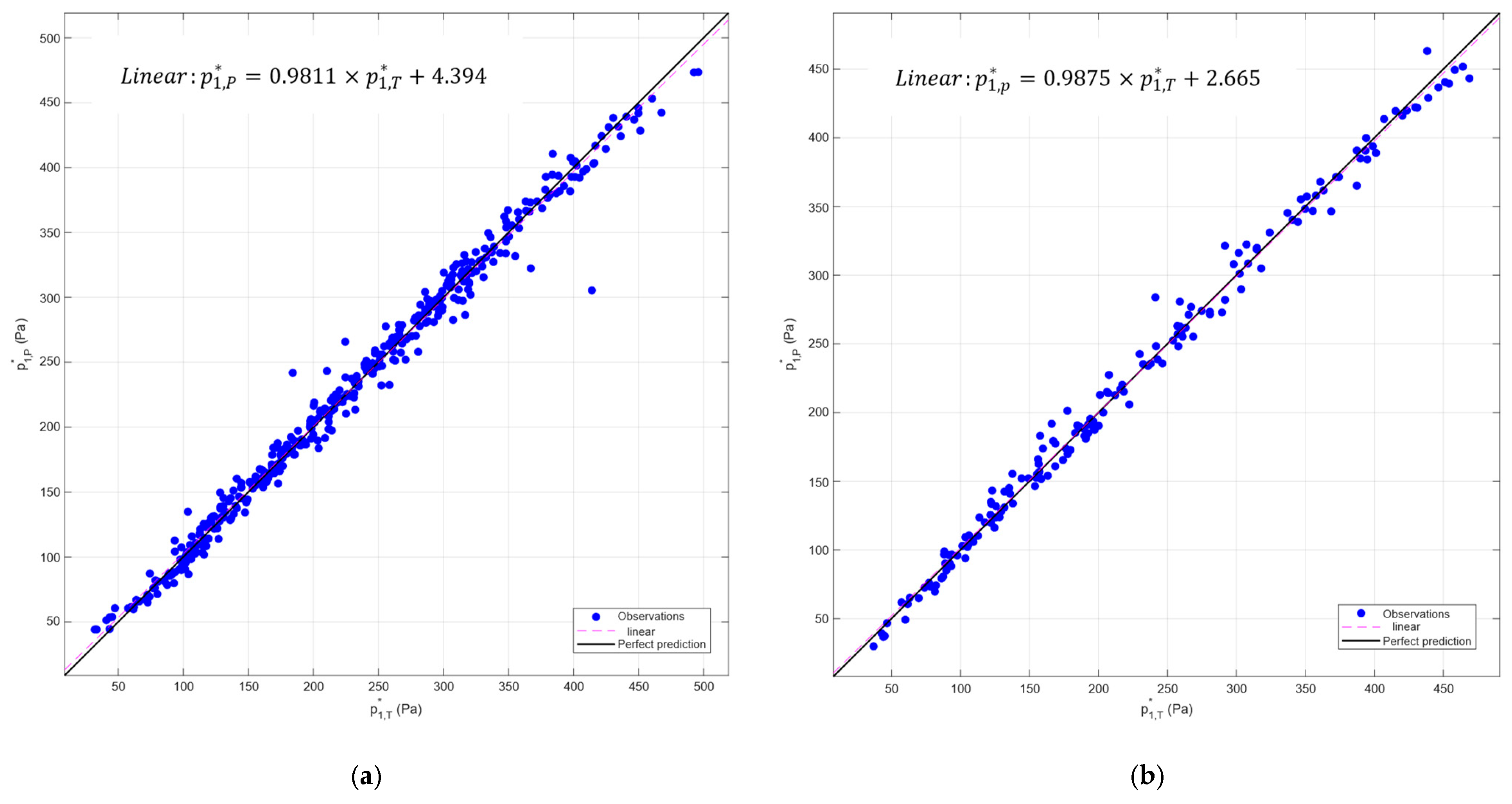
Figure 9 compares the simulated peak pressures with those predicted by the trilayered neural network for the validation and test subsets. In both cases, points cluster tightly around the 1:1 line across the full pressure range, including high-peak events. The fitted slopes (0.9811 for validation and 0.9875 for test) are close to unity and the intercepts (4.39 and 2.67 m) are small relative to the peak magnitudes, indicating low bias. Together with the close agreement between validation and test errors, these parity plots support the use of the network as an accurate surrogate within the sampled parameter domain.

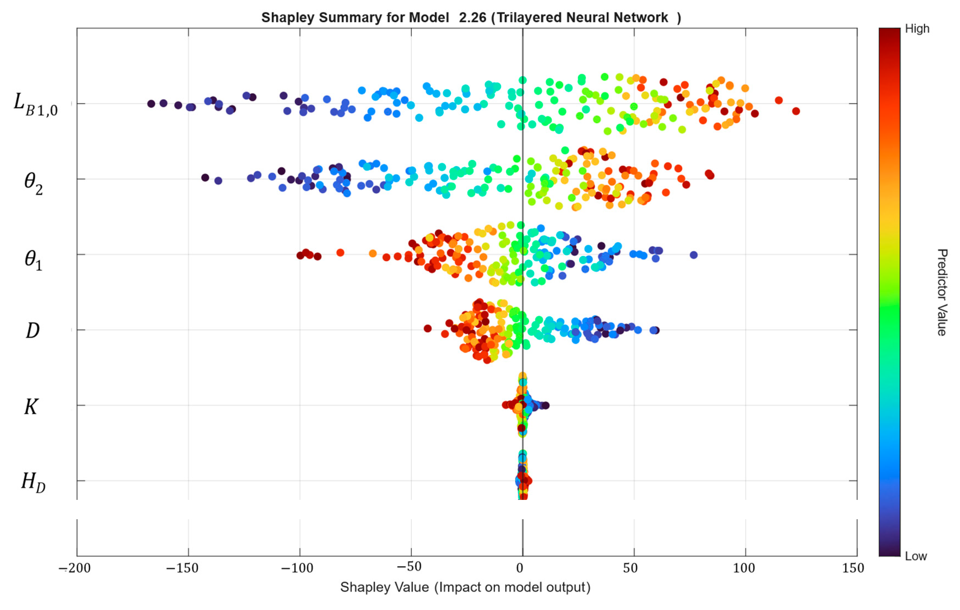
Figure 10 shows the Shapley analysis computed for the trilayered neural network model and indicates a robust hierarchy of predictor influence on maximum overpressure. $L_{B\mathrm{1,0}}$ dominates the explanation, exhibiting the widest spread of Shapley contributions, from approximately −170 to 120, which confirms it as the variable with the most significant capacity to shift the predicted peak response. High values of $L_{B\mathrm{1,0}}$ are predominantly associated with positive contributions, whereas low values tend to yield negative contributions. A second tier of importance is formed by ${\theta }_1$ and ${\theta }_2$, both exerting substantial effects but with opposing signs. ${\theta }_2$ follows an essentially direct pattern with Shapley values of roughly −120 to 80, increasing the estimated maximum overpressure. In contrast, ${\theta }_1$ displays an inverse behaviour with contributions of around −100 to 60, consistent with a mitigating effect. This contrast indicates that the model differentiates between geometric effects across pipe reaches, with one segment amplifying and the other attenuating the maximum response.

The predictor $D$ shows an intermediate influence, acting as a modulator, with Shapley values approximately in the range of −40 to 60. Smaller diameters are more frequently associated with positive contributions and larger diameters with negative contributions, albeit over a narrower impact range than $L_{B\mathrm{1,0}}$ and the slope-related predictors. Finally, $k$ and $H_D$ remain tightly clustered around zero, indicating a low overall contribution to maximum overpressure within the analysed data domain, with $k$ concentrated near −10 to 10 and $H_D$ near −5 to 5. Consequently, they do not govern the principal variability of the peak, and any influence is likely marginal or confined to conditions that are not prevalent in the training set.

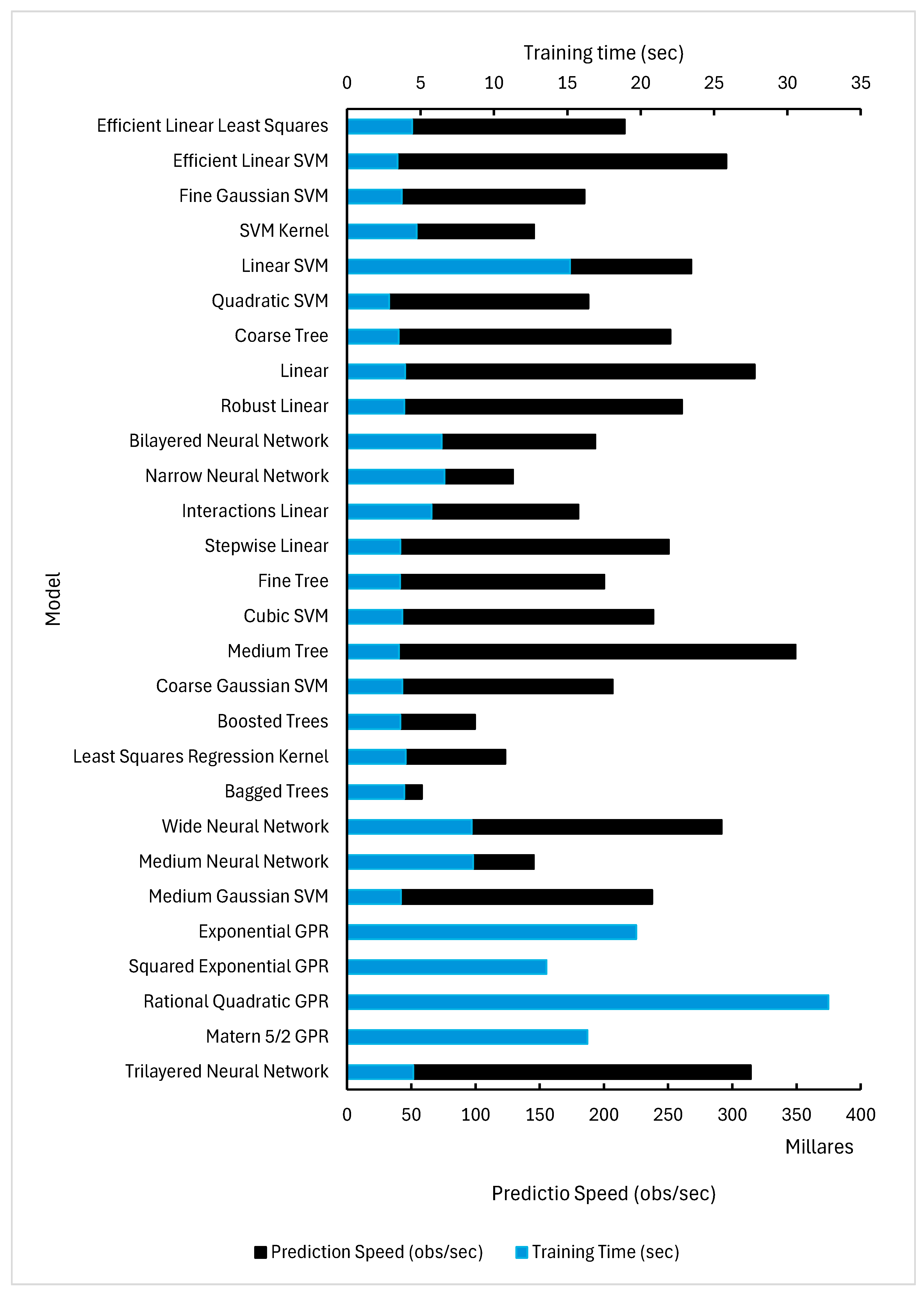
In addition to predictive accuracy, computational performance metrics reported in Figure 11 and

Table A2. ISO class for different materials for pipelines.

Material	ISO Class	Limit (m)
DI	PN25	254.93
DI	PN30	305.91
DI	PN40	407.89
DI	PN50	509.86
DI	PN64	652.62
HDPE	PN10	101.97
HDPE	PN12.5	127.46
HDPE	PN16	163.15
HDPE	PN20	203.94
HDPE	PN25	254.93
HDPE	PN6	61.18
HDPE	PN8	81.58
PVC-O	PN12.5	127.46
PVC-O	PN16	163.15
PVC-O	PN20	203.94
PVC-O	PN25	254.93
PVC-O	PN32	326.31
PVC-U	PN10	101.97
PVC-U	PN12.5	127.46
PVC-U	PN16	163.15
PVC-U	PN20	203.94
PVC-U	PN25	254.93
PVC-U	PN6	61.18
PVC-U	PN8	81.58

highlight important differences in efficiency among the evaluated regression models. Training times varied significantly depending on model complexity, ranging from approximately 3.4 s for efficient linear regression models to over 15 s for certain kernel-based and ensemble methods. The trilayered neural network achieved a favourable balance between training efficiency and predictive accuracy, with a training time of approximately 6.43 s. Prediction speed also exhibited substantial variation across model families, with simpler models such as decision trees and linear regression achieving speeds exceeding 300,000 observations per second, while more complex kernel-based methods required longer evaluation times. The trilayered neural network achieved a prediction speed of approximately 193,000 observations per second, enabling rapid evaluation of large numbers of transient scenarios. These results demonstrate that the selected surrogate model not only provides high predictive accuracy but also offers significant computational advantages compared to physics-based transient simulations, which require substantially longer execution times per scenario. This computational efficiency makes the surrogate model particularly suitable for Monte Carlo-based screening applications and real-time risk-informed operational assessment within the defined parameter domain.

4. Discussion

In references [22,51,53], the results confirm that entrapped air is the dominant mechanism governing transient overpressure during pipeline filling, as evidenced by the strong influence of the blocking column length and the high proportion of scenarios exceeding nominal pressure limits (Appendix A). Peak pressures of up to 345.41 m and exceedance rates reaching 97.53% for PN6 pipelines within the retained peak-forming subset (n = 1746) demonstrate the structural severity of uncontrolled filling operations conditional on uniform sampling. These findings are consistent with previous experimental and numerical studies, which have shown that rapid air-pocket compression and associated liquid-column inertia can generate transient pressures significantly exceeding nominal operating conditions.

Exceedance patterns across PN classes highlight the need for transient control strategies, consistent with prior analytical and numerical studies. The trilayered neural network accuracy (R² ≈ 0.99; RMSE = 9.78 m) shows that ML surrogates can reproduce nonlinear air–water transient dynamics efficiently, enabling rapid screening-based operational assessment [35,38]. From an engineering design perspective, these results define a screening-based design envelope that can guide early selection of start-up constraints and protection measures.

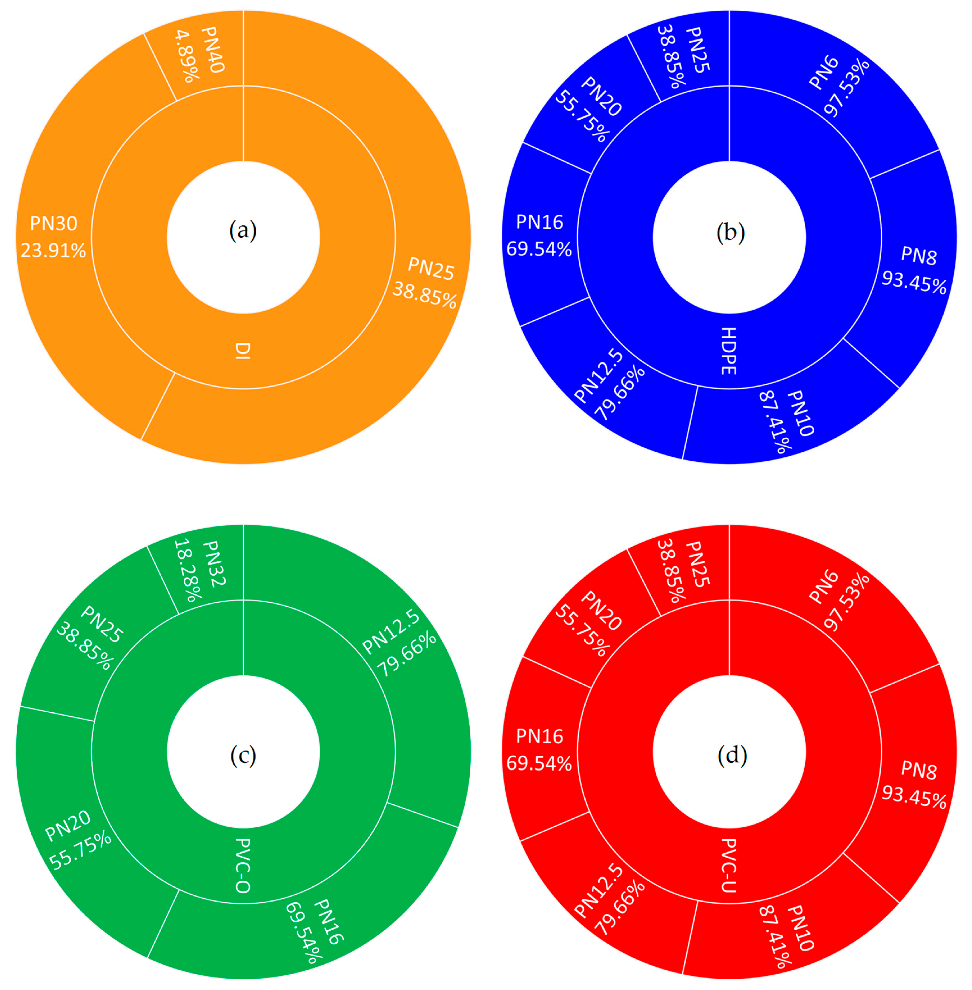
In this phase, peak pressures from the transient simulations were compared with ISO nominal pressure classes (PN) for common pipe materials (DI, HDPE, PVC-O, and PVC-U; Table A2). For each class, the continuous working-pressure limit was converted to head (m) and used as the threshold, and exceedance rates were computed over the retained peak-forming subset (n = 1746) (Figure 12). These exceedance rates are conditional screening metrics under uniform sampling within the admissible bounds and are not intended to represent field occurrence probabilities under utility-specific operating distributions. This comparison is framed as a design-check against international ISO PN class constraints within the screened scenario space.

The results demonstrate that criticality is concentrated in low PN classes. For PN6 (61.18 m), 1697 cases (97.53%) exceed the threshold; for PN8 (81.58 m), 1626 cases (93.45%); and for PN10 (101.97 m), 1521 cases (87.41%). Exceedance decreases with higher classes but remains substantial: PN12.5 (127.46 m) 1386 cases (79.66%); PN16 (163.15 m) 1210 cases (69.54%); PN20 (203.94 m) 970 cases (55.75%); and PN25 (254.93 m) 676 cases (38.85%). This trend indicates that, without transient control, many screened start-up manoeuvres can generate peaks above nominal class limits, supporting the need for operational mitigation in systems susceptible to entrapped air transients. Accordingly, the reported exceedance rates are interpreted as conditional screening prevalence within the defined design space, rather than field-frequency estimates.

Material selection reduces exceedance markedly at higher PN classes. For ductile iron, PN40 (407.89 m) is exceeded in 85 cases (4.89%), while PN50 (509.86 m) and PN64 (652.62 m) show no exceedances in the analysed scenarios. For PVC-O, PN32 (326.31 m) reduces exceedance to 318 cases (18.28%), although some critical events remain. Given the high exceedance prevalence in lower polymer classes, transient protection remains necessary (e.g., controlled start-up/shutdown ramps and suitable pressure-relief or damping devices) to keep peak pressures within the resistance capacity of pipes, joints, and fittings.

5. Conclusions

In this research, a simulation-driven screening framework was developed to evaluate peak pressures during pipeline start-up and filling with entrapped air, integrating rigid column transient modelling, Monte Carlo sampling, and machine learning surrogate modelling. From 2000 Monte Carlo-simulated start-up scenarios, 1746 peak-forming cases were retained after filtering and used to train and compare 28 regression model configurations. The trilayered neural network achieved the most consistent performance (R² = 0.99; RMSE = 10.95 m for validation; and 9.78 m for test), supporting its use as an efficient surrogate for rapid peak-pressure estimation within the evaluated parameter domain. The workflow was demonstrated on a representative filling case (two pipe sections, D = 0.30 m, longitudinal slopes, storage tank, pump characteristic curve, and control valve k = 0.20–24, without venting), enabling analysis of the gas-phase pressure response and operational applicability.

Interpretability analysis using dispersion plots and SHAP (Shapley Additive Explanations) consistently identified blocking-column length as the dominant driver of peak formation within the analysed ranges, exceeding the influence of slope and diameter. Relative to ISO nominal pressure classes (PN6–PN16), peak pressures exceeded nominal limits in 97.53% to 69.54% of the retained peak-forming scenarios (n = 1746) under uncontrolled manoeuvres. As these exceedance rates are conditional on uniform screening within the defined bounds, the proposed framework is best used to rapidly rank and screen operational configurations, supporting the selection of controlled filling strategies to reduce transient overpressure risk.

Design implications: (i) the framework enables rapid design-space screening of start-up strategies to identify feasible operating envelopes; (ii) it supports the selection of design and commissioning constraints (e.g., allowable peak head thresholds and ISO PN class checks) to reduce transient overpressure risk without extensive CFD-level computation.

References

1. Balacco, G.; Fontana, N.; Apollonio, C.; Giugni, M.; Marini, G.; Piccinni, A.F. Pressure Surges during Filling of Partially Empty Undulating Pipelines. ISH J. Hydraul. Eng. 2021, 27, 244–252. [Google Scholar] [CrossRef]
2. Laanearu, J.; Annus, I.; Koppel, T.; Bergant, A.; Vučković, S.; Hou, Q.; Tijsseling, A.S.; Anderson, A.; van’t Westende, J.M.C. Emptying of Large-Scale Pipeline by Pressurized Air. J. Hydraul. Eng. 2012, 138, 1090–1100. [Google Scholar] [CrossRef]
3. Romero, G.; Fuertes-Miquel, V.S.; Coronado-Hernández, Ó.E.; Ponz-Carcelén, R.; Biel-Sanchis, F. Transient Phenomena Generated in Emptying Operations in Large-Scale Hydraulic Pipelines. Water 2020, 12, 2313. [Google Scholar] [CrossRef]
4. Martinoia, T.; Barreto, C.V.; da Rocha, J.C.D.C.; Lavoura, J.; Henriques, F.M.P. Simulation and Planning of Pipeline Emptying Operations. In Proceedings of the Volume 1: Upstream Pipelines; Project Management; Design and Construction; Environment; Facilities Integrity Management; Operations and Maintenance; Pipeline Automation and Measurement; American Society of Mechanical Engineers: New York, NY, USA, 24 September 2012; pp. 603–611. [Google Scholar]
5. Fuertes-Miquel, V.S.; Coronado-Hernández, O.E.; Mora-Meliá, D.; Iglesias-Rey, P.L. Hydraulic Modeling during Filling and Emptying Processes in Pressurized Pipelines: A Literature Review. Urban Water J. 2019, 16, 299–311. [Google Scholar] [CrossRef]
6. Singh, M.K.; Kekatos, V. Optimal Scheduling of Water Distribution Systems. IEEE Trans. Control Netw. Syst. 2020, 7, 711–723. [Google Scholar] [CrossRef]
7. Ramos, H.; Covas, D.; Borga, A.; Loureiro, D. Surge Damping Analysis in Pipe Systems: Modelling and Experiments. J. Hydraul. Res. 2004, 42, 413–425. [Google Scholar] [CrossRef]
8. Chung, G.; Lansey, K. Application of the Shuffled Frog Leaping Algorithm for the Optimization of a General Large-Scale Water Supply System. Water Resour. Manag. 2009, 23, 797–823. [Google Scholar] [CrossRef]
9. Coronado-Hernández, O.E.; Fuertes-Miquel, V.S.; Besharat, M.; Ramos, H.M. Subatmospheric Pressure in a Water Draining Pipeline with an Air Pocket. Urban Water J. 2018, 15, 346–352. [Google Scholar] [CrossRef]
10. Ramezani, L.; Karney, B.W.; Profile, S.; Malekpour, A.; Asce, S.M.; Karney, B.; Asce, M.; Malekpour, A.; Asce, A.M. Encouraging Effective Air Management in Water Pipelines: A Critical Review. J. Water Resour. Plan. Manag. 2016, 142, 04016055. [Google Scholar] [CrossRef]
11. Zhou, L.; Liu, D.; Karney, B.; Zhang, Q. Influence of Entrapped Air Pockets on Hydraulic Transients in Water Pipelines. J. Hydraul. Eng. 2011, 137, 1686–1692. [Google Scholar] [CrossRef]
12. Wright, S.J.; Lewis, J.W.; Vasconcelos, J.G. Geysering in Rapidly Filling Storm-Water Tunnels. J. Hydraul. Eng. 2010, 137, 112–115. [Google Scholar] [CrossRef]
13. Maddahian, R.; Cervantes, M.J.; Bucur, D.M. Numerical Investigation of Entrapped Air Pockets on Pressure Surges and Flow Structure in a Pipe. J. Hydraul. Res. 2020, 58, 218–230. [Google Scholar] [CrossRef]
14. Zhou, L.; Liu, D.; Karney, B.; Wang, P. Phenomenon of White Mist in Pipelines Rapidly Filling with Water with Entrapped Air Pockets. J. Hydraul. Eng. 2013, 139, 1041–1051. [Google Scholar] [CrossRef]
15. Paternina-Verona, D.A.; Coronado-Hernández, O.E.; Espinoza-Román, H.G.; Fuertes-Miquel, V.S.; Ramos, H.M. Rapid Filling Analysis with an Entrapped Air Pocket in Water Pipelines Using a 3D CFD Model. Water 2023, 15, 834. [Google Scholar] [CrossRef]
16. Ramos, H.M.; Fuertes-Miquel, V.S.; Tasca, E.; Coronado-Hernández, O.E.; Besharat, M.; Zhou, L.; Karney, B. Concerning Dynamic Effects in Pipe Systems with Two-Phase Flows: Pressure Surges, Cavitation, and Ventilation. Water 2022, 14, 2376. [Google Scholar] [CrossRef]
17. Apollonio, C.; Balacco, G.; Fontana, N.; Giugni, M.; Marini, G.; Piccinni, A.F. Hydraulic Transients Caused by Air Expulsion during Rapid Filling of Undulating Pipelines. Water 2016, 8, 25. [Google Scholar] [CrossRef]
18. Aguirre-Mendoza, A.M.; Oyuela, S.; Espinoza-Román, H.G.; Coronado-Hernández, O.E.; Fuertes-Miquel, V.S.; Paternina-Verona, D.A. 2D CFD Modeling of Rapid Water Filling with Air Valves Using OpenFOAM. Water 2021, 13, 3104. [Google Scholar] [CrossRef]
19. Liou, C.P.; Hunt, W.A. Filling of Pipelines with Undulating Elevation Profiles. J. Hydraul. Eng. 1996, 122, 534–539. [Google Scholar] [CrossRef]
20. Martins, S.C.; Ramos, H.M.; Almeida, A.B. Conceptual Analogy for Modelling Entrapped Air Action in Hydraulic Systems. J. Hydraul. Res. 2015, 53, 678–686. [Google Scholar] [CrossRef]
21. Hurtado-Misal, A.D.; Hernández-Sanjuan, D.; Coronado-Hernández, O.E.; Espinoza-Román, H.; Fuertes-Miquel, V.S. Analysis of Sub-Atmospheric Pressures during Emptying of an Irregular Pipeline without an Air Valve Using a 2D CFD Model. Water 2021, 13, 2526. [Google Scholar] [CrossRef]
22. Fuertes-Miquel, V.S.; Coronado-Hernández, O.E.; Sánchez-Romero, F.J.; Saba, M.; Pérez-Sánchez, M. Assessing Air-Pocket Pressure Peaks During Water Filling Operations Using Dimensionless Equations. Mathematics 2025, 13, 267. [Google Scholar] [CrossRef]
23. Fuertes-Miquel, V.S.; López-Jiménez, P.A.; Martínez-Solano, F.J.; López-Patiño, G. Numerical Modelling of Pipelines with Air Pockets and Air Valves. Can. J. Civ. Eng. 2016, 43, 1052–1061. [Google Scholar] [CrossRef]
24. Tijsseling, A.S.; Hou, Q.; Bozkuş, Z.; Laanearu, J. Improved One-Dimensional Models for Rapid Emptying and Filling of Pipelines. J. Press. Vessel Technol. 2016, 138, 031301. [Google Scholar] [CrossRef]
25. Bentley HAMMER CONNECT Edition Rigid Column Theory. Available online: https://docs.bentley.com/LiveContent/web/Bentley%20HAMMER%20SS6-v1/en/GUID-F87F1515-85CE-4FF3-9C5F-3AD5E427F125.html (accessed on 25 February 2025).
26. Zeng, W.; Zecchin, A.C.; Lambert, M.F. Elastic Water Column Model for Hydraulic Transient Analysis of Pipe Networks. J. Hydraul. Eng. 2022, 148, 04022027. [Google Scholar] [CrossRef]
27. Wiggert, D.C.; Tijsseling, A.S. Fluid Transients and Fluid-Structure Interaction in Flexible Liquid-Filled Piping. Appl. Mech. Rev. 2001, 54, 455–481. [Google Scholar] [CrossRef]
28. Bergant, A.; Simpson, A.R.; Tijsseling, A.S. Water Hammer with Column Separation: A Historical Review. J. Fluids Struct. 2006, 22, 135–171. [Google Scholar] [CrossRef]
29. Nerella, R.; Venkata Rathnam, E. Fluid Transients and Wave Propagation in Pressurized Conduits Due to Valve Closure. Procedia Eng. 2015, 127, 1158–1164. [Google Scholar] [CrossRef]
30. Cheng, D.; Cao, Z. A General Double Layer-Averaged Model for Water–Air Two-Phase Pipe Flows. Int. J. Multiph. Flow 2025, 185, 105136. [Google Scholar] [CrossRef]
31. Meziou, A.; Khan, Z.; Wassar, T.; Franchek, M.A.; Tafreshi, R.; Grigoriadis, K. Dynamic Modeling of Two-Phase Gas/Liquid Flow in Pipelines. SPE J. 2019, 24, 2239–2263. [Google Scholar] [CrossRef]
32. He, J.; Hou, Q.; Lian, J.; Tijsseling, A.S.; Bozkus, Z.; Laanearu, J.; Lin, L. Three-Dimensional CFD Analysis of Liquid Slug Acceleration and Impact in a Voided Pipeline with End Orifice. Eng. Appl. Comput. Fluid Mech. 2022, 16, 1444–1463. [Google Scholar] [CrossRef]
33. Payares Guevara, C.R.; Patiño-Vanegas, A.; Pereira-Batista, E.; Coronado-Hernández, O.E.; Fuertes-Miquel, V.S. An Analytical Model for the Prediction of Emptying Processes in Single Water Pipelines. Appl. Sci. 2025, 15, 6000. [Google Scholar] [CrossRef]
34. García-Todolí, S.; Iglesias-Rey, P.L.; Mora-Meliá, D.; Martínez-Solano, F.J.; Fuertes-Miquel, V.S. Computational Determination of Air Valves Capacity Using CFD Techniques. Water 2018, 10, 1433. [Google Scholar] [CrossRef]
35. Burgos-Méndez, Ó.J.; Coronado-Hernández, O.E.; Ramos, H.M.; Arrieta-Pastrana, A.; Pérez-Sánchez, M. Water Hammer Mitigation Using Hydro-Pneumatic Tanks: A Multi-Criteria Evaluation of Simulation Tools and Machine Learning Modelling. Water 2025, 17, 1883. [Google Scholar] [CrossRef]
36. Martínez-Padilla, E.A.; Arrieta-Pastrana, A.; Coronado-Hernández, O.E.; Saba, M.; Fuertes-Miquel, V.S. Predictive Analysis for U-Tube Transient Flow Events: A Digitalisation Framework. Fluids 2025, 10, 247. [Google Scholar] [CrossRef]
37. Demuth, H.; Beale, M. Neural Network Toolbox for Use with MATLAB User’s Guide; MathWorks, Inc.: Natick, MA, USA, 1992. [Google Scholar]
38. Li, H.; Zhang, Y.; Cui, J.; Zhang, F.; Yang, X.; Shi, W.; Mao, L. Optimization of Water Hammer Protection against Sudden Pump Stoppage Using Machine Learning Models and Intelligent Algorithms. J. Hydraul. Res. 2025, 63, 265–277. [Google Scholar] [CrossRef]
39. Ayati, A.H.; Haghighi, A.; Ghafouri, H.R. Two-Stage Model for Machine Learning/Transient-based Leak Detection in Pressurized Pipelines. Res. Sq. 2022. ahead of printing. [Google Scholar] [CrossRef]
40. Sharma, S.; Agyeman, B.T.; Palimi, M.; Liu, J.; Zhang, X. Machine Learning-Driven Pressure Drop Prediction in Multiphase Slurry Hydrotransport. Powder Technol. 2025, 465, 121314. [Google Scholar] [CrossRef]
41. Goda, T. A Simple Algorithm for Global Sensitivity Analysis with Shapley Effects. Reliab. Eng. Syst. Saf. 2021, 213, 107702. [Google Scholar] [CrossRef]
42. Mosavi, A.; Ozturk, P.; Chau, K. Flood Prediction Using Machine Learning Models: Literature Review. Water 2018, 10, 1536. [Google Scholar] [CrossRef]
43. The MathWorks, Inc. Statistics and Machine Learning ToolboxTM User’s Guide R2025b; MathWorks, Inc.: Natick, MA, USA, 1993. [Google Scholar]
44. Afoufou, F.; Abda, Z.; Toumi, A.; Sekiou, F. Modeling and Simulation of Water Hammer Phenomena Using Artificial Neural Networks (ANN). Water 2025, 17, 1617. [Google Scholar] [CrossRef]
45. Wang, X. Uncertainty Quantification and Global Sensitivity Analysis for Transient Wave Propagation in Pressurized Pipes. Water Resour. Res. 2021, 57, e2020WR028975. [Google Scholar] [CrossRef]
46. Yan, H.; Li, S.; Tian, W.; Wang, J.; Li, F.; Duan, H.; Tao, T.; Xin, K. A Hybrid Model Coupling Data and Hydraulic Transient Laws for Water Distribution Systems. Water Resour. Res. 2025, 61, e2023WR036641. [Google Scholar] [CrossRef]
47. Jones, M.N.; Frutiger, J.; Ince, N.G.; Sin, G. The Monte Carlo Driven and Machine Learning Enhanced Process Simulator. Comput. Chem. Eng. 2019, 125, 324–338. [Google Scholar] [CrossRef]
48. Farinango, P.; Estrada, R.; Vera, N. Evaluation of Indoor Positioning System Design Based on Empirical Propagation Models versus Optimizable Regression Models. Procedia Comput. Sci. 2025, 265, 301–309. [Google Scholar] [CrossRef]
49. Paternina-Verona, D.A.; Coronado-Hernández, O.E.; Espinoza-Román, H.G.; Arrieta-Pastrana, A.; Tasca, E.; Fuertes-Miquel, V.S.; Ramos, H.M. Attenuation of Pipeline Filling Over-Pressures through Trapped Air. Urban Water J. 2024, 21, 698–710. [Google Scholar] [CrossRef]
50. Coronado-Hernández, O.E. Trasient Phenomena During the Emptying Process of Water in Pressurized Pipelines. Ph.D. Thesis, Universitat Politècnica de València, València, Spain, 2019. [Google Scholar]
51. Zhou, L.; Liu, D.; Karney, B. Investigation of Hydraulic Transients of Two Entrapped Air Pockets in a Water Pipeline. J. Hydraul. Eng. 2013, 139, 949–959. [Google Scholar] [CrossRef]
52. Izquierdo, J.; Fuertes, V.S.; Cabrera, E.; Iglesias, P.L.; Garcia-Serra, J. Pipeline Start-up with Entrapped Air. J. Hydraul. Res. 1999, 37, 579–590. [Google Scholar] [CrossRef]
53. Bergant, A.; Tijsseling, A.; Kim, Y.i.; Karadžić, U.; Zhou, L.; Lambert, M.F.; Simpson, A.R. Unsteady Pressures Influenced by Trapped Air Pockets in Water-Filled Pipelines. J. Mech. Eng. 2018, 64, 501–512. [Google Scholar] [CrossRef]
54. Romero, G.; Fuertes-Miquel, V.S.; Coronado-Hernández, Ó.E.; Ponz-Carcelén, R.; Biel-Sanchis, F. Analysis of Hydraulic Transients during Pipeline Filling Processes with Air Valves in Large-Scale Installations. Urban Water J. 2020, 17, 568–575. [Google Scholar] [CrossRef]
55. Abreu, J.; Cabrera, E.; Espert, V.B. Transitorios Hidráulicos: Del Régimen Estacionario al Golpe Ariete; Editorial de la Universidad Politécnica de Valencia: Valencia, Spain, 2012; ISBN 9788490486603. [Google Scholar]
56. ISO 2531:2009; Ductile Iron Pipes, Fittings, Accessories and Their Joints for Water Applications. International Organization for Standardization: Geneva, Switzerland, 2009.
57. ISO 4427-2:2019; Plastics Piping Systems for Water Supply, and for Drainage and Sewerage Under Pressure—Polyethylene (PE) Part 2: Pipes. International Organization for Standardization: Geneva, Switzerland, 2019.
58. ISO 152-2:2009; Plastics Piping Systems for Water Supply and for Buried and Above-Ground Drainage and Sewerage Under Pressure—Unplasticized Poly(Vinyl Chloride) (PVC-U) Part 2: Pipes. International Organization for Standardization: Geneva, Switzerland, 2009.
59. ISO 16422-1:2024; Pipes and Joints Made of Oriented Unplasticized Poly(Vinyl Chloride) (PVC-O) for the Conveyance of Water Under Pressure Part 1: General. International Organization for Standardization: Geneva, Switzerland, 2024.
Figure 1. Methodology employed in this study.
Designs 10 00039 g001
Figure 2. General scheme of the system.
Designs 10 00039 g002
Figure 3. Methodology for generating multiple automatic simulations.
Designs 10 00039 g003
Figure 4. A trilayered neural network architecture is used for surrogate modelling of transient pressure peaks. Arrows indicate the direction of forward information flow from input predictors through successive hidden layers to the output node representing the maximum absolute air-pocket pressure peak.
Designs 10 00039 g004
Figure 5. Common transfer function graphs.
Designs 10 00039 g005
Figure 6. Scheme of filling process in two pipes without an air valve.
Designs 10 00039 g006
Figure 7. Evolution of the transient event: air pocket pressure and water velocity for full (a) and peak range (b).
Designs 10 00039 g007
Figure 8. Results of sensitivity analysis.
Designs 10 00039 g008
Figure 9. Comparison between predicted and true air-pocket pressure: (a) validation stage; and (b) testing stage.
Designs 10 00039 g009
Figure 10. Shapley for the trilayered neural network.
Designs 10 00039 g010
Figure 11. Prediction speed and training time for all regression models.
Designs 10 00039 g011
Figure 12. Proportion of pressures exceeding the maximum capacities of different commercial pipes. Note: (a) DI: Ductile Iron, (b) HDPE: High-Density Polyethylene, PN: Nominal Pressure for HDPE pipes, (c) PVC-O = Oriented Polyvinyl Chloride; and (d) PVC-U: Unplasticized Polyvinyl Chloride. Percentages are computed over the retained peak-forming subset (n = 1746) [56,57,58,59].
Designs 10 00039 g012