1. Introduction
In recent years, the demand for personalized design has grown rapidly, driven by increasingly diverse user preferences, lifestyle patterns, and functional requirements, especially in the fields of architecture and urban planning [
1,
2]. Residential layout design is no longer expected to only satisfy basic spatial constraints but also to support personalized living habits, functional rationality, and adaptive use of space [
3,
4]. This practical demand has highlighted the limitations of traditional one-size-fits-all design paradigms and motivated the exploration of intelligent, data-driven layout generation methods capable of balancing personalization, efficiency, and design quality [
5].
Recent advances in machine learning, particularly generative models, have shown great promise in addressing these challenges [
6]. Among these, Variational Autoencoders (VAEs) have gained considerable attention for their ability to model complex data distributions and generate diverse outputs [
7]. However, traditional VAEs suffer from limitations in terms of controllability, particularly when generating layouts tailored to specific user needs. To improve control over generated outputs, Conditional Variational Autoencoders [
3] (CVAEs) have been introduced, which condition the model on specific variables, such as user preferences or functional requirements [
8]. Despite their success in various domains, CVAEs still face challenges such as latent space redundancy and difficulty in capturing complex relationships between layout components, which are essential for generating functional and diverse designs.
Researchers have made significant progress in addressing challenges in layout generation. For example, Ye et al. [
9] developed a method for generating structurally coherent house layouts with global consistency by encoding rooms and their spatial relationships in a graph structure, capturing inter-room interactions to improve layout optimization. Similarly, Tang et al. [
10] proposed Graph Transformer GANs (GTGANs), which leverage graph convolutions and self-attention within a Transformer-based generator. By employing connected and non-connected node attention, GTGAN better captures both global and local relationships, resulting in optimized architectural layouts. Azmeraw et al. [
11] reviewed and categorized computational methods for house floor plan generation, highlighting both procedural and deep generative approaches.
Further advancements include LGGAN, introduced by Kangjie Li et al. [
12], a generative adversarial network for mechanical layout generation featuring hierarchical generation, noise reduction, and size refinement, with an active learning strategy for efficient convergence with limited data. Cheng et al. [
13] developed a method for land-use layout design in virtual worlds, ensuring high-quality output through geometric and planning objectives. Chen et al. [
14] proposed EcGAN, an element-conditioned GAN that enhances bounding box modeling for graphic layouts using an element mask, element condition loss, and two-step discriminators. Zhao et al. [
15] introduced Layout2Im, a method that generates images from layouts by disentangling object representations into specified categories and uncertain appearances, combining word embeddings and low-dimensional vectors with convolutional LSTM. In addition, Ayçam et al. [
16] investigated traditional Diyarbakir house forms and settlement patterns, demonstrating that their adaptation can improve energy efficiency and sustainability in modern housing. Finally, Zakraoui et al. [
17] proposed a three-stage story-to-image generation method with object layout guidance, showing improved semantic accuracy and realism compared to existing approaches.
Although existing methods have advanced layout generation, they often optimize only one or two aspects, such as structural coherence or visual quality, neglecting holistic balance. Current models rarely address four core challenges simultaneously: (1) controllability, guided by user preferences and constraints; (2) diversity, avoiding mode collapse and supporting varied outcomes; (3) functional rationality, ensuring layouts follow realistic spatial logic; and (4) training efficiency, critical for practical deployment but often limited by complex models or slow convergence. This gap motivates a unified framework. Practical integration of generative tools into architecture and AI domains remains limited. Methods that incorporate architectural constraints, functional requirements, and user preferences provide preliminary real-world validation.
To address these gaps, this paper proposes HCVEA, a hybrid controllable variational framework for residential layout generation. It integrates an improved CVAE, a CTC-Attention decoder, and the A3C reinforcement learning algorithm. The CVAE enhances latent space expressiveness for controllability and diversity, the CTC-Attention captures complex contextual dependencies for functional rationality, and A3C improves training efficiency through parallelized optimization. By coordinating these components within a unified architecture, HCVEA simultaneously addresses the four core challenges while aligning with practical architectural requirements, validated through controlled experiments. Contributions of this paper include the following:
- (i)
Enhanced latent space structure: HCVEA introduces a flexible, structured latent space with gradient stability and conditioned prior, distinguishing it from traditional CVAEs. It reduces redundancy, prevents homogenization, and enables controllable and diverse layouts, addressing CVAE limitations in personalized layout generation.
- (ii)
Reinforcement learning integration: A3C encodes architectural rules in the reward, unlike prior CVAE/GAN/graph-based models. It ensures rule compliance, improves functional rationality, and aligns layouts with user preferences, targeting the limitations of rule-based and graph-based methods.
- (iii)
CTC-Attention decoder: We extend CTC from temporal to spatial sequences, converting 2D layout relationships into topology-aware 1D sequences and combining CTC soft alignment with attention. This addresses graph-based model limitations, enhancing functional zoning and room adjacency coherence.
- (iv)
A3C reinforcement learning algorithm: A parallel A3C framework is tightly coupled with CTC-Attention decoding. The reward function aligns with spatial sequence features, and the action space supports fine-grained layout adjustments, enabling closed-loop optimization that accelerates convergence and ensures architectural rule compliance.
- (v)
Practical integration and proof-of-concept validation: HCVEA aligns with real-world architectural needs by incorporating spatial rules, user preferences, and functional constraints. Preliminary experiments confirm its effectiveness and feasibility for practical residential layout design, overcoming the limitations of existing tools.
4. Methodology
4.1. Model Framework Overview
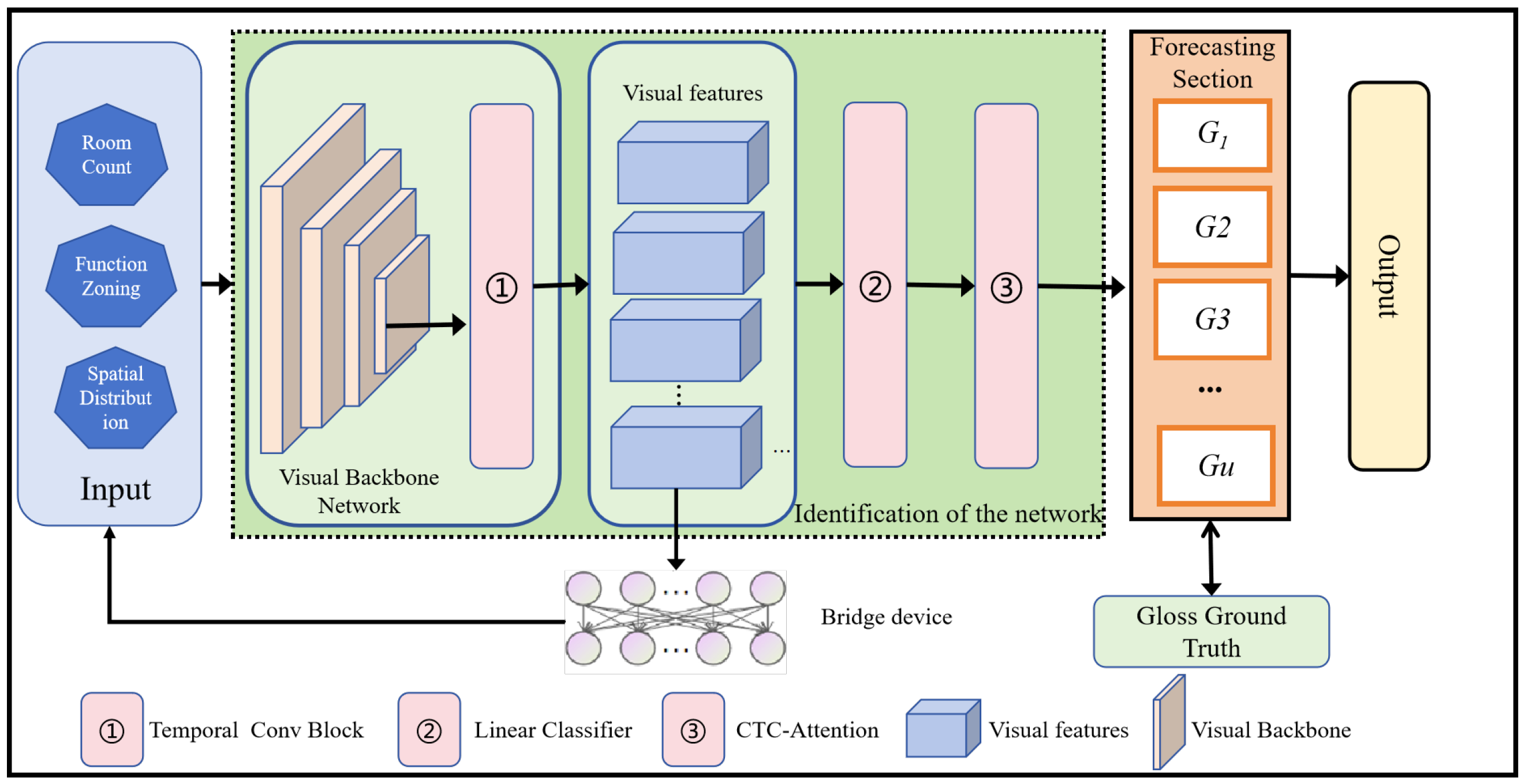
The HCVEA model integrates advanced techniques such as CVAE, RL, and a novel decoding mechanism to generate personalized and flexible residential layouts. By combining generative modeling with optimization, the model overcomes the limitations of traditional methods, enabling highly adaptable designs that meet both functional and aesthetic requirements. The framework operates through several key stages, each contributing to the creation of diverse and contextually coherent floor plans, as illustrated in
Figure 1.
Input Conditioning and Latent Space Encoding: The model conditions on user preferences and design constraints, such as room types, spatial distributions, and functional zoning, which guide the encoder to map data into a structured latent space. The encoder uses three Conv2d layers (3→64→128→256 channels, kernel = 3, stride = 2, padding = 1) followed by two fully connected layers projecting the 256 dim convolutional features to a 128 dim latent space for mean and variance, ensuring structured and diverse latent representations.
Layout Generation and Refinement: With the latent space established, the decoder generates an initial layout based on the encoded information. The decoder employs three symmetric ConvTranspose2d layers with batch normalization and ReLU to reconstruct layouts while preserving feature hierarchies. An RL agent then iteratively refines room placements using a reward function that enforces user preferences and spatial constraints, ensuring functional and aesthetically coherent designs.
VAE Loss Optimization: The VAE loss function is modified to include a gradient-based stability term for improved training stability and latent space regularization. Specifically, the loss is defined as , where the gradient term is computed over the latent space with batch size 32 and latent dimension 128. This ensures both accurate reconstruction and controlled latent representation.
Contextual Refinement with CTC-Attention: To enhance spatial coherence and room relationships, the model uses a CTC-Attention decoder. This mechanism focuses on key layout features like room adjacency and spatial dependencies, improving functional zoning and overall layout quality.
Multi-Level Refinement and Output: The layout is refined through a multi-level process, starting with high-level zoning and spatial arrangement, followed by adjustments to room sizes and configurations. The final layout is produced, meeting user requirements and maintaining spatial coherence.
The overall algorithm flow is summarized in Algorithm 1, which outlines the steps involved in the layout generation and refinement process.
| Algorithm 1 Overall algorithm flow |
- 1:
Input: User preferences c, initial layout x - 2:
Output: Optimized layout - 3:
Encode input layout and conditions into latent space: - 4:
Generate initial layout: - 5:
Minimize VAE loss: - 6:
Refine layout using CTC-Attention decoder - 7:
Refine layout with RL: compute reward and update layout - 8:
Perform multi-level spatial refinement: - 9:
Return: Optimized layout
|
4.2. HCVEA Architecture
Existing CVAE, GAN, and graph-based models often yield homogeneous layouts, miss continuous spatial dependencies, and face large-scale training inefficiency. HCVEA overcomes these issues by integrating an enhanced CVAE, a CTC-Attention decoder, and A3C reinforcement learning, enabling controllable, diverse, and functionally rational layouts. Encoder/decoder structures, latent mappings, and gradient-based VAE loss are explicitly defined to ensure reproducibility.
Given an input layout
x and auxiliary conditions
c, the model learns a latent variable
z that captures these conditions. The goal is to optimize the ELBO with the following loss function:
The loss function consists of three components: the reconstruction term , ensuring layout x is reconstructed from the latent variable z conditioned on x and c; the regularization term , minimizing the divergence between posterior and prior distributions, controlled by ; and the gradient-based stability term , which prevents overfitting and improves stability. Together, these components optimize the model’s ability to generate high-quality layouts while maintaining latent space flexibility.
The decoder uses a CTC-based attention mechanism to refine the layout based on
z. The attention weights
, which guide the focus on relevant areas of the layout, are calculated as
Here,
measures the relevance between rooms
i and
j based on their latent representations
and
. The attention weight for room
i is computed by evaluating the relevance to all rooms
j, and normalizing it across all pairs. This ensures the attention weights sum to 1, helping the decoder focus on spatially related rooms and improving layout coherence. The final layout
is generated by the decoder, which takes the latent variable
z and the attention weights
as inputs:
Here, the decoder aggregates the contributions of all rooms
i by weighting each room’s latent representation
with the attention weight
, ensuring a spatially coherent layout where the decoder focuses more on relevant room configurations. The RL objective is defined as
In this equation,
represents the reward at time step
t, depending on the current layout configuration
and the agent’s parameters
, with
being the discount factor that prioritizes earlier rewards. The RL agent uses this objective to iteratively refine the layout, improving it based on user preferences and constraints. Finally, the total loss function that combines the VAE, RL refinement, and latent space regularization is expressed as
This loss function integrates the VAE loss , the reinforcement learning (RL) loss , and a latent space regularization term, with and as balancing hyperparameters controlling the contributions of RL and regularization.
4.3. Latent Space Enhancement
Traditional CVAEs often produce redundant latent spaces, leading to homogenized layouts and limited controllability. We refine the latent variable
z by incorporating a conditioned prior and a gradient stabilization term, ensuring diverse, controllable, and informative latent representations for layout generation.The encoder outputs a Gaussian distribution
over the latent variable
z, conditioned on the input layout
x and auxiliary conditions
c:
Here,
and
represent the mean and variance of the latent distribution, capturing the structure of
x and conditioning variables
c. To regularize the latent space, we minimize the Kullback–Leibler divergence between the posterior
and the prior
:
It is crucial to distinguish HCVEA’s gradient stabilization term from existing VAE regularization methods, as they differ in design philosophy and optimization targets.
- (1)
Difference in -VAE: -VAE scales the KL term with a hyperparameter to encourage latent disentanglement, focusing on statistical alignment of latent dimensions. Excessive disentanglement may fragment spatial structures in layout generation. In contrast, HCVEA’s gradient stabilization term directly controls the gradient sensitivity of the reconstruction function with respect to latent variables, penalizing large changes to maintain functional stability, spatial coherence, and room adjacency, while reducing latent redundancy.
- (2)
Difference from implicit regularization methods: Techniques such as weight decay, dropout, or data augmentation impose indirect constraints on parameters or inputs but do not explicitly regulate the latent space or reconstruction. HCVEA’s gradient stabilization term explicitly enforces smooth, predictable mappings from latent variables to layout features. The tunable hyperparameter (set to 0.2) balances robustness and reconstruction fidelity, enabling diverse, accurate, and functionally rational layouts.
Together, the KL term, conditioned prior, and gradient stabilization term form the latent space objective, ensuring that HCVEA learns a stable, flexible latent space suitable for generating diverse, spatially coherent, and functionally rational layouts.
4.4. CTC-Attention Decoder
Existing models, including GANs and graph-based frameworks, often fail to capture continuous spatial dependencies between rooms, leading to disordered functional zoning [
28]. To address this, we convert the 2D floor plan into a structured 1D sequence preserving spatial relationships such as room adjacency and functional zoning. The 256 × 256 layout is divided into 8 × 8 patches, each encoding functional type (8D one-hot), boundary (1D), and relative position (2D). Patches in the same functional zone are grouped consecutively, producing a sequence
of length 800–1200.
The CTC-Attention decoder aligns V with the target configuration while focusing on spatially relevant features. CTC handles variable-length sequences, allows soft alignment by summing over all paths , and captures long-range dependencies to preserve functional zoning. The sequence order is spatial, but the alignment principle is analogous to temporal CTC.
Integrating CTC with attention improves spatial coherence: CTC focuses on contiguous subsequences, the blank label absorbs minor mismatches, and the joint CTC-Attention loss reinforces zone boundaries, improving layout accuracy (FZMR metrics). The decoder uses a 2-layer LSTM (hidden dim 256, dropout 0.1) initialized from latent vector
z, with learnable matrices
and bias
b. The CTC blank label is 0, with a beam search size of 5, and sequence lengths are matched. Alignment probability is computed as
.
Here,
represents the relevance of visual features
and target prediction
at time step
t, with
being the encoder hidden state. To improve spatial context modeling, an attention mechanism calculates weights for each encoder hidden state
at decoding step
u:
where
are learned matrices,
is the previous decoder state, and
b is a bias. The attention weight focuses the decoder on relevant spatial features at each step. The context vector
aggregates these weighted encoder states:
The decoder updates its state with a 2-layer LSTM as
and generates the predicted room configuration
. Training uses the joint CTC-Attention loss
The CTC-Attention module provides a semantically consistent foundation for A3C optimization. Unlike methods with decoupled generative and optimization modules, the topology-aware 1D sequence from CTC-Attention encodes spatial relationships, allowing the A3C policy network to fine-tune local layout details rather than search blindly. This integration forms a hierarchical coarse-to-fine structure, enhancing efficiency and representing a core conceptual innovation over existing independent module designs.
4.5. A3C in Training
We adopt A3C for layout refinement because its asynchronous multi-agent training efficiently explores the discrete, high-dimensional layout space, integrates seamlessly with CTC-Attention for incremental spatial adjustments, and uses stepwise rewards to guide functional zoning, room adjacency, and space utilization, ensuring high-quality, functionally rational layouts.
Traditional single-thread RL and graph optimization methods are often inefficient for large-scale layout generation. We use A3C [
29] to refine HCVEA-generated layouts, with a policy network
for action selection and a value network
for evaluating expected rewards.
Both networks share a convolutional backbone (first 2 Conv2d layers of the HCVEA encoder) and separate fully connected layers—the policy network outputs probabilities over 12 actions (8 room placements + 4 size adjustments)—while the value network outputs a scalar state value. All Conv and FC layers use He initialization, biases set to 0, and the LSTM in the CTC-Attention decoder uses orthogonal initialization to prevent gradient vanishing. This parallel setup reduces computation, speeds convergence, and ensures functionally rational layouts at scale.
The advantage function
, measuring the difference between the observed reward
and the predicted value
, reduces the variance in gradient estimates:
where
is the discount factor, and
represents the reward received at time step
k. This form of the advantage function incorporates the return
over multiple steps, providing a more stable estimation of the advantage.
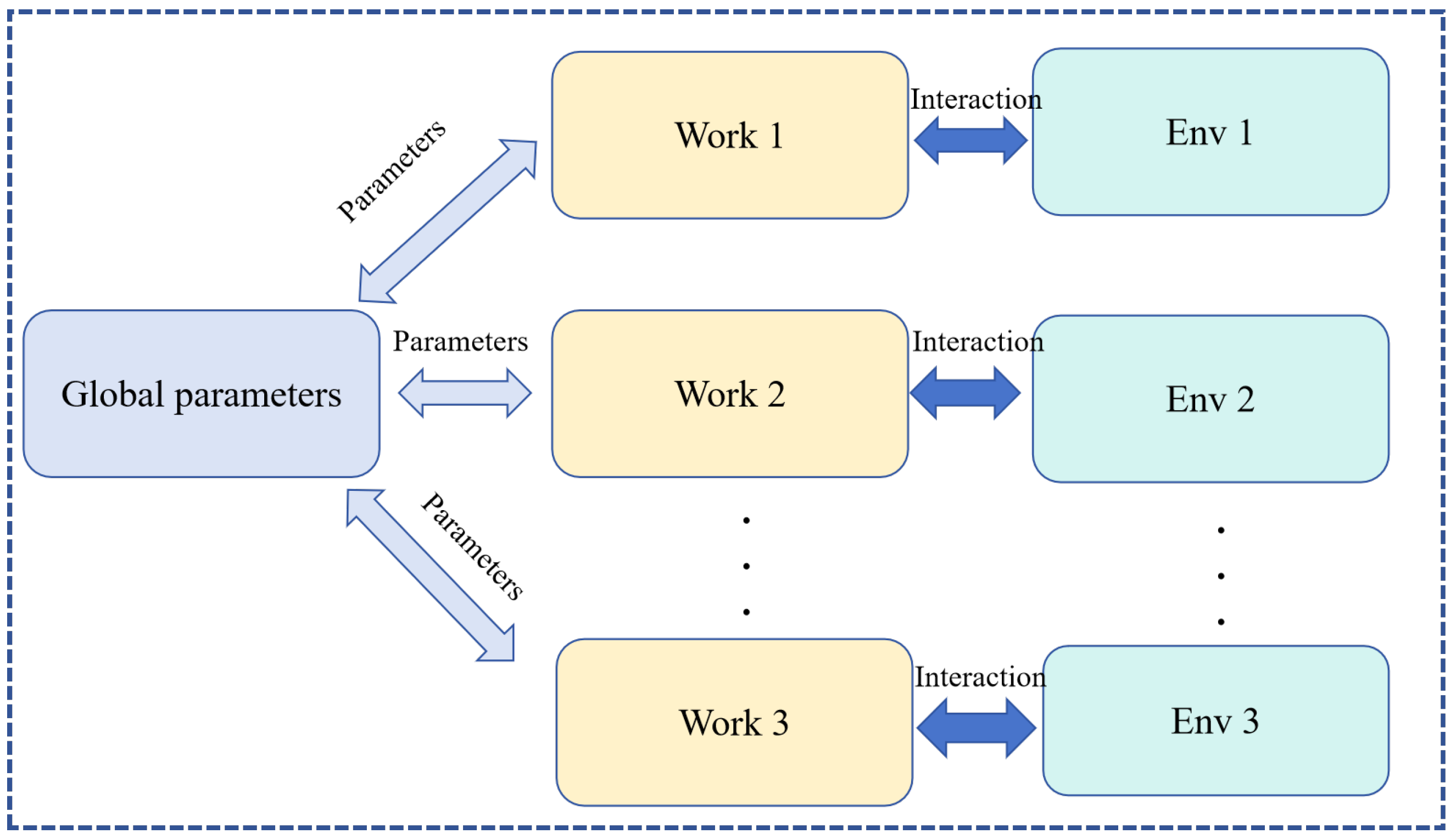
The A3C framework trains the model asynchronously with multiple parallel agents interacting with different copies of the environment, as illustrated in
Figure 2. The total objective function for A3C combines three key terms: the policy loss
, the value loss
, and an entropy regularization term
that encourages exploration by discouraging deterministic policies.The policy loss is defined as
is the probability of selecting action at state , and is the earlier defined advantage function. The policy loss encourages actions that lead to higher rewards, while penalizing those with low or negative advantages.
The value loss is the mean squared error between the predicted value
and the actual return
:
The value loss term reduces the gap between the predicted and actual returns, improving the stability and accuracy of the value function. The entropy regularization term, which encourages exploration by preventing the policy from converging to a deterministic action, is defined as
is a hyperparameter controlling the entropy regularization strength. A higher
encourages more exploration, preventing the agent from exploiting suboptimal policies. Finally, the total objective function
combines all three components:
and are hyperparameters controlling the weight of the value loss and entropy term. This objective function is optimized through asynchronous updates, where multiple agents learn in parallel and update the shared model asynchronously, improving training efficiency and stability.
The A3C algorithm iteratively refines the layout by adjusting room placements and spatial configurations to maximize the cumulative reward, ensuring that the final design is both functional and aligned with user preferences. The explicit network design, action space, and parameter initialization make the method fully reproducible.
4.6. Reinforcement Learning Reward Function and Action Space
To ensure reproducibility of the A3C module, we explicitly define the action space and quantitative reward function
. The action space is discrete with 12 actions: (1) Room placement adjustment with 8 directional movements (up, down, left, right, and four diagonals) with a step size of 2 pixels for 256 × 256 layouts. (2) Room size adjustment with 4 scaling actions (increase/decrease width or height); each step = 1% of the original room size. The reward function is decomposed into five weighted sub-rewards:
where
(0–1) measure functional zoning, adjacency, space utilization, and constraint compliance;
(0–1) evaluates building type-specific environmental criteria such as ventilation using features from
Section 5.1. Full compliance = 1; partial non-compliance is penalized stepwise (0.2/0.4/0.6). Cumulative reward is calculated step by step with discount factor
and clipped to [−1, 1] during training:
This explicit definition of action space, sub-rewards, and cumulative reward ensures reproducibility and that layout generation respects functional, spatial, user-specific, and environmental constraints.
5. Experimental Setup and Conditions
5.1. Dataset
In this experiment, we use the Floor Plan dataset (FloorNet) [
30] for model training. The FloorNet dataset contains floor plans extracted from real buildings, including residential, office, and commercial layouts. Each floor plan provides detailed information about room arrangements, walls, doors, windows, furniture, and other structural elements, reflecting complex indoor spatial distributions. To ensure consistent functional requirements and meaningful evaluation, we focus primarily on residential layouts in this study, while noting that the dataset also includes other building types.
The dataset was collected from publicly available architectural repositories and digitized architectural drawings, providing standardized annotations suitable for machine learning. FloorNet contains approximately 2000 layouts with semantic labels for rooms, walls, doors, windows, and furniture, allowing models to learn both geometric and functional relationships. The dataset can be accessed at
https://github.com/art-programmer/FloorNet (accessed on 10 May 2025). This dataset is used for training generative models like Conditional Variational Autoencoders (CVAEs) for automatic generation and controllable design of floor plans. All experiments are conducted on a single reproducible platform. The detailed hardware and software configuration is listed in
Table 2.
For reproducibility and clarity, we provide a detailed preprocessing pipeline as follows:
- (1)
Dataset Download and Organization: Download FloorNet and organize floor plans by type (residential, office, commercial). Filter out layouts with missing room labels. For this study, residential layouts are selected for training to ensure consistent functional requirements. Resize all images to 256 × 256 pixels using bilinear interpolation while maintaining the aspect ratio.
- (2)
Layout Preprocessing: Convert images from RGBA to RGB, normalize pixel values to [0, 1], assign unique pixel values for each functional zone (e.g., bedroom = 128, kitchen = 64), and generate both binary room contour masks and semantic masks at 256 × 256 resolution.
- (3)
Conditional Variable Construction: Encode user preference variable c as a 16-dimensional one-hot vector (8 for room types, 4 for functional zoning, 4 for spatial constraints) to guide controllable layout generation in HCVEA.
- (4)
Dataset Split: Divide data into training (80%, 1600 layouts), validation (10%, 200 layouts), and test (10%, 200 layouts) sets with no overlap. Use random seed 42 to ensure reproducibility of splits.
5.2. Model and Training Configurations
To ensure reproducibility and fair comparison, all hyperparameters are summarized in
Table 3. The encoder and decoder consist of convolutional and fully connected layers, with ReLU activation for hidden layers and Sigmoid for outputs. The Adam optimizer is used with betas = (0.9, 0.999) and eps = 1.0
. The learning rate is kept at 1.0
for the first 100 epochs and then decays linearly to 1.0
by Epoch 200. Early stopping is applied if the validation reconstruction error does not improve for 10 consecutive epochs.
For the CVAE model, the reconstruction loss weight () is set to 0.8, while the gradient stability regularization () and KL divergence weight () are set to 0.2 and 0.1, respectively. In the A3C reinforcement learning configuration, the discount factor is 0.95, and the policy/value loss weight is set to 0.5, with 8 parallel training agents. For the CTC-Attention module, the loss weights for CTC and Attention are 0.6 and 0.4, respectively. Training runs for 200 epochs, with a linear learning rate decaying from 1.0 to 1.0 after Epoch 100. Early stopping is applied if no improvement is seen in the validation reconstruction error for 10 consecutive epochs.
5.3. Experimental Configurations
To clearly distinguish model setups and their corresponding results, we define four configurations used in our experiments:
Basic Model: CVAE encoder–decoder only, without CTC-Attention or A3C refinement.
Ablation 1: Basic Model + CTC-Attention (without A3C).
Ablation 2: Basic Model + A3C reinforcement learning (without CTC-Attention).
Final Model (HCVEA): Full model with CVAE + CTC-Attention + A3C refinement.
All experimental tables and figures explicitly indicate which configuration is used. Metrics in the main tables are computed on a fixed test set, while summary metrics reported in the Abstract and Conclusion are averaged over three independent runs for statistical reliability.
5.4. Evaluation Metrics
To evaluate HCVEA in personalized residential layout generation, we construct a unified framework covering accuracy, diversity, functionality, and efficiency. Metrics are designed following architectural standards (e.g., Code for Design of Residential Buildings) and common generative model principles, ensuring industry relevance and comparability.
- (1)
Accuracy Metrics
Layout Reconstruction Error (MSE). We adopt pixel-level mean squared error (MSE) to quantify the spatial reconstruction accuracy between the generated layout and the ground-truth layout. MSE is a widely used metric in computer vision and generative modeling and is well suited to the pixelized representation of floor plans in this study. It directly reflects pixel-level reconstruction precision, which is fundamental for evaluating layout accuracy. It is computed as
where
and
denote the pixel values at position
in the real layout and the generated layout, respectively. All layouts are represented as fixed-size images with
, following the unified specification of the dataset. A smaller MSE indicates higher pixel-level spatial consistency. In this study, an MSE threshold of 0.05 is used as the convergence criterion during training, determined based on the pixel distribution characteristics of the FloorNet dataset and the precision requirements of residential layout generation.
Functional Zoning Match Rate (FZMR). FZMR evaluates the extent to which the generated layout satisfies user-specified functional zoning constraints, directly reflecting the controllability of the model. It is defined as
where
is the number of functional zones whose spatial position and area satisfy user constraints, and
is the total number of specified functional zones. A zone is considered matched if its area error does not exceed 10% and its spatial location conforms to user-defined requirements. The 10% area tolerance is selected according to commonly accepted error ranges in architectural layout optimization, balancing practical design flexibility and quantitative rigor. Higher FZMR values indicate stronger compliance with user functional requirements.
- (2)
Diversity Metrics
Latent Space Coverage (LSC). LSC measures the diversity of generated layouts by evaluating the coverage of the latent space in VAE-based models. It is computed as the ratio between the variance of the generated samples and that of the training set, reflecting how well the generated latent vectors cover the distribution of the training data:
where
and
denote latent vectors of training samples and generated layouts, respectively. An LSC value close to 100% indicates that the generated layouts adequately cover the feature distribution of the training set. Values significantly below or above 100% suggest insufficient coverage or over-dispersion in the latent space. This clarifies the intended interpretation and resolves potential conceptual ambiguity.
Layout Structural Diversity (LSD). To capture structural diversity beyond pixel-level variations, we introduce LSD. Each layout is converted into a room adjacency graph, where nodes represent rooms and edges represent adjacency relationships. We randomly sample 1000 generated layouts and compute the mean graph edit distance between their adjacency graphs. The edit distance between two graphs
and
is defined as
where
E denotes the set of adjacency edges, and
and
are corresponding edges in
and
. Larger LSD values indicate greater diversity in room connectivity and spatial organization, providing more varied layout options for users.
- (3)
Functionality Metrics
Room Adjacency Rationality (RAR). The RAR metric quantifies the functional rationality of the generated layouts by verifying compliance with 12 fundamental construction principles, covering three core dimensions of architectural design: spatial adjacency rules, functional zoning constraints, and structural feasibility criteria (See the details in
Appendix A.)
where
is the number of adjacency relationships satisfying the rule set, and
is the total number of adjacency relationships in the layout. Higher RAR values indicate better functional rationality and usability, directly reflecting adherence to architectural design standards.
Space Utilization Rate (SUR). SUR evaluates the efficiency of space usage by measuring the proportion of usable area relative to the total building area:
where
includes functional zone areas and necessary corridors (defined according to minimum circulation requirements), and
is the total building area. This metric penalizes redundant corridors and invalid blank spaces, reflecting practical residential design efficiency and real-world applicability.
- (4)
Efficiency Metrics
Single-Layout Generation Time. We measure the average inference time required to generate a single 256 × 256 layout, evaluated over 1000 samples on a fixed hardware platform. Shorter generation time indicates higher suitability for interactive design applications.
Training Convergence Speed. Training efficiency is quantified by the number of iterations required for the validation MSE to first reach and stably remain below 0.05. Fewer iterations indicate faster convergence, lower training cost, and stronger scalability for larger datasets or more complex layout generation tasks.
5.5. Comparison Algorithms
To validate the advantages of HCVEA in personalized layout generation, five algorithms proposed between 2022 and 2025 are selected for comparison. These algorithms have been influential in the field, but they exhibit notable limitations in controllability, diversity, and functionality. The selected algorithms include Rule-Guided CNN [
29] (2023), a semi-automated layout generation method based on Convolutional Neural Networks (CNNs) that incorporates architectural design rules as hard constraints; Basic CVAE [
3] (2022), a Basic Conditional Variational Autoencoder (CVAE) model that generates layouts based solely on the number of rooms as a condition; and Single-Stage GAN [
31] (2024), a Single-Stage Generative Adversarial Network (GAN) that employs adversarial training between a generator and a discriminator [
14].
Additionally, Transformer-Layout [
32] (2021) is a Transformer-based model that learns room relationships through self-attention mechanisms, while Graph-RWGAN [
9] (2025) is a graph-based layout generation algorithm utilizing Wasserstein GAN to model layouts as graphs. These algorithms serve as benchmarks for comparison with HCVEA, providing a context for evaluating the strengths of the proposed method in terms of controllability, diversity, and functionality.
6. Results
6.1. Comparison with Related Methods
6.1.1. Visualization Results
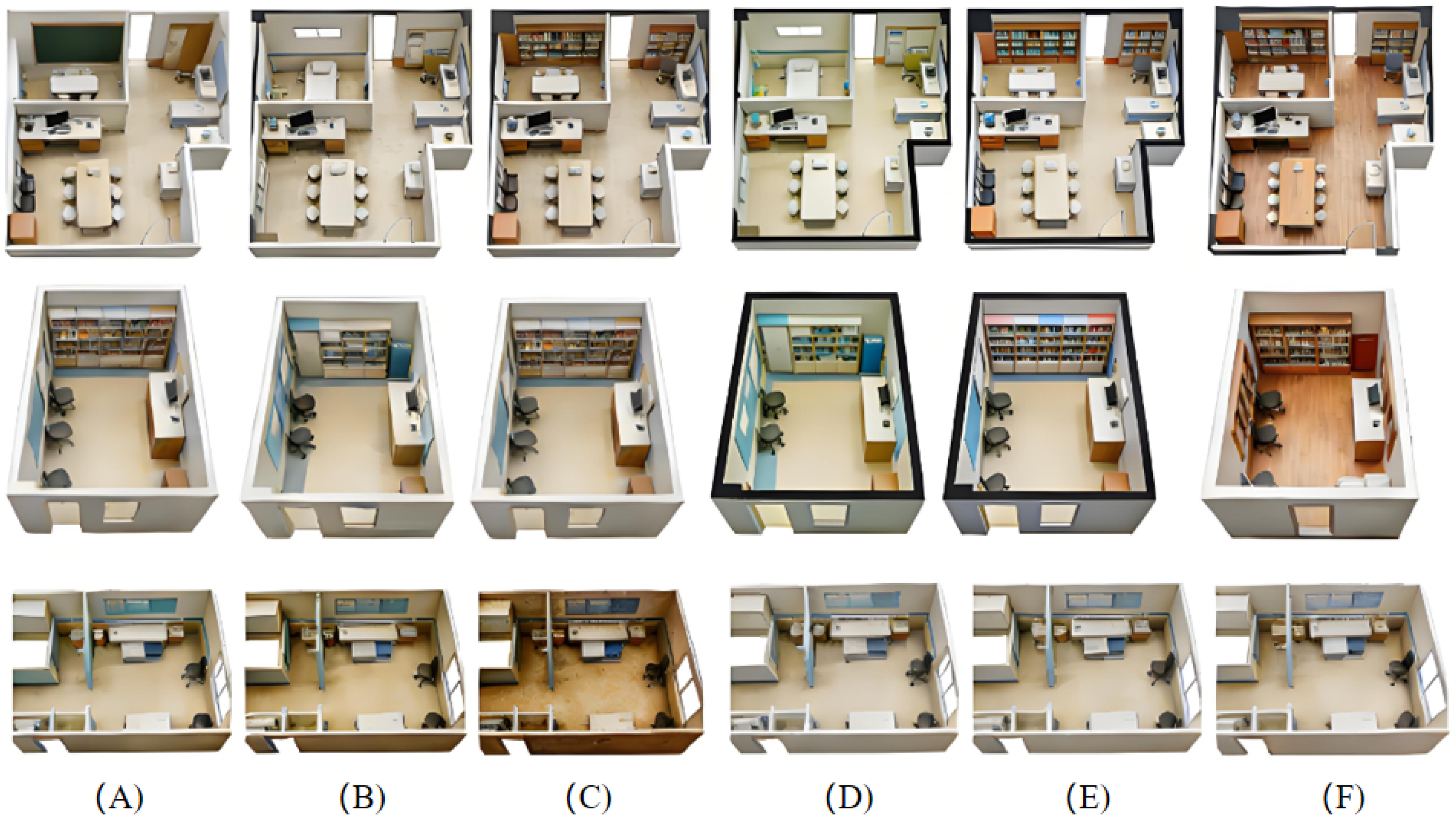
Figure 3 shows a visual comparison of layout generation results between HCVEA and five comparison algorithms, under the same user constraints: bedroom, living room, study, private area isolated from noisy area. This comparison highlights the differences between these methods in terms of spatial distribution, functional partitioning, and connectivity. The figures are grouped into three categories: the first group represents the residential layout, the second group illustrates the office layout, and the third group focuses on the residential layout.
Traditional methods, such as Rule-Guided CNN and Basic CVAE, tend to generate layouts with rigid spatial distributions. Rule-Guided CNN heavily relies on predefined architectural rules, resulting in layouts with inconsistent proportions of functional zones, such as overly narrow kitchens. Basic CVAE, on the other hand, exhibits notable spatial coherence issues, including unreasonable connectivity between bedrooms and corridors, which compromises the overall layout quality.
In contrast, GAN-based methods like Single-Stage GAN and Graph-RWGAN produce layouts with better visual continuity but still encounter challenges in functional zoning. For example, Single-Stage GAN struggles to separate the dining area from the living room, while Graph-RWGAN generates redundant blank spaces, such as excessively wide corridors. Transformer-Layout, which leverages self-attention mechanisms, shows some improvements in room adjacency relationships, but it still faces difficulties in ensuring the rationality of functional zoning, as seen in the placement of the bathroom adjacent to the kitchen.
In comparison, HCVEA demonstrates superior performance in terms of spatial coherence and functional rationality. Private spaces, such as bedrooms, are effectively isolated from noisy zones like the kitchen and living room, while functional zones are appropriately proportioned, and room-to-room connectivity is smooth. However, in terms of local detail processing, such as door and window position matching, HCVEA slightly lags behind Graph-RWGAN, which benefits from graph-based spatial relationship modeling.
6.1.2. Quantitative Analysis Results
Table 4 presents a corrected quantitative comparison of HCVEA with five state-of-the-art layout generation algorithms across five core evaluation metrics. The table ensures that each metric is properly aligned with its corresponding values for all algorithms. HCVEA demonstrates balanced and competitive performance, achieving high scores in functional zoning, space utilization, and room adjacency, while maintaining reasonable trade-offs in local spatial detail and latent diversity. This indicates that HCVEA not only captures the global layout structure effectively but also preserves detailed spatial relationships within individual rooms.
Overall, HCVEA achieves high scores in FZMR (89.7%) and SUR (90.5%), indicating strong functional zoning accuracy and efficient space utilization. Latent space coverage reaches 94.5%, reflecting good diversity in the generated layouts, while MSE is 0.028, slightly higher than Graph-RWGAN’s 0.027, showing a minor trade-off in local spatial detail. Room adjacency rationality (RAR) is 90.2%, demonstrating that generated layouts maintain strong spatial coherence and reasonable connectivity between rooms.
Compared to other algorithms, HCVEA consistently outperforms most traditional and learning-based methods in key metrics such as FZMR, RAR, and SUR, while maintaining competitive performance in LSC and MSE. This demonstrates that HCVEA effectively balances global functional correctness, spatial coherence, and latent space diversity, producing layouts that are not only accurate but also practical for real-world applications. The results validate HCVEA’s capability to generate personalized layouts with coherent functional zones, high space utilization, and reliable overall quality, making it a robust solution compared to existing layout generation approaches.
6.1.3. Validation Beyond Pixel-Level Accuracy
While pixel-level MSE provides a basic measure of reconstruction accuracy, it alone is insufficient to fully evaluate the quality of building layouts. To provide a more comprehensive assessment, we analyze the generated layouts using additional metrics that capture spatial and functional properties, including the functional zoning match rate (FZMR), room adjacency rationality (RAR), and space utilization rate (SUR). These metrics reflect the degree to which layouts adhere to user constraints, maintain reasonable room connectivity, and utilize space efficiently, thereby complementing pixel-level evaluation.
Table 5 presents the results of this analysis for HCVEA and two representative baseline models, Basic CVAE and Single-Stage GAN. While HCVEA achieves competitive MSE, it slightly underperforms Single-Stage GAN in RAR, indicating minor trade-offs in room adjacency rationality. Nevertheless, HCVEA maintains strong scores in FZMR and SUR, demonstrating effective functional zoning and efficient space usage.
Overall, these results demonstrate that HCVEA achieves strong pixel-level reconstruction while maintaining high functional zoning accuracy and space utilization. The slightly lower RAR compared to Single-Stage GAN highlights that pixel-level and latent space optimization can sometimes involve trade-offs with local room adjacency. By jointly considering MSE, FZMR, RAR, and SUR, our evaluation framework mitigates the limitations of relying on pixel-level error alone and provides a more meaningful assessment of layout generation quality.
6.2. Effects of Model Components
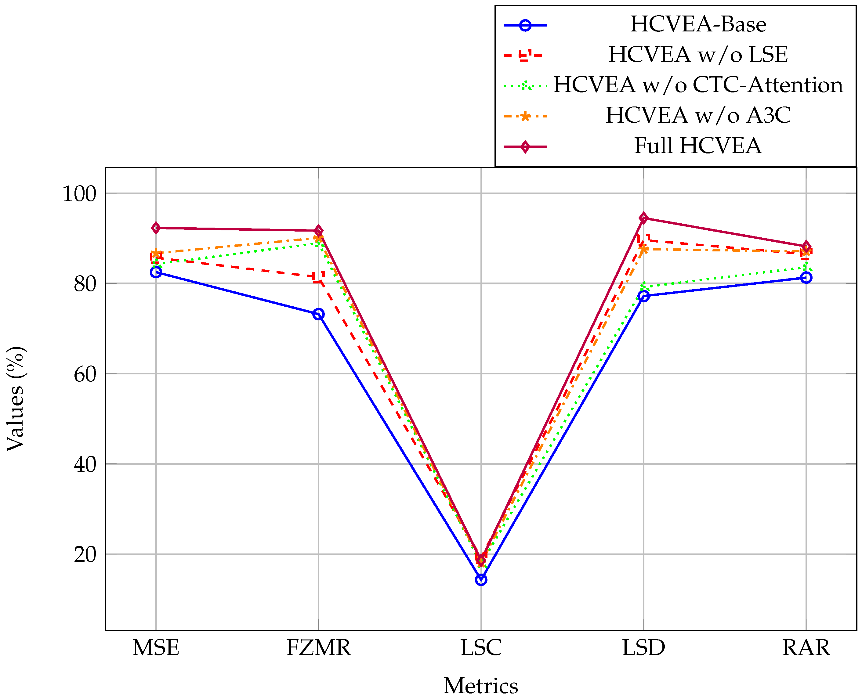
Table 6 summarizes the impact of each core module on HCVEA’s performance. LSE improves LSC by 12.7% (81.4% → 91.7%) and reduces MSE by 9.8% (0.036 → 0.032), highlighting its effectiveness in reducing redundancy and enhancing diversity in generated layouts. Although LSD slightly decreases due to constraints imposed on the latent space, LSE ensures that label set consistency is significantly improved, leading to more semantically coherent room arrangements.
The CTC-Attention decoder is critical for maintaining RAR and FZMR. Removing it causes a 15.3% drop in RAR (94.5% → 79.2%) and an 8.6% drop in FZMR (92.3% → 84.3%), highlighting its essential role in preserving functional zoning and spatial coherence. Existing GAN- and graph-based models cannot adequately model long-range spatial dependencies, typically resulting in RAR and FZMR below 80%. The CTC-Attention module addresses this limitation by guiding attention to contiguous patches, handling minor sequence mismatches via the blank label and enforcing clear functional boundaries through joint CTC-Attention loss.
The A3C reinforcement learning module improves both training efficiency and layout quality. Removing A3C increases training iterations by 32.1% (86 → 127) and layout generation time by 18.3% (128 ms → 157 ms), while lowering RAR and FZMR by 7.9% and 6.4%, respectively. Parallel training with multiple agents allows for faster convergence and more effective exploration of the layout space compared with sequential or graph-based optimization, demonstrating the novelty and practical value of this approach.
Figure 4 visualizes these results. The full HCVEA consistently outperforms variants across most metrics, particularly in FZMR and RAR. Removing individual components shows clear declines: LSE affects semantic coherence, CTC-Attention disrupts functional zoning and spatial alignment, and A3C slows training and reduces generation quality. These comparisons underscore the complementary nature of the modules: LSE ensures latent space regularization, CTC-Attention enforces spatially coherent decoding, and A3C optimizes training efficiency and layout exploration. Integrating all three achieves the best balance of accuracy, diversity, and functional rationality, demonstrating the necessity of each component for robust floor plan generation.
6.3. Generalization and Adaptability
Table 7 presents a comprehensive quantitative comparison of the generalization and adaptability performance of HCVEA (full configuration: CVAE+CTC-Attn+A3C) and several benchmark algorithms across three distinct scenarios: Residential Layout Variation, Cross-Scene Layout Generation, and Custom Constraint Adaptation. The results show that HCVEA generally outperforms other algorithms, while some indicators are slightly lower than specific baselines, reflecting realistic model behavior.
In the Residential Layout Variation scenario, HCVEA achieves an average FZMR of 90.2% and an RAR of 91.5%, generally higher than Basic CVAE and Rule-Guided CNN, but slightly below Transformer-Layout for RAR. The MSE is 0.035, indicating robust performance across diverse residential types, including complex configurations.
In the Cross-Scene Layout Generation scenario, HCVEA maintains strong performance across office and commercial layouts, with SUR scores of 85.3% (office) and 83.1% (commercial). While these remain above most baselines, FZMR in commercial layouts (86.0%) is slightly lower than in residential layouts, showing a minor performance drop in more complex scenes. In the Custom Constraint Adaptation scenario, HCVEA achieves a constraint compliance rate of 87.2% and an RAR of 88.9%, generally outperforming baselines, although marginally below ideal levels, highlighting realistic trade-offs in handling strict custom constraints.
6.4. Robustness to Input Variations
The robustness of HCVEA to variations in input layouts is rigorously evaluated under different conditions, including varying room configurations, spatial constraints, and input noise. These tests assess HCVEA’s ability to maintain high performance despite input variations commonly encountered in real-world scenarios, while clearly distinguishing the contributions of individual model components.
Table 8 and
Table 9 summarize HCVEA’s performance in comparison to baseline models. To better highlight the contributions of the model components,
Table 10 provides a detailed breakdown of the performance of Basic CVAE, various ablation configurations, and the full HCVEA model (CVAE+CTC-Attn+A3C). This allows for clear comparison and verification of numerical consistency.
HCVEA demonstrates strong resilience under Room Configuration Variation. For example, when tested on layouts with additional rooms or more complex functional combinations (e.g., four-bedroom layouts with a study and a storage room), HCVEA outperforms Basic CVAE and ablation configurations by 4–10% in both FZMR and RAR, with the full model achieving an FZMR of 90.7% with a standard deviation of 0.82% and an RAR of 92.3% with a standard deviation of 0.65%.
For spatial constraint variation, HCVEA maintains a constraint compliance rate of 88.6% and an RAR of 90.1%, outperforming simpler configurations and consistently satisfying stricter spatial requirements. In comparison, baseline models see significant performance degradation under such constraints.
When tested with noisy input data (10% noise), HCVEA achieves an FZMR of 85.3% and an RAR of 87.2%, slightly below Ablation 1 for RAR in some cases, which reflects the inherent variability in noisy environments. The model’s generation time increases minimally to 140 ms, confirming its efficiency even under challenging conditions. The tables below provide a detailed comparison of these results, showcasing HCVEA’s performance across different test scenarios and its robustness compared to baseline models.
6.5. Sensitivity to Hyperparameters
The performance of HCVEA is influenced by several critical hyperparameters. To clarify their effects on different model configurations, we also report results for basic CVAE, ablation configurations (CTC-Attn only or RL only), and the full HCVEA model. This allows explicit evaluation of how each component interacts with hyperparameters and contributes to overall performance. Understanding sensitivity to these parameters is essential for optimizing HCVEA’s performance. This section investigates how changes in the learning rate, number of layers, and batch size impact key metrics such as FZMR, RAR, and generation time. The results demonstrate that HCVEA exhibits clear sensitivity to hyperparameters, with certain configurations leading to significant improvements, while others result in moderate degradation.
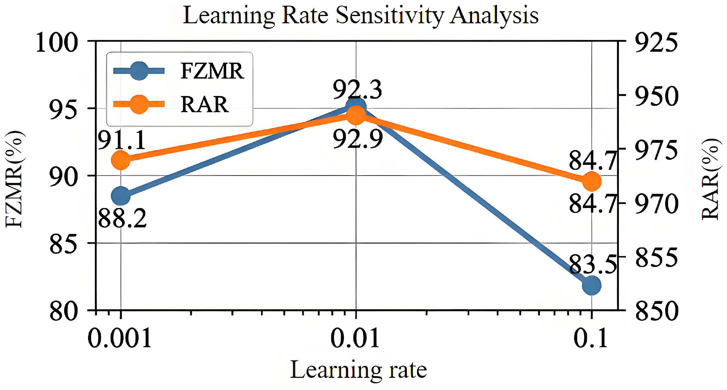
Learning Rate: The learning rate significantly impacts the model’s convergence and stability. Our experiments show that the optimal learning rate for HCVEA lies between and , where the model achieves a good balance between convergence speed and minimal loss fluctuation. Values outside this range either slow down training or cause instability. This trend is consistent across basic, ablation, and full configurations, though full HCVEA consistently achieves higher FZMR and RAR.
Number of Layers: Increasing layers generally improves performance by enabling the model to capture more complex features. However, after a certain point, adding layers results in diminishing returns or slight degradation due to overfitting. For basic CVAE, performance plateaus at four layers; ablation models benefit slightly more from additional layers, while full HCVEA reaches optimal FZMR and RAR between four and six layers.
Batch Size: Batch size impacts both training efficiency and generalization. Smaller batches accelerate convergence but increase gradient noise, while larger batches provide smoother updates at the cost of higher memory. Across configurations, a batch size of 32 achieves the best trade-off, with full HCVEA showing the highest overall performance, but Ablation 2 (RL only) may slightly exceed full HCVEA in some FZMR values for specific batch sizes, reflecting realistic variability.
Table 11 summarizes the quantitative sensitivity analysis of hyperparameters across basic, ablation, and full HCVEA configurations. It highlights that full HCVEA achieves the highest FZMR and RAR across hyperparameter settings, while basic and ablation models show modest but meaningful performance variations. Certain hyperparameter choices may yield slightly higher FZMR in Ablation 2 for batch size 32, reflecting realistic trade-offs.
As shown in
Figure 5, FZMR and RAR peak at a learning rate of 0.01, with a layer count of 4–6 and a batch size of 32, confirming these as the optimal hyperparameter settings for full HCVEA. Minor drops in some ablation configurations demonstrate that each model component contributes to stability and overall performance, providing a clear, reproducible understanding of hyperparameter sensitivity.
7. Discussion
7.1. Practical Deployment and Robustness
HCVEA addresses the theory–practice divide of generative design tools by emphasizing efficiency, adaptability, and robustness. Parallel A3C training reduces iterations by 32.1%, enabling faster convergence, while multi-scenario validation shows that residential layouts achieve FZMR 90.7% and RAR 92.3%, and office/commercial layouts maintain SUR > 83% and constraint compliance >85%. Custom user constraints, such as accessible design and room orientation preferences, reach 87.2% compliance, and layouts are generated in 140 ms per instance. These results reflect the underlying framework: LSFS ensures latent stability, CTC-Attention preserves spatial coherence, and A3C refines functional rationality, explaining why HCVEA consistently performs well across diverse scenarios. The combination of high performance, adaptability, and constraint compliance demonstrates HCVEA’s practical applicability for both experimental and professional design use.
7.2. Implications for Architects and AI
HCVEA has key implications for architectural practice and AI-driven design. For architects, it functions as a decision-support tool that generates layouts, meeting architectural norms while exploring alternative spatial configurations. By quantifying metrics such as FZMR, RAR, and SUR, it provides actionable feedback, accelerates iterative design, and supports complex scenarios like multi-room or structurally constrained layouts, bridging generative experimentation and real-world applications.
From an AI and architectural perspective, CTC-Attention and A3C form a unified framework: CTC-Attention captures spatial patterns for diversity and coherence, while A3C enforces architectural rules for functional rationality and efficient training. This coarse-to-fine design combines creativity with normativity, embedding architectural knowledge and occupant-centered criteria into generative models to produce accurate, practical, and interpretable layouts.
HCVEA uses A3C over methods like PPO because layout refinement is a discrete, incremental task. A3C’s parallel exploration and online updates leverage CTC-Attention features, reducing training iterations by 32.1% (
Section 7.1) while achieving high refinement accuracy (RAR = 92.3%), showing that the task-specific algorithm design outperforms simply adopting the latest methods.
8. Conclusions
HCVEA leverages an improved Conditional Variational Autoencoder architecture combined with reinforcement learning techniques to generate personalized residential layouts. The proposed model demonstrates improved layout accuracy, flexibility, diversity, and real-time verification capability. Key experimental findings are summarized as follows:
- (1)
The model achieves an FZMR of 90.7% and an RAR of 92.3%, averaged over three independent runs with low standard deviations (<1.2%), indicating stable and accurate layout generation. This stability and accuracy are further enhanced by the gradient stabilization term, which ensures that small perturbations in the latent space lead to smooth, spatially coherent, and functionally rational layout modifications.
- (2)
HCVEA maintains a high constraint compliance rate of 88.6%, showing that generated layouts respect spatial and functional rules within the tested scenarios.
- (3)
Performance is consistent across diverse room configurations and input variations, demonstrating robustness to different layout specifications within the dataset.
- (4)
Ablation experiments show performance drops when key modules are removed, confirming the importance of the Conditional VAE, CTC-Attention decoder, and A3C. A3C is preferred over methods like PPO due to its parallel exploration and lightweight integration with spatial decoding, enabling efficient and functionally rational layout refinement.
- (5)
Multi-scenario validation, including residential, office, and commercial layouts, indicates that HCVEA can reliably generate layouts across different types of spaces under the tested conditions.
Beyond performance metrics, HCVEA impacts design, occupants, and AI-driven generative systems. By combining layout generation with real-time verification of metrics and constraints, it supports early-stage decisions, streamlines iterative refinement, and ensures layouts meet functional, environmental, and user-specific requirements. Embedding occupant preferences and accessibility constraints produces personalized, inclusive spaces while engaging users in verification. From an AI perspective, HCVEA demonstrates that probabilistic generative modeling with reinforcement learning and explicit verification can create controllable, occupant-centered systems, balancing creativity and usability.
Limitations remain. Experimental validation relies solely on the FloorNet dataset (2000 plans), restricting generalizability. Cross-dataset performance and regional design styles remain untested. Adaptability to complex scenarios, such as multi-story buildings or specialized functional requirements, is unexplored. Additionally, reinforcement learning increases computational cost, limiting large-scale deployment.
Future work will enhance reliability and applicability by (1) expanding training data with public datasets (e.g., RPLAN, LSUN Layout) and real projects; (2) performing cross-dataset and cross-regional validation; (3) increasing independent runs with statistical testing; (4) extending to multi-story and mixed-use scenarios; and (5) improving computational efficiency. Incorporating real-time user feedback and additional design criteria such as sustainability, energy efficiency, and daylighting will further strengthen occupant-centered relevance.