1. Introduction
From the time of Euclid (300 BC) onwards builders and surveyors and the like have found the three-dimensional (3D) world in which they function to be adequately described by the theorems of Euclidean geometry. The shortest path between two points is a straight line, parallel lines never meet, the square on the hypotenuse equals the sum of squares on the other two sides, and so forth. When we look at the world about us we see a 3D world populated with 3D objects of various shapes and sizes. However, it is easy to show that what we see is a distorted or warped version of the Euclidean world that is actually out there. Hold the left and right index fingers close together about 10 cm in front of the eyes. They appear to be the same size. Fix the gaze on the right finger and move it out to arm’s length. The right finger now looks smaller than the left while, with the gaze fixed on the right finger, the left finger looks blurred and double. If the left finger is moved from side to side, neither of the double images occludes the smaller right finger; both images of the left finger appear transparent. The same phenomenon occurs regardless of which direction along the line of gaze the right finger is moved. Clearly, our binocular perception of 3D visual space is a distorted or warped version of the 3D Euclidean space actually out there.
Van Lier [
1], in his thesis on visual perception in golf putting, reviewed many studies indicating that the perceived visual space is a warped version of the actual world. He likened this to the distorted image of the world reflected in a sphere as depicted in M C Escher’s 1935 lithograph “
hand with reflecting sphere”. In Escher’s warped reflection straight lines have become curved, parallel lines are no longer parallel, and lengths and directions are altered. The exact nature of this warping can be defined by Riemannian geometry where the constant curvature of the sphere can be computed from the known Riemannian metric on a sphere. We mention Escher’s reflecting sphere simply to illustrate how the image of the 3D Euclidean world can be warped by the curvature of visual space. We are not claiming that the warped image of the Euclidean environment seen by humans is the same as a reflection in a sphere; indeed it is unlikely to be so. Nevertheless it provides a fitting analogy to introduce the Riemannian concept.
Luneburg [
2] appears to have been first to argue that the geometry of the perceived visual space is best described as Riemannian with constant negative curvature. He showed that the geometry of any manifold can be derived from its metric which suggested that the problem is “
to establish a metric for the manifold of visual sensation”. This is the approach we adopt here. We contend that the appropriate metric is that defined by the
size–distance relationship introduced by the geometrical optics of the eye, as will be detailed later in this section. It is due to this relationship that objects are perceived to change in size without changing their infinitesimal shape as they recede along the line of gaze. A small ball, for example, appears to shrink in size as it recedes but it still looks like a ball. It does not appear to distort into an ellipsoid or a cube or any other shape. This gives an important clue to the geometry of 3D perceived visual space. For objects to appear to shrink in size without changing their infinitesimal shape as they recede along the line of gaze, the 3D perceived visual space has to shrink equally in all three dimensions as a function of Euclidean distance along the line of gaze. If it did not behave in this way objects would appear to shrink in size unequally in their perceived width, height and depth dimensions and, consequently, not only their size but also their infinitesimal shape would appear to change. (We use the term “infinitesimal shape” because, as explained in
Section 4.1, differential shrinking in all three dimensions as a function of Euclidean distance causes a contraction in the perceived depth direction and so distorts the perceived shape of macroscopic objects in the depth direction as described by Gilinsky [
3].)
The perceived change in size of objects causes profound distortion. Perceived depths, lengths, areas, volumes, angles, velocities and accelerations all are transformed from their true values. It is those transformations that are encapsulated in the metric from which we can define the warping of perceived visual space. The terms “perceived visual space” and “perceived visual manifold” occur throughout this paper and, since in Riemannian geometry a manifold is simply a special type of topological space, we apply these terms synonymously. Moreover, the use of “perceived” should be interpreted philosophically from the point of view of indirect realism as opposed to direct realism, something we touch on in
Section 8. In other words, in our conceptualization, perceived visual space and the perceived visual manifold are expressions of the neural processing and mapping that form the physical representation of visual perception in the brain.
Since at least the eighteenth century, philosophers, artists and scientists have theorized on the nature of perceived visual space and various geometries have been proposed [
4,
5]. Beyond the simple demonstration above there has long been a wealth of formal experimental evidence to demonstrate that what we perceive is a warped transformation of physical space [
2,
3,
6,
7,
8,
9,
10,
11,
12,
13,
14]. In some cases a Riemannian model has seemed appropriate but, as we shall see from recent considerations, the mathematics of the distorted transformation is currently thought to depend on the experiment. Prominent in the field has been the work of Koenderink and colleagues, who were first to make direct measurements of the curvature of the horizontal plane in perceived visual space using the novel method of
exocentric pointing [
15,
16,
17]. Results showed large errors in the direction of pointing that varied systematically from veridical, depending on the exocentric locations of the pointer and the target. The curvature of the horizontal plane derived from these data revealed that the horizontal plane in perceived visual space is positively curved in the near zone and negatively curved in the far zone. Using alternative tasks requiring judgements of
parallelity [
18] and
collinearity [
19] this same group further measured the warping of the horizontal plane in perceived visual space. Results from the collinearity experiment were similar to those from the previous exocentric pointing experiment but, compared with the parallelity results, the deviations from veridical had a different pattern of variation and were much smaller.
Using the parallelity data, Cuijpers et al. [
20] derived the Riemannian metric and the Christoffel symbols for the perceived horizontal plane. They found that the Riemannian metric for the horizontal plane was
conformal, that is, the angles between vectors defined by the metric are equal to the angles defined by a Euclidean metric. They computed the components
of the curvature tensor and found them to be zero (i.e., flat) for every point in the horizontal plane. This was not consistent with their finding of both positive and negative curvature in the earlier pointing experiment. Meanwhile, despite the similarity of the experimental setups, these authors had concluded that their collinearity results could not be described by the same Riemannian geometry that applied to their parallelity results [
19]. The implication was that the geometry of the perceived visual space is task-dependent. From the continued work of this group [
21,
22,
23,
24,
25,
26,
27,
28,
29,
30,
31] along with that of other researchers, it is now apparent that experimental measures of the geometry of perceived visual space are not just task-dependent. They vary according to the many contextual factors that affect the spatial judgements that provide those measures [
4,
5,
32]. Along with the nature of the task these can include what is contained in the visual stimuli, the availability of external reference frames, the setting (indoors vs. outdoors), cue conditions, judgement methods, instructions, observer variables such as age, and the presence of illusions.
The inconsistency of results in the many attempts to measure perceptual visual space has led some to question or even abandon the concept of such a space [
19,
33]. This is unnecessary. Wagner and Gambino [
4] draw attention to researchers who argue that there really is only one visual space in our perceptual experience but that it has a cognitive overlay in which observers supplement perception with their knowledge of how distance affects size [
11,
34,
35,
36,
37,
38,
39]. We agree. However, Wagner [
32] argues that separation into sensory and cognitive components is meaningless unless the sensory component is reportable under some experimental condition. While there is, unfortunately, no unambiguous way to determine such a condition, mathematical models and simulations of sensory processes may provide a possible way around the dilemma. Rather than rejecting the existence of a geometrically invariant perceived visual space we suggest that the various measured geometries are accounted for by top-down cognitive mechanisms perturbing the underlying invariant geometry derivable mathematically from the size–distance relationship between the size of the image on the retina and the Euclidean distance between the nodal point of the eye and the object in the environment. This relationship is attributable to the anatomy of the human eye functioning as an optical system. For simplicity in what follows we will refer to this size–distance relationship as being attributable to the geometric optics of the eye. We now consider what determines that geometry.
The human visual system has evolved to take advantage of a frontal-looking, high-acuity central (foveal), low-acuity peripheral, binocular anatomy but at the same time it has had to cope with the inevitable size–distance relationship of retinal images that the geometric optics of such eyes impose. To allow survival in a changing and uncertain 3D Euclidean environment it would seem important for the visual system to have evolved so that the perceived 3D visual space matches as closely as possible the Euclidean structure of the actual 3D world. We contend that in order to achieve this, the visual system has to model the ever-present warping introduced by the geometrical optics of the eye and that this warping can be described by an invariant Riemannian geometry. Accordingly, this paper focuses on that geometry and on the way it can be incorporated into a realistic neural substrate.
A simple pinhole camera model of the human eye [
40,
41] shows that the size of the image on the retina of an object in the environment changes in inverse proportion to the Euclidean distance between the pinhole and the object in the environment. Modern schematic models of the eye are far more complex, with multiple refracting surfaces needed to emulate a full range of optical characteristics. However, as set out by Katz and Kruger [
42], object–image relationships can be determined by simple calculations using the optics of the reduced human eye due to Listing. They state:
[Listing] reduced the eye model to a single refracting surface, the vertex of which corresponds to the principal plane and the nodal point of which lies at the centre of curvature. The justification for this model is that the two principal points that lie midway in the anterior chamber are separated only by a fraction of a millimetre and hardly shift during accommodation. Similarly, the two nodal points lie equally close together and remain fixed near the posterior surface of the lens. In the reduced model the two principal points and the two nodal points are combined into a single principal point and a single nodal point. Retinal image sizes may be determined very easily because the nodal point is at the centre of curvature of this single refractory surface. A ray from the tip of an object directed toward the nodal point will go straight to the retina without bending, therefore object and image subtend the same angle. The retinal image size is found by multiplying the distance from the nodal point to the retina (17.2 mm) by the angle in radians subtended by the object [
42] (see Figure 18).
Thus the geometry of the eye determines that the size of the retinal image varies in proportion to the angle subtended by the object at the nodal point of the eye. Or stated equivalently, the geometry of the eye determines that the size of the image changes in inverse proportion to the Euclidean distance between the object and the nodal point of the eye. For the perceived sizes of objects in the perceived 3D visual space to change in inverse proportion to Euclidean distance along the line of gaze in the outside world without changing their perceived infinitesimal shape, the perceived 3D visual space has to shrink by equal amounts in all three dimensions in inverse proportion to the Euclidean distance. From this assertion, the Riemannian metric for the 3D perceived visual space can be deduced, and from the metric the geometry of the 3D perceived visual space can be computed and compared with the geometry measured experimentally.
Our principal aim is to present a mathematical theory of the information processing required within the human brain to account for the ability to form 3D images of the outside world as we move about within that world. As such, the theory developed is about the computational processes and not about the neural circuits that implement those computations. Nevertheless, the theory builds on established knowledge of the visual cortex (
Section 2) as well as on the existence of
place maps that have been shown to exist in hippocampal and parahippocampal regions of the brain [
43,
44,
45,
46,
47,
48,
49,
50]. Throughout this paper we take it as given that the
place and
orientation of the head, measured with respect to an external Cartesian reference frame (X,Y,Z), are encoded by neural activity in hippocampal and parahippocampal regions of the brain and that this region acts as a portal into visuospatial memory. We focus on the computational processes required within the brain to form a cognitive model of the 3D visual world experienced when moving about within that world. In that sense, the resulting Riemannian theory can be seen as an extension of the view-based theory of spatial representation in human vision proposed by Glennerster and colleagues [
51].
The theory is presented in a series of steps starting in the periphery and moving centrally as described in
Section 2 through
Section 7. To provide a road map and to illustrate how the various sections relate to each other, we provide here a brief overview.
Section 2: It is well known that images on the retinas are encoded into neural activity by photoreceptors and transmitted via retinal ganglion cells and cells in the lateral geniculate nuclei to cortical columns (hypercolumns) in the primary visual cortex. We define left and right retinal hyperfields and hypercolumns and describe the retinotopic connections between them. We treat hyperfields and hypercolumns as basic modules of image processing. We describe extraction of orthogonal features of images on corresponding left and right retinal hyperfields during each interval of fixed gaze by minicolumns within each hypercolumn. We further describe how the coordinates of image points in the 3D environment projecting on to left and right retinal hyperfields can be computed stereoscopically and encoded within each hypercolumn.
Section 3: Here we describe a means of accumulating an overall image of the environment seen from a fixed place. This depends on visual scanning of the environment via a sequence of fixed gaze points. We argue that at the end of each interval of fixed gaze, before the gaze is shifted and the information within the hypercolumns lost, the vectors of corresponding left and right retinal hyperfield image features encoded within each hypercolumn are pasted into a visuospatial gaze-based association memory network (
G-memory) in association with their cyclopean coordinates. The resulting gaze-based
G-memory forms an internal representation of the perceived 3D outside world with each ‘memory site’ accessed by the cyclopean coordinates of the corresponding image point in the 3D outside world. The 3D
G-space with image-point vectors stored in vector-spaces at each image point in the
G-space has the structure of a
vector bundle in Riemannian (or affine) geometry. We also contend in
Section 3 that the nervous system can adaptively model the
size–distance relationship between the size of the 2D retinal image on the fovea and the Euclidean distance in the outside world between the eye and the object. From this relationship the
Riemannian metric describing the perceived size of an object at each image point
in the environment can be deduced and stored at the corresponding image point
in
-memory. The
G-memory is then represented geometrically as a 3D Riemannian manifold (
,) with metric tensor field
. The geometry of the 3D perceived visual manifold can be computed from the way the metric
varies from image point to image point in the manifold.
Section 4: Applying the metric deduced in
Section 3, we use Riemannian geometry to quantify the warped geometry of the 3D perceived visual space.
Section 5: By simulating families of geodesic trajectories we illustrate the warping of the perceived visual space relative to the Euclidean world.
Section 6: Here we describe the computations involved in perceiving the size and shape of objects in the environment. When viewing from a fixed place, occlusions restrict us to seeing only curved 2D patches on the surfaces of 3D objects in the environment. The perceived 2D surfaces can be regarded as 2D submanifolds with boundary embedded in the ambient 3D perceived visual manifold (
,). We show how the size and shape of the submanifolds can be computed using Riemannian geometry. In particular, we compute the way the warped geometry of the 3D ambient perceived visual manifold (
,) causes the perceived size and shape of embedded surfaces to change as a function of position and orientation of the object in the environment relative to the observer.
Section 7: This introduces the notion of place-encoded visual images represented geometrically by a structure in Riemannian geometry known as a
fibre bundle. We propose that the place of the head in the environment, encoded by neural activity in the hippocampus, is represented geometrically as a point
in a 3D base manifold
called the
place map. Each point
in the base manifold
acts as an accession code for a partition of visuospatial memory (i.e., a vector bundle)
. As the person moves about in the local environment, the vectors of visual features acquired through visual scanning at each place
are stored into the vector bundle
accessed by the point (place)
in the base manifold
. Thus place-encoded images of the surfaces of objects as seen from different places in the environment are accumulated over time in different vector bundle partitions
of visuospatial memory. We show that adaptively tuned maps between each and every partition (vector bundle)
of visuospatial memory, known in Riemannian geometry as
vector-bundle morphisms, can remove occlusions and generate a 3D cognitive model of the local environment as seen in the correct perspective from any place in the environment.
Section 8: In this discussion section, material in the previous sections is pulled together and compared with experimental findings and with other theories of visuospatial representation.
Section 9: This section points to areas for future research development.
Riemannian geometry is concerned with curved spaces and the calculus of processes taking place within those curved spaces. This, we claim, is the best computational approach for analysis of visual processes within the curved geometry of 3D perceived visual space. A Riemannian geometry approach will reveal novel aspects of visual processing and allow the theory of 3D visual perception to be expressed in the language of modern mathematical physics. Our intention is to develop the groundwork for a theory of visual information processing able to account for the non-linearities and dynamics involved. The resulting theory will be integrated with our previous theory on the Riemannian geometry of human movement [
52] but in this paper we focus entirely on vision. We do not attempt to justify in a rigorous fashion the theorems and propositions that we draw from Riemannian geometry. For that we rely on several excellent texts on the subject and we direct readers to these at the appropriate places. However, for those unfamiliar with the mathematics involved, we have sought to provide intuitive descriptions of the geometrical concepts. We trust that these, together with similar descriptions in our previous paper [
52], can assist in making the power and the elegance of this remarkable geometry accessible to an interdisciplinary readership.
3. The Three-Dimensional Perceived Visual Space
The size–distance relationship introduced into retinal images by the optics of the eye is independent of the scene being viewed and of the position of the head in the environment. While the retinal image itself changes from one viewpoint to another, the geometry of the 3D perceived visual space derived from stereoscopic vision with estimates of Euclidean depth based on triangulation remains the same regardless of the scene and of the place of the head in the environment. In this section we present theory that describes a means for the visual system to form an internal representation of the 3D perceived visual space and of the visual images in that space viewed from a fixed place.
3.1. Gaze-Based Visuospatial Memory
When the head is in a fixed place and gaze is shifted from one gaze point to another the vector fields
VL and
VR of image-point vectors
and
over the hypercolumns described in
Section 2.10 are replaced by new image-point vectors and by new vector fields associated with the next gaze point in the scanning sequence. To build a visuospatial memory of an environment through scanning we argue that the information encoded by the vector fields
VL and
VR during a current interval of fixed gaze must be stored before the gaze is shifted and the information lost. Such memory is accumulated over time and scanning of an environment from a fixed place does not have to occur in one continuous sequence. Images associated with different gaze points from a fixed place can be acquired (and if necessary overwritten) in a piecemeal fashion every time the person passes through that given place.
We propose that, at the end of each interval of fixed gaze, the 30-dimensional image-point vectors
encoding left-hyperfield images within each hypercolumn are stored into a
gaze-based association memory or
-memory in association with their cyclopean coordinates
. Similarly, the 30-dimensional image-point vectors
encoding right-hyperfield images within each hypercolumn are stored in the same
-memory in association with their cyclopean coordinates
. In other words, the cyclopean coordinates
for each point ‘
’ in the 3D Euclidean outside space provides an
accession code for the
-memory. This concept of an accession code for memory stems from an earlier proposal of ours (see [
83] Section 8.3) and is analogous to the way the accession code in a library catalogue points to a book in the library. A particular cyclopean coordinate
gives the ‘site’ in the
-memory where two 30-dimensional image-point vectors
and
are stored. Actually, such a ‘site’ in an association memory network is distributed across the synapses of a large number of neurons in the network and the information is retrieved by activating the network with an associated pattern of neural activity encoding the cyclopean coordinate
, as in a Kohonen association neural network (see [
83] for further description).
The ‘library accession code’ analogy provides a simplified metaphor for the storage and retrieval of information in an association memory network and is used throughout the rest of the paper. Each site in the
-memory corresponds to a cyclopean image point
in the Euclidean environment. As shown in
Appendix A the left and right hyperfield image-point vectors
and
extrapolated from the same image point
in the outside space require 30 components (features) to adequately encode the non-linear stochastic characteristics of images on the hyperfields during each interval of fixed gaze. Thus each memory site can be thought of geometrically as a 30-dimensional vector space able to store two 30-dimensional image-point vectors. Because of disparity between left and right retinal images, the two 30-dimensional image-point vectors
and
stored at the image-point site
in the
-memory derive from different locations on the left and right retinas and are encoded within different hypercolumns. Thus, the storage of individual left and right image-point vectors
and
into the
-memory in association with their respective cyclopean coordinates
and
performs the task of linking disparate sites on left and right retinas receiving an image from the same image point in the environment.
For a fixed gaze point , the left and right image-point vectors associated with foveal hyperfields are fused by the gaze control system into a single hyperfield image-point vector. However, as the point in the environment moves away from the fixed gaze point , the difference between the left and right image-point vectors and increases because the size of retinal hyperfields and the densities of rods and cones change with retinal eccentricity. The superimposed left and right hyperfield images stored at the same site in the -memory become less well fused and, consequently, appear more fuzzy.
We define the
functional region of central vision to be an area containing all those points
in the Euclidean environment where the fuzziness and imprecision of location of the superimposed left and right hyperfield images
and
stored at the same site
in
-memory is acceptable for the visual task at hand. The size of this region varies with the visual resolution required for the particular task and with the Euclidean depth of gaze
. It varies with the extent of cluttering in the peripheral visual field [
82]. Points
in peripheral visual fields where the image-point vectors
and
stored at the same site
in
-memory are so different they cannot be fused into a single vector, give rise to the perception of double images, one from the left eye and one from the right eye, that may appear fuzzy.
As gaze is shifted from one point in the environment to another, large regions of the peripheral visual fields for the various gaze points overlap. Consequently, the sites in -memory where the peripheral image-point vectors associated with a current point of fixed gaze are to be stored may overlap with sites where image-point vectors associated with previous gaze points are already stored. We propose the following rule for determining whether or not image-point vectors already stored in -memory are overwritten by the image-point vectors associated with the current gaze point: Image-point vectors at sites in the peripheral visual field are only overwritten if the absolute difference between the left and right image-point vectors already stored at the site is larger than the absolute difference between the two image-point vectors for the same site associated with the current gaze point. Using this rule, the images accumulated in -memory from any given scanning pattern will consist of those image points that are closest to their regions of functional vision. As the number of gaze points in the scanning pattern increases, the above rule causes the acuity of the accumulated peripheral image to improve. In the extreme case, with an infinite number of gaze points in the scanning pattern, gaze is shifted to every point in the environment and only fused foveal images are stored at every site in an infinite -memory.
This is consistent with the evidence reviewed by Hulleman and Olivers [
107] showing that it is the fixation of gaze that is the fundamental unit underlying the way the cognitive system scans the visual environment for relevant information. The finer the detail required in the search task, the smaller the functional region of central vision and the greater the number of fixations required. The notion of a variable functional region of central vision provides a link between visual attention and peripheral vision and attributes a more important role to peripheral vision as argued by Rosenholtz [
82].
3.2. A Riemannian Metric for the G-Memory
As indicated in
Section 1, the size of the 2D image on the retina varies in inverse proportion to the Euclidean distance between the nodal point of the eye and the object. A key proposal of the present theory is that the nervous system can model adaptively the relationship between the Euclidean distance to an object in the outside world (sensed by triangulation) and the size of its image on the retina. The notion that this modelling is adaptive is consistent with the observation that the visual system can adapt to growth of the eye and to wearing multifocal glasses. We hypothesize that the modelled size–distance relationship can be applied to three dimensions and encoded in the form of a Riemannian metric
stored at every site
in the 3D cyclopean
-memory (for simplicity here and in what follows we have dropped the subscript
for peripheral points). In other words, we hypothesize that
the perceived size of a 3D object in the outside world varies in inverse proportion to the cyclopean Euclidean distance between the egocentre and the object, this being simply a reflection of the 2D size–distance relationship introduced by the optics of the eye.
When the -memory is endowed with the metric it can be represented geometrically as a Riemannian manifold (,). At each point in the (,) manifold there exists a 3D tangent space spanned by coordinate basis vectors . Any tangential velocity vector in the tangent space can be expressed as a linear combination of the coordinate basis vectors spanning that space. The metric inner product of any two vectors and in the tangent vector space at the point is denoted by and the angle between the two vectors is computed using . When the angle between the two vectors is rad the two vectors are said to be -orthogonal. We use this terminology throughout the paper.
The metric distance between any two points and in the (,) manifold is obtained by integrating the metric speed (i.e., metric norm or -norm ) of the tangential velocity vector along the geodesic path connecting the two points. This provides the visual system with a type of measure that can be used to compute distances, lengths and sizes in the perceived visual manifold (,). Since the metric changes from point to point in the manifold, and the metric speed depends on the metric, it follows that the metric distance between any two points and depends on where those points are located in the (,) manifold. In other words, the metric stretches or compresses (warps) the perceived visual manifold relative to the 3D Euclidean outside space.
In discussing the perception of objects, Frisby and Stone [
40] suggest that it would be helpful to dispense with the confusing term
size constancy and instead concentrate on the issue of the nature and function of the size representations that are built by our visual system. In keeping with this, we propose that, consistent with the size–distance relationship introduced by the optics of the eye,
the Riemannian metric on the perceived visual manifold varies inversely with the square of the cyclopean Euclidean distance and is independent of the cyclopean direction . This causes metric distances between neighbouring points in the perceived visual manifold (
,) to vary in all three dimensions in inverse proportion to cyclopean Euclidean distance
in the outside world. As a result, the perceived size of 3D objects in the outside world varies in inverse proportion to the cyclopean Euclidean distance
without changing their perceived infinitesimal shape. We use the term “infinitesimal shape” because, in attempting to define and establish a measure of subjective distance, Gilinsky states that “the depth dimension becomes perceptively compressed at greater distances” [
3] (p. 463). Consequently, as a macroscopic object recedes its shape appears to change because its contraction is greater in the depth extent than in height or width.
The proposal that the Riemannian metric (r) varies only as a function of cyclopean Euclidean distance and is independent of cyclopean direction implies that the metric is constant on concentric spheres in the outside world centred on the egocentre. These concentric spheres play an important role in describing the geometry of the perceived visual manifold and from now on we refer to them simply as the visual spheres.
For the size of an object to be perceived as changing in all three dimensions in inverse proportion to the cyclopean Euclidean distance without changing its infinitesimal shape, the Riemannian metric (r) must be such that the -norm of the tangential velocity vector at each point in the perceived visual manifold is equal to the norm of the velocity vector in Euclidean space (where is the metric of the 3D Euclidean space) divided by the cyclopean Euclidean distance , that is, at each point.
If egocentric Cartesian coordinates
are employed, the Euclidean metric for the outside world is:
and the required Riemannian metric
for the perceived visual manifold (
,g) is:
That is,
However, the depth and direction of gaze is best described using spherical coordinates
. Thus we require the Riemannian metric of the perceived visual manifold to be expressed in terms of
. The transformation between spherical coordinates
and Cartesian coordinates
in Euclidean space is given by:
When the Euclidean metric in Equation (1) is pulled back to spherical coordinates using Equation (4) we get:
Consequently, the Riemannian metric
for the perceived visual manifold is:
That is,
where:
In Euclidean space, using spherical coordinates, tangential velocities are related to angular velocities by:
If the inverses of the relationships in Equation (9) are used to express the angular velocities (
in terms of the tangential velocities (
, then the terms
and
in Equation (5) cancel and we obtain:
In other words, to compute the norm of the Euclidean tangential velocity vector
in Euclidean spherical coordinates we require the Euclidean metric:
Thus the Riemannian metric matrix required to compute the
-norm
of the tangential velocity vector
at any point
in the perceived visual manifold
is:
4. Quantifying the Geometry of the Perceived Visual Manifold
Given the metric in Equation (7) and/or Equation (12) depending on the coordinates employed, the theorems of Riemannian geometry can be applied to compute measures of the warping of the perceived visual manifold . In this section we use the geometry to quantify: (i) the relation between perceived depth and Euclidean distance in the outside world; (ii) the illusory accelerations associated with an object moving at constant speed in a straight line in the outside world; (iii) the perceived curvatures and accelerations of lines in the outside world; (iv) the curved accelerating trajectories (geodesic trajectories) in the outside world perceived as constant speed straight lines; (v) the Christoffel symbols describing the change of coordinate basis vectors from point to point in the perceived visual manifold; and (vi) the curvature at every point in the perceived visual manifold. Together, these Riemannian measures provide a detailed quantitative description of the warped geometry of the perceived visual manifold that can be compared with measures obtained experimentally.
4.1. The Relationship Between Perceived Depth and Euclidean Distance
As described by Lee [
57] (Chapter 3), two metrics
and
on a Riemannian manifold are said to be
conformal if there is a positive, real-valued, smooth function
on the manifold such that
. Two Riemannian manifolds
and
are said to be
conformally equivalent if there is a diffeomorphism (i.e., one-to-one, onto, smooth, invertible map)
between them such that the pull back
is conformal to
. Conformally equivalent manifolds have the same angles between tangent vectors at each point but the
-norms of the vectors are different and the lengths of curves and distances between points are different. Conformal mappings between conformally equivalent manifolds preserve both the angles and the infinitesimal shape of objects but not their size or curvature. For example, a conformal transformation of a Euclidean plane with Cartesian rectangular coordinates intersecting at right angles produces a compact plane with curvilinear coordinates that nevertheless still intersect at right angles [
108].
Let us now consider two spaces, one being corresponding to the Euclidean outside world with Euclidean metric (Equation (5)) and Euclidean distance and the other being corresponding to the perceived visual manifold with metric (Equations (7) or (12)) and metric distance . The Riemannian manifold is, by definition, locally Euclidean and can be mapped diffeomorphically to the Euclidean space . The symbol can be used, therefore, to represent both the distances from the origin in and from the egocentre in . We use this convention throughout the paper, however in this section (and only this section) we separate and because we are interested in the relationship between them. Comparing Equation (5) and Equation (7), it can be deduced that . This shows that the 3D Euclidean outside world and the 3D perceived visual manifold are conformally equivalent with conformal metrics and and with equalling the positive, smooth, real-valued function mentioned above.
Thus, from the theory of conformal geometry the following properties of the perceived visual manifold follow: (a) Objects appear to change in size in inverse proportion to the Euclidean distance
in the Euclidean outside world without changing their apparent infinitesimal shape. (b) The perceived visual manifold
is isotropic at the egocentre; i.e., the apparent change in size with Euclidean distance
is the same in all directions radiating out from the egocentric origin. (c) There exists a diffeomorphic map between the two manifolds but it does not preserve the metric; i.e., the map is not an isometry. While there is a one-to-one mapping between points in the outside space and points in the perceived visual manifold, the two spaces are not isometric so distances between points are not preserved. (d) Angles between vectors in corresponding tangent spaces
and
are preserved. (e) As the Euclidean distance
increases towards infinity in
the perceived distance
in
converges uniformly to a limit point. Stars in the night sky, for example, appear as dots of light in the dome of the sky. (f) If
is the Euclidean distance from
O to a point in
, the perceived distance
from
O to the corresponding point in
can be computed using Equation (2) by integrating the metric norm of the unit radial velocity vector
along the radial path to obtain:
The lower limit has been fixed to unity to remove ambiguity about the arbitrary constant of integration and, consequently, the integral is given by the following function of its upper limit:
as illustrated graphically in
Figure 3. The perceived distance
is foreshortened in all radial directions in the perceived visual manifold relative to the corresponding distance
in the Euclidean outside space. The amount of foreshortening increases with increasing
.
It is interesting to notice in
Figure 3 that according to the logarithmic relationship the perceived distance
is negative for values of
less than one. This does not immediately make intuitive sense because perceived distance should always be a positive number. In fact it implies an anomaly, the existence of a hole about the egocentric origin in
that cannot be perceived. This
does make intuitive sense because we cannot see our own head let alone our own ego. The existence of a hole at the origin has consequences for the perception of areas and volumes containing the origin, but we will not explore that further here.
4.2. The Geodesic Spray Field
As defined in Riemannian geometry [
109] (Chapter IV), the geodesic spray field,
is a second-order vector field in the double-tangent bundle
over the tangent bundle
at each point
in the perceived visual manifold
and at each velocity
in the tangent vector space
at
. The geodesic spray field is well known in Riemannian geometry and we have previously given a detailed description of it [
52]. At each point
in the manifold
, there exists a tangent space containing the velocity vector (or the direction vector)
, and at each point
in the tangent space, there exists a tangent space on the tangent space; that is, a double tangent space. The double tangent space contains the geodesic spray field. It is not a tensor field so it depends on the chosen coordinates and since it can be precomputed as described below it can be regarded as an inherent part of the perceived visual manifold
. It has two parts,
and
, known as the horizontal part and vertical part, respectively. The horizontal part
equals the tangential velocity
in the 3D tangent vector space
at each
. The vertical part
provides a measure of the
negative of the illusory acceleration perceived by a person looking at an object that is actually moving relatively in the outside world at constant speed (the negative sign is explained in the next section).
To illustrate, telegraph poles observed from a car moving at constant speed along a straight road appear not only to loom in size but also to accelerate as they approach. This common example shows that our perceptions of the position, velocity and acceleration of moving objects are distorted in ways consistent with the proposed warped geometry of the visual system. The illusory acceleration can be attributed to the metric in Equations (7) and (12) causing the apparent distance between neighbouring points in to appear to increase as the distance in the Euclidean outside world decreases. Consequently, an object appears to travel through greater distances per unit time as it gets closer to the observer and, therefore, appears to accelerate as it approaches.
The velocity at each is measured relative to the cyclopean coordinate basis vectors spanning the 3D tangent vector space . However, warping of the perceived visual manifold causes these basis vectors to change relative to each other from point to point in the manifold. As a result, since the velocity at each point is measured with respect to these basis vectors, their changes from point to point give rise to apparent changes in the velocity vector , thereby inducing illusory accelerations. These illusory accelerations do not happen in flat Euclidean space. The negative of the geodesic spray vector provides a measure of this illusory acceleration at each position and velocity in the tangent bundle (i.e., union of all the tangent spaces over ). The geodesic spray field on the tangent bundle can be precomputed and can, therefore, be regarded as an inherent part of the perceived visual manifold .
As shown by Lang [
109] and by Marsden and Ratiu [
110], the acceleration part
of the geodesic spray field is given by the equation:
where
represents the metric inner product,
is the Jacobian matrix of the metric
in Equation (7),
is a fixed arbitrary vector, and
.
Solving Equation (16) for
as a function of position and velocity on the perceived visual manifold
we obtain:
where (
) are the components of
in cyclopean spherical coordinates at each position
and velocity
in the tangent bundle
.
Since, as mentioned above, the geodesic spray field is non-tensorial it follows that it depends on the chosen coordinate basis vectors. When the components (
) of the acceleration geodesic spray field
in Equation (17) are recomputed in terms of the tangential velocities
,
, and
in Equation (9) and the metric
in Equation (12), we obtain a different expression:
The illusory accelerations introduced by the warped geometry of the perceived visual space are easier to understand intuitively when presented in terms of the tangential velocities
,
, and
in Equation (18). For example, if
,
, and
, corresponding to an object approaching the observer at constant unit speed along a radial line (like looking out the front window of a train travelling at constant speed along a straight line), the spray acceleration
equals a radial acceleration
directed outward along the radial line. The negative of this is consistent with the object appearing to accelerate as it approaches. If
,
, and
, corresponding to an object moving normal to the line of sight (like looking out a side window of the same train), the radial acceleration
given by Equation (18) equals the centripetal acceleration required for the object to follow a circular motion with constant tangential velocity centred about the egocentre (consistent with the perceived acceleration of an object seen from a side window of the train at a distance
normal to the train). If
,
, and
, corresponding to an object having both radial and tangential components of velocity (like looking ahead but off to one side from the front window of the train), the spray acceleration
given by Equation (18) has a radial component
and a tangential component
. The latter equals a coriolis acceleration causing a change in the rate of rotation of the coordinates or direction of gaze. These intuitive descriptions are verified in
Section 5 below.
4.3. Covariant Derivatives
Covariant derivatives defined in Riemannian geometry have an important role to play in visual perception. They provide a quantitative measure of the perceived directional accelerations of objects moving in the outside world taking both actual accelerations and illusory accelerations into account. They also quantify the perceived curvature at each point along the edges of objects and thereby provide the perceived shape of objects as judged from their outlines (see
Section 6). Importantly, the perceived rate of change in the nominated direction at the specified point is measured relative to the curvature of the ambient perceived visual manifold at that point. Given a curve
in the manifold
parameterized by time
the covariant derivative
of the velocity vector
tangent to the curve in the direction
at the point
is obtained by subtracting the spray acceleration
from the acceleration
at the point
:
The acceleration
is an ordinary Euclidean acceleration. It does not take into account rotation of the coordinate basis vectors
from point to point in the manifold, so does not include illusory accelerations. It can be interpreted as a measure of the actual Euclidean acceleration at the corresponding point and direction in the Euclidean outside world.
If the Euclidean acceleration
is everywhere zero (i.e., the object is moving at constant speed along a straight line in the environment) then we obtain:
at every point
along the curve. In this case the covariant derivative
is the perceived illusory acceleration equal to the negative of the geodesic spray vector
at each point
along the curve; i.e., the object appears to accelerate towards the observer as it approaches or decelerate as it recedes. If the Euclidean acceleration
is not zero and the object is actually accelerating in the Euclidean outside world (most likely following a curved path) then the covariant derivative in Equation (19) gives the perceived metric directional acceleration in the direction
at each point along the path, taking both the actual Euclidean acceleration and the illusory acceleration into account. It is important to notice that the covariant derivative can be used to measure the
perceived accelerations across the perceived visual manifold. We will use this fact in subsequent sections.
We can now ask the converse question. How does an object have to move in the Euclidean outside world for it to be perceived as moving at constant speed in a straight line? By setting the perceived acceleration
equal to zero in Equation (19) we obtain:
Thus, to be perceived as moving in a straight line at constant metric speed, an object in the Euclidean outside world has actually to be accelerating with a Euclidean acceleration
which, at every point along its path in Euclidean space, equals the acceleration spray vector
at the corresponding point and velocity in the perceived visual manifold
. In other words, to be perceived as moving in a straight line at constant speed the object must follow a (usually curved) path in the outside world with a Euclidean acceleration
equal but opposite in sign to the illusory acceleration
introduced by the visual system. This is exactly how the geodesics of the perceived visual manifold
are defined. The geodesics are accelerating curves in the Euclidean outside world that appear as straight lines with constant metric speed (i.e., their metric acceleration
equals zero) in the perceived visual manifold
.
The covariant derivative where X and are arbitrary vector fields on provides a measure at each point of the rate of change of the vector for movement in the X-direction. In other words, it measures the directional derivative of the vector in the X-direction taking into account the warping of the manifold and hence the illusory acceleration. We now use this definition of the covariant derivative to obtain a measure relating to the concept of parallelity. At each point along a geodesic there exists a vector tangent to the curve. The family of vectors forms a vector field along the geodesic . Being a geodesic, has zero metric acceleration (), hence is perceived as being a constant speed straight line while tangent vectors along it are perceived as being collinear and are said to be parallel translated along .
This notion of parallel translation can be generalized to any family of vectors
along
not necessarily tangent to the geodesic
. As presented by Lang [
109], the change in the vector
for movement in the direction
along
is given by the covariant derivative
where
is the Jacobian matrix of the vector
at each point
along the curve and
is a symmetrical bilinear map at
that transforms the two vectors
and
in the 3D tangent vector space
at the point
along the curve into an acceleration vector in
. The bilinear map
is algebraically related to the geodesic spray field
and, as shown in Equations (23) and (24), given one the other can be computed [
109]:
When the covariant derivative
in Equation (22) is zero everywhere along the curve
the vector
is said to be parallel translated along
and all the vectors
along the curve are parallel to each other. Parallel translation of the vector
at
to the vector
at
along
is path dependent and is described by
where
is a linear invertible isometric transformation between the vector spaces
and
along the curve.
Defined in this way, parallel transformation has a useful role to play in understanding visual perception. This is because vectors
that are parallel translated along a geodesic in the visual manifold will be perceived as being parallel to each other, whereas they are not parallel in the Euclidean outside world. The generalized covariant derivative
of vector field
along
and the associated parallel translation of
along
when
can be used to quantify the difference between lines in the outside world that are truly parallel and lines that are perceived as being parallel. This underlies the experimental work of Cuijpers and colleagues [
17,
18,
19,
20] introduced in
Section 1 and discussed in
Section 8.5.
4.4. Christoffel Symbols
To simplify notation in this section and the next we implement a number-indexing system that equates
r with 1,
with 2, and
with 3. Thus, for example, the cyclopean coordinate basis vectors
and
spanning a tangent vector space will be written in the alternative form
with
k = 1, 2, 3 and we introduce the
Christoffel symbols notated as
with
. The Christoffel symbols
are important in vision because they allow us to quantify the relative directional rates of change of the coordinate basis vectors
that occur with infinitesimal movements in the warped visual manifold
. They are related to the covariant derivatives
with
measuring the rate of change of each coordinate basis vector
associated with movement in the direction of another coordinate basis vector
at each point
in the manifold
. As indicated in
Section 4.2, it is this change in the coordinate basis vectors with movement across the manifold that gives rise to illusory accelerations of objects moving in the outside world. It should not be a surprise, therefore, that the Christoffel symbols provide an alternative way of quantifying the components
of the acceleration spray vector
at each position and velocity
. The repetition of the indices
and
first as superscripts and then as subscripts in this equation implies summation over
. Known as Einstein’s summation convention, it is used from here forward in this paper, particularly in
Section 4.5. There we introduce tensors which operate on dual spaces of vectors and covectors (analogously to matrices operating on dual spaces of column and row vectors). To facilitate use of the summation convention, index positions are always chosen so that vectors have lower indices and covectors have upper indices while the components of vectors have upper indices and those of covectors have lower indices. This ensures that the Einstein summation convention can always be applied. This simplifies notation by removing the need for summation signs. We require the Christoffel symbols in order to compute the Riemann curvature at each point in the manifold in
Section 4.5.
At each
, the Christoffel symbols
correspond to the components of the covariant derivative vector
in the tangent space projected on to the basis vectors spanning the tangent space at that point; that is:
Notice the use of the Einstein summation convention in the last term in Equation (25). Working in this way generates a large number of components
, i.e., 27 Christoffel symbols are required at each point
in the 3D perceived visual manifold
. Nevertheless, these have the advantage that they can be computed at each point from the known metric
and its differentials. By definition, in any Riemannian manifold the Christoffel symbols are compatible with the Riemannian metric, that is
, and are symmetrical, that is
. From these properties the following equation expressing the Christoffel symbols at each point in terms of the metric
and its differentials is derived [
111]:
where
are the components of
at each
and
are the components of the inverse metric
at each
.
Using Equation (26) and the Riemannian metric in Equation (12), we computed all 27 Christoffel symbols for the perceived visual manifold
as a function of their position
in
. We found all to be zero except for the following seven:
Returning to
notation, the subparts of Equation (27) show respectively:
(i) so only the component of in the direction is non-zero,
(ii) so only the component of in the direction is non-zero,
(iii) so only the component of in the direction is non-zero,
(iv and v) so only the components of in the direction are non-zero, and (vi and vii) so only the components of in the direction are non-zero. We now use this information to compute the curvature of the perceived visual manifold .
4.5. The Riemann Curvature Tensor
Warping of the perceived visual manifold is quantified by the Riemann curvature tensor at each point in the manifold. However, while the curvature of a 2D surface is an easily understood concept, the idea of the curvature of a 3D manifold is more difficult to grasp. Hence we provide the following intuitive description. A key property of the 3D Euclidean outside world is that it is “flat” with zero curvature everywhere. Consequently, an arbitrary tangent vector can be parallel translated along any pathway between any two points and remain parallel everywhere. In other words, in the Euclidean world parallel translation is path independent and the flat space is said to be totally parallel. Given arbitrary vector fields and on the flat Euclidean space, parallel translation of a vector for an infinitesimal time along the integral flow of followed by parallel translation for an infinitesimal time along the integral flow of does not in general equal parallel translation of the vector for an infinitesimal time along the integral flow of followed by parallel translation for an infinitesimal time along the integral flow of . Equivalently, in terms of covariant derivatives, , and we can say that in general the products of covariant derivatives do not commute, even on flat Euclidean spaces. However, by definition, equals , where is a vector known as the Lie bracket. Thus, for arbitrary vector fields and and an arbitrary vector on a flat Euclidean space, we can write that . This provides a criterion for flatness. Any other space for which does not equal zero is not flat. Indeed we can define a curvature operator that operates on a vector to give a vector at every point across a manifold. If is not zero at a point then the manifold is not flat at that point and the magnitude of the vector provides a measure of how far the curvature deviates from flatness.
Similar to the curvature operator
operating on a vector
across a manifold, we now define a
curvature tensor that quantifies curvature as a real number independently of the coordinates in which a manifold is expressed. Using the tensor characterization lemma [
57] (Chapter 2) and by introducing a covector
(i.e., a dual vector similar to a row vector in linear matrix theory) at each point in the manifold, we can define a type (1,3) curvature tensor that operates on three vectors
and a covector
and transforms them into a real number:
The vectors
can be written as linear combinations
,
,
of the cyclopean coordinate basis vectors
and
spanning the tangent space
at the point
and the covector
can be written as a linear combination
of the dual basis vectors
spanning the covector space
at
. Notice the use of upper and lower indices consistent with the Einstein summation convention (
Section 4.4). The tensor
can be represented as a tensor in an 81-dimensional tensor space spanned by basis tensors
(
signifies tensor product) with components
quantifying the projection onto each basis tensor. The tensor
can then be expressed in terms of its
components,
at each
. The components
can be computed [
111] from the previously obtained Christoffel symbols in Equation (27) using the equation:
Applying Equation (30), we computed all 81 components
of the curvature tensor
as a function of position
in
. We then implemented a useful conversion that entails expressing the tensor
in the form
where
is the vector in
dual to the covector
in
. The type (0,4) Riemann curvature tensor
can be represented as a tensor in an 81-dimensional tensor space spanned by basis tensors
with components
quantifying the projection onto each basis tensor. The Riemann curvature tensor
can then be expressed in terms of its
components,
at each
by the operation known as
lowering the index. This is achieved using the important property of Riemannian metrics
that allows us to convert tangent vectors to cotangent vectors and vice versa; viz.,
and
[
57] (Chapter 2). In terms of coordinate basis vectors
spanning the tangent space
at the point
and coordinate basis covectors
spanning the dual cotangent space
at the same point
this conversion can be written as
. In other words, the components convert according to
. This is called
lowering the index on the components. Applying this between components
and
of the curvature tensors gives:
where
from Equation (12). The advantage of lowering the index on the curvature components
in this way to obtain components
is that curvature components
are known to possess symmetries
,
,
, and
. These symmetries allow the number of components to be greatly reduced. Indeed, for the 81 components
computed using Equation (30) we find that all components
of the Riemann curvature tensor
at each point
are zero with the exception of the following three:
where
is the Euclidean cyclopean distance from the egocentre. As described in the next section, these three nonzero components of the Riemann curvature tensor are known as
sectional curvatures of
. In
Section 5 we examine these sectional curvatures by means of geodesic simulations.
6. Binocular Perception of the Size and Shape of Objects
When seen from a fixed place, the perceived surfaces of objects in the environment are represented geometrically by 2D curved surfaces with boundary (or surfaces with corners) isometrically embedded in the perceived visual manifold . The space between objects in the environment is transparent and so the perceived image-point vectors for points in the outside world between objects are zero vectors. Similarly, points in the environment occluded from view by other objects also have zero image-point vectors. Image points on embedded 2D surfaces are easily detected, therefore, because they are the only image points with non-zero image-point vectors. Image points on the boundaries (edges) of perceived 2D embedded surfaces are also easily detected because they correspond to points in where the image points and/or the image-point vectors change rapidly from a foreground to a background surface. In the case of a semi-transparent object there are two images, one from transmission through the object and the other a reflection from the semi-transparent object. Reflection causes the orientation of the image to reverse and the vector bundle is said to be twisted. Although reflections can be handled within Riemannian geometry we will not explore them further in this paper. In aerial perspective the atmosphere causes images of objects to become hazy with increasing distance. But still the image-point vectors of the hazy object do not become zero. Thus image-point vectors of embedded surfaces, including reflecting surfaces, are easily detected because they are the only points in with non-zero image-point vectors.
We will use the notation
to represent a 2D submanifold (surface) embedded in the 3D ambient perceived visual manifold
, and
to represent its boundary. As described in Riemannian geometry [
57] (Chapter 8), an isometric embedding of
into
is a smooth map (isometric embedding)
with the unknown metric
at each point on
induced by the pull back
of the known metric
on the ambient manifold. The smooth map
, and hence the metric
, depends on the shape of the object in the outside world and this shape is unknown. It follows that the pulled-back metric
and the shape of the embedded surface
have to be computed from the image-point vectors in the
-memory of
Section 3.
The unknown metric on a 2D embedded submanifold is different from the known metric at the same point in the ambient manifold , and its rate of change across the surface of the embedded submanifold is different from the rate of change of along the same path in the ambient manifold . The 2D embedded submanifold is perceived, therefore, as a 2D surface with boundary that is curved relative to the ambient 3D perceived visual manifold in which it is embedded. Computing the size and shape of embedded surfaces from image-point vectors stored in -memory is complicated by the fact that all perceived measures of the surface are made relative to the ambient perceived visual manifold and this ambient manifold is itself curved (warped) relative to the Euclidean outside world.
6.1. Seeing the Size of an Object
Consider measuring the size of an object in the outside world with a tape measure. The perceived size of both the object and the tape measure change with distance
in exactly the same way so the size of the object according to the measure given by the tape remains the same regardless of the distance
. Now consider the concept of a “perceptual tape measure”. By this we mean an internal reference metric that changes its infinitesimal length
as a function of
in exactly the same way as does the perceived image of an actual tape measure. The use of such an internal reference allows the actual size of an object to be determined regardless of its position in the scene. Since the metric
decreases smoothly as the distance
from the egocentre increases, it follows that the infinitesimal length
at a point along a curve
in
changes as the point on the curve moves closer or further away from the egocentre. Despite this differential expansion/contraction of the curve, a measure of its length
between any two points
and
along the curve is always obtainable by integrating its metric speed
along the curve between the points:
Given an internal reference metric that can be moved to any point in
, Equation (36) provides an implementation of a perceptual tape measure able to measure the actual size of perceived objects and distances between points in the outside world taking the warped geometry of the perceived visual space into account. In other words, Equation (36) allows the internal reference metric to change its length as a function of distance
r in
in exactly the same way the perception of an actual tape measure changes its length as a function of distance
r in the outside world. As put by Frisby and Stone, “[the object] looks both smaller and of the correct size given its position in the scene” [
40] (p. 41). The precision of a measurement made using a perceptual tape measure will decrease as the object being measured moves further away from the egocentre because of the reduced size of both the object and the perceptual tape. Incorrect estimates of Euclidean distance
will alter the differential stretching of the perceived curve and lead to misperceptions of both apparent and actual size as well as to other illusions (
Section 2.8 and
Section 8.4).
6.2. Seeing the Outline of an Object
The perceived shape of the boundary of a two-dimensional submanifold embedded in (or at least of those segments of the boundary that belong to the object and not to other occluding objects) plays an important role in object recognition. Sketching the outline of a hand, for example, provides sufficient information to recognize that the object is a hand. This is an interesting observation because both the perceived boundary and the perceived shape of the boundary of an object vary with the position and orientation of the object in the environment relative to the observer and are not invariant properties of the object. Actually, a smooth 3D object in the outside world does not have an edge and the perceived boundary corresponds to a curve on the surface of the 3D object (and in the ambient manifold) that varies depending on the position and orientation of the object relative to the observer. Nevertheless, when observed from a fixed place, objects in the environment have clearly perceivable boundaries or edges.
Cutting and Massironi [
112] and Cutting [
98] pointed out that many cave paintings, as well as cartoons, caricatures and doodles are made of lines and, as images, they depict objects well. They proposed a taxonomy of lines [
112], describing
edge lines that separate a figure from the background,
object lines where the line stands for an entire object in front of the background,
crack lines that imply an interior space hidden from view, and
texture lines that can represent small edges, small objects, small cracks as well as changes in shading and colour. They also pointed out that by using just a few well-crafted lines an artist can sketch the outline of partly occluded objects in such a way that both the occluding and the occluded objects can be recognized.
Despite the variety of line types, when looking at three-dimensional objects in the environment from a fixed place, lines are representations of the boundaries (or segments of boundaries) of perceived two-dimensional submanifolds embedded in the perceived visual manifold
. The perceived edge of the object is a curve (or segment of a curve)
embedded in the perceived visual manifold
. The perceived shape of the outline of the object is quantified by the perceived curvature
at each point
along the curve. As given by Lee [
57] for curves in Riemannian manifolds in general, the curvature
of a unit metric speed curve
at each point
along the curve is equal to the metric acceleration of the unit metric speed curve at that point.
As shown in
Section 4.3, the perceived acceleration of a point moving along a unit metric speed curve
in the ambient perceived visual manifold
is given by the covariant derivative
at each point
along the curve. Since the covariant derivative
is zero for a geodesic curve in
(geodesic curves appear as constant metric speed straight lines), it follows that the perceived curvature
provides a quantitative measure of how far the unit metric-speed boundary curve
deviates from a geodesic in the ambient manifold at each point along the curve. Thus, the perceived shape of the outline of an object is encoded by the perceived covariant derivatives
in the ambient manifold at each point
along the curve. The apparent curvature is perceived, therefore, relative to the inherent curvature of the ambient manifold at each point.
6.3 Seeing the Shape of an Object
As the gaze point
is moved about on the surface of an object in the environment, the perceived 2D surface
is described by a smooth function
between the Euclidean cyclopean distance
and the cyclopean direction
. Indeed, providing the point
on the surface
is within the functional region of central vision, the function
can be computed for the space about a single point of gaze. The partial derivatives
and
of this function at each point
on the surface define two vectors in the 3D ambient tangent space
at each point on the surface. The two vectors span a 2D subspace
in
that is tangent to the 2D submanifold
at the point
. Note that each point
on the submanifold is also a point
in the ambient manifold. The cross product
of these two vectors defines a vector
in
at each point
that is normal to the 2D submanifold
at each point
. The vector
at each point can be normalized to obtain a unit length vector
that spans the one-dimensional subspace
normal to the submanifold
at each point
. It follows from this that the second fundamental form
(defined in
Appendix B) is a vector normal to the surface in the normal bundle
at each point
that can be written as:
where
is a real number (scalar) equal to the metric length
of the vector
.
Thus (see
Appendix B) we can replace the vector-valued second fundamental form
with a simpler scalar-valued form
known as the
scalar second fundamental form. This acts on any two vectors
in
and transforms them into a real number
at every point
. Therefore, it is a symmetrical 2-covariant tensor field over the submanifold
. Using the index raising lemma and the tensor characterization lemma Lee [
57] (Chapter 8) shows that
can be expressed in the form:
where
is a linear, symmetrical, nonsingular, matrix operator, known as the
shape operator. It is a linear endomorphism that operates on any vector
in
and transforms it into another vector
in
. Because the shape operator
is a symmetrical matrix it has two orthonormal eigenvectors
and
in the tangent space
known as the
principal directions and two corresponding eigenvalues
and
known as the
principal curvatures of the submanifold
at the point
. In other words:
The principal curvature
equals the maximum curvature of the submanifold
at the point
in the principal direction
. The principal curvature
equals the minimum curvature of the submanifold
at the point
in the principal direction
.
In
Appendix B we show that the covariant derivative
provides measures of the perceived principal curvature
and the principal direction
of the submanifold at each point
. Likewise the covariant derivative
provides measures of the perceived principal curvature
and the principal direction
of the submanifold at each point
. Although the covariant derivative
is computed in the ambient manifold
, the vector
is contained in the 2D vector space
tangent to the submanifold at the point
. The principal direction vector
is easy to find, being the only vector in
for which the two vectors
and
in
are collinear. Because the shape operator
is a non-singular symmetrical matrix, eigenvector
is orthogonal to
so it too is easy to find. The metric length
of the covariant derivative vector
equals the maximum principal curvature
of the submanifold at the point
and the metric length
of the covariant derivative vector
equals the minimum principal curvature
of the submanifold at the same point. It makes intuitive sense that the rate at which the normal vector
rotates as the point
moves across the surface of the submanifold is related to the curvature of the submanifold. The more curved the submanifold, the greater the rate of rotation of the normal vector
.
Equation (A9) in
Appendix B shows that the perceived curvature at each point
on a submanifold
is equal to the product
of the principal curvatures at that point. However, the product
is equal to:
That is, the perceived curvature
equals the difference between the
Gaussian curvature of the submanifold
at the point
and the
sectional curvature of the ambient manifold
at the same point
.
The Gaussian curvature
of the submanifold depends on the unknown metric
induced on the submanifold by the embedding
and consequently, it is influenced by the actual shape of the object in the Euclidean outside world. However, the Gaussian curvature of the submanifold is not an intrinsic property of the object but varies with the position and orientation of the embedded submanifold
in the ambient perceived visual manifold
. This is contrary to Gauss’s famous
theorema egregium that asserts that the Gaussian curvature is an intrinsic property of the object, but that theorem only holds for submanifolds embedded in Euclidean spaces. Here we are considering a submanifold embedded in a curved ambient perceived visual space
. As shown in
Appendix B, the sectional curvature
of the ambient manifold
depends on the position
in the ambient manifold and on the orientation of the plane II in
spanned by the orthonormal eigenvectors
and
that are tangent to the submanifold at the point
. From this we see that, while the perceived shape of the 2D submanifold embedded in the perceived visual manifold
is influenced by the intrinsic shape of the object in the environment, it does not equal the intrinsic shape but varies as a function of the position and orientation of the object relative to the egocentre of the observer.
To show that the perceived curvature
at every point on the surface of an object seen from a fixed place is not sufficient to determine uniquely the perceived shape of the surface, consider the example of a cylinder embedded in Euclidean space. The maximum principal curvature
is measured in the direction
tangent to the circumference of the cylinder and the minimum principal curvature
is measured in the direction
tangent to the long axis of the cylinder. The minimum principal curvature
is zero everywhere along the long axis of the cylinder so the product
is zero at every point on the cylinder. But the cylinder has a different shape from the Euclidean plane for which the product
also equals zero. Thus, the product
is not sufficient to uniquely encode the local shape of the submanifold. As described by Trucco and Verri [
113] and illustrated in
Figure 9, it requires a combination of the mean
and the product
of the principal curvatures to encode the local shape uniquely.
7. A Geometric Representation of Visuospatial Memory
Thus far, we have described -memory as providing an internal representation of the egocentric 3D outside world viewed stereoscopically from a fixed place in that world. We have proposed that, during each interval of fixed gaze, the encoded left and right image-point vectors associated with each point in the environment are stored in -memory in association with their cyclopean coordinates . Thus, over time, through visual scanning of the environment from the fixed place, the -memory accumulates an image of the entire 3D environment as seen from that place. The warped geometry of the perceived visual space is encoded by the Riemannian metric stored at each site in the -memory. Thus the -memory encodes both the warped geometry of the perceived environment and the image of the environment as seen from the fixed place.
We now extend the model of -memory to include moving the head (egocentre) from place to place in the environment. The size–distance relationship introduced by the optics of the eye is unchanged by moving the head from place to place (and hence the metric is unchanged) but the retinal image does change because of changes in perspective associated with the different viewpoints. In this section, we first describe a geometric structure (known as a vector bundle) for -memory associated with a fixed place, and we then extend this to a geometric structure (known as a fibre bundle) to account for variable place. The extended geometric structure incorporates a partitioning of visuospatial memory into a family of sub-memories (or -memories) accessed by the hippocampal encoding of place. Thus the different sub-memories encode images of the environment seen from different places (i.e., place-encoded images). Finally, we describe a geometric mapping between sub-memories (known as a vector-bundle morphism) that can remove occlusions and turn visuospatial memory into a 3D cognitive model of the visual environment as seen from different places in that environment.
7.1. The Geometric Structure of G-Memory for a Fixed Place
As described in
Section 3, each site
in
-memory corresponds to a point in the 3D Euclidean outside world specified in cyclopean spherical coordinates relative to the egocentric place of the head in the environment (i.e., the egocentre). The
-memory can, therefore, be taken to be an internal representation of 3D egocentric perceived visual space. We now consider the geometric structure of that space. When each point
in the perceived visual manifold
is associated with image-point vectors
and
stored at that site, the structure takes on a geometric form illustrated in
Figure 10.
At each image point in the manifold there exists a fibre (i.e., a geometric fibre not a nerve fibre) containing a 30-dimensional vector space in which two 30-dimensional image-point vectors and are stored. The fibre includes both the image point and the vector space so the union of all the fibres over all points in equals the total space called a vector bundle .
A vector bundle is a well-known structure in Riemannian geometry. It consists of a pair of smooth spaces,
(the total space) and
(the base space), with a smooth surjective (onto) map
(the projection) between them [
57] (Chapter 2). The total space
is a smooth 33-dimensional manifold; three dimensions are required to specify the position
in
and 30 dimensions are required to specify each image-point vector
and
in the vector space
at
in
. A
section of
is a map
such that each
is an image-point vector (
or
) over its image point
. Each section
is thus a vector field made up of all the image-point vectors over all the points
in
acquired through visual scanning with the head in a fixed place. The vector space of all possible vector fields
over
) is depicted by the notation
(
Figure 10).
The vector fields
VL and
VR in
(consisting of all the left and right image-point vectors
and
over all the image-points
in
accumulated within a single vector bundle
through visual scanning) thus encode a visual image of the entire 3D environment as seen from the given fixed place. However, while we describe vector fields
VL and
VR as being defined over all image points
in
, it must be kept in mind from
Section 6 that the image-point vectors
and
are only non-zero at those points
that are located on the surfaces of objects. We also note again here that if the visual environment includes reflections then the orientation of the reflected images is reversed and the vector bundle is said to be twisted [
114].
An important geometric idea illustrated in
Figure 10 is the notion of open subsets
in
. An open subset
can be expanded or contracted to any size. It can even cover all of
. Vector fields
VL and
VR confined to open subsets
in
can be defined and all the fibres within these can be parallel processed as a unit. Indeed, it is this point processing (i.e., within fibre) nature of computations in Riemannian geometry that makes this geometry so well suited for describing parallel processing in the nervous system.
If images from a sufficiently large number of gaze points with the head in a fixed place are accumulated in the vector bundle
then, because of the rule for overwriting image-point vectors (
Section 3.1), the two vector fields
VL and
VR in
can be regarded as fused into a single binocular vector field
V over
. For simplicity of description, in subsequent sections we assume that a sufficient number of gaze points have been accumulated through visual scanning for the vector fields
VL and
VR in
to be fused into a single binocular vector field
V over
in the vector bundle
.
7.2. The Geometric Structure of Visuospatial Memory with Place Encoding
As a person moves from place to place in a local Euclidean environment the images of objects projected on to the retinas change according to changes in the perspective from which they are viewed. We propose that visuospatial memory is partitioned into sub-memories, each represented geometrically by a vector bundle
with
being an accession code corresponding to the place
of the head (egocentre) in the 3D Euclidean outside world. As indicated in
Section 1, it is well established that a place map
is neurally encoded in the hippocampus [
43,
44,
45,
46,
47,
48,
49,
50] and we see this as providing the place manifold
in what follows. Every time the person passes through a given place
in the environment, the retinal images, acquired from a sequence of fixed gaze points with the head in that place, are encoded and stored into the appropriate vector bundle sub-memory
associated with that place. The stored images are continuously updated through experience. Over time, many images of the environment acquired by visual scanning from different places in the environment are accumulated into the appropriate place-related vector bundle sub-memories. Since each vector bundle
is associated with a different place
, we refer to the images of the environment stored in different vector bundle sub-memories as
place-encoded visual images. The street-view feature of Google maps provides a useful analogy. The street address on the Google map is analogous to the place
of the head in the environment, while all the street-view images at that point on the Google map are analogous to all the images acquired by visual scanning at place
in the environment and stored in the vector bundle
associated with
.
Each vector bundle
corresponds to a
-memory representing the perceived visual manifold
associated with the place
.
Figure 11 depicts this schematically for two places
and
. In each vector bundle sub-memory
the Riemannian metric
and the warped geometry of the perceived visual manifold
are identical. In other words, image points
in any one sub-memory can be mapped to corresponding image points
in all other sub-memories and, because the warped geometries of all the
manifolds are identical, the flow of image points associated with moving the head from place to place (i.e.,
optical flow) can be represented by the flow of image points in a single equivalent
manifold.
As shown in
Figure 11, the place map
in the hippocampus is represented geometrically by a 3D base Euclidean manifold with a Cartesian external reference frame
. As the person moves about in the outside world, the movement is represented by a curve
, parameterized by time
, in the place manifold
. Since it is not possible to walk through a brick wall or to float up into the air, for example, it is not possible for the point
to move everywhere in the place manifold
. The existence of
no-go places forms a boundary
on the place manifold
. At each reachable point
in the 3D place manifold
, there exists a fibre containing a vector bundle
(i.e., a partition of visuospatial memory). Thus, each place
acts as an accession code for a vector bundle sub-memory
and each vector bundle sub-memory contains a place-encoded visual image of the environment associated with that place.
While the manifolds in the various vector bundles are geometrically equivalent with the same Riemannian metric field and hence the same warping, the image-point vectors and the vector fields stored in each -memory are different because, although they are images of the same environment, they have each been viewed from a different place in that environment. The changing perspective causes the embedded surfaces of objects in the environment to be stored at different sites in the various -memories and the embedded surfaces have different sizes, angles, and orientations depending on the place from where they were viewed. Image points occluded from view in one vector bundle are not occluded in others and vice versa. As we will see, it is the difference in the vector fields stored in the various -memories and the way they change from one vector bundle to the next that encodes information about the 3D structure of the outside world.
7.3. Fibre Bundles and Vector-Bundle Morphisms
Partitioning of visuospatial memory into vector-bundle sub-memories containing place-encoded visual images can be represented geometrically by a structure in Riemannian geometry known as a
fibre bundle, illustrated for two places
and
in the place manifold
in
Figure 11. Every point
in the place manifold, together with its associated vector bundle
, forms a fibre and the union of these fibres forms a fibre bundle. Notice that the definition of a fibre used here is different from that in
Section 7.1. Whereas a fibre in
Section 7.1 consisted of an image point
in
and the associated vector space
in the vector bundle
, the fibre defined here consists of a point
in the place manifold
and an entire vector bundle
, not just a vector space. This difference in the definition of the fibre defines the difference between the vector bundle and the fibre bundle.
The fibre bundle described does not provide a full 3D representation of the outside world. The vector field
stored in each vector bundle
encodes only the images of curved 2D embedded submanifolds (with boundaries) corresponding to visible patches on the surfaces of objects that can be seen from the fixed place. Theory exists within Riemannian geometry, however, describing maps between vector bundles known as
vector-bundle morphisms [
109,
114]. Vector-bundle morphisms allow the place-encoded images stored in the various vector bundles
to be mapped reciprocally on to each other. Image points
and their associated image-point vectors
in one vector bundle
at one point
in the base manifold
can be transformed by a vector-bundle morphism into the corresponding image points
and their associated image-point vectors
in another vector bundle
located at another point
in the base manifold
. Remember, images stored in different vector bundles are of the same environment but seen from different places in that environment and so are different because of differences in perspective. Vector-bundle morphisms can transform the image from any one vector bundle into every other vector bundle. In this way, vector-bundle morphisms can remove occlusions and generate 3D place-encoded images of the 3D outside world with the correct perspective for each place.
7.4. Removing Occlusions
To give a simplified illustration of how vector-bundle morphisms can remove occlusions (and generate 3D images), consider two photographs A and B of the same scene taken from different places in the environment. While it is quickly recognized that the photographs are of the same scene, closer scrutiny will reveal many differences between them. The same image points in the outside world are located at different places in the two photographs. Objects in the photographs may differ in size, the angles between them will be different and the outlines may vary in shape. While many image points in the scene are represented in both photographs, there are also many image points that can be seen in one photograph but are occluded from view in the other. There are also image points occluded from view in both photographs.
Let us define image points that can be seen in both photographs as image points; image points that can be seen in photograph A but not in photograph B as image points; image points that can be seen in photograph B but not in photograph A as image points; and image points that cannot be seen in either photograph as image points. In this simplified illustration, a vector-bundle morphism can be thought of as a map able to transform image points (i.e., a small matrix array of pixels depicting a small region of the scene, like the tip of a person’s nose) from photograph A to photograph B, and an inverse map able to transform image points in the reverse direction from photograph B to photograph A.
The map can be applied to and image points in photograph A. It transforms image points into image points that can already be seen in photograph B. These image points can be used to confirm the precision of the map and errors can be used adaptively to tune the map. The map also transforms image points in photograph A into image points in photograph B that are occluded from view in photograph B. In other words, the map fills in certain image points occluded from view in photograph B. Actually, this requires a third-dimension in photograph B but we can ignore this in our simplified illustration because, unlike a photograph, the perceived visual manifold in each vector bundle is three-dimensional.
A similar argument applies to the map able to transform and image points in photograph B into their corresponding image points in photograph A, thereby filling in occluded image points in photograph A. Of course, the maps and can do nothing about removing occlusions of image points. Nevertheless, if a sufficiently large number of photographs of the same scene are taken from a sufficiently large number of different places, and maps exist between each and every one of these photographs, it is then possible to fill in all occlusions in all photographs.
7.5. A Geometric Description of Vector-Bundle Morphisms
The maps
and
in the above simplified illustration play the role of vector-bundle morphisms in the fibre bundle. As illustrated in
Figure 11, a vector-bundle morphism
between two vector bundles
and
has two parts
and
. The first part
maps the position of each image point
in
to its corresponding position
in
. The second part
maps the image-point vector
in the 30-dimensional vector space
over
in the vector bundle
to the corresponding image-point vector
in the 30-dimensional vector space
over
in the vector bundle
.
The first part
is easy to model because the change in position
of each image point in the equivalent perceived visual manifold
is simply equal to the negative of the change
in the place of the head. Movement of the head in the environment causes all image points
in the equivalent perceived visual manifold
to be translated simply by an equal but opposite amount to the change of place
in the Euclidean place map
, keeping in mind that sites in each
-memory are associated with Euclidean cyclopean coordinates
. Thus:
where the transformation
depends only on the initial and final places
and
of the head in the environment. Euclidean coordinates
can be mapped into
using the one-to-one, onto, invertible, conformal map described in
Section 4.1 and illustrated in
Figure 8.
The second part of the vector-bundle morphism describes the transformation of the image-point vector stored at site in the vector bundle to the corresponding image-point vector stored at site in the vector bundle . This transformation depends only on the geometry of the perceived visual space and, therefore, on the positions of the image points and in the equivalent perceived visual manifold . It is independent of the place and of the image-point vector being transformed.
The way image-point vectors are transformed as the head changes place in the environment is independent of the particular visual environment. The laws of optical flow depend only on the changing position of the image point
in the equivalent perceived visual manifold
. The linear transformation between two 30-dimensional vector spaces containing the image-point vectors
and
associated with a change in the position of the head in the environment depends only on the positions
and
and is independent of the image-point vectors themselves. The transformation of the image-point vector is described, therefore, by the equation:
where the linear transformation
depends only on the sites (positions or accession codes)
and
of the image points in the
-memories.
Since the metric
is the same for all
-memories and is constant on each visual sphere in each perceived visual manifold
, it follows that image-point vectors
and
are invariant under transformations between image point positions
and
confined to the same visual sphere, that is, along the integral flow
of any
-Killing vector field
(
Section 5.5). Only a change
to
from one visual sphere to another will cause image-point vectors to change. Thus, by adaptively modelling the way foveal image-point vectors change as an object in the environment approaches or recedes along any geodesic integral flow
of a radial vector field
, the map
can be modelled and wired-in to the visual system. Because of the isotropic nature of the geometry of
about the egocentre, the particular radial geodesic
is not important. Notice that this is a generalization of the adaptive modelling proposed in
Section 3.2 for modelling the relationship between Euclidean distance
of an object and the size of its image on the fovea. In other words, we propose that the nervous system models not only the change in size of the image on the fovea of an object in the environment associated with a change in its Euclidean distance from
to
but also models the associated changes in the foveal-hyperfield image features (i.e., image-point vectors) extracted by hypercolumns in V1. This is consistent with binocular gaze trajectories being partitioned into
isovergence arcs and
isoversion lines as described by Handzel and Flash [
115] in their analysis of the geometry of eye rotations. Isovergence arcs correspond to shifts in gaze confined to visual spheres (i.e., changes in the direction of gaze
) while isoversion lines correspond to shifts in gaze along radial geodesics (i.e., changes in the depth of gaze
). Only changes in foveal images associated with isoversions need be modelled.
8. Discussion
The Riemannian geometry of visual space derived and simulated in this paper is essentially the invariant physically-determined geometry attributable to the size–distance relationship introduced by the optics of the human eye. To cope with this imposed warping we contend that the visual system has evolved such that the size–distance relationship given by the 2D images projected on to the foveas is neurally modelled to produce a 3D perceived visual space that matches as closely as possible the Euclidean structure of the 3D world that is actually out there. We also contend that the resulting perceived visual space has an invariant 3D warped geometry that necessarily underlies all other accounts of visual space.
Achieving a 3D correspondence between the perceived and outside worlds requires a means of establishing both the sizes of objects that occur in the retinal images as well as the distances of those objects from the eyes and the egocentre. With both these measures available (
Section 2), we argue that the nervous system models adaptively the relationship between them just as it models adaptively sensory–sensory relationships in general, as well as motor–motor, and sensory–motor relationships using non-linear neural adaptive filters [
83]. By extending the modelled size–distance relationship for 2D images on the fovea to three dimensions, the perceived 3D size–distance relationship can be determined for each point
in the environment in the form of a Riemannian metric
(
r) at each site
in
-memory (
Section 3). This provides the Riemannian 3D visual manifold
. The warped geometry of this manifold has been quantified (
Section 4) and simulated (
Section 5). In
Section 6, the geometry has been applied to perceptions of shape and size while in
Section 7 the principles have been extended to give a neurally-feasible account of visuospatial memory and its role in 3D perception.
We now call on the theorems and propositions of Riemannian geometry to discuss how the warping of successfully predicts a variety of visual perception phenomena. We also address the relationship of this fundamental invariant geometry to a range of geometries set out by others as well as touching on philosophical issues concerning perception and neural representation in general.
8.1. Size Perception
The set of constant tangential speed concentric-circle geodesics in any plane passing through the egocentre in the outside world (
Figure 8) corresponds to a cross-section of the visual spheres. If the plane is rotated about a radial line, the concentric circles sweep out concentric visual spheres. The metric
(
r) is constant on each visual sphere. The metric
(
r) decreases with increasing
by just the right amount for the perceived arc-length along any circular geodesic between any two radial lines to remain constant regardless of the radius
of the circular geodesic. In other words, the warped geometry of
causes the perceived arc-length to be determined by the angle
between the two radial lines independently of the distance
and, consequently, the theory predicts that the perceived size of objects in the outside world is determined by the angle they subtend at the egocentre independent of Euclidean distance.
The metric given in Equations (7) and (12) is consistent with the perceived size of a 3D object in the Euclidean outside world varying in all three dimensions in inverse proportion to the Euclidean distance between the egocentre and the object. The perceived size has to vary with Euclidean distance
equally in all three dimensions if objects are to appear to shrink in size as they recede without changing their infinitesimal shape. This is consistent with Hatfield [
11] (p. 355), who argued “(1) that visual space exhibits contraction in all three dimensions with increasing distance from the observer, (2) that experienced features of this contraction are […] not the same as would be the experience of a perspective projection onto a frontoparallel plane, and (3) that such contraction is consistent with size constancy”.
A classic example of size diminishing with distance is given by the convergence of railway tracks. Hatfield [
39] describes a structure of visual space that is compressed in a Euclidean 3D to 3D projection that allows for railway tracks to converge as they recede in depth while still appearing straight. While Hatfield’s model is not the same as a perspective projection on to a frontoparallel plane, Erkelens [
116] shows that such a 3D Euclidean to 2D perspective projection also preserves straight lines. Thus, railway tracks appear to converge but still appear straight in both the Hatfield theory and the Erkelens theory. The perception of straight lines in Euclidean space as straight lines is not inconsistent with the curved visual manifold
proposed in the Riemannian geometry theory. Geodesics in
Figure 5,
Figure 6 and
Figure 7 are curved pathways in Euclidean space that are perceived as constant speed straight lines in
. But the straight lines in both the Hatfield and Erkelens theories are perceived to be accelerating straight lines, not constant speed straight lines. In other words, a straight line in Euclidean space with intervals of constant length along the line is perceived to be a straight line but with the constant-length intervals perceived as increasing or decreasing smoothly along the line. A point moving at constant speed along the straight line in Euclidean space would be perceived as accelerating or decelerating along a straight line in visual space. Such an accelerating straight line can exist in the curved visual space
as illustrated in
Section 4.2 by the apparent movement of an object off to one side seen from the front window of a train moving along a straight line at constant speed. The object appears to accelerate as it approaches the viewer along a straight line. Such an accelerating straight-line pathway is not a geodesic. A similar phenomenon occurs in the work of those concerned with the perception of slanting planar surfaces; for example, Erkelens [
117]. The planar surfaces are perceived as accelerating planar surfaces. A planar surface in Euclidean space, such as a brick wall for example, is perceived as a slanting planar surface, but the apparent size of the bricks changes smoothly with perceived distance along the wall. Again, this is not inconsistent with the curved visual space
proposed in this paper.
8.2. Shape Perception
In
Section 6 we showed that warping of the perceived visual manifold affects the perceived shape of objects in the environment. For example, when looking at a point on the surface of an object in the outside world normal to the line of gaze, geodesics originating in that plane do not remain within the plane but form constant tangential speed great circles on a visual sphere, as shown in
Figure 6. The surface is perceived as being locally negatively curved, consistent with looking at the inside of a visual sphere (
Section 4). When looking at a point on a convex surface (e.g., a positively curved surface in the environment such as the trunk of a tree), it appears slightly flattened because of the negative curvature of the perceived visual manifold. This is consistent with perceived distances being foreshortened relative to their Euclidean distances (
Figure 3). This flattening effect decreases rapidly as the convex object moves further away. This is consistent with the observation by Gilinsky [
3] (p. 462) that the perceived distance
increases with the true distance
but at a reduced and diminishing rate.
The boundary of an embedded surface
is perceived as a curve
parameterized by arc-length
in the ambient manifold
. The covariant derivative
in the ambient manifold at each point
along the curve provides a measure of the perceived curvature of the boundary. But the perceived curvature
is measured relative to the zero perceived curvature of a geodesic in the ambient manifold passing through the same point. As shown in
Section 5, geodesics of the ambient manifold are curved relative to the flat Euclidean outside world and, consequently, the perceived shape of the boundary of an object varies with position and orientation of the object in the outside world relative to the observer.
Similarly, the second fundamental form
, where
is a unit vector tangent to an embedded surface, provides a perceivable measure of the curvature of the embedded surface in the direction
. However this perceived curvature is measured relative to the zero perceived curvature of a geodesic in the ambient manifold
passing through the same point in the direction
, so again the perceived shape of the surface varies with the position and orientation of the object in the outside world relative to the observer. The product
and the mean
of the principal curvatures provide a measure of the shape of the surface at each point but, as shown in
Section 6, the perceived shape
of the embedded surface equals the difference between the
Gaussian curvature of the submanifold and the
sectional curvature of the ambient manifold at each point and, consequently, depends on the position and orientation of the surface in the environment relative to the observer.
8.3. Warped Geometry
Every plane passing through the egocentre (i.e., any plane rotated about any radial gaze vector
) is perceived to be negatively curved but the negative Riemann curvature
(
Section 4.5) decreases rapidly with increasing distance
r along the radial line. Geodesics other than the radial and circular geodesics in
Figure 8 form either outward accelerating or inward decelerating logarithmic spirals (
Figure 5). The fact that local spiral geodesics emanating from any point in any plane through the egocentre diverge from each other is consistent with the computation in
Section 4.5 showing that sectional curvature is negative everywhere in each plane. This is consistent with Luneburg’s original claim that the perceived visual space is a negatively curved Riemannian space [
2]. However, Luneburg argued that it has constant negative curvature, whereas we find the negative curvature decreases rapidly with increasing Euclidean distance
.
While the geometry of the perceived visual manifold is profoundly warped relative to the Euclidean geometry of the outside world, especially at distances close to the egocentre where infinite stretching occurs (
Figure 8), the fact that
is everywhere negatively curved implies that it behaves geometrically in a manner compatible with the behaviour of ordinary Euclidean space [
109]. That is, the predicted warping does not induce perceptions of impossible structures inconsistent with the Euclidean geometry of the outside world. For example, the predicted warped geometry is the same in all radial directions from the egocentre just as in Euclidean geometry although the perceived distance is logarithmically foreshortened equally in every direction. Any two points in a negatively-curved space can be connected by a unique geodesic perceived as a constant-speed straight line and the perceived length of the geodesic equals the minimum distance between the two points just as for straight lines in Euclidean space. Two distinct geodesics in
intersect at only one point and a geodesic defining the shortest distance between a point
and any arbitrary curve in
always intersects the curve at right angles, just as do straight lines and curves in Euclidean space. Triangles in the outside world are perceived as triangles and relationships between the perceived lengths of the sides and the angles between them are consistent with the behaviour of triangles in Euclidean space. If we have a geodesic triangle, with angles
and geodesic sides of length
, the sum of the angles
is always less than 180 degrees and
, analogous to the cosine rule
of Euclidean space [
109]. The prediction that all planes passing through the egocentre are totally geodesic, have the same negatively curved geometry and can be mapped in a one-to-one, onto, isometric fashion on to each other, is compatible with the structure of Euclidean space. Every plane passing through the origin in Euclidean space has the same geometry and every point in every plane can be transformed isometrically into every other plane passing through the origin. Thus, while the size–distance relationship introduced by the optics of the eye causes profound warping of the 3D perceived visual manifold
, the warping does not disrupt a smooth, one-to-one, onto, invertible mapping between the perceived visual world and the actual world. While errors in depth perception can lead to illusions of various kinds, the warping itself does not induce paradoxes and ambiguities into the perception of 3D Euclidean space.
8.4. IIlusions
The Riemannian metric (r) stored at every cyclopean coordinate in -memory effectively anticipates the perceived size of an object as a function of its Euclidean distance in the outside world. An error in estimated distance , such as can be produced by top-down cognitive mechanisms, results in the encoded image-point vector(s) being stored at the wrong site(s) in -memory. This leads to errors not only in the perceived depths of objects but also in their perceived sizes. Such errors can introduce perceptual illusions. For example, when a concave face mask is seen as convex because of a learned cognitive expectation that faces are convex in shape, the result is the well-known compelling illusion that the perceived convex face appears to oscillate back and forth when the concave mask is actually rotated at constant speed in one direction. In most cases, cognitive expectations are consistent with the outside world and provide a mechanism able to short-cut bottom-up visual processing. However, when they overrule estimates of depth derived from stereoscopic processing they can mislead the viewer into seeing illusory movements and shapes that are not actually there.
Also well-known are illusions of size associated with after images [
93,
94,
95,
96,
118,
119]. Emmert’s law stated in 1891 that
after-images are seen to double in size with each doubling of seen distance [
95]. If a person fixates a bright object for a long enough interval of time for the image to become ‘burnt’ on to the retina, it induces an after-image that can persist for many seconds even after the gaze is shifted to another point in the environment. Unlike an actual object in the environment whose perceived size decreases with increasing distance, the size of the after-image increases with increasing distance [
118]. The after image of a bright disc projected on to a white wall further away than the bright disc appears as a dark disc increased in size. If the after-image is projected on to a sloping wall it is perceived as having an oval shape consistent with the varying distances to the after-image on the sloping wall [
93].
According to our proposal, stereoscopic vision provides an estimate of the cyclopean coordinates (r) of the gaze point on the wall. The encoded retinal images of the wall (including the superimposed retinal after-image of the disc) are stored into -memory at sites specified by the estimated cyclopean coordinates (r). The metric (r) at those memory sites correctly anticipates the size of the retinal image of the wall but incorrectly anticipates the size of the retinal after-image. The after-image appears larger because it has been stored in a wrong -memory site at a larger distance relative to the true distance to the bright disc. The size of the after-image on the retina is appropriate for the actual distance to the bright disc but, because it is ‘burnt’ on to the retina, it does not change size when the depth of gaze is altered. The anticipated change of size of the retinal image with increasing depth of gaze does not occur and consequently, the after-image is perceived to increase in size in proportion to , (i.e., the inverse of the anticipated reduction in size) as described by Emmert’s law.
An incorrect estimate of the depth of gaze can disrupt Emmert’s law. Broerse et al. [
93] found that when after-images are projected on to the slanting wall of an Ames room, instead of appearing oval, the after-images appear circular as if projected on to the illusory non-slanting wall of the perceived Ames room. Using functional magnetic resonance imaging (fMRI), Sperandio et al. [
119] showed that activity in V1 associated with viewing an after-image is modulated by the incorrectly perceived size of the after-image even when the size of the retinal image remains constant. This is consistent with the above account based on the Riemannian geometry theory and with the proposal that the same brain areas are involved in both visual imagery and visual perception [
120].
In monocular and pictorial imagery, depth is more or less a free parameter influenced by many factors depending on both the scene and the observer. Where a variation in estimated depth occurs attributable to top-down cognitive mechanisms, this will give rise to variations in the geometry of visual space as measured in different experiments, those involving illusions included. Nevertheless, the size–distance relationship of retinal images introduced by the optics of the eye is always present, giving rise to a fundamental invariant warping of the 3D perceived visual space that underlies all other measured perturbations of the geometry.
8.5. Measuring the Geometry of Perceived Visual Space
We indicated above our contention that it is the influence of top-down cognitive mechanisms that is in general responsible for the inconsistencies in experimental attempts to measure the geometry of perceived visual space. As addressed in
Section 1, the findings of task and other dependencies led some researchers to call for reconsideration of the concept of visual space [
19] or indeed its very existence [
33]. Significant in this was the disparity found by Koenderink’s group between results of exocentric pointing and collinearity experiments on the one hand, and parallelity measures on the other. The three types of experiment were similar in that each involved two objects located in the horizontal plane of the observer’s eyes and placed in varying positions in relation to the observer and to each other. The exocentric pointing experiments [
15,
17] involved a target and a remotely-controlled pointer. The parallelity and collinearity experiments [
18,
19] involved two rods, one a reference rod and the other a remotely-controlled test rod to be aligned so as to appear parallel to or collinear with the reference. Subjects observed the objects in a series of differing object placements and, according to what they perceived, chose angular settings of pointer or test rod to fulfil the required task. These settings were measured and expressed as a deviation from the veridical (Euclidean) relationship between the objects.
All three experiments yielded deviations that varied systematically with the separation angle of the objects with respect to the observer and with their relative distances from the observer. While the pattern of variations was similar in the exocentric-pointing and collinearity experiments, the pattern of deviations in the parallelity experiment was different and the deviations were considerably larger than in the exocentric pointing and collinearity tests. The findings were later confirmed in a composite experiment by Doumen et al. [
24] and led to the notion that there may not be a consistent geometry of visual space. Koenderink et al. [
28] argued that to explain such data either the experiments are not appropriate for measuring geometry; or the geometry of visual space would have to be
contextual, i.e., dependent on what is in the space;
momentary, i.e., dependent on where the observer is fixating in the space; or
task dependent, or perhaps all of these.
In our interpretation these data do not preclude the existence of a geometrically invariant perceived visual space. Based on the invariant Riemannian space
with metric determined by the size–distance relationship introduced by the optics of the eye we now use the simulated geodesics of
Section 5 to explain qualitatively from first principles why deviations in the above experiments vary systematically with separation angle and distance ratio. We then suggest how the disparity in the size and the pattern of the deviations can be attributed to differing task constraints and computational strategies within the invariant curved space rather than to changes in the geometry itself.
Figure 5a,b shows spiral geodesics confined to the horizontal plane emanating from two different exocentric initial points in the plane. Consider a pointing device located at such an initial point. For any given target in the plane there will be a particular spiral geodesic that emanates from that initial point and passes through the target. Perceived from the egocentre, this geodesic will appear to be a constant speed straight line between the pointer and the target in the direction of the geodesic’s initial velocity vector at the pointer. In other words, due to the warping of the perceived horizontal plane, an observer will inaccurately aim the pointer in the direction of the initial velocity vector because this direction is perceived as being the constant speed straight-line direction to the target. The veridical direction is of course given by the constant speed straight line drawn in Euclidean space from the pointer to the target. The predicted pointing error is given by the angle between this line and the initial velocity vector for the geodesic joining the pointer and the target. It can be deduced from the spiral geodesics in
Figure 5 that such pointing errors will vary systematically depending on the angle of separation at the egocentre between the pointer and the target and with their relative distance from the observer. We conclude that the geometry of
predicts a systematic variation in errors in both exocentric-pointing and collinearity tasks.
The simulated geodesics in
Figure 5 also provide an explanation from first principles for systematic errors in the judgement of parallelity. For any given positions of the test rod and the reference rod, there will be a geodesic passing through both points. Since geodesics are perceived to be constant speed straight lines, it follows that any vector parallel translated along a geodesic forms a set of vectors that are perceived as being parallel to each other. They are not parallel in the outside world. The angle between a vector at an initial point
and this vector parallel translated along the geodesic to any other point
provides a measure of the angular error between perceived parallelity and veridical parallelity. It can be deduced from the geodesics in
Figure 5 that this error varies systematically with the angle of separation at the egocentre between such points
and
. Again, the geometry of
predicts a systematic variation in errors in the parallelity task.
The underlying geometry described by the geodesics in
Figure 5 is the same for all three types of experiment. Why then do the pattern of deviations and the size of the deviations measured experimentally in the parallelity task (and hence the geometry of the visual space computed from those data) differ from those measured experimentally in the exocentric and collinearity tasks? We will now argue that this disparity is accounted for not by a varying geometry but by differences in the computational strategy required within the invariant perceived visual space
to achieve the differing task goals.
In the exocentric-pointing and collinearity tasks the target and pointer are sufficiently far removed from each other that the observer has to switch gaze back and forth between them in order to decide on an appropriate setting for the pointer. While looking at the target, the observer estimates the perceived straight-line direction to the memorized location of the pointer and, while looking at the pointer, the observer estimates the perceived straight-line direction to the memorized location of the target. If we consider a spiral geodesic (
Figure 5) that connects pointer and target, the perceived directions correspond to the vectors tangent to the geodesic at the positions of the pointer and the target, respectively. These are not collinear in the Euclidean outside world. But to the observer one is taken to be the negative of the other, aligned on the same perceived straight line between pointer and target. We suggest that the observer adopts a strategy of iteratively averaging these estimates by looking back and forth between target and pointer in order to arrive at a setting. When the negative of the estimated straight-line direction from target to pointer is averaged with that from pointer to target the resulting direction is closer to veridical than either of the estimated directions taken separately. Nevertheless, because of the spiral shape of the geodesic, the averaged direction still deviates from veridical and that deviation varies with separation angle and relative distance (with an interaction between them). These predicted variations have a similar size and pattern to those measured for the exocentric pointing and collinearity tasks of Doumen et al. [
24].
This account of findings accords with the suggestion by Doumen et al. [
26] that for an exocentric-pointing task an observer needs to make a judgement about the position of both the pointer and the target whereas, for a parallelity task, the observer does not have to know the actual positions to perform the task. In the parallelity task, the observer has to look back and forth between the reference rod and the test rod but, unlike in the exocentric-pointing and collinearity tasks, does not have to estimate the perceived straight-line path between them. Here the likely strategy is to note the angle of the reference rod relative to a locally available estimated reference frame, for example a wall. The angle of the test rod can then be adjusted to match that direction relative to the same reference frame. In Euclidean space, a local external reference frame such as a wall is invariant and the strategy would work. However, as shown by the simulated geodesics in
Figure 5 and depicted in
Figure 3, the perceived distance to a flat wall varies logarithmically with Euclidean distance and so the perceived wall is negatively curved towards the observer. This occurs even when the curve in the outside world corresponds to a geodesic that appears straight. Visual external reference frames in a parallelity task introduce systematic errors between perceived and veridical parallelity. This is simply because all visual reference frames are warped by the geometry of the underlying perceived visual manifold
. Consequently, according to the explanation given here, due to the warped geometry of
the angle of the test rod will deviate further from veridical the larger the separation angle between the rods. The deviation will be positive on the left hand side and negative on the right hand side, passing through zero for zero separation angle (straight ahead). This prediction produces the same size and pattern of parallelity errors as measured experimentally by Doumen et al. [
24]. Indeed, according to this explanation, because it is the curved geometry of
causing the warping of the perceived visual reference frame that is in turn responsible for errors in judgement of parallelity, it follows that the parallelity task gives a better measure of the geometry of
than do the exocentric-pointing or collinearity tasks. Those tasks do not provide an accurate measure of the geometry.
Doumen et al. [
25,
26] extended the exocentric pointing experiment beyond the horizontal plane to include variations in the positions of pointer and target in the vertical dimension both above and below the height of the observer’s eyes. They measured the deviations from veridical pointing directions in the horizontal and vertical planes passing through the pointer (termed slant and tilt respectively) and found that the vertical separation angle had no effect on the deviations of the slant, but did have a linear effect on tilt. Despite the complication that neither the horizontal plane nor the vertical plane in which slant and tilt are measured pass through the egocentre, the size and pattern of 3D pointing errors measured by Doumen et al. [
25] can be accounted for by the same computational strategy within
described above for exocentric pointing and collinearity in the horizontal plane; that is, by averaging the perceived straight-line directions from target to pointer and from pointer to target.
The perceived straight-line directions are determined as follows. Given three points in the outside world corresponding to the egocentre, the position of the pointer and the position of the target, there exists a unique plane that passes through all three points. As shown in
Section 5, the same pattern of geodesics given in
Figure 5 for the horizontal plane and the same warped geometry of the perceived visual manifold exists for every plane that passes through the egocentre. Thus, since the unique inclined plane just described does pass through the egocentre, there exists in it a pattern of spiral geodesics isomorphic with those in
Figure 5 and, among those, there exists a unique spiral geodesic that passes through the positions of both the pointer and the target. When seen from the egocentre, this unique geodesic is perceived to be a constant-speed straight line connecting pointer to target (and target to pointer). Tangent vectors to the geodesic are collinear with the perceived straight line. If the tangent vectors at the pointer and at the target are averaged to obtain the setting of the pointer and then the direction of the pointer is projected into the horizontal and vertical planes passing through the pointer, we deduce that the same size and pattern of slant and tilt deviations as described by Doumen et al. [
25] are obtained. This includes the change in sign in the tilt deviations depending on whether relative distance is greater than or less than one.
Doumen et al. [
25,
26] concluded that the structure of visual space is distorted in both the horizontal and vertical directions but that the deformation is not isotropic. This raises an important point about the use of the terms
isotropy and
anisotropy. As explained by Wagner and Gambino [
4], “anisotropy” as used in physics refers to variations in the properties of space as a function of direction from the observer. Lee [
57] (Chapter 3, p. 33) states, using standard terminology, that a Riemannian manifold
is homogeneous if its geometry is the same at every point. Given a point
, the Riemannian geometry is isotropic at
if the geometry is the same in every direction out from the point
. Clearly, a homogeneous Riemannian manifold that is isotropic at one point is isotropic at every point; in that case, one says
is homogeneous and isotropic. A homogeneous Riemannian manifold looks geometrically the same at every point, while an isotropic Riemannian manifold looks the same in every direction at every point.
Applying this terminology to the Riemannian manifold
we can say it is neither homogeneous nor isotropic. In general, it is inhomogeneous and anisotropic but with special restrictions within the manifold this does not apply. All visual spheres are both homogeneous and isotropic. At the egocentre (and only the egocentre),
is isotropic; as far as the observer is concerned the geometry of
looks the same in all directions. As can be seen in
Figure 5 and
Figure 8, the radial geodesics emanating in all directions from the egocentre are accelerating straight lines. These show that while the perceived distance to a target on a radial line is underestimated, the perceived direction from the egocentre to the target and from the target back to the egocentre are collinear and, therefore, an observer can aim accurately at such a target. In other words, egocentric pointing is easy since the geometry of
is isotropic at the egocentre (and only at the egocentre) and the warping of
does not disrupt an observer’s ability to aim accurately at a target located anywhere in the 3D outside world. However, for any other point
the geometry of
is anisotropic. As a consequence, exocentric pointing is not a trivial task as the warping of
impedes the observer from pointing accurately from
to a target located anywhere (other than the egocentre) in the 3D outside world.
Despite the results of experimental attempts to measure perceived visual space being fraught with the obscuring effects of constraints and strategies involved in the testing, the systematic deviations found in exocentric-pointing, collinearity and parallelity tasks speak to an anisotropy of visual space that is consistent with . It is important to understand that anisotropy does not preclude invariant geometry and, as our simulations show, is both. It is our contention that the geometry of an invariant and anisotropic will underlie all attempts to measure perceived visual space, so the revelation of anisotropy in such results is no surprise.
8.6. 2D versus 3D Representations
Some authors hold that the 2D perspective images projected on to the retinas do not have to be transformed into a 3D representation to account for perceptual phenomena. For example, Glennerster and colleagues [
51] argue that a view-based manifold of 2D images can explain human perception in their expanding virtual room experiment and, using optical flow of 2D retinal images, can account for navigation from image to image in a 3D environment. Erkelens [
116,
121] has shown that a 2D perspective structure of visual space can account for straight lines in the 3D environment being perceived as straight lines. He demonstrated that collinearity but not parallelism is preserved in perspective space and that angles are not invariant under translation and rotation, properties of visual space shown experimentally. Also, according to Gilson and Glennerster [
122], in constructing an immersive 3D virtual environment using a head-mounted stereo display it is necessary to ensure that the stereo-projected light rays into each eye from points in the virtual environment match the angles of light rays entering each eye from corresponding points in the actual 3D space as the person moves about in the virtual environment. In other words, the simulator has to present veridical 2D perspective projections of the 3D environment to each eye in order to create the illusion of moving about in an actual 3D world. It would be easy to conclude from this that veridical 2D view-based perspective projections are all that is required to form a representation of visual space. This may well be so for monocular vision and for looking into pictures. However, for binocular vision, whether in an actual 3D environment or in a 3D stereo immersive virtual reality, this does not take into account the ability of the nervous system to employ stereopsis (triangulation and retinal image disparity) to obtain an estimate of Euclidean distance to the array of points in the environment projecting on to each of the left and right retinal hyperfields. In this circumstance, the encoding of the projected 2D images on the retinas is augmented with depth information. Even during the brief interval of a single fixed gaze from a fixed point in the environment, the nervous system can form a 3D representation of the 2D visible curved surfaces of objects in the 3D environment. Because of this, as described in
Section 7.2, by reciprocally mapping place-encoded images on to each other, the nervous system can remove occlusions and construct a cognitive (fibre bundle) model of the 3D environment seen from any place with the correct 3D perspective.
8.7. Visuospatial Memory
When looking at the outside world from any one place, it is possible, based on the experience of having seen the same local environment from many other places, to visualize the 3D shapes of objects in the environment with the correct perspective as seen from that place. We claim that the fibre-bundle structure of visuospatial memory described in
Section 7, together with its vector-bundle morphisms, forms this type of 3D holographic representation of the environment seen from any place in the environment.
Given that vector-bundle morphisms
illustrated in
Figure 11 can be wired-in to the visual system, it follows that a place-encoded visual image acquired through visual scanning at one place in the environment and stored in one vector bundle can be transformed into place-encoded visual images seen from other places in the environment stored in other vector bundles. In other words, as well as filling in occlusions, the vector-bundle morphisms transform the perspective of the image so it becomes appropriate for the new place. By transforming between each and every vector bundle in this way, the vector-bundle morphisms can fill in occlusions in all place-encoded images in every vector bundle for every place
in the environment. As a result of transformations occurring continuously between vector bundles (the visual cortex is known to be active even when the eyes are shut or in the dark [
123]), any one vector bundle can include images transformed from all other vector bundles (i.e., vector-bundle partitions of place-encoded visuospatial memory).
One has only to look at an object and then close the eyes to appreciate that the directly-encoded image of an object in the environment is more intense and contains more detail than the memorized image. Similarly, when visualizing the 3D shape of an object seen from a fixed place, or visualizing the layout of a familiar room on the other side of an opaque wall, the visualized images are less intense and contain less information than the directly-encoded images. Nevertheless, the visualized images and the directly-encoded images do not interfere and can be perceived separately or together. This can be accounted for within the fibre bundle by the proposal that, as well as being partitioned into vector bundle sub-memories, visuospatial memory consists of at least three layers within each vector bundle. Like images composed of layers in image-processing software, the three layers can be superimposed and perceived together, or they can be separated and perceived separately. We propose that the first layer represents the neural activity in cortical hypercolumns held in working memory during the interval of fixed-gaze encoding of the left and right retinal images associated with that fixed point of gaze. This is the most intense and detailed image. The second layer corresponds to the visual images stored into the -memories within the vector bundles. The third layer consists of those images transformed into each vector bundle from every other vector bundle by vector-bundle morphisms. Memorized images in layers two and three are less intense and less detailed than the directly-encoded images in layer one.
8.8. Visuospatial Representation as a Philosophical Issue
With respect to differences between “perceiving” and “sensing” and the philosophical distinction between “direct perception” and “indirect perception” [
124], the Riemannian geometry of 3D binocular perception developed in this paper is firmly in the school of indirect perception. We have addressed such issues in the past in our paper entitled “Berkeleian principles in ecological realism: an ontological analysis” [
125]. Therein we have argued that Gibson’s notions of direct perception and affordances [
126] (like the proposal of George Berkeley (1685–1753) that the external world is “merely ideas in the mind” and the proposal of Thomas Reid (1710–1796) that “what we see, what we visualize, what we believe of an object, is that object’s true reality”) lead to the conclusion that we do not need a brain to perceive reality but require only a direct perception of it. While there is no unambiguous way to measure the conscious perceptions of other people, we do of course have our own perceptual experience of visual space to examine. How this conscious perception is related to neural processes in the brain is an unanswered question. It may be a metaphysical question or consciousness may be an illusion, as argued by Dennett [
127]. Nevertheless, it seems to us that an individual’s conscious visual perceptions are inexorably linked to physical processes in the eye and brain. After all, people are rendered blind by poking out their eyes and various disorders of visual perception can be traced to lesions of various types in the brain. Persuaded by this, we hold that the geometrical structure of perceived visual space can be mapped to its representation by physical processes within the brain. Of course given the non-linear limit-cycle behaviour of neurons and neural circuits and the activity-driven synaptic plasticity of thousands of millions of synaptic connections within the brain’s neural networks, such physical processes are notoriously difficult to describe. Nevertheless, we submit that Riemannian geometry provides the best mathematical framework for investigating the non-linear dynamical brain processes yet to be understood.
9. Future Directions
Manifolds, vector fields, metrics, curvature tensors, vector bundles, fibre bundles and so forth are constructs from Riemannian geometry that we have shown to be of value in describing computational processes underlying the warped geometry of 3D binocular visual perception. By defining links between experimental observations and structures within Riemannian geometry (e.g., encoding of retinal image features in V1 as vector fields over a manifold) we have been able to employ the theorems and propositions of Riemannian geometry to illustrate some of the computational issues underlying 3D binocular visual perception. There is, however, a caveat. Our theory should not be taken as implying that the visual system actually performs geometric computations. The nervous system may well have evolved its own methods of processing and transforming visual signals; e.g., by means of networks of neural adaptive filters [
83]. The value of Riemannian theory lies in its ability to reveal the computational issues involved in transforming retinal images into 3D perceptions of the world and in its ability to demonstrate the logical feasibility that such computational issues can be resolved. As described by Marr [
90], how neural circuits actually implement these computational processes requires a second stage of analysis beyond the computational theory.
Despite the detail in the theory there are many phenomena of visual perception that are yet to be addressed. For example, the issue of the perception of accelerating straight lines and accelerating planar surfaces mentioned in
Section 8.1 needs further development. In physics, the accelerations of geodesic spray fields are often augmented with accelerations attributable to potential energy conservative force fields such as gravity. This gives rise to accelerating trajectories that deviate from geodesic trajectories. An analogous theory promises to account for perception of accelerating straight lines and accelerating planar surfaces within the curved visual manifold
. While the Riemannian theory depends on stereopsis to obtain measures of Euclidean distance, no explanation is given (other than referring to top-down mechanisms) for monocular depth perception or the ability to perceive depth in pictures. Details of colour perception within the framework of extracting SVD retinal image features or of adaptation of the size of retinal receptive fields to changing levels of luminosity have not been discussed. The ability to predict optical flow when moving in an unfamiliar environment is yet to be explored, as is the ability to construct a 3D perception of a novel environment from recognition of familiar objects within that environment. Clearly there is more to be done, particularly with regard to object recognition.
One important direction for future work is described by Wagner and Gambino [
4]. In conjunction with their meta-analysis of the anisotropy and geometry of visual space, these authors review research, both old and new, showing that visual space is strongly influenced by context, judgement methods, instructions, and stimulus conditions. They argue, however, that this does not mean we should abandon the concept of visual space which always exists within our visual experience even though its exact geometry can change with circumstances. They do not agree with people who say we should abandon the concept of visual space just because there are contextual effects and state that “the goal of our studies should be to specify exactly how metric estimates of visual space change in response to these contextual variables. Mathematically, we should incorporate these other factors into our metric equations to predict perceptual judgements” [
4] (p. 585).
The metric equations described in this paper suggest a basis from which such future work could be constructed. If top-down cognitive mechanisms based on experiential knowledge of size–distance relationships were to modify the cyclopean co-ordinates associated with image points in the environment, this would temporarily retune the sites in the gaze-based G-memory where the vectors of retinal image features are stored. This will alter the size, depth and shape of the perceived image. In the case of the Ames room or the virtual expanding room, for example, the changed geometry of the perceived image will be altered to match the expected perceived shape of rooms derived from previous experience. Recognition of an object with recall of its associated properties may take precedence in terms of functional (survival) value over verisimilitude. This could explain why a cognitive overlay of object recognition based on a probabilistic analysis of past experience may sometimes overrule the perception of size and shape based on binocular vision and stereopsis. Perhaps in the future we can come to see the inhomogeneous geometry associated with cognitive overlays simply as the predictable perturbations of the underlying invariant geometry introduced by the optics of the eye.
Meanwhile, the proposed structure of fibre bundles with wired-in vector-bundle morphisms (
Section 7 and
Figure 11) already contributes a substantial account of how we see the way we do. It provides a geometric model of the visual environment as seen from any place and does so in a way that is neurally feasible. It allows the 3D shapes of objects in the environment to be visualized in the correct perspective no matter from where they are viewed. By virtue of its Riemannian structure, it accounts for the perceived size of such objects. It incorporates the laws of optical flow and thus allows visualization of the changing 3D images associated with progression of the head along any path in the environment. Moreover, it lends itself to other visual roles. For example, it can play a role in object recognition by correcting for changes in perceived size and shape as a function of position and orientation of the object relative to the observer. It accounts for an ability to change the position of a reference metric (perceptual tape measure,
Section 6.1) in the perceived visual manifold. It can function as a model of the environment in model-based reinforcement learning [
128,
129,
130,
131]. It can play a role in seeing the world from another person’s point of view. It can be involved in the acquisition of new motor skills through imitation and mental imagery. It can allow familiar 3D environments to be visualized as if seen from a place not previously experienced enabling, for example, the drawing of a plan of furniture layout in a familiar house as if seen through the roof from a point above the house. Also, as we will show in a subsequent paper, it can be integrated with our previously published Riemannian geometry theory of human movement [
52] and our Basic Unit of Motor Production (BUMP) theory of response planning [
132,
133] to explicate the proprioceptive-visual and visual-proprioceptive transformations and the selection of task-compatible movement synergies required in the planning and execution of visuospatial motor tasks.
To account for the results of their expanding virtual room experiment, Glennerster and colleagues [
51,
97] have proposed a view-based approach to spatial representation in human vision, suggesting that observers use view-based methods [
134] to guide their actions and to represent the spatial layout of the scene. They also write that “a robot or animal stores views or ‘snapshots’ of a scene and records something about the motor output required to move between one view and the next, without integrating this information into a Cartesian map” [
51] (p. 196). In other words, they suggest that as persons move about in a room they form a
manifold of views of the room. Each point in the manifold corresponds to a single view and neighbouring points correspond to views from neighbouring vantage points. The goal is to navigate across the manifold of images.
The Riemannian geometry theory of visuospatial representation described in this paper has much in common with this view-based approach. The notion of a geometric fibre bundle is analogous to a “manifold of views” except that the place-encoded images can be 3D. The possible role of optical flow in navigating a person through a visual environment is similar in both theories. However, the fibre-bundle theory goes beyond the view-based approach by taking the warped geometry of the 3D perceived visual manifold into account. Moreover, by integration with our Riemannian geometry theory of human movement [
52], a generalized fibre-bundle conceptualization of visuomotor performance promises to quantify Glennerster’s “something about the motor output required to move between one view and the next.”


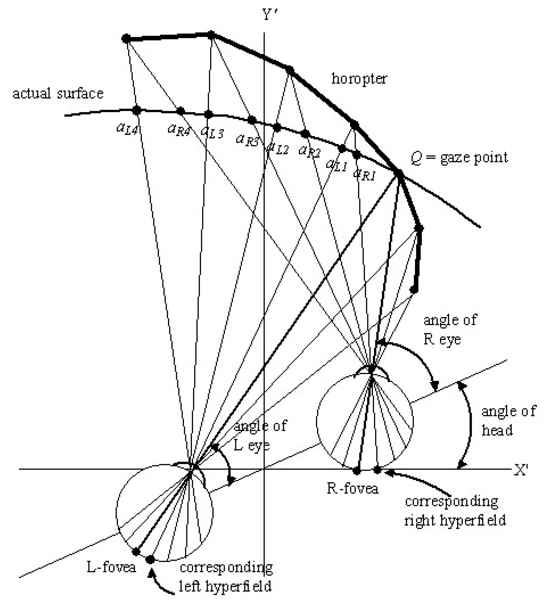
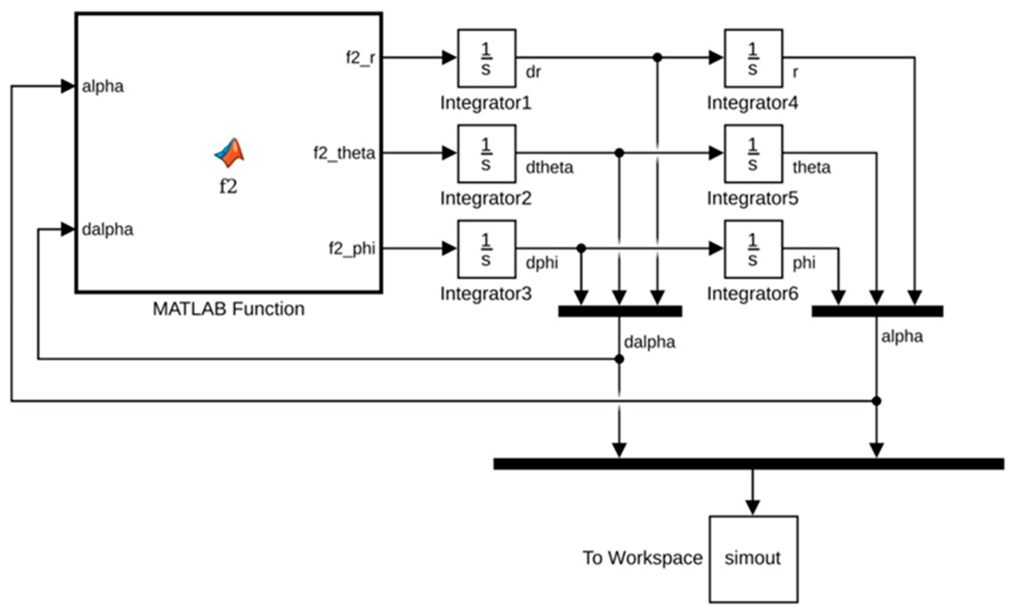
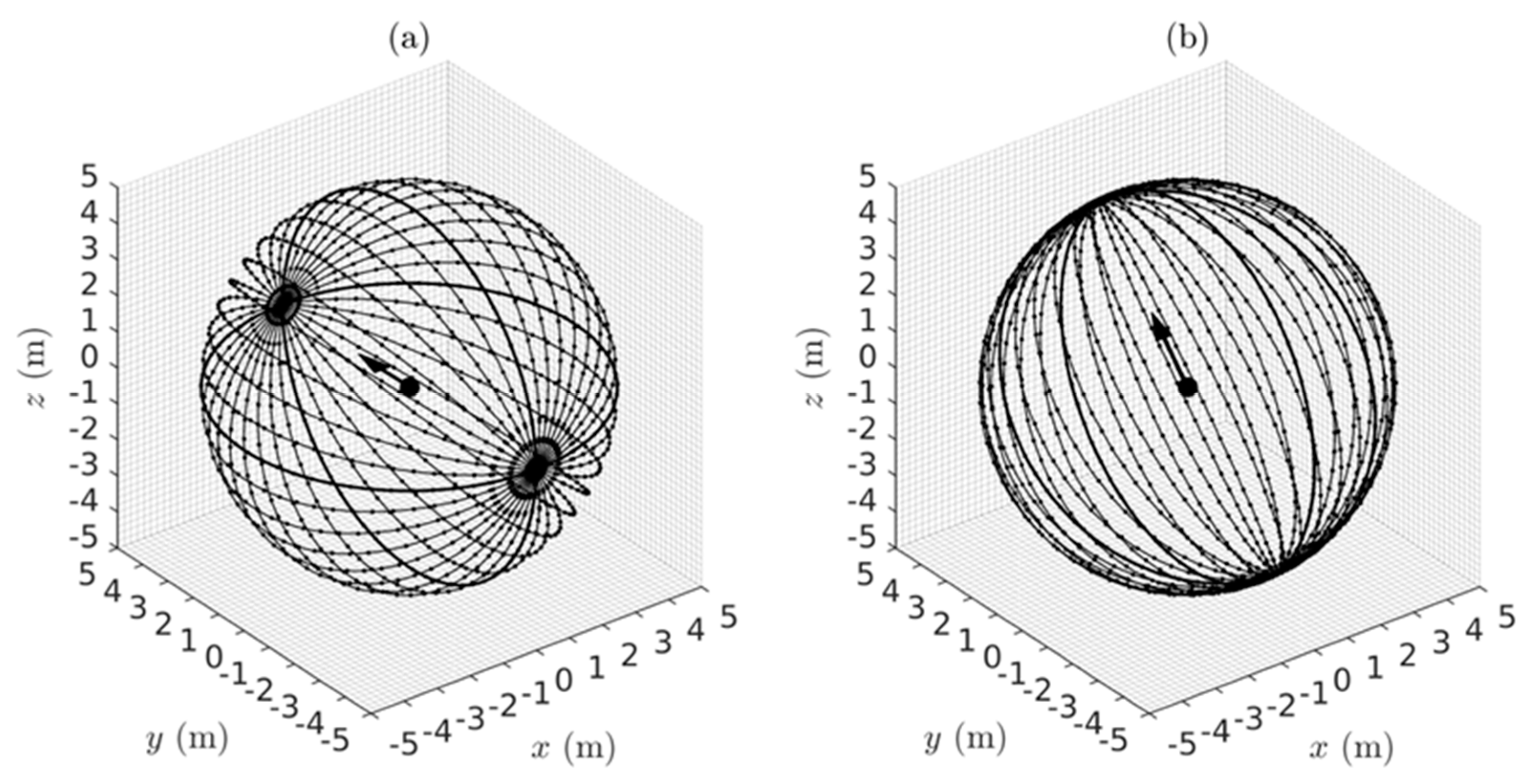
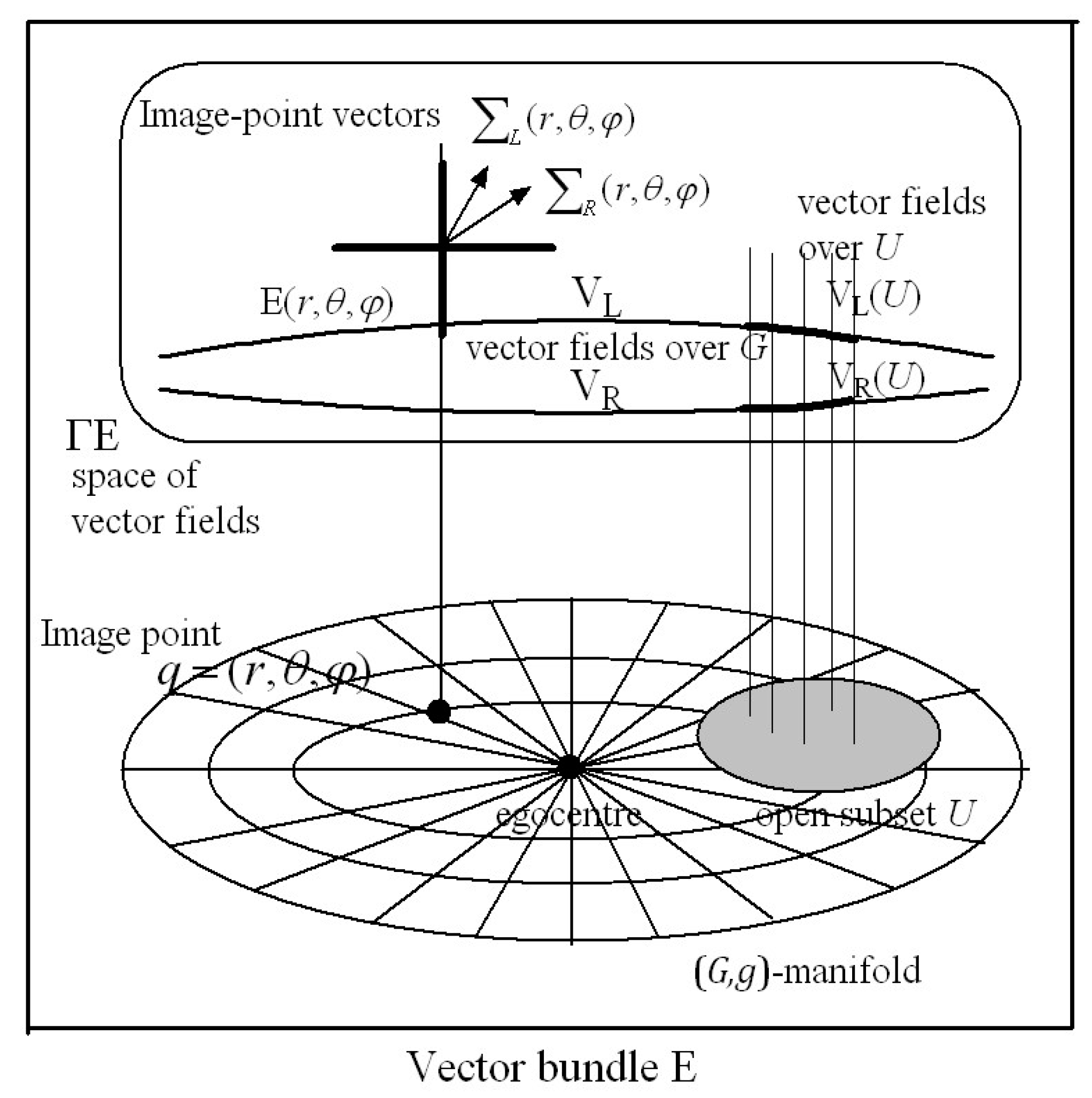


