Abstract
This work proposes a procedure for the multi-objective design of a robust forecasting ensemble of data-driven models. Starting with a data-selection algorithm, a multi-objective genetic algorithm is then executed, performing topology and feature selection, as well as parameter estimation. From the set of non-dominated or preferential models, a smaller sub-set is chosen to form the ensemble. Prediction intervals for the ensemble are obtained using the covariance method. This procedure is illustrated in the design of four different models, required for energy management systems. Excellent results were obtained by this methodology, superseding the existing alternatives. Further research will incorporate a robustness criterion in MOGA, and will incorporate the prediction intervals in predictive control techniques.
1. Introduction
Forecasting is important in every field of science, as it enables taking informed decisions in the future. In energy systems, energy forecasting plays an essential role in energy sector development, policy formulation, and management of these systems [1]. Throughout the years, different models have been developed and applied for forecasting. As data-driven models, due to their universal approximation property, have consistently increased their application in energy systems, they will be focus of this work.
Many techniques and forecasting methods have been published regarding energy systems. Wang and co-workers [2] discuss deterministic and probabilistic methods using deep learning for forecasting in renewable energy applications. A review on the use of multi-objective optimization for wind energy forecasting is presented in [3]. In [4], an evaluation of forecasting applications for energy storage systems is conducted. Forecasting algorithms and energy management strategies for microgrids are extensively presented in [5]. Energy consumption forecasting is discussed in [6], focusing on the manufacturing industry. Concerning Home Energy Management Systems (HEMS), to obtain energy or economic savings it is mandatory to accurately forecast the energy consumption, or the load demand, and the energy or power produced by the renewable sources [7,8].
Ensemble learning is a strategy which involves deriving a high-level prediction model by combining the predictions of multiple models in order to obtain better forecasting accuracy than the one obtained from any of the individual models. Three basic approaches to ensemble modelling are bagging, boosting, and stacking.
A bagged ensemble model creates a high-level model by averaging the predictions of a set of typically homogenous models trained on different random splits of the training data [9]. In contrast, boosted ensemble modelling involves improving models sequentially using the residuals from the current model to target the training of subsequent models [10]. On the other hand, stacking ensembles typically involves combining the predictions of strong, diverse models in an overall high-level model.
In the field of energy management systems, the use of ensembles of models are discussed in [11] for solar radiation prediction, in [12] for PV power forecasting, and in [13] for load forecasting, just to name a few references.
Ensembles of deterministic forecasting models are common solutions in energy management systems. However, such forecasts convey little information about the possible future state of a system, and since a forecast is inherently erroneous, it is important to quantify the correspondent error. We enter here a discussion on the field of probabilistic forecasting, whose goal is to provide either a complete predictive density of the future state or to predict that the future state of a system will fall within an interval defined by a confidence level. We shall denote here these models as robust models. Different techniques have appeared in the literature to determine these prediction intervals for data-driven models. To the best of our knowledge, the earliest publication on the subject is [14], closely followed by the work of Hang and co-workers [15]. Afterwards, several approaches have been proposed, the majority of them being summarized in the excellent review of Cartagena et al. [16].
In the area of energy systems, most of the work has been focused on probabilistic load forecasting. The works of Khosravi and colleagues [17], Quan et al. [18], Gob and co-workers [19], Antoniadis et al. [20], and Zuniga-Garcia and co-workers [21] are important contributions in this area. Publications on solar radiation forecasting with prediction intervals include [22,23]. Excellent reviews in probabilistic forecasting of photovoltaic power production and electricity price forecasting can be found in [24,25], respectively.
The area of ensemble probabilistic forecasting is narrower, but currently very active. Worthwhile works on this topic can be read in [2,26,27]
To the best of our knowledge, we cannot find in the literature a multi-objective design of ensemble forecasting models that simultaneously provides prediction intervals. For this reason, a simple and efficient procedure for model design is proposed, incorporating data selection, feature selection, parameter estimation, model ensemble selection, and prediction intervals determination, which constitutes the major contribution of this paper.
To be able to propose a simple approach, the detailed research questions to be addressed are:
- -
- Is the performance of ensemble forecasting models better than single ones?
- -
- In previous works [28], 25 models were used for the ensemble. Would a larger number result in better performance?
- -
- For NARX models (using exogeneous variables), which would be the best technique for describing the evolution of exogenous variables?
- -
- Is the Prediction Interval Coverage Probability threshold meet for all steps within the Prediction Horizon?
The paper is organized as follows: Section 2 introduces the background on single-model design using a multi-objective formulation, the model ensemble, the calculation of prediction intervals and the performance criteria to be used throughout this work. Section 3 describes the data that will be used, the design of four different models: solar radiation, atmospheric air temperature, load demand, and PV power generation models, analyzing and discussing the results obtained. A model design procedure is also detailed here. General conclusions and further research lines are given in Section 4.
2. Materials and Methods
This section will first describe the procedure used for single model design, starting from data selection. For the class of data-driven models whose parameters are separate, such as radial basis function networks employed in this paper, training algorithms are discussed. Feature and topology selection are performed using a multi-objective algorithm (MOGA). Model ensembles, using the MOGA results, are discussed afterwards. Methods to determine prediction intervals are then discussed. This section ends with the performance criteria to be used in the next section.
2.1. Single Model Design
To obtain “good” models from a set of acquired or existent data, three sub-problems must be solved:
- A pre-processing stage where, from the existing data, suitable sets (training, testing, validation, etc.) are obtained; this is known as a data selection problem;
- Determination of the “best” set of inputs (feature/delays selection) and network topology, given the above data sets;
- Determination of the “best” network parameters, given the data sets, inputs/delays and network topology.
These sub-problems are solved by the application of a model design framework, composed of two existing tools. The first, denoted as ApproxHull, performs data selection, from the data available for design. The feature and topology search are solved by the evolutionary part of MOGA (Multi-Objective Genetic Algorithm), while parameter estimation is performed by the gradient part of MOGA.
2.1.1. Data Selection
To design data driven models like RBFs (Radial Basis Functions), it is mandatory that the training set involves the samples that enclose the whole input–output range where the underlying process is supposed to operate. To determine such samples, called convex hull (CH) points, out of the whole dataset, convex hull algorithms can be applied.
The standard convex hull algorithms suffer from both exaggerated time and space complexity for high-dimension studies. To tackle these challenges in high dimensions, ApproxHull was proposed in [29] as a randomized approximation convex hull algorithm. To identify the convex hull points, ApproxHull employs two main computational geometry concepts: the hyperplane distance and the convex hull distance.
Given the point in a d-dimensional Euclidean space, and a hyperplane H, the hyperplane distance of x to H is obtained by:
where and d are the normal vector and the offset of H, respectively.
Given a set and a point , the Euclidean distance between x and the convex hull of X, denoted by conv(X), can be computed by solving the following quadratic optimization problem:
where , , and . Assuming that the optimal solution of Equation (2) is a*, the distance of point x to conv(X) is given by:
ApproxHull consists of five main steps. In Step 1, each dimension of the input dataset is scaled to the range [−1, 1]. In Step 2, the maximum and minimum samples with respect to each dimension are identified and considered as the vertices of the initial convex hull. In Step 3, a population of k facets based on the current vertices of the convex hull is generated. In Step 4, the furthest points to each facet in the current population are identified using Equation (1), and they are considered as the new vertices of the convex hull, if they have not been detected before. Finally, in Step 5, the current convex hull is updated by adding the newly found vertices into the current set of vertices. Step 3 to Step 5 are executed iteratively until no vertex is found in Step 4 or the newly found vertices are very close to the current convex hull, thus containing no useful information. The closest points to the current convex hull are identified using the convex hull distance shown in (3) under an acceptable user-defined threshold.
In a prior step before determining the CH points, ApproHull eliminates replicas and linear combinations of samples/features. After having identified the CH points, ApproxHull generates the training, test and validation sets to be used by MOGA, according to user specifications, but incorporating the CH points in the training set.
2.1.2. Parameter Separability
We shall be using models that are linear–nonlinearly separable in their parameters [30,31]. The output of this type of model, at time step k, is given as:
In (4), is the ANN input at step k, is the basis functions vector, u is the (linear) output weights vector, and v represents the nonlinear parameters. For simplicity, we shall assume here only one hidden layer, and v is composed of n vectors of parameters, each one for each neuron . This type of model comprises Multilayer Perceptrons, Radial Basis Function (RBF) networks, B-Spline and Asmod models, Wavelet networks, and Mamdani, Takagi, and Takagi-Sugeno fuzzy models (satisfying certain assumptions) [32].
This means that the model parameters can be divided into linear and nonlinear parameters:
and that this separability can be exploited in the training algorithms. For a set of input patterns X, training the model means finding the values of w, such that the following criterion is minimized:
where denotes the Euclidean norm. Replacing (4) in (6) we have:
where , m being the number of patterns in the training set. As (7) is a linear problem in u, its optimal solution is given as:
Where the symbol ‘+’ denotes a pseudo-inverse operation. Replacing (8) in (7), we have a new criterion, which is only dependent on the nonlinear parameters:
The advantages of using (9) instead of (7) are threefold:
- It lowers the problem dimensionality, as the number of model parameters to determine is reduced;
- The initial value of is much smaller than
- Typically, the rate of convergence of gradient algorithms using (9) is faster than using Equation (7).
2.1.3. Training Algorithms
Any gradient algorithm can be used to minimize (7) or (9). First-order algorithms, error back-propagation (or steepest descent method), conjugate gradient method or their variants, or second-order methods, such as quasi-Newton, Gauss–Newton or Levenberg–Marquardt (LM) algorithms can be employed. For non-linear least-squares problems, the LM method [33,34] is recognized to be the state-of-the-art method, as it exploits the sum-of-squares characteristics of the problem. The LM search direction is given as the solution of:
where is the gradient vector:
Additionally, is the Jacobean matrix:
is a regularization parameter, which enables the search direction to change between the steepest descent and the Gauss–Newton directions.
It has been proved in [35] that the gradient and Jacobean of criterion (9) can be obtained by: (a) first computing (8); (b) replacing the optimal values in the linear parameters; (c) and determining the gradient and Jacobian in the usual way.
Typically, the training algorithm terminates after a predefined number of iterations, or using an early stopping technique [36].
2.1.4. Radial Basis Function Networks
In the case described here, RBF models will be employed. The basis functions employed by RBFs are typically Gaussian functions:
which means that the nonlinear parameters for each neuron are constituted by a center vector, , with as many components as the dimensions of the input, and a spread parameter, . The derivatives of the basis function with respect to the nonlinear parameters are:
Associated with each model, there are always heuristics that can be used to obtain the initial values of the parameters. For RBBs, center values can be obtained randomly from the input data, or from the range of the input data. Alternatively, clustering algorithms can be employed. Initial spreads can be chosen randomly, or by using several heuristics, such as:
where zmax represents the maximum distance between centers.
2.1.5. MOGA
This framework is described in detail in [37], and it will be briefly discussed here. MOGA evolves ANN structures, whose parameters separate (in this case RBFs), with each structure being trained by minimizing criterion (9) in Section 2.1.3. As we shall be designing forecasting models, where we want to predict the evolution of a specific variable within a predefined PH (Prediction Horizon), the models should provide multi-step-ahead forecasting. This type of forecast can be achieved in a direct mode, by having several one-step-ahead forecasting models, each providing the prediction of each-step-ahead within a PH. An alternative method, which is followed in this work, is to use a recursive version. In this case, only one model is used, but its inputs evolve with time. Consider the Nonlinear Auto-Regressive model with Exogeneous inputs (NARX), with just one input, for simplicity:
where denotes the prediction for time-step k + 1 given the measured data at time k, and the jth delay for variable i. This represents the one-step-ahead prediction within a prediction horizon. As we iterate (17) over PH, some or all of the indices in the right-hand-side will be larger than k, which means that the corresponding forecast must be employed. What has been said for NARX models is also valid for NAR models (with no exogeneous inputs).
The evolutionary part of MOGA evolves a population of ANN structures. Each topology comprises of the number of neurons in the single hidden layer (for a RBF model), and the model inputs or features. MOGA assumes that the number of neurons must be within a user-specified bound, Additionally, one needs to select the features to use for a specific model, i.e., must perform input selection. In MOGA we assume that, from a total number q of available features, denoted as F, each model must select the most representative d features within a user-specified interval, . For this reason, each ANN structure is codified as shown in Figure 1:
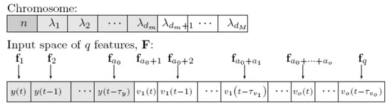
Figure 1.
Chromosome and input space lookup table [37].
The first component corresponds to the number of neurons. The next dm represent the minimum number of features, while the last white ones are a variable number of inputs, up to the predefined maximum number. The values correspond to the indices of the features fj in the columns of F.
The operation of MOGA is a typical evolutionary procedure. We shall refer the reader to publication [37] regarding the genetic operators.
The model design cycle is illustrated in Figure 2. First, the search space should be defined. That includes the input variables to be considered, the lags to be considered for each variable, and the admissible range of neurons and inputs. The total input data, denoted as F, together with the target data, must then be partitioned into three different sets: training set, to estimate the model parameters; test set, to perform early stopping; and validation set, to analyze the MOGA performance.
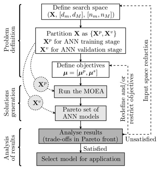
Figure 2.
Model design cycle [29].
Secondly, the optimization objectives and goals need to be defined. Typical objectives are Root-Mean-Square Errors (RMSE)-evaluated on the training set (), or on the test set (), as well as the model complexity, #(v)—number of nonlinear parameters—or the norm of the linear parameters (). For forecasting applications, as it is the case here, one criterion is also used to assess its performance. Assume a time-series sim, a subset of the design data, with p data points. For each point, the model (14) is used to make predictions up to PH steps ahead. Then, an error matrix is built:
where e[i,j] is the model forecasting error taken from instant i of sim, at step j within the prediction horizon. Denoting the RMS function operating over the ith column of matrix E, by , the forecasting performance criterion is the sum of the RMS of the columns of E:
Notice that every performance criterion can be minimized, or set as a restriction, in the MOGA formulation.
After having formulated the optimization problem, and after setting other hyperparameters, such as the number of elements in the population (npop), number of iterations population (niter), and genetic algorithm parameters (proportion of random immigrants, selective pressure, crossover rate and survival rate), the hybrid evolutive-gradient method is executed.
Each element in the population corresponds to a certain RBF structure. As the model is nonlinear, a gradient algorithm such as the LM algorithm minimizing (6) is only guaranteed to converge to a local minimum. For this reason, the RBF model is trained a user-specified number of times, starting with different initial values for the nonlinear parameters. MOGA allows initial centers chosen from the heuristics mentioned in Section 2.1.4, or using an adaptive clustering algorithm [38].
As the problem is multi-objective, there are several ways for identifying which training trial is the best one. One strategy is to select the training trial whose Euclidean distance from the origin is the smallest. The green arrow in Figure 3 illustrates this situation for . In the second strategy, the average of objective values for all training trails is calculated, and then the trial whose value is the closest to the average value will be selected as the best one (i.e., red arrow in Figure 3).
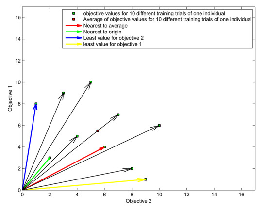
Figure 3.
Different strategies for identifying the best out of 10 training trials.
The other strategies are to select the training trial which minimized the objective (i.e., ) better than the other trials. As an example, the yellow and blue arrows in Figure 3 are the best training trials which minimized objective 1 and objective 2, respectively.
After having executed the specified number of iterations, we have performance values of npop * niter different models. As the problem is multi-objective, a subset of these models corresponds to non-dominated models (nd), or Pareto solutions. If one or more objectives is (are) set as restriction(s), a subset of nd, denoted as preferential solutions, pref, corresponds to the non-dominated solutions, which meet the goals. An example is shown in Figure 4.
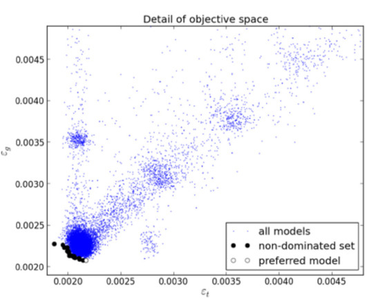
Figure 4.
Detail of objective space for a problem discussed in [39].
The performance of MOGA models is assessed on the non-dominated model set, or in the preferential model set. If a single solution is sought, it will be chosen on the basis of the objective values of those model sets, performance criteria applied to the validation set, and possibly other criteria.
When the analysis of the solutions provided by the MOGA requires the process to be repeated, the problem definition steps should be revised. In this case, two major actions can be carried out: input space redefinition by removing or adding one or more features (variables and lagged input terms in the case of modelling problems), and improving the trade-off surface coverage by changing objectives or redefining goals. This process may be advantageous, as usually the output of one run allows us to reduce the number of input terms (and possibly variables for modelling problems) by eliminating those not present in the resulting population. Additionally, it usually becomes possible to narrow the range for the number of neurons in face of the results obtained in one run. This results in a smaller search space in a subsequent run of the MOGA, possibly achieving a faster convergence and better approximation of the Pareto front.
Typically, for a specific problem, an initial MOGA execution is performed, minimizing all objectives. Then, a second execution is run, where typically some objectives are set as restrictions.
2.2. Model Ensemble
As has been pointed out, the output of MOGA is not a single model, but sets of nondominated RBFs and, possibly, preferential models. These are typical powerful models, all with a different structure, that can be used to form a stacking ensemble.
Several combination approaches have been applied for forecasting models. The most usual way is the use of the mean, against which other alternatives are compared. The authors of [40] propose four approaches: the median, the use of weights proportional to the probability of success, the use of weights calculated by variance minimization, and the use of weights calculated from eigenvector of covariance matrix of forecast errors. Other alternatives are even more complex. For instance, in [41], a Bayesian combination approach for combining ANN and linear regression predictor was used. In [42], a combination of weather forecasts from different sources using aggregated forecast from exponential reweighting is proposed.
The models discussed here are intended to be used in model predictive control applications where, in one step, hundreds or thousands of these models must be executed, each one PH times. This way, a computationally simple technique of combining the outputs of the model ensemble must be employed. As in a few exceptional cases, MOGA-generated models have been found with outputs that can be considered as outliers, the ensemble output is obtained as a median, and not as a mean. The ensemble output, using a set of models denoted as outset, is given as:
This was proposed in [28], where the number of models in the ensemble was discussed. Among the three possibilities (10, 25, and 50), it was found that the performance of 10 models could be improved if 25 models were chosen. On the other hand, the small improvement that was obtained by doubling the number of models did not justify the increase in computational complexity.
Having experimentally found a convenient number of models to use in the ensemble, the selection of those 25 models has not been deeply addressed, i.e., the selection of models to be included in outset; this will be addressed in this paper.
2.3. Robust Models
The recent inclusion of smart grids and renewable integration requirements has induced the drawback of increasing the uncertainty of future supply, demand, and prices. Academics and practitioners alike have realized that probabilistic electricity price, load, and production forecasting is now more important for energy systems planning and operations than ever before [24,25].
Predictive modeling assumes that all observations are generated by a data generating function f(x) combined with additive noise:
where is the point forecast of the variable at time k made at an earlier point in time and is a data nose term, responsible for introducing uncertainty in the model. This can be decomposed into three terms: one related to model misspecification, related to the fact that the model, with its optimal parameters and data conditions, can only approximate the real underlying function generating the data; training data uncertainty, related to the uncertainty over how representative the training data is with respect to the whole operational range of the model input; and parameter uncertainty, related to the fact that the parameters might not be the optimal ones.
The most common extension from point to probabilistic forecasts is to construct prediction intervals (PIs). A number of methods can be used for this purpose; the most popular takes into account both the point forecast and the corresponding error: the center of the PI at the (1 − α) confidence level is set equal to and its bounds are α/2th and (1 − α/2)th quantiles of the cumulative distribution function of . For instance, for the commonly used 90% PIs, which is the level used in this paper, the 5% and 95% quantiles of the error term are required. We will denote as and the upper and lower bounds, respectively.
A basic method to find these bounds relies on the use of the PDF (Probability Density Function) of y, assumed known. However, in practice, a PDF cannot be estimated perfectly, and therefore there will be error propagation when computing the interval. For this reason, if one is only interested in the PI and does not need all the information in the PDF, it is more convenient to use a method that estimates the PI without needing a known PDF.
When considering ANN models, the available methods for computing PIs can be categorized into two classes [16]:
- Sequential methods, which first receive the point forecast, and then use it to construct the PI;
- Direct methods, where the construction of the PI is carried out simultaneously with the identification. These are outside the scope of this paper. The reader is referred to [16] for a description of this class of methods.
In the first class, the sequential methods, five techniques can be pointed out:
- 1.
- Delta Method [15]
This method assumes that the noise variance is homogeneous and normally distributed. The total prediction variance for each prediction can be obtained as:
where is defined in (5), J in (12), and data noise variance, , can be estimated as:
where N denotes the total number of samples and p the number of model parameters. The bounds are assumed to be symmetric and given as:
where represents the α/2 quantile of a Student’s t-distribution with N − p degrees of freedom.
- 2.
- Bayesian Method
This method involves training the ANN as a Bayesian estimator (the ANN parameters are modelled as a probability distribution instead of single values). A posterior distribution for the network parameters given the training data points is estimated by applying Bayes’ Theorem, after which a Markov Chain Monte Carlo algorithm can be used to estimate the real posterior via a sampling procedure [14].
- 3.
- Mean-Variance Estimation Method (MVEM) [43]
The MVEM proposes that a PI can be built if two NNs are trained sequentially: the first for estimating point predictions, trained with a mean square error loss like any standard neural model, and the second for estimating prediction error variance, trained to estimate the error variance between each prediction and target data pairs.
- 4.
- Bootstrap method
This method assumes boosted ensemble modelling, and will not de described here.
- 5.
- Covariance method
This method is similar to the Delta method described above. In this case, and using the notation introduced before to denote the output of the last nonlinear layer, dependent on the input matrix, X, and the nonlinear parameters v, the total prediction variance for each prediction can be obtained as
where is the input training matrix.
In particular, we can use in (25) the optimal parameter values obtained after training, and . Notice that, due to the training of the model in MOGA, we have available (or can indirectly be obtained) , as well as , if belongs either to the test or validations sets. In other words, it is computationally cheap to compute (25) and, for this reason, is the method followed here.
2.4. Performance Criteria
To assess the quality of the models, both in terms of robustness and in terms of the quality of approximation, different criteria will be used.
Related to robustness, the interval width and the coverage level are two important metrics. These will be assessed by two criteria, the Prediction Interval Normalized Averaged Width (PINAW), and the Prediction Interval Coverage Probability (PICP), defined as:
where N is the number of samples considered, and are the upper and lower bounds, introduced in (24) of the model output for time k + 1, given the data available until time k, respectively, and R is the range of the system output in the whole training set:
PICP indicates if the interval given by the bounds contains the real measure of :
where
As we would like to assess the robustness of the estimation not only for the next time-ahead, but along PH, both PINAW and PICP must be determined for all steps within PH.
To assess the performance through the whole prediction horizon, the sum of (31) will be employed:
Additionally, PICP(s) will be assessed to determine violations of the level L specified (in this paper, L = 90%):
Several criteria can be used to assess the quality of the approximation. In this paper, the following will be employed: Root-Mean-Square of the Errors (RMSE) (36), Mean-Absolute Error (MAE) (37), Mean-Relative Error (MRE) (38), Mean-Absolute Percentage Error (MAPE) (39), and Coefficient of Determination, or R-Square (R2) (40). Please notice that these criteria are computed with data normalized in the interval [−1, 1].
Having defined the criteria that will be used to assess the performance of the different models, for each problem and to ease understanding, a notation describing the models must be introduced. First, we shall be comparing ensemble models with single models, chosen by the user. The former will be denoted by me, and the later by ms. Different sets will be used to determine the ensemble solutions, namely, using models from the set of non-dominated solutions obtained in the 1st MOGA execution, denoted as from the set of preferred set achieved in the 2nd MOGA execution (), as well as three sets of models selected from the preferred set; those will be denoted as , , and .
The set denoted as is defined as:
where
In (41), is the set of non-dominated models obtained in the 1st MOGA execution, is the set of the linear weight norm for each model in , and is its median.
In the same way, is the median of the sum of the forecasts for the prediction time-series obtained for all models in the set of non-dominated models obtained in the 1st MOGA execution.
Then is the set result of the intersection of the set of models whose weight norm is less than and the set of models whose forecast is less than .
Similarly, the set is defined as:
where is the set of preferred models obtained in the 2nd MOGA execution, is the median of the linear weight norm for each model in , and the median of the sum of the forecasts for the prediction time-series obtained by models .
The remaining three sets are subsets of , and are defined below.
i.e., is the subset of models whose linear weights belongs to the NS smallest weight norms.
Therefore, stands for the subset of models, from the preferred set, whose sum of the forecast errors in the prediction set belongs to the NS smallest forecasts. In this work, NS=25, as it has been found previously [28] that nothing was gained by increasing this number.
The third subset of models, , is obtained iteratively, by adding non-dominated models, considering nw(.) and fore(.) as the two criteria, until NS models are found. Initially, the set of models to be inspected, , is initialized to , and to an empty set. In each iteration, both criteria are applied to . Then, the non-dominated solutions found are added to and removed from .
For NAR models, these are the five sets of models to consider for the ensemble. For NARX models, however, we must consider how the forecasts of the exogeneous variables will be obtained. Three methods are obvious and will be used here. In the first case, measured values (m) will be used for the forecasts. This is the method against which the other two will be compared, as there will be no errors in the forecasts of the exogenous variables. The second technique will use the forecasts obtained using the single model (s) previously selected by the user. The third case will use the ensemble solution (e) that achieves the best results, for the corresponding exogeneous variable. Using as example , three different NARX models will be considered: , , and , corresponding to the three cases mentioned above.
3. Results and Discussion
3.1. The Data
To be able to determine a procedure that, given the output of a MOGA procedure, selects the models to be used in the ensemble, data acquired from a detached household situated in Montenegro, Algarve, Portugal, from the 1 July 2021 to the 31 July 2023, were employed. The house and the data acquisition system is described in [44], and the reader is encouraged to consult this reference. The data used here can be freely downloaded at https://zenodo.org/record/8096648 (accessed on 20 May 2023).
Weather data, atmospheric air temperature (T), and global solar radiation (R) were acquired at 1 min intervals. Power Demand (PD) was acquired with 1 sec intervals. PV Power generated (PG) was acquired with a sampling time of 1 min. All these data were averaged across 15 min intervals. Additional data that were used include the daily household occupation (Occ) and a codification for the type of day (DE). This characterizes each day of the week and the occurrence and severity of holidays based on the day they occur, as may be consulted in [45,46]. In Table 1, the regular day column shows the coding for the days of the week when these are not a holiday. The following column presents the values encoded when there is a holiday, and finally, the special column shows the values that substitute the regular day value in two special cases: for Mondays when Tuesday is a holiday and for Fridays when Thursday is a holiday.

Table 1.
Day encoding.
To be able to implement a predictive control strategy for Home Energy Management Systems, there is the need to forecast the PV power generated and the load demand. The latter can be modelled as a NARX model:
The use of the overline symbol in the last equation denotes a set of delayed values of the corresponding variable. The power generated can also be modelled as a NARX model:
The use of these exogeneous variables was discussed and justified in previous publications of the authors (please see [44,47,48]). In particular, these models use as exogeneous variables air temperature and solar radiation, which means that we need also to predict the evolution of these variables. The solar radiation can be modelled as a NAR model:
while the air temperature is modelled as:
Previously [28] these four models were designed with data ranging from 1 May 2020 00:07:30 to 31 August 2021 23:52:30 (nearly 16 months). The period used for forecasting during MOGA design is from 7 July 2020 13:07:30 to 27 July 2020 03:07:30 (1881 samples); for validation, the period between 4 July 2021 05:37:30 and 24 July 2021 03:22:30 was used, and 1962 samples were employed.
These models were employed for a completely different period, starting from 23-June-2022 23:07:30 to 01-August-2022 08:52:30 (1 year after). The evolution of the data, for this period, is illustrated in Figure 5, Figure 6 and Figure 7.
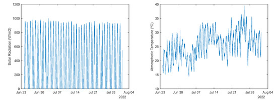
Figure 5.
Left: Solar radiation. Right: Atmospheric temperature.
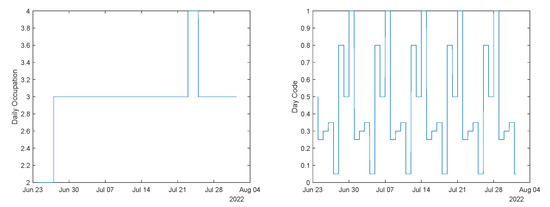
Figure 6.
Left: Daily occupation. Right: Day code.
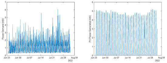
Figure 7.
Left: Power demand. Right: Power generated.
The design of the four different models is detailed in [28]. It will be briefly summarized here. For each model, two executions of MOGA were performed, with the first only minimizing four objectives, , , #(v) and , while in the second execution, some objectives were set as goals.
For all problems, MOGA was parameterized with the following values:
- Prediction horizon: 28 steps (7 h);
- Number of neuros: ;
- Initial parameter values: OAKM [38];
- Number of training trials: five, best compromise solution;
- Termination criterion: early stopping, with a maximum number of iterations of 50;
- Number of generations: 100;
- Population size: 100;
- Proportion of random emigrants: 0.10;
- Crossover rate: 0.70.
For models M3 and M4, the number of admissible inputs ranged from 1 to 30, while for M1 and M2 the range employed was from 1 to 20.
Typically, the power demand at any instant within a day is correlated to corresponding values one day before and, to a lesser extent, values observed one week before. For this reason, lags of the modelled and the exogenous variables were collected from three periods: immediately before the sample, centered at the corresponding instant one day before, and centered at the corresponding instant one week before. For this particular model, we used [20 9 9] for PD, [20 9 0] for T, [1 0 0] for Occ, and [1 0 0] for DE. This means that for PD we considered the first 20 lags before the current samples: nine centered 24 h ago and nine centered one week before. For T, the same number of lags before the current sample and centered one day ago will be used (but not from the third period), and for the other two variables only the first lag will be allowed. This means that the total number of lags (dmax) that MOGA considers is (20 + 9 + 9) + (20 + 9) + (1) + (1), i.e., 69 lags.
As data averaged in 15 min intervals are used, one week of data consists of 4 × 24 × 7 = 672 samples. With the additional four lags before one week of data, we have the largest delay index, lind = 676 samples. As a PH of 28 steps ahead was used, for this model, we obtain the following: npred_MOGA = 1881 − 676 − 28 = 1161 samples and npred_VAL = 1962 − 676 − 28 = 1242 samples.
For model 1, the solar radiation model, [20 9 9] lags were used, which means that dmax = 38, and lind, npred_MOGA, and npred_VAL are the same as M3.
Model 2, the air temperature model, used [20 9 0] lags, and the following values were obtained: dmax = 29, lind = 100, npred_MOGA = 1745 (around 18 days), and npred_VAL = 1826 (around 19 days).
Finally, model 4, the power generation model, uses [20 9 9] lags for PG, [20 9 9] lags for R, and [20 9 0] lags for T, which means that dmax = 105, and lind, npred_MOGA, and npred_VAL are the same as M1 and M3.
Before entering into the description of the results obtained with the single model and the different model ensembles, it should be noted that we shall use models designed for a PH of 28 steps ahead (7 h) and for a PH of 36 steps ahead (9 h).
3.2. Solar Radiation Models
The single model chosen was:
Some statistics related to the usage of the 341 non-dominated models are given in Table 2.
Table 2.
Non-dominated solutions statistics.
As can be seen, the RMSE values for the training set are higher than for the other sets. This is due to incorporation of the CH points in the training set. The RMSE values for the validation set are similar to the ones in the testing set, which demonstrates a good generalization of the models. The maximum values for the two columns are not shown because they are greater than 1017.
Table 3 shows the same statistics for the 204 preferred solutions.
Table 3.
Preferred solutions statistics.
Comparing Table 3 with Table 2, it can be concluded that a smaller dispersion for the RMSEs is obtained for the preferred solution.
Figure 8 show the 25 models selected from the set , for the sets , , and .
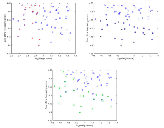
Figure 8.
Selected solar radiation models for (top left), (top right), and (bottom). In the top graphs, the selected models are denoted with a red cross, while for the bottom they are represented in green.
Obviously, there are common models between the three sets. In fact, , , and .
Table 4 illustrates the robustness and forecasting performance criteria, for the different sets of models. In this case, as the set of nondominated models is the same as the preferred (, the results are the same and will not be shown. Please note that, for each ensemble set described before, the median values for the corresponding models are shown in the line immediately below. They are denoted by the subscript mm. For each criterion associated with ensemble models, a Wilcoxon signed rank test is performed, with a level of significance of 0.05, to assess if the ensemble performance is statistically superior to the multiple models set. The inclusion of the symbol √ indicates if the test was successful.
Table 4.
Solar radiation performance values.
If we compare the performance of the single model against , the ensemble approach is better in all criteria. Overall, obtains the highest number of best results (marked in bold). For all criteria, except and , the ensemble approaches are statistically better than the corresponding multiple models.
Figure 9, Figure 10, Figure 11, Figure 12, Figure 13, Figure 14 and Figure 15 illustrate the evolution of , , RMSE(s), MAE(s), MRE(s), MAPE(s), and R2(s), over the prediction horizon, considering the set . On the left side of each figure, the selected ensemble is shown, and on the right, the evolution for the multiple models is presented. Figure 16 shows, for three days within the time-series considered, the measured solar radiation, its one-step-ahead forecast, and the corresponding upper and lower bounds.
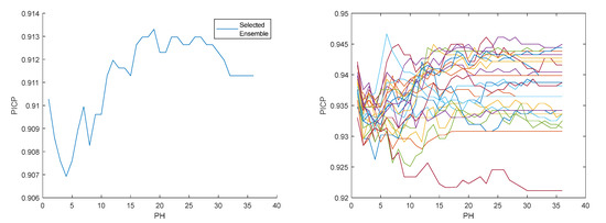
Figure 9.
Solar radiation PICP evolution. Left: Ensemble; Right: Multiple models.
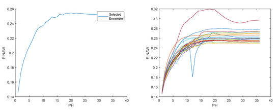
Figure 10.
Solar radiation PINAW evolution. Left: Ensemble; Right: Multiple models.
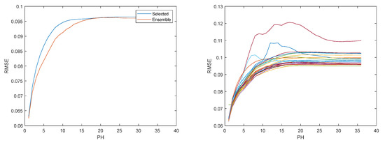
Figure 11.
Solar radiation RMSE evolution. Left: Ensemble; Right: Multiple models.
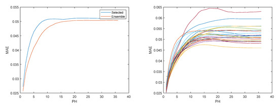
Figure 12.
Solar radiation MAE evolution. Left: Ensemble; Right: Multiple models.
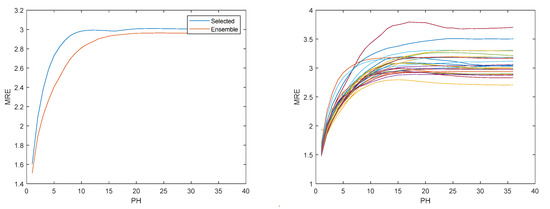
Figure 13.
Solar radiation MRE evolution. Left: Ensemble; Right: Multiple models.
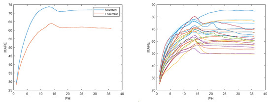
Figure 14.
Solar radiation MAPE evolution. Left: Ensemble; Right: Multiple models.
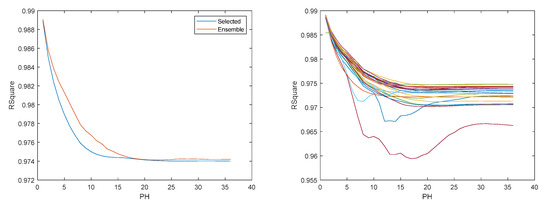
Figure 15.
Solar radiation R2 evolution. Left: Ensemble; Right: Multiple models.
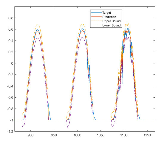
Figure 16.
Solar radiation one-step-ahead detail. Target (blue solid); Prediction (red solid); Prediction upper bound (yellow dash); Prediction lower bound (magenta dash).
As expected, the errors increase with the number of steps ahead considered. However, as it can be ascertained from the previous figures, it stays bounded.
3.3. Atmospheric Air Temperature Models
The single model chosen uses the following delays:
The model employs 90 neurons. Some statistics related to the usage of the 341 non-dominated models are given in Table 5.
Table 5.
Non-dominated solutions statistics.
As with solar radiation, the RMSE values for the validation set are similar to the ones in the testing set, which demonstrates a good generalization of the models. The maximum value of the weight norm is not shown because it is a very large number.
Table 6 shows the same statistics for the 204 preferred solutions.
Table 6.
Preferred solutions statistics.
The values are very close to the ones obtained for the non-dominated solutions.
Regarding the sets , , and , obtained from the set , the number of common models are , , and .
Table 7 illustrates the robustness and forecasting performance criteria, for the different sets of models. As with solar radiation, the set of selected models for the non-dominated and preferred solutions is the same, and the results will be shown only for the non-dominated case.
Table 7.
Air temperature performance values.
If we compare the performance of the single model against and , the ensemble approaches are better. Overall, obtains the best results, closely followed by . For all criteria, except and , the ensemble approaches are statistically better than the corresponding multiple models. Unlike the solar radiation models, air temperature models violate the PICP restriction for some steps within PH.
Figure 17, Figure 18 and Figure 19 illustrate the evolution of the performance criteria over PH, considering the set and, for three days within the time-series considered, the measured air temperature, its one-step-ahead forecast, and the corresponding upper and lower error bounds. For the sake of compactness, figures related to MAE and MRE evolution will not be shown.
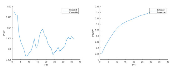
Figure 17.
Left: Air temperature PICP evolution. Right: Air temperature PINAW evolution.
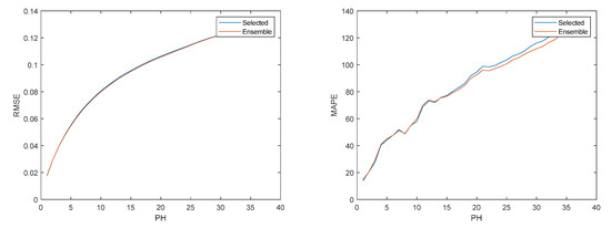
Figure 18.
Left: Air Temperature RMSE evolution. Right: Air Temperature MAPE evolution.
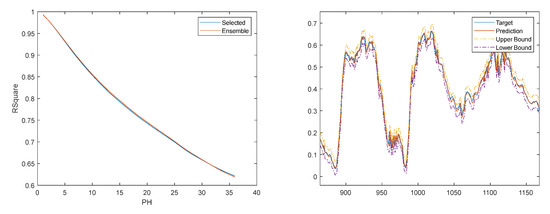
Figure 19.
Left: Air temperature R2 evolution. Right: Air temperature one-step-ahead detail. Target (blue solid); Prediction (red solid); Prediction upper bound (yellow dash); Prediction lower bound (magenta dash).
Comparing the evolution of the performance criteria with the corresponding figures for the air temperature model, we can observe that the errors do not stay bounded, but the rate of increase lowers with PH.
As can be seen, the majority of the measured samples lie within the bounds determined. The violations are found for periods where rapid changes happen.
3.4. Load Demand Models
The following single model with seven neurons is used:
Some statistics related to the usage of the 341 non-dominated models are given in Table 8.
Table 8.
Non-dominated solutions statistics.
As it can be seen, the maximum RMSE value for the validation set is very large. Sometimes, although not too often, MOGA-generated models have been found with the smallest value for one criterion, but with bad values for the others. Some values are not shown because they are very large.
Table 9 shows the statistics under analysis for the 179 preferred solutions.
Table 9.
Preferred solutions statistics.
Comparing Table 8 with Table 9, it can be concluded that a smaller dispersion for the RMSEs is obtained for the preferred solutions.
Analyzing Table 10, it is easy to conclude that the model ensemble always obtains the best results. Between the ensemble models obtained from the non-dominated set ( and the ones obtained from the preferential set (, the latter ones achieve better values. As expected, using measured values for the exogeneous variables ( produces better results than using forecasted values; in this latter case, the use of the ensemble solution ( always produces superior results than using the single model (. In the last table, the values in italics denote the best values, not using measured data.
Table 10.
Load demand performance values.
Having concluded that the best results were obtained using the set of models, this will be used for the subsequent phase. The number of common models is , , and . These models obtained the performance values shown in Table 11.
Table 11.
Load demand performance values.
Analyzing the last table, as expected, the best results were obtained by the set of models minimizing the weight norm. The difference is very large compared with the two other alternatives. Comparing the set of models using measured values as exogeneous variables with the forecast versions, for every criteria except and , the use of measured values obtains better values. This was also expected, as, in that case, there are no forecasting errors for the exogeneous variables. In every case, the use of the ensemble approach for the exogeneous variables obtained better results than the single model.
Overall, obtained better results than and , except for , and in particular, achieves the best compromise. Figure 20, Figure 21 and Figure 22 show the results obtained for this latter technique.
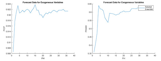
Figure 20.
Left: Load demand PICP evolution; Right: Load demand PINAW evolution.
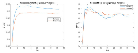
Figure 21.
Left: Load demand RMSE evolution; Right: Load demand MAPE evolution.
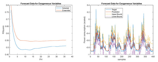
Figure 22.
Left: Load demand R2 evolution; Right: Load demand one-step-ahead detail. Target (blue solid); Prediction (red solid); Prediction upper-bound (yellow dash); Prediction lower bound (magenta dash).
3.5. Power Generation Models
The single model chosen was:
Some statistics related to the usage of the 295 non-dominated models are given in Table 12.
Table 12.
Non-dominated solutions statistics.
As observed, the maximum RMSE value for the validation set is very large. Some values are not shown because of their huge size.
Table 13 shows the same statistics for the 186 preferred solutions.
Table 13.
Preferred solutions statistics.
Comparing Table 13 with Table 12, it can be concluded that a smaller dispersion for the RMSEs is obtained for the preferred solutions. Still, the maximum value for RMSEval is very high.
As in the previous case, better solutions are obtained using the preferential set. For this reason, the values for the non-dominated set will not be shown.
Analyzing the results shown in Table 14, all ensemble models violated the PICP criterion, for all steps. In terms of the measured data for the exogeneous variables, the single model obtained a better performance than the ensemble for three out of the six criteria. Comparing the two methods of forecasting for the exogeneous variables, the ensemble approach obtained always the best results, except for the ensemble . obtained the best results using forecasted values for the exogeneous variables.
Table 14.
Power generation performance values.
As a consequence, we shall use the set of models for the subsequent phase. The number of common models between the three selection approaches is , , and . These models obtained the performance values shown in Table 15.
Table 15.
Power consumption performance values.
Analyzing the results presented in the last table, unexpectedly, the best results were obtained by the set of models in the Pareto front. The worst results were obtained by the set of models minimizing the weight norm.
The set of models using measured values as exogeneous variables with the forecast versions obtains the best results, with a difference slightly larger than for the power consumption. This might be because there are two exogenous dynamic variables, rather than only one. Regarding the set of models that use forecasting values, and obtained three first places each.
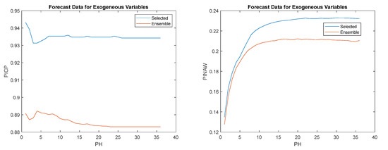
Figure 23.
Left: Power generation PICP evolution; Right: Power generation PINAW evolution.
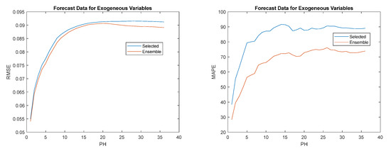
Figure 24.
Left: Power generation RMSE evolution; Right: Power generation MAPE evolution.
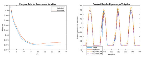
Figure 25.
Left: Power generation R2 evolution; Right: Power generation one-step-ahead detail. Target (blue solid); Prediction (red solid); Prediction upper-bound (yellow dash); Prediction lower bound (magenta dash).
3.6. Analysis of the Results
Analyzing the results presented, and taking into consideration the research questions formulated in the Introduction, we can conclude that the following:
- -
- In three out of four models, the ensemble versions present better results, for all performance criteria, than the single model chosen. In the power generation model, in three of the performance indices, the single model obtained the best results. Overall, for the total number of 24 criteria, the ensemble approaches obtained the best results in 21 cases;
- -
- Focusing now on the number of models to use in the ensemble, only in two performance criteria ( in the air temperature model and in the power generation model with measured data for the exogeneous variables) out of the 24 criteria did the use of more than 25 models obtain better results;
- -
- Regarding the method to select the 25 models (, or ), there is not a clear choice. The winners obtained for the selection methods were 8, 6, and 9, respectively;
- -
- For the NARX models, for all cases, the use of was found to be the best choice;
- -
- Finally, violations of PIPC were assessed using (35). As it can be seen in Table 4, Table 7, Table 11 and Table 14, and in Figure 9, Figure 17, Figure 20 and Figure 23, in most cases the computed Prediction Interval Coverage Probability, throughout PH for the chosen model ensemble, was slightly larger than the level specified, 90%. In the cases where violations have been found, PICP values are near 90%.
We can therefore propose the following procedure for model design:
- 1.
- Use ApproxHull to select the datasets from the available design data;
- 2.
- Formulate MOGA, in a first step, minimizing the different objectives;
- 3.
- Analyze MOGA results, restrict some of the objectives and redefine input space and/or the model topology;
- 4.
- Use the preferential set of models obtained from the second MOGA execution;
- 5.
- Determine using (44);
- 6.
- From obtain using (47);
- 7.
- If the model that should be designed is a NARX model, use for the exogenous variables;
- 8.
- Obtain the prediction intervals using (24) and (25).
The ensemble outputs are given by (20).
3.7. Discussion
A comparison of results obtained with this procedure with other proposals found in the literature is not completely fair to the proposed technique. As reported earlier, the four models used in this work were designed with data from May 2020 to August 2021. Additionally, in their design, a PH of 28 steps was considered. The results assessed here use essentially the whole month of July 2022. A PH of 36 steps is employed here, this larger value being justified in [49].
The values of solar radiation and atmospheric air temperature will not have changed so much from 2020–2021 to 2022 and, as the PV installation is the same, the same can be hypothesized to the evolution of the power generated. The same cannot be said in relation of the load demand, as several electric equipment were changed during 2022. For this reason, comparisons will only be applied to the solar radiation and generated power. Only papers providing values of PICP and PINAW for their results, and with a time resolution and prediction horizon convenient will be considered.
Chu and Coimbra [23] aimed at predicting Direct Normal Irradiance (DNI) by utilizing k-Nearest Neighbors (KNN) models, with forecast horizon of 5–20 min at 1 min resolution. In this case, the number of neighbors was set to 30 and was weighted based on the distance between them and the observation. The authors used lagged DNI observations as endogenous inputs and lagged Diffuse Horizontal Irradiance and sky image features as exogenous inputs. The results showed that the k-NN ensemble outperformed both the persistence ensemble and k-NN with assumed Gaussian distribution. The authors reported, for a nominal confidence level of 90%, PICP between 0.91 and 0.93 and PINAW between 31% and 70% for a 15 min horizon. For the same horizon, RMSE values varied between 107 and 208 W/m2. Our approach obtained, for 15 min step-ahead, values of 0.91, 14.5%, and 35 W/m2, respectively.
Galván and co-workers [50] addressed the estimation of prediction intervals for the integration of four Global Horizontal Irradiance (GHI) forecasting models (Smart Persistence, WRF-solar, CIADcast, and Satellite). With data collected at Sevilla, Spain, the best results obtained for PINAW for 15, 30, 45, and 60 min forecasting were 28%, 29%, 30%, and 32%, respectively. Using Figure 10, our technique obtained values between 14.5% and 19%.
Ni and co-workers [51] proposed an extreme learning machine (ELM) technique, combined with bootstrap to forecast the PV-generated power, for a time-step of 5 min. Prediction intervals were obtained using the bootstrap technique. Using L = 90%, the PICP obtained ranged between 92% to 94%. PINAW values ranged between 12% and 13%, a value close to the one that was obtained here for a 15 min step-ahead. The same authors, to prevent the instability of the ELM machine learning method in generating reliable and informative PIs, proposed in [52] an ensemble approach based on ELM and the Lower Upper Bound Estimation (LUBE) approach. The results, for the same 5 min horizon, increased the PICP to a range of 95–99%, and PINAW ranging from 9% to 14%.
As a final note, although the examples in this paper are from the energy arena, the proposed procedure is beneficial for all forecasting applications. ApproxHull and/or MOGA have been applied, for instance, in hydrological applications [39], Ground Penetrating Radar (GPR) applications [53], medical imageology [54], and temperature estimation in human tissues [55], to name just a few. All these applications will profit from the approach introduced here.
4. Conclusions
We have introduced a simple and efficient procedure for designing robust forecasting ensemble models that satisfy a multi-objective optimization problem. The procedure has been validated experimentally using four different models that are used in energy-based problems. The results obtained with this procedure compare favorably with existing proposals found in the literature.
The proposed procedure can be further exploited in two different directions. As models are designed using a multi-objective approach, a robustness criterion, such as minimizing the Prediction Interval Normalized Averaged Width over the prediction horizon (32) can be added to the problem formulation. This will make MOGA a little bit slower, but not greatly as a decomposition of —the matrix of the outputs of the last hidden layer over the training set of the optimal models—makes the computation of (25) less complicated.
The other research direction is the incorporation of the computed prediction intervals in predictive control techniques. This is an active field of research in several application areas, and in particular in the area of energy. The key contribution here, in relation with to other approaches, is the forecasting quality of our models, which has been demonstrated in this paper.
5. Patents
This work is protected under the Portuguese Patent Pending NO. 118847: “Computer-Implemented Method for Community Energy Management Using Mixed-Integer Linear Programming, Model Predictive Control, Non-Invasive Load Monitoring Techniques, Robust Forecasting Models and Related System”.
Author Contributions
The authors contributed equally for this work. All authors have read and agreed to the published version of the manuscript.
Funding
The authors would like to acknowledge the support of Operational Program Portugal 2020 and Operational Program CRESC Algarve 2020, grant number 72581/2020. A. Ruano also acknowledges the support of Fundação para a Ciência e Tecnologia, grant UID/EMS/50022/2020, through IDMEC under LAETA. M.G. Ruano also acknowledges the support of Foundation for Science and Technology, I.P./MCTES through national funds (PIDDAC), within the scope of CISUC R&D Unit—UIDB/00326/2020 or project code UIDP/00326/2020.
Data Availability Statement
The data that was used for this work can be downloaded from https://zenodo.org/record/8096648 (accessed on 20 May 2023).
Conflicts of Interest
The authors declare no conflict of interest.
References
- Ahmad, T.; Chen, H. A review on machine learning forecasting growth trends and their real-time applications in different energy systems. Sustain. Cities Soc. 2020, 54, 102010. [Google Scholar] [CrossRef]
- Wang, H.; Lei, Z.; Zhang, X.; Zhou, B.; Peng, J. A review of deep learning for renewable energy forecasting. Energy Convers. Manag. 2019, 198, 111799. [Google Scholar] [CrossRef]
- Liu, H.; Li, Y.; Duan, Z.; Chen, C. A review on multi-objective optimization framework in wind energy forecasting techniques and applications. Energy Convers. Manag. 2020, 224, 113324. [Google Scholar] [CrossRef]
- Sharma, V.; Cortes, A.; Cali, U. Use of Forecasting in Energy Storage Applications: A Review. IEEE Access 2021, 9, 114690–114704. [Google Scholar] [CrossRef]
- Ma, J.; Ma, X. A review of forecasting algorithms and energy management strategies for microgrids. Syst. Sci. Control. Eng. 2018, 6, 237–248. [Google Scholar] [CrossRef]
- Walther, J.; Weigold, M. A Systematic Review on Predicting and Forecasting the Electrical Energy Consumption in the Manufacturing Industry. Energies 2021, 14, 968. [Google Scholar] [CrossRef]
- Gomes, I.; Bot, K.; Ruano, M.d.G.; Ruano, A. Recent Techniques Used in Home Energy Management Systems: A Review. Energies 2022, 15, 2866. [Google Scholar] [CrossRef]
- Gomes, I.; Ruano, M.G.; Ruano, A.E. Minimizing the operation costs of a smart home using a HEMS with a MILP-based model predictive control approach. In Proceedings of the IFAC World Congress 2023, Yokohama, Japan, 9–14 July 2023. [Google Scholar]
- Breiman, L. Bagging predictors. Mach. Learn. 1996, 24, 123–140. [Google Scholar] [CrossRef]
- Freund, Y.; Schapire, R.E. A Decision-Theoretic Generalization of On-Line Learning and an Application to Boosting. Journal of Comput. Syst. Sci. 1997, 55, 119–139. [Google Scholar] [CrossRef]
- Voyant, C.; Notton, G.; Kalogirou, S.; Nivet, M.-L.; Paoli, C.; Motte, F.; Fouilloy, A. Machine learning methods for solar radiation forecasting: A review. Renew. Energy 2017, 105, 569–582. [Google Scholar] [CrossRef]
- Gaboitaolelwe, J.; Zungeru, A.M.; Yahya, A.; Lebekwe, C.K.; Vinod, D.N.; Salau, A.O. Machine Learning Based Solar Photovoltaic Power Forecasting: A Review and Comparison. IEEE Access 2023, 11, 40820–40845. [Google Scholar] [CrossRef]
- Kychkin, A.V.; Chasparis, G.C. Feature and model selection for day-ahead electricity-load forecasting in residential buildings. Energy Build. 2021, 249, 111200. [Google Scholar] [CrossRef]
- Ungar, L.; De, R.; Rosengarten, V. Estimating Prediction Intervals for Artificial Neural Networks. In Proceedings of the 9th Yale Workshop on Adaptive and Learning Systems, Pittsburgh, PA, USA, 10–12 June 1996; pp. 1–6. [Google Scholar]
- Hwang, J.T.G.; Ding, A.A. Prediction Intervals for Artificial Neural Networks. J. Am. Stat. Assoc. 1997, 92, 748–757. [Google Scholar] [CrossRef]
- Cartagena, O.; Parra, S.; Muñoz-Carpintero, D.; Marín, L.G.; Sáez, D. Review on Fuzzy and Neural Prediction Interval Modelling for Nonlinear Dynamical Systems. IEEE Access 2021, 9, 23357–23384. [Google Scholar] [CrossRef]
- Khosravi, A.; Nahavandi, S.; Creighton, D. Construction of Optimal Prediction Intervals for Load Forecasting Problems. IEEE Trans. Power Syst. 2010, 25, 1496–1503. [Google Scholar] [CrossRef]
- Quan, H.; Srinivasan, D.; Khosravi, A. Uncertainty handling using neural network-based prediction intervals for electrical load forecasting. Energy 2014, 73, 916–925. [Google Scholar] [CrossRef]
- Gob, R.; Lurz, K.; Pievatolo, A. More Accurate Prediction Intervals for Exponential Smoothing with Covariates with Applications in Electrical Load Forecasting and Sales Forecasting. Qual. Reliab. Eng. Int. 2015, 31, 669–682. [Google Scholar] [CrossRef]
- Antoniadis, A.; Brossat, X.; Cugliari, J.; Poggi, J.M. A prediction interval for a function-valued forecast model: Application to load forecasting. Int. J. Forecast. 2016, 32, 939–947. [Google Scholar] [CrossRef]
- Zuniga-Garcia, M.A.; Santamaria-Bonfil, G.; Arroyo-Figueroa, G.; Batres, R. Prediction Interval Adjustment for Load-Forecasting using Machine Learning. Appl. Sci. 2019, 9, 20. [Google Scholar] [CrossRef]
- Chu, Y.H.; Li, M.Y.; Pedro, H.T.C.; Coimbra, C.F.M. Real-time prediction intervals for intra-hour DNI forecasts. Renew. Energy 2015, 83, 234–244. [Google Scholar] [CrossRef]
- Chu, Y.; Coimbra, C.F.M. Short-term probabilistic forecasts for Direct Normal Irradiance. Renew. Energy 2017, 101, 526–536. [Google Scholar] [CrossRef]
- van der Meer, D.W.; Widen, J.; Munkhammar, J. Review on probabilistic forecasting of photovoltaic power production and electricity consumption. Renew. Sust. Energ. Rev. 2018, 81, 1484–1512. [Google Scholar] [CrossRef]
- Nowotarski, J.; Weron, R. Recent advances in electricity price forecasting: A review of probabilistic forecasting. Renew. Sust. Energ. Rev. 2018, 81, 1548–1568. [Google Scholar] [CrossRef]
- Wang, H.-z.; Li, G.-q.; Wang, G.-b.; Peng, J.-c.; Jiang, H.; Liu, Y.-t. Deep learning based ensemble approach for probabilistic wind power forecasting. Appl. Energy 2017, 188, 56–70. [Google Scholar] [CrossRef]
- Lu, C.; Liang, J.; Jiang, W.; Teng, J.; Wu, C. High-resolution probabilistic load forecasting: A learning ensemble approach. J. Frankl. Inst. 2023, 360, 4272–4296. [Google Scholar] [CrossRef]
- Bot, K.; Santos, S.; Laouali, I.; Ruano, A.; Ruano, M.G. Design of Ensemble Forecasting Models for Home Energy Management Systems. Energies 2021, 14, 7664. [Google Scholar] [CrossRef]
- Khosravani, H.R.; Ruano, A.E.; Ferreira, P.M. A convex hull-based data selection method for data driven models. Appl. Soft Comput. 2016, 47, 515–533. [Google Scholar] [CrossRef]
- Golub, G.; Pereyra, V. Separable nonlinear least squares: The variable projection method and its applications. Inverse Probl. 2003, 19, R1–R26. [Google Scholar] [CrossRef]
- Ruano, A.E.B.; Jones, D.I.; Fleming, P.J. A New Formulation of the Learning Problem for a Neural Network Controller. In Proceedings of the 30th IEEE Conference on Decision and Control, Brighton, UK, 11–13 December 1991; pp. 865–866. [Google Scholar]
- Ruano, A.E.; Ferreira, P.M.; Cabrita, C.; Matos, S. Training Neural Networks and Neuro-Fuzzy Systems: A Unified View. IFAC Proc. Vol. 2002, 35, 415–420. [Google Scholar] [CrossRef]
- Levenberg, M. A method for the solution of certain non-linear problems in least squares. Q. Appl. Math. 1964, 2, 164–168. [Google Scholar] [CrossRef]
- Marquardt, D.W. An algorithm for least-squares estimation of nonlinear parameters. J. Soc. Ind. Appl. Math. 1963, 11, 431–441. [Google Scholar] [CrossRef]
- Ruano, A.E. Applications of Neural Networks to Control Systems. Ph.D. Thesis, University College of North Wales, Bangor, UK, 1992. [Google Scholar]
- Haykin, S. Neural Networks: A Comprehensive Foundation, 2nd ed.; Prentice Hall: Hoboken, NJ, USA, 1999. [Google Scholar]
- Ferreira, P.; Ruano, A. Evolutionary Multiobjective Neural Network Models. In New Advances in Intelligent Signal Processing; Ruano, A., Várkonyi-Kóczy, A., Eds.; Studies in Computational Intelligence; Springer: Berlin/Heidelberg, Germany, 2011; Volume 372, pp. 21–53. [Google Scholar]
- Chinrunngrueng, C.; Séquin, C.H. Optimal adaptive k-means algorithm with dynamic adjustment of learning rate. IEEE Trans. Neural Netw. 1995, 6, 157–169. [Google Scholar] [CrossRef]
- Lineros, M.L.; Luna, A.M.; Ferreira, P.M.; Ruano, A.E. Optimized Design of Neural Networks for a River Water Level Prediction System. Sensors 2021, 21, 6504. [Google Scholar] [CrossRef]
- Bichpuriya, Y.; Rao, M.S.S.; Soman, S.A. Combination approaches for short term load forecasting. In Proceedings of the 2010 Conference Proceedings IPEC, Singapore, 27–29 October 2010. [Google Scholar]
- Kiartzis, S.; Kehagias, A.; Bakirtzis, A.; Petridis, V. Short term load forecasting using a Bayesian combination method. Int. J. Electr. Power Energy Syst. 1997, 19, 171–177. [Google Scholar] [CrossRef]
- Fan, S.; Chen, L.; Lee, W.J. Short-term load forecasting using comprehensive combination based on multi-meteorological information. In Proceedings of the 2008 IEEE/IAS Industrial and Commercial Power Systems Technical Conference, Las Vegas, NV, USA, 4–8 May 2008; pp. 1–7. [Google Scholar]
- Nix, D.A.; Weigend, A.S. Estimating the mean and variance of the target probability distribution. In Proceedings of the 1994 IEEE International Conference on Neural Networks (ICNN’94), Orlando, FL, USA, 28 June–2 July 1994; Volume 51, pp. 55–60. [Google Scholar]
- Ruano, A.; Bot, K.; Ruano, M.G. Home Energy Management System in an Algarve residence. First results. In CONTROLO 2020: Proceedings of the 14th APCA International Conference on Automatic Control and Soft Computing, Gonçalves; Gonçalves, J.A., Braz-César, M., Coelho, J.P., Eds.; Lecture Notes in Electrical Engineering; Springer Science and Business Media Deutschland GmbH: Bragança, Portugal, 2021; Volume 695, pp. 332–341. [Google Scholar]
- Ferreira, P.M.; Ruano, A.E.; Pestana, R.; Koczy, L.T. Evolving RBF predictive models to forecast the Portuguese electricity consumption. IFAC Proc. Vol. 2009, 42, 414–419. [Google Scholar] [CrossRef]
- Ferreira, P.M.; Cuambe, I.D.; Ruano, A.E.; Pestana, R. Forecasting the Portuguese Electricity Consumption using Least-Squares Support Vector Machines. IFAC Proc. Vol. 2013, 46, 411–416. [Google Scholar] [CrossRef]
- Bot, K.; Ruano, A.; Ruano, M.G. Forecasting Electricity Demand in Households using MOGA-designed Artificial Neural Networks. IFAC-PapersOnLine 2020, 53, 8225–8230. [Google Scholar] [CrossRef]
- Ruano, A.; Bot, K.; Ruano, M.d.G. The Impact of Occupants in Thermal Comfort and Energy Efficiency in Buildings. In Occupant Behaviour in Buildings: Advances and Challenges; Bentham Science: Sharjah, United Arab Emirates, 2021; Volume 6, pp. 101–137. [Google Scholar]
- Gomes, I.L.R.; Ruano, M.G.; Ruano, A.E. MILP-based model predictive control for home energy management systems: A real case study in Algarve, Portugal. Energy Build. 2023, 281, 112774. [Google Scholar] [CrossRef]
- Galvan, I.M.; Huertas-Tato, J.; Rodriguez-Benitez, F.J.; Arbizu-Barrena, C.; Pozo-Vazquez, D.; Aler, R. Evolutionary-based prediction interval estimation by blending solar radiation forecasting models using meteorological weather types. Appl. Soft. Comput. 2021, 109, 13. [Google Scholar] [CrossRef]
- Ni, Q.; Zhuang, S.X.; Sheng, H.M.; Wang, S.; Xiao, J. An Optimized Prediction Intervals Approach for Short Term PV Power Forecasting. Energies 2017, 10, 16. [Google Scholar] [CrossRef]
- Ni, Q.; Zhuang, S.X.; Sheng, H.M.; Kang, G.Q.; Xiao, J. An ensemble prediction intervals approach for short-term PV power forecasting. Sol. Energy 2017, 155, 1072–1083. [Google Scholar] [CrossRef]
- Harkat, H.; Ruano, A.E.; Ruano, M.G.; Bennani, S.D. GPR target detection using a neural network classifier designed by a multi-objective genetic algorithm. Appl. Soft Comput. 2019, 79, 310–325. [Google Scholar] [CrossRef]
- Hajimani, E.; Ruano, M.G.; Ruano, A.E. An intelligent support system for automatic detection of cerebral vascular accidents from brain CT images. Comput. Methods Programs Biomed. 2017, 146, 109–123. [Google Scholar] [CrossRef] [PubMed]
- Teixeira, C.A.; Pereira, W.C.A.; Ruano, A.E.; Ruano, M.G. On the possibility of non-invasive multilayer temperature estimation using soft-computing methods. Ultrasonics 2010, 50, 32–43. [Google Scholar] [CrossRef]
Disclaimer/Publisher’s Note: The statements, opinions and data contained in all publications are solely those of the individual author(s) and contributor(s) and not of MDPI and/or the editor(s). MDPI and/or the editor(s) disclaim responsibility for any injury to people or property resulting from any ideas, methods, instructions or products referred to in the content. |
© 2023 by the authors. Licensee MDPI, Basel, Switzerland. This article is an open access article distributed under the terms and conditions of the Creative Commons Attribution (CC BY) license (https://creativecommons.org/licenses/by/4.0/).