Thermal Convection in a Heated-Block Duct with Periodic Boundary Conditions by Element-by-Element Treatment

Abstract

The periodic nature of stream-wise flow occurs in a cooling channel so frequently due to the multiple heat sources in electronic equipment, demanding the creation of an effective technique to improve the heat-cooling convection. This work explores thermal convection enhancement in a heated-block duct for periodic boundary conditions using the element-by-element (EBE) treatment in a semi-implicit projection finite element method (FEM) through a preconditioned conjugate gradient (PCG) solver. The effects of changing the Reynolds numbers (100, 175, and 250) on rectangular cylinders installed in the channel under periodic boundary conditions were studied using time-mean Nusselt number enhancement, friction factor enhancement, and thermal performance coefficient. The results show that the rectangular cylinders installed stream-wise above an upstream block promote thermal convection in the heated-block duct due to modifying the flow of no cylinders. However, increasing the number of rectangular cylinders increases the friction factor enhancement. As a result, the case for periodic boundary conditions with a rectangular cylinder above every two blocks has the best thermal performance coefficient.

1. Introduction

Over the past decades, the computer and semiconductor industry’s technologies have advanced by leaps and bounds. They increased the numerical computational capability applied to different thermal convection problems.

In heat transfer research, the most popular computational technique, particularly for turbulent flow, still seems to be the Finite Volume Method [1,2,3,4]. However, FEM methods have been among the critical engineering computational methodologies for linear and nonlinear problems. They have two drawbacks: first, they require a higher matrix stock, and second, they use more central processing unit (CPU) memory when solving complex problems.

Hughes et al. [5] were the first to use an early version of the EBE with an implicit approach to solve heat conduction problems to overcome the above drawbacks. Hughes et al. [6] and Ortiz et al. [7] employed the EBE method to address computational structural issues, combining these early EBE techniques with “Marchuk-type” iterative computing techniques. To accelerate the convergence of iterative solutions, Winget [8] and Hughes et al. [9,10] integrated EBE with “preconditioned conjugate gradients (PCG)”, referring to these as “Crout types”. The “Crout type”, as described by Levit [11], raised the computational order of EBE to the N order. Carey et al. [12] modified the EBE matrix composition to take the shape of a parallel processor; nonetheless, the analysis was only for structural concerns. Wathen [13] enhanced the practical computational power of EBE by expanding its usable dimensions from 1-D to 2-D and 3-D. Erhel et al. [14] applied the preconditioned technique, iterative products, and the EBE calculation method to solve 2-D and 3-D vector problems. In addition, Papadrakakis et al. [15] adopted a global matrix pattern to speed up the convergence rate when analyzing the employment of the preconditioned methodology in the computation method of EBE. Mizukami [16] chose multiple large-range flow fields as calculation models, applied the Penalty and Uzawa approach via a pressure-implicit and velocity-explicit procedure, and merged the equations in the flow field. He then used the EBE-CG calculation matrix to show that the latter required less numerical storage and CPU time to calculate large-scale flow fields. Li et al. [17] and Sunmonu [18] employed the EBE method to decrease the matrix, which shortened the computer’s calculation time. Reddy et al. [19] used the EBE numerical architecture to reduce the number of iterations during computation when calculating the flow field of viscous incompressible fluids by integrating two iteration methods with a multigrid approach.

Nakabayashi et al. [20] were the first to apply the addition type of EBE to simulate fluid flow using parallel computing and EBE computational fluid dynamics. They also used the conjugate gradient approach to accelerate convergence, which had the same performance as the conjugate gradient method to reduce the requirement for numerical storage and the temporary memory of the CPU. The semi-implicit projection method based on the projection technique was one of the effective numerical solutions to the problem of heat flow in the unstable state and incompressibility [21,22]. The projected FEM method (the semi-implicit FEM method) outperforms the traditional FEM methodology by requiring less computer storage space and CPU time to compute. Thomas et al. [23] solved incompressible flow inside a cap-pushed square chamber and transient flow across a round cylinder using an EBE approach. Their findings demonstrated that the algorithm was correct. Based on the references provided, it is clear that the EBE concept can reduce the use of computer numerical stock and CPU scratch memory, while PCG can expedite computation convergence. The current State of the Art in EBE ideas focus on parallel computing applications and numerical efficiency examination rather than the convection cooling of multiple heat sources.

On the other hand, a periodic boundary condition of stream-wise flow often happens in heat exchange systems, such as heat exchangers, solar energy collectors, and electronic equipment cooling. Several researchers have worked on thermal convection fields in a channel under periodic boundary conditions. Savović et al. [24] modified boundary conditions to periodic ones in a one-dimensional flow calculation through the finite difference method. Murata et al. [25] investigated how the ratio of an obstacle to channel height affected the velocity field, Cd, and Cl utilizing periodic boundary conditions. Patankar et al. [26] explored thermal convection in channels with a periodic modification for the fully developed flow. They discovered that the estimated laminar flow field had a significant blockage effect and huge recirculation zones. Regarding a fully developed flow, the Nusselt numbers for periodic modification were substantially higher than those for conventional laminar channel flows and strongly related to the Reynolds number. Using periodic boundary conditions, Hasan Gunes [27] estimated the buoyancy flow of a vertical channel. When the Grashof number was modest, the numerical simulation and experimental results accorded very well. Gong et al. [28] introduced an upwind-based interpolation approach for updating the fluid bulk temperature at the domain exit when dealing with temperature-periodic situations. The second-order interpolation method was viable and dependable, as demonstrated by numerical examples. Liou et al. [29] examined how the turbine’s blades dissipated heat in a periodic pattern in their analysis of the heat transfer of the blade rotation speed, observing that the higher the speed and Reynolds numbers were, the more heat was transferred. Liou et al. [30] investigated heat transfer over three different barriers (long strip, hole type, and perforated type) using numerical simulation of the flow field through a space-periodic flow channel in a turbulent flow. Xi et al. [31] explored the thermal convection effectiveness and friction effect in a heat transfer apparatus through cross-wavy ducts under varied periodic boundary conditions. They acquired a relationship between Reynolds, Prandtl number, and geometrical factors. Karimian et al. [32] estimated heat transfer flow in a round tube under a periodic boundary condition. Martinez et al. [33] analyzed the fluid temperature in a finned pipe using the Reynolds Averaged Navier-Stokes Equations method with the $\mathrm{k}-\mathsf{\epsilon }$ RNG modeling under periodic boundary conditions. They addressed how the turbulence kinetic energy with dissipating rate affected neighborhood characteristics in high-flow interaction regions. Debnath et al. [34] examined a continuous close granulous flow in a vertical duct across various horizontal and vertical directions under periodic boundary conditions by applying the discrete element methodology. Their findings revealed a large shear and a significant drop in average volume fraction within the wall shearing area, roughly around two particle diameters in thickness. Shim et al. [35] used numerical simulations and periodic boundary conditions to study a blended-convective laminar heat transport of oblique-pin fins on a sloping hot surface. The positively inclined fins in a vertical channel performed better thermally than the negatively inclined fins as the buoyancy-pushed flow rose.

Few articles have investigated thermal convection enhancement in a heated-block duct using periodic boundary conditions. Therefore, this paper analyzes streamlines and thermal convection promotion by setting a rectangular cylinder in the heated-block channel according to the periodic ones with the iterative calculation of EBE-PCG and the numerical method of projecting finite elements. It discusses time-mean Nusselt number enhancement, friction factor enhancement, and thermal performance coefficients for different rectangular cylinder arrangements to enhance thermal convection.

2. Mathematical Formulation

Figure 1 displays the heated two-dimensional flow geometries with a rectangular cylinder placed for periodic boundary conditions. Figure 1a depicts a rectangular cylinder above every heated block (Case 1), Figure 1b shows a rectangular cylinder above the first block for every two heated blocks (Case 2), and Figure 1c indicates a rectangular cylinder above the first block for every three heated blocks (Case 3).

2.1. Conservation Equations

The following assumptions are taken in this research when considering the heat dissipation phenomenon of blocks: (1) The fluid is air and Newtonian; (2) The fluid is incompressible; (3) The flow field contains no internal heat source; (4) The flow is laminar; (5) The flow field and temperature field are two-dimensional.

Use the following dimensionless group to treat continuity, Navier–Stokes, and energy equations as dimensionless forms.

$$\mathrm{x}=\frac{{\mathrm{x}}^{*}}{\mathrm{l}},\stackrel{}{}\mathrm{y}=\frac{{\mathrm{y}}^{*}}{\mathrm{l}},\stackrel{}{}\mathrm{u}=\frac{{\mathrm{u}}^{*}}{{\mathrm{u}}_{\infty }},\stackrel{}{}\mathrm{v}=\frac{{\mathrm{v}}^{*}}{{\mathrm{u}}_{\infty }},\stackrel{}{}\mathsf{\varphi }=\frac{\mathrm{T}-{\mathrm{T}}_{\infty }}{{\mathrm{T}}_{\mathrm{W}}-{\mathrm{T}}_{\infty }},\stackrel{}{}\mathrm{p}=\frac{{\mathrm{p}}^{*}}{\mathsf{\rho }{\mathrm{u}}_{\infty }^2},\stackrel{}{}\mathrm{t}=\frac{{\mathrm{t}}^{*}}{\mathrm{l}/{\mathrm{u}}_{\infty }}$$

Under forced convection, the parallel wall direction coordinate is x in the two-dimensional dimensionless mass, momentum, and energy balance formulations. The following equations are:

Mass Conservation Equation:

$$\frac{\partial \mathrm{u}}{\partial \mathrm{x}}+\frac{\partial \mathrm{u}}{\partial \mathrm{y}}=0$$

(1)

Momentum Conservation Equation:

x-direction:

$$\frac{\partial \mathrm{u}}{\partial \mathrm{t}}+\mathrm{u}\frac{\partial \mathrm{u}}{\partial \mathrm{x}}+\mathrm{v}\frac{\partial \mathrm{u}}{\partial \mathrm{y}}=-\frac{\partial \mathrm{p}}{\partial \mathrm{x}}+\frac{1}{\mathrm{Re}}\left(\frac{{\partial }^2\mathrm{u}}{\partial {\mathrm{x}}^2}+\frac{{\partial }^2\mathrm{u}}{\partial {\mathrm{y}}^2}\right)$$

(2)

y-direction:

$$\frac{\partial \mathrm{v}}{\partial \mathrm{t}}+\mathrm{u}\frac{\partial \mathrm{v}}{\partial \mathrm{x}}+\mathrm{v}\frac{\partial \mathrm{v}}{\partial \mathrm{y}}=-\frac{\partial \mathrm{p}}{\partial \mathrm{y}}+\frac{1}{\mathrm{Re}}\left(\frac{{\partial }^2\mathrm{v}}{\partial {\mathrm{x}}^2}+\frac{{\partial }^2\mathrm{v}}{\partial {\mathrm{y}}^2}\right)$$

(3)

Energy Conservation Equation:

$$\frac{\partial \mathsf{\varphi }}{\partial \mathrm{t}}+\mathrm{u}\frac{\partial \mathsf{\varphi }}{\partial \mathrm{x}}+\mathrm{v}\frac{\partial \mathsf{\varphi }}{\partial \mathrm{y}}=\frac{1}{\mathrm{Re}\mathrm{Pr}}\left(\frac{{\partial }^2\mathsf{\varphi }}{\partial {\mathrm{x}}^2}+\frac{{\partial }^2\mathsf{\varphi }}{\partial {\mathrm{y}}^2}\right)$$

(4)

where pressure is defined as $\mathrm{p}(\mathrm{x},\mathrm{y})=-\mathsf{\beta }\mathrm{x}+{\mathrm{p}}^{\prime }(\mathrm{x},\mathrm{y})$ [26].

Initial condition:

$$\mathrm{u}=\mathrm{v}=\mathsf{\varphi }=0\hspace{1em}\mathrm{at} \mathrm{t}=0$$

(5)

Boundary conditions:

(1) Inlet

$$\begin{array}{l}\mathrm{u}(0,\mathrm{y})=\mathrm{u}(\frac{\mathrm{L}}{\mathrm{l}},\mathrm{y}),\mathrm{v}(0,\mathrm{y})=\mathrm{v}(\frac{\mathrm{L}}{\mathrm{l}},\mathrm{y}),\mathrm{p}(0,\mathrm{y})=\mathrm{p}(\frac{\mathrm{L}}{\mathrm{l}},\mathrm{y}),\\ \mathsf{\varphi }(0,\mathrm{y})=\mathsf{\varphi }(\frac{\mathrm{L}}{\mathrm{l}},\mathrm{y})\end{array}$$

(6)

(2) Outlet

$$\begin{array}{l}\mathrm{u}(\frac{\mathrm{L}}{\mathrm{l}},\mathrm{y})=\mathrm{u}(0,\mathrm{y}),\mathrm{v}(\frac{\mathrm{L}}{\mathrm{l}},\mathrm{y})=\mathrm{v}(0,\mathrm{y}),\mathrm{p}(\frac{\mathrm{L}}{\mathrm{l}},\mathrm{y})=\mathrm{p}(0,\mathrm{y}),\\ \mathsf{\varphi }(\frac{\mathrm{L}}{\mathrm{l}},\mathrm{y})=\mathsf{\varphi }(0,\mathrm{y})\end{array}$$

(7)

(3) Top duct wall

$$\mathrm{y}=\frac{\mathrm{H}}{\mathrm{l}},\mathrm{u}=\mathrm{v}=0,\frac{\partial \mathsf{\varphi }}{\partial \mathrm{n}}=0$$

(8)

(4) Bottom duct wall

$$\mathrm{y}=0,\mathrm{u}=\mathrm{v}=0,\frac{\partial \mathsf{\varphi }}{\partial \mathrm{n}}=0$$

(9)

(5) Blocks surface

$$\mathrm{u}=\mathrm{v}=0,\mathsf{\varphi }=1$$

(10)

(6) Rectangular cylinder surface

$$\mathrm{u}=\mathrm{v}=0,\frac{\partial \mathsf{\varphi }}{\partial \mathrm{n}}=0$$

(11)

To produce instantaneous nonlinear ordinary differential equations, we employ the traditional Galerkin finite element method discretizing the spatial coordinates in Equation (1) through (4).

$$({\displaystyle \sum _{e=1}^{Nelem}{M}_{{}_{\alpha \beta }}})\frac{d{u}_{\beta i}}{dt}+({\displaystyle \sum _{e=1}^{Nelem}{H}_{{}_{\alpha i\beta }}})p_{\beta }+\frac{1}{\mathrm{Re}}({\displaystyle \sum _{e=1}^{Nelem}{S}_{{}_{\alpha i\beta j}}})u_{\beta j}+({\displaystyle \sum _{e=1}^{Nelem}{K}_{{}_{\alpha \beta \gamma j}}})u_{\beta j}{u}_{\gamma j}=0$$

(12)

$$({\displaystyle \sum _{e=1}^{Nelem}{M}_{{}_{\alpha \beta }}})\frac{d{\varphi }_{\beta }}{dt}+\frac{1}{\mathrm{Re}\mathrm{Pr}}({\displaystyle \sum _{e=1}^{Nelem}{A}_{{}_{\alpha \beta }}}){\varphi }_{\beta }+({\displaystyle \sum _{e=1}^{Nelem}{K}_{{}_{\alpha \beta \gamma j}}})u_{\beta j}{\varphi }_j=0$$

(13)

$$({\displaystyle \sum _{e=1}^{Nelem}{H}_{{}_{\mathsf{\alpha }i\mathsf{\beta }}}})u_{\mathsf{\beta }i}=0$$

(14)

where

$$M_{\mathsf{\alpha }\mathsf{\beta }}={\displaystyle {\int }_{\mathsf{\Omega }(e)}({\mathsf{\Phi }}_{\mathsf{\alpha }}{\mathsf{\Phi }}_{\mathsf{\beta }})}d\mathsf{\Omega }$$

(15)

$$H_{\mathsf{\alpha }i\mathsf{\beta }}={\displaystyle {\int }_{\mathsf{\Omega }(e)}({\mathsf{\Phi }}_{\mathsf{\alpha },i}{\mathsf{\Phi }}_{\mathsf{\beta }})}d\mathsf{\Omega }$$

(16)

$$S_{\mathsf{\alpha }i\mathsf{\beta }j}={\displaystyle {\int }_{\mathsf{\Omega }(e)}({\mathsf{\Phi }}_{\mathsf{\alpha },i}{\mathsf{\Phi }}_{\mathsf{\beta },j})}d\mathsf{\Omega }$$

(17)

$$K_{\mathsf{\alpha }\mathsf{\beta }\mathsf{\gamma }j}={\displaystyle {\int }_{\mathsf{\Omega }(e)}({\mathsf{\Phi }}_{\mathsf{\alpha }}{\mathsf{\Phi }}_{\mathsf{\beta },j}{\mathsf{\Phi }}_{\mathsf{\gamma }})}d\mathsf{\Omega }$$

(18)

$$A_{\mathsf{\alpha }\mathsf{\beta }}={\displaystyle {\int }_{\mathsf{\Omega }(e)}({\mathsf{\Phi }}_{\mathsf{\alpha },j}{\mathsf{\Phi }}_{\mathsf{\beta },j})}d\mathsf{\Omega }$$

(19)

Use the forward time difference to consider the time terms of Equations (12) and (13). Let $u_{\beta i}^n=u_{\beta i}(n\Delta t)$, ${\mathsf{\varphi }}_{\mathsf{\beta }}^n={\mathsf{\varphi }}_{\mathsf{\beta }}(n\Delta t)$, and $p_{\mathsf{\beta }}^n=p_{\mathsf{\beta }}(n\Delta t)$, then we have the following equations:

$$({\displaystyle \sum _{e=1}^{Nelem}{M}_{{}_{\mathsf{\alpha }\mathsf{\beta }}}})\frac{1}{\Delta t}(u_{\mathsf{\beta }i}^{n+1}-u_{\mathsf{\beta }i}^n)+({\displaystyle \sum _{e=1}^{Nelem}{K}_{{}_{\mathsf{\alpha }\mathsf{\beta }\mathsf{\gamma }i}}})u_{\mathsf{\beta }j}^n{u}_{\mathsf{\gamma }i}^n+\frac{1}{\mathrm{Re}}({\displaystyle \sum _{e=1}^{Nelem}{S}_{{}_{\mathsf{\alpha }i\mathsf{\beta }j}}})u_{\mathsf{\beta }j}^n+({\displaystyle \sum _{e=1}^{Nelem}{H}_{\alpha i\beta }})p_{\beta }^{n+1}=0$$

(20)

$$({\displaystyle \sum _{e=1}^{Nelem}{M}_{{}_{\mathsf{\alpha }\mathsf{\beta }}}})\frac{1}{\Delta t}({\mathsf{\varphi }}_{\mathsf{\beta }}^{n+1}-{\mathsf{\varphi }}_{\mathsf{\beta }}^n)+({\displaystyle \sum _{e=1}^{Nelem}{K}_{{}_{\mathsf{\alpha }\mathsf{\beta }\mathsf{\gamma }j}}})u_{\mathsf{\beta }j}^n{\mathsf{\varphi }}_{\mathsf{\gamma }}^n+\frac{1}{\mathrm{Re}\mathrm{Pr}}({\displaystyle \sum _{e=1}^{Nelem}{A}_{{}_{\mathsf{\alpha }\mathsf{\beta }}}}){\mathsf{\varphi }}_{\mathsf{\beta }}^n=0$$

(21)

$$({\displaystyle \sum _{e=1}^{Nelem}{H}_{\mathsf{\alpha }i\mathsf{\beta }}})u_{\mathsf{\beta }i}^n=0$$

(22)

Substitute the concept of EBE’s decomposition and simplification of matrices in Equations (20)–(22) to obtain Equations (23)–(25).

$${\displaystyle \sum _{e=1}^{Nelem}[}{M}_{\mathsf{\alpha }\mathsf{\beta }}^{}\frac{1}{\Delta t}(u_{\mathsf{\beta }i}^{n+1}-u_{\mathsf{\beta }i}^n)]+{\displaystyle \sum _{e=1}^{Nelem}(}{K}_{\mathsf{\alpha }\mathsf{\beta }\mathsf{\gamma }j}^{}{u}_{\mathsf{\beta }j}^n{u}_{\mathsf{\gamma }i}^n)+\frac{1}{\mathrm{Re}}{\displaystyle \sum _{e=1}^{Nelem}(}{S}_{\mathsf{\alpha }i\mathsf{\beta }j}^{}{u}_{\mathsf{\beta }j}^n)+{\displaystyle \sum _{e=1}^{Nelem}(H_{\mathsf{\alpha }i\mathsf{\beta }}^{}{p}_{\mathsf{\beta }}^{n+1})}=0$$

(23)

$${\displaystyle \sum _{e=1}^{Nelem}[}{M}_{\mathsf{\alpha }\mathsf{\beta }}^{}\frac{1}{\Delta t}({\mathsf{\varphi }}_{\mathsf{\beta }}^{n+1}-{\mathsf{\varphi }}_{\mathsf{\beta }}^n)]+{\displaystyle \sum _{e=1}^{Nelem}(}{K}_{\mathsf{\alpha }\mathsf{\beta }\mathsf{\gamma }j}^{}{u}_{\mathsf{\beta }j}^n{\mathsf{\varphi }}_{\mathsf{\gamma }}^n)+\frac{1}{\mathrm{Re}\mathrm{Pr}}{\displaystyle \sum _{e=1}^{Nelem}(}{A}_{\mathsf{\alpha }\mathsf{\beta }}^{}{\mathsf{\varphi }}_{\mathsf{\beta }}^n)=0$$

(24)

$${\displaystyle \sum _{e=1}^{Nelem}(}{H}_{\mathsf{\alpha }i\mathsf{\beta }}^{}{u}_{\mathsf{\beta }i}^n)=0$$

(25)

2.2. Projection Method

Combining an implicit Euler representation of the diffusive item with a second-order one of the advective components yields a finite-element form for the semi-implicit projection methods.

1.

Step 1

Using the explicit-Adams–Bashforth methodology handles nonlinear convective terms and applying the Euler time-integrating scheme treats diffusive groups to obtain an intermediate velocity field.

$${\displaystyle \sum _{e=1}^{Nelem}(}{M}_{\mathsf{\alpha }\mathsf{\beta }}{\tilde{u}}_{\mathsf{\beta }i}^{n+1})={\displaystyle \sum _{e=1}^{Nelem}(}{M}_{\mathsf{\alpha }\mathsf{\beta }}{u}_{\mathsf{\beta }i}^n)-\Delta t\cdot [\frac{3}{2}{\displaystyle \sum _{e=1}^{Nelem}(}{K}_{\mathsf{\alpha }\mathsf{\beta }\mathsf{\gamma }j}{u}_{\mathsf{\beta }j}^n{u}_{\mathsf{\gamma }i}^n)-\frac{1}{2}{\displaystyle \sum _{e=1}^{Nelem}(}{K}_{\mathsf{\alpha }\mathsf{\beta }\mathsf{\gamma }j}{u}_{\mathsf{\beta }j}^{n-1}{u}_{\mathsf{\gamma }i}^{n-1})]-\frac{1}{\mathrm{Re}}\Delta t{\displaystyle \sum _{e=1}^{Nelem}(}{S}_{\mathsf{\alpha }i\mathsf{\beta }i}{\tilde{u}}_{\mathsf{\beta }i}^{n+1})$$

(26)

2.

Step 2

Since projection velocity (${\tilde{u}}_{\mathsf{\beta }i}^{n+1}$) and pressure ($p_{\beta }^{n+1}$) affect $u_{\mathsf{\beta }i}^{n+1}$, the Poisson equation needs to be solved.

$${\displaystyle \sum _{e=1}^{Nelem}(}{A}_{\mathsf{\alpha }\mathsf{\beta }}{p}_{\mathsf{\beta }}^{n+1})=-\frac{1}{\Delta t}{\displaystyle \sum _{e=1}^{Nelem}(}{H}_{\mathsf{\alpha }i\mathsf{\beta }}{\tilde{u}}_{\mathsf{\beta }i}^{n+1})$$

(27)

Then substitute the pressure, $P_{\mathsf{\beta }}^{n+1}$, to obtain final velocity.

$${\displaystyle \sum _{e=1}^{Nelem}(}{M}_{\mathsf{\alpha }\mathsf{\beta }}{u}_{\mathsf{\beta }i}^{n+1})={\displaystyle \sum _{e=1}^{Nelem}(}{M}_{\mathsf{\alpha }\mathsf{\beta }}{\tilde{u}}_{\mathsf{\beta }i}^{n+1})-\Delta t{\displaystyle \sum _{e=1}^{Nelem}(}{H}_{\mathsf{\alpha }i\mathsf{\beta }}^{}{p}_{\mathsf{\beta }}^{n+1})$$

(28)

3.

Step 3

Solve the energy conservation equation to obtain temperature.

$${\displaystyle \sum _{e=1}^{Nelem}(}{M}_{\mathsf{\alpha }\mathsf{\beta }}{\mathsf{\varphi }}_{\mathsf{\beta }}^{n+1})={\displaystyle \sum _{e=1}^{Nelem}(}{M}_{\mathsf{\alpha }\mathsf{\beta }}{\mathsf{\varphi }}_{\mathsf{\beta }}^n)-\Delta t\frac{3}{2}{\displaystyle \sum _{e=1}^{Nelem}(}{K}_{\mathsf{\alpha }\mathsf{\beta }\mathsf{\gamma }j}{u}_{\mathsf{\beta }j}^n{\mathsf{\varphi }}_{\mathsf{\gamma }i}^n)-\frac{1}{2}{\displaystyle \sum _{e=1}^{Nelem}(}{K}_{\mathsf{\alpha }\mathsf{\beta }\mathsf{\gamma }j}{u}_{\mathsf{\beta }j}^{n-1}{\mathsf{\varphi }}_{\mathsf{\gamma }i}^{n-1})]-\frac{1}{\mathrm{Re}\mathrm{Pr}}\Delta t{\displaystyle \sum _{e=1}^{Nelem}(}{A}_{\mathsf{\alpha }\mathsf{\beta }}{\mathsf{\varphi }}_{\mathsf{\beta }}^{n+1})$$

(29)

4.

Step 4

Let n = n + 1 and return to Step 1.

The numerical method approaches presented in this part seek to eliminate large matrices because the combination of nonlinear equations and energy equations throughout the process will result in a large matrix that, if left unprocessed, will delay computer processes. As a result, the preceding method will save computer storage space while performing computer-efficient calculations. This study used a quadrilateral with four nodes instead of a triangle element to acquire correct findings within a finite range. Calculate the mass, convection, pressure gradient, divergence, and dissipation matrices all at once and repeat them every time interval throughout the procedure.

3. Results and Discussion

3.1. Mesh Independence Test and Model Validation

Employing Mesh 2 has the highest relative error of the $\overline{\mathrm{Nu}}$ against Mesh 3, within 1% in a series of mesh independence tests shown in

Table 1. Mesh independent test.

Case	Mesh
Without Rectangular cylinder	Mesh 1 (element number: 1722; node number: 1621) Mesh 2 (element number: 3314; node number: 3164) Mesh 3 (element number: 4002; node number: 3836)
1	Mesh 1 (element number: 727; node number: 700) Mesh 2 (element number: 1451; node number: 1407) Mesh 3 (element number: 2176; node number: 2114)
2	Mesh 1 (element number: 1454; node number: 1400) Mesh 2 (element number: 2902; node number: 2814) Mesh 3 (element number: 4352; node number: 4228)
3	Mesh 1 (element number: 2181; node number: 2100) Mesh 2 (element number: 4353; node number: 4221) Mesh 3 (element number: 6528; node number: 6342)

. After a series of time-step size tests (0.001, 0.002, and 0.004), the size of the dimensionless time step of 0.002 approximates 0.5% in all cases for the lowest inaccuracy of drag coefficient relative to the finest one of dimensionless time step size 0.001. This section also compared the program’s performance with that of the article by Murata et al. [25] to confirm the program’s reliability. Their condition is the flow of a square obstruction in a channel with periodic boundary conditions. When Re = 154 and no-slip conditions apply to the fluid flow on the solid wall, the top and bottom walls are thermally insulated. The difference between the numerical solution and Murata et al. [25] is 3.3% when expressed in terms of the St value from

Table 2. Comparison of Strouhal number St.

	Murata et al. [25]	Present Paper
Strouhal number	0.30	0.31

.

3.2. The Arrangement Geometries for Periodic Boundary Conditions

Employing a heated block under periodic boundary conditions approximates multiple heated blocks in a channel lower wall to investigate how the rectangular cylinder augments the thermal convection of heated blocks (Figure 1) compared with heated blocks without a rectangular cylinder under periodic boundary conditions. Three sets of arrangements are investigated in this study corresponding to every block with a rectangular cylinder (Figure 1a), every two blocks with a rectangular cylinder (Figure 1b), and the arrangement of every three blocks (Figure 1c).

3.3. Time-Averaged Nusselt Number on Heated Blocks

The $\overline{\mathrm{Nu}}$ is acquired through the Nusselt number for the dimensionless time higher than 30 and taken with 1000 time steps (according to the Cd-dimensionless time curve). Figure 2 indicates the change in the $\overline{\mathrm{Nu}}$ over a heated block in Case 1 at various Reynolds numbers. The $\overline{\mathrm{Nu}}$ at the front corner of a heated block reaches its maximum, then decreases and increases along the upper surface of the one, and has the other peak value over the rear corner. The $\overline{\mathrm{Nu}}$ on the first corner (point 1) is higher than on the second corner (point 3) because of the flow around point 1 through a small area with a higher velocity (having a large streamlines curvature and denser temperature contours in a stream-wise direction. The maximum $\overline{\mathrm{Nu}}$ rises as the Reynolds number increases. The difference of peak $\overline{\mathrm{Nu}}$ for Re = 100 and 175 is not apparent; however, it becomes substantial at Re = 250. Figure 3 displays the variation in the $\overline{\mathrm{Nu}}$ over a heated block for Case 2 when changing the Reynolds number. As the Reynolds number grows, so does the maximum $\overline{\mathrm{Nu}}$. The peak values of the $\overline{\mathrm{Nu}}$ appear at the corners of each heated block. In a stream-wise direction, the $\overline{\mathrm{Nu}}$ at the first corner (point 1) of the first heated block is higher than that at the first corner (point 6) of the second heated one because flow around point 1 passes through a small flow area with a higher velocity (having a greater curvature). $\overline{\mathrm{Nu}}$ on the second corner (point 3) of the first heated block is higher than that on the second corner (point 8) of the second heated block as the fluid receives more and more heat from each heated block in a stream-wise direction (having a recirculation zone between the first and the second heated block). Figure 4 illustrates the change in $\overline{\mathrm{Nu}}$ over a heated block for Case 3 at various Reynolds numbers. In a stream-wise direction, the $\overline{\mathrm{Nu}}$ at the first corner (point 1) of the first heated block is higher than that at the first corner (point 6 and point 11) of the other heated ones because the flow around point 1 passes through a small flow area with a higher streamline curvature. The $\overline{\mathrm{Nu}}$ for the Reynolds number 250 on the first corner (point 1) of the first heated block is similarly much higher than those for the Reynolds numbers 100 and 175 because the Reynolds number 250 has larger velocities; in addition, two recirculation zones occur after the rectangular cylinders to cause a greater streamline curvature around the first corner (point 1) of the first heated block.

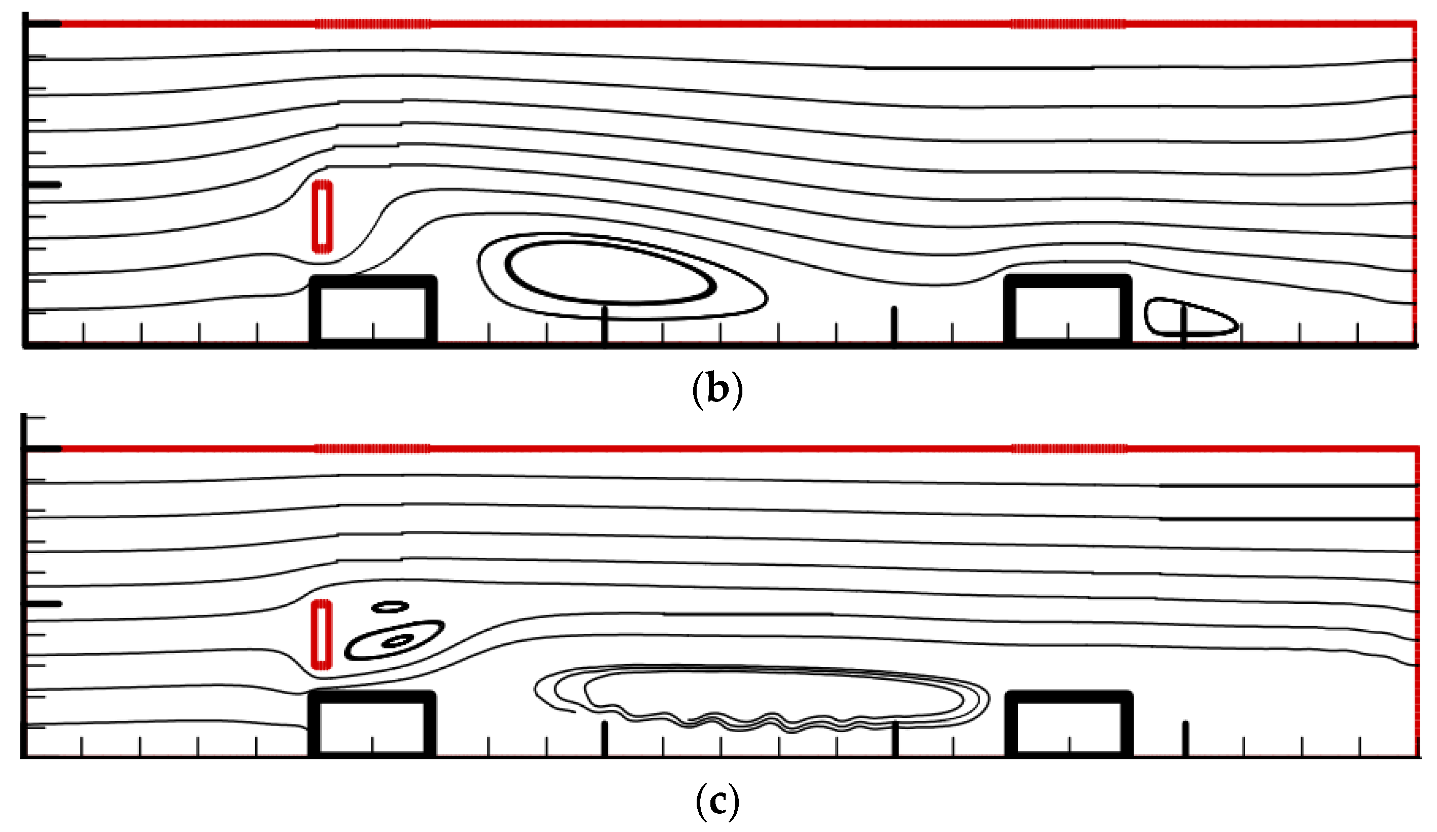
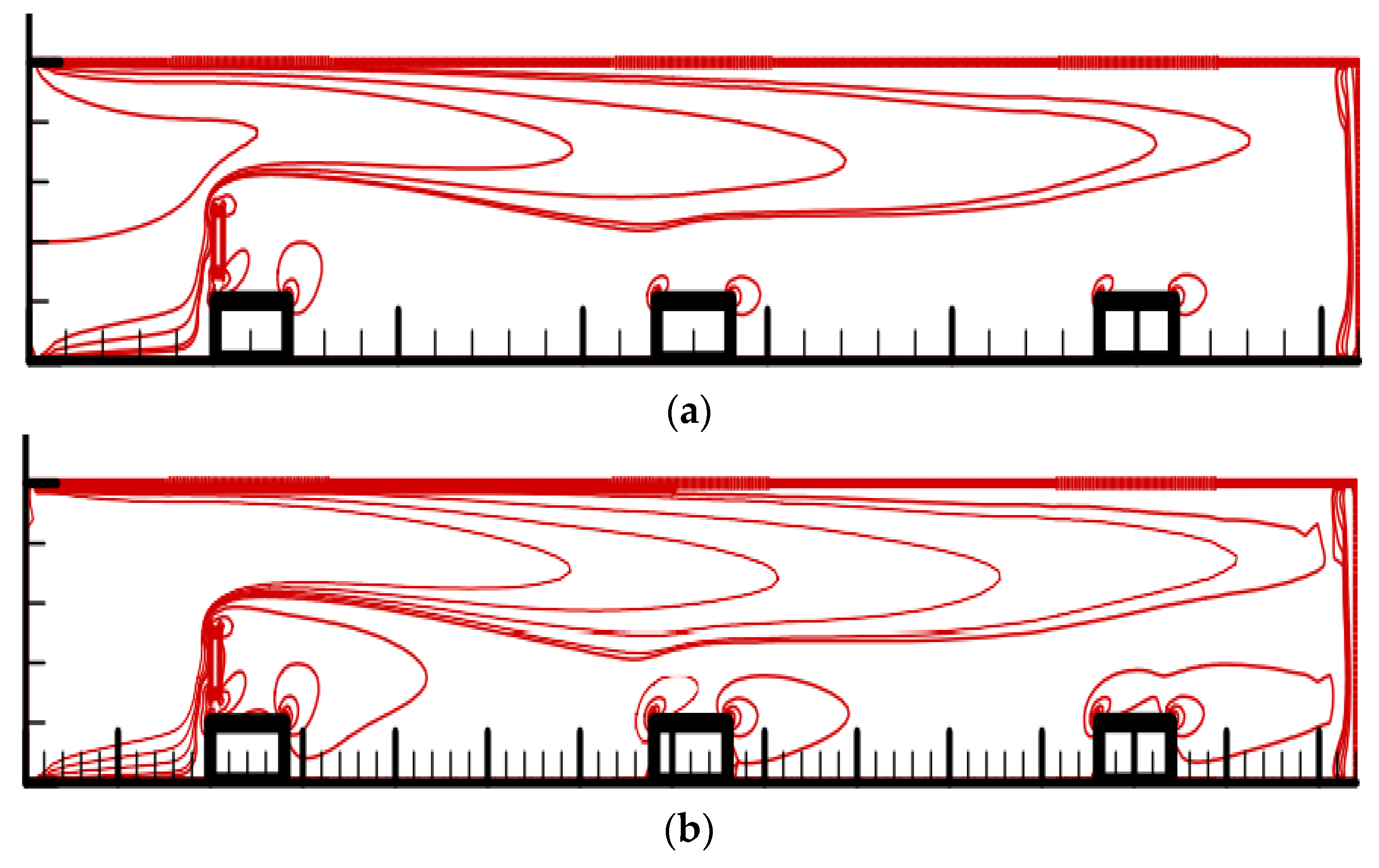
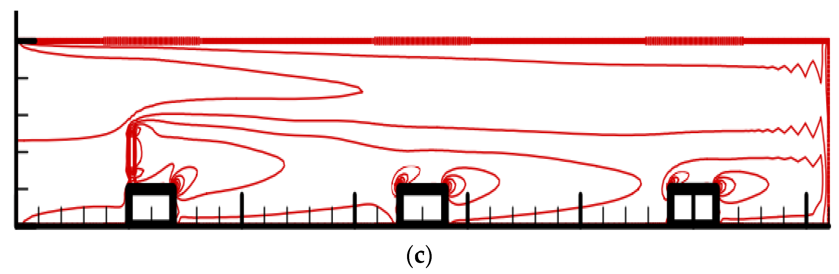
3.4. Streamlined Patterns and Temperature Contours

Figure 5 depicts streamlines for Case 1’s periodic boundary conditions on a heated block at various Reynolds numbers. For each Reynolds number, a recirculation zone forms behind the heated block as the flow passes a rectangular cylinder above each block. Two recirculation zones form behind the rectangular cylinder as the Reynolds number reaches 250 to display a greater streamline curvature on the corners of each heated block. It acquires a higher $\overline{\mathrm{Nu}}$ at a Reynolds number of 250 than at other Reynolds numbers (Figure 2).

Figure 6 shows streamlined patterns for Case 2’s periodic boundary conditions on heated blocks at various Reynolds values. For Reynolds numbers 100 and 175, a substantial recirculation zone arises behind the first heated block when the flow passes a rectangular cylinder above the first block of every two-block case. A smaller recirculation area forms following the second heated block. Two recirculation zones similar to in Case 1 appear behind the rectangular cylinder when the Reynolds number becomes 250, and a large recirculation zone occurs between two heated blocks.

Figure 7 shows streamlines for Case 3’s periodic boundary conditions on heated blocks under different Reynolds numbers. When the fluid flows through a rectangular cylinder above the first block for every three blocks, having a large streamline curvature around the block corner (Figure 7) produces a maximum $\overline{\mathrm{Nu}}$ (Figure 4). A large recirculation zone occurs behind the first heated block, and a smaller recirculation zone appears behind the second and third heated blocks for Reynolds numbers 100 and 175. A big recirculation zone with a smaller recirculation zone forms behind the rectangular cylinder when the Reynolds number is 250. It obtains a higher $\overline{\mathrm{Nu}}$ at a Reynolds number of 250 than other Reynolds numbers (Figure 4). Figure 8 indicates temperature contours for periodic boundary conditions on a heated block for Case 1 at various Reynolds numbers. The distributions of temperature contours for Reynolds numbers are similar; the temperature contours surrounding the first corner (point 1), both ends of the rectangular cylinder, and the second corner (point 3) are denser than those in other areas to cause higher time-mean Nusselt numbers, as shown in Figure 2 (due to a large streamline curvature around the block corner in Figure 5). Figure 9 illustrates temperature contours for periodic boundary conditions on heated blocks for Case 2 under various Reynolds numbers. The distributions of temperature contours for Reynolds numbers are alike; the temperature contours surrounding the corners of each heated block (point 1, point 3, point 6, and point 8) and both ends of the rectangular cylinder are denser than those in other points to cause higher time-mean Nusselt numbers, as shown, in Figure 3 (due to a large streamline curvature around the block corner in Figure 6).

Figure 10 illustrates temperature contours for periodic boundary conditions on heated blocks for Case 3 with variable Reynolds numbers. The distributions of temperature profiles at Reynolds numbers are similar; the temperature contours surrounding the corners of each heated block (point 1, point 3, point 6, point 8, point 11, and point 13) and both ends of the rectangular cylinder are denser than those in other points to cause higher time-mean Nusselt numbers, as shown in Figure 4 (due to a large streamline curvature around the block corner, as shown in Figure 7).

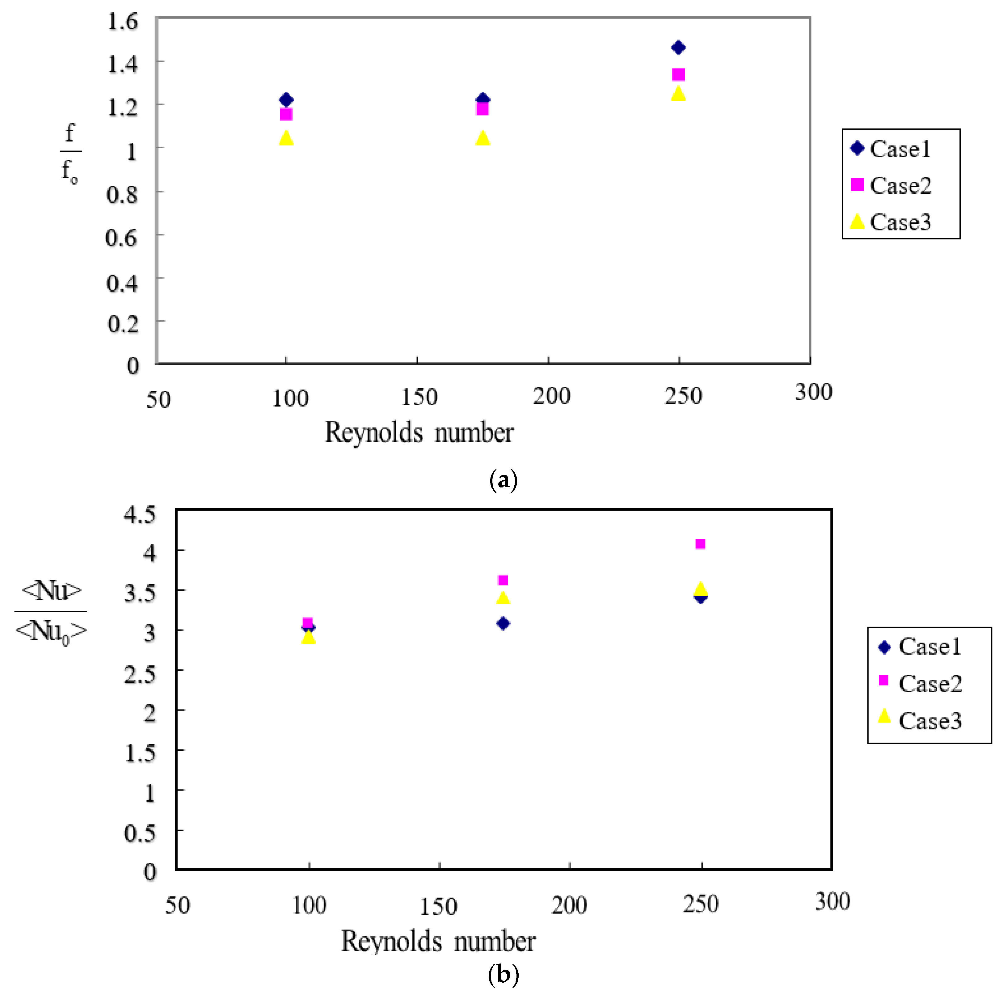
3.5. Friction Factor Enhancement, Nusselt Number Enhancement and Thermal Performance Coefficient

The heated block channel with a rectangular cylinder improves heat transfer and increases flow resistance. A friction factor enhancement $\frac{\mathrm{f}}{{\mathrm{f}}_{\mathrm{o}}}$ reflects the pressure loss ratio between having and not having a rectangular cylinder case, where $\mathrm{f}=△\mathrm{p}/(0.5\mathsf{\rho }{\mathrm{u}}_{\infty }^2)\cdot {\mathrm{d}}_{\mathrm{h}}/\mathrm{L}$ and $f_o$ refers to without rectangular cylinder case. The $\frac{<\mathrm{Nu}>}{{<\mathrm{Nu}}_0>}$ represents Nusselt number enhancement concerning the heat transfer effect between with and without rectangular cylinder case. It is convenient to use Nusselt number enhancement to represent the area average of Nusselt number enhancement in the following. Figure 11 indicates the change in the friction factor enhancement and Nusselt number enhancement with different Reynolds numbers and periodic boundary conditions for various arrangements of rectangular cylinders. The friction factor enhancement $\frac{\mathrm{f}}{{\mathrm{f}}_{\mathrm{o}}}$ indicates Case 1 > Case 2 > Case 3 for Re = 100, 175, and 250. It means that the arrangement of Case 1 produces the highest friction factor enhancement due to the highest pressure drop caused by most fluid contacting surfaces. The area average of time-mean Nusselt number enhancement $\frac{<\mathrm{Nu}>}{{<\mathrm{Nu}}_0>}$ shows Case 2 > Case 3 > Case 1 at Reynolds numbers 175 and 250, and three cases are nearly identical at Re = 100. A coefficient of thermal performance η defined as ($\frac{<\mathrm{Nu}>}{{<\mathrm{Nu}}_0>}/{(\mathrm{f}/{\mathrm{f}}_0)}^{1/3}$) comprises friction factor enhancement and heat transfer enhancement effects to illustrate the combined influence of installing a rectangular cylinder. Figure 12 displays the variance of thermal performance coefficient versus the Reynolds number for periodic boundary conditions under different settings of the rectangular cylinder. Under three Reynolds numbers (100, 175, and 250), the η of Case 2 presents a maximum value, and the η for Case 1 is a minimum. The results imply that a rectangular cylinder above the leading edge of every two heated blocks conducts the best performance, with the rectangular cylinder restraining the fluid flow in Case 2 even more seriously than in Case 3; however, Case 2 performs a much higher heat transfer enhancement than Case 3. Case 1 displays the highest friction factor enhancement and the lowest performance in heat transfer enhancement among the three cases. Therefore, the value order of η follows as Case 2 > Case 3 > Case 1.

4. Conclusions

The study presents three installation cases of a rectangular cylinder for heat transfer enhancement in a heated-block duct under periodic boundary conditions employing the EBE treatment with a semi-implicit projection FEM through a PCG solver. The three cases include rectangular cylinder installation in every block (Case 1), every two blocks (Case 2), and every three blocks (Case 3), to fix a rectangular cylinder for the front corner of the leading block. In these cases, the study analyzes the $\overline{\mathrm{Nu}}$ over the heated-block surface, the streamlines, and the temperature field in the duct under different Reynolds numbers for periodic boundary conditions. The numerical simulation results demonstrate the flow field and thermal convection enhancement of setting a rectangular cylinder within a cooling channel with multiple heated blocks. The distributions of temperature contours for Reynolds numbers are alike; the temperature contours surrounding the corners of each heated block and both ends of the rectangular cylinder are denser than those in other points to cause higher time-mean Nusselt numbers due to a large streamline curvature around the block corner. The difference in thermal performance coefficients in the three permutations provides the total effect of combining convection heat transfer variation and pressure-drop effects. In Case 1, installing too many rectangular cylinders increases the friction factor enhancement due to a higher pressure drop but with enhanced heat transfer due to modifying the flow field of no rectangular cylinder. However, fixing a cylinder every three blocks, as in Case 3, reduces the friction factor enhancement but does not improve heat enhancement like with every two blocks in Case 2. In this study, an appropriate rectangular cylinder arrangement is Case 2 to attain the best thermal performance because it exhibits the highest performance in heat transfer enhancement with a slightly higher friction factor enhancement. The further possible applications of the presented heat transfer enhancement are the cooling problem of multiple heated components such as light-emitting diode modules, printed circuit boards, CPU chips, or heat exchangers to decrease temperature rise effectively and promote use life.

References

1. Ashouri, M.; Ebrahimi, B.; Shafii, M.B.; Saidi, M.H.; Saidi, M.S. Correlation for Nusselt number in pure magnetic convection ferrofluid flow in a square cavity by a numerical investigation. J. Magn. Magn. Mater. 2010, 322, 3607–3613. [Google Scholar] [CrossRef]
2. Dalal, A.; Eswaran, V.; Biswas, G. A finite-volume method for navier-stokes equations on unstructured meshes. Numer. Heat Transf. Part B Fundam. 2008, 54, 238–259. [Google Scholar] [CrossRef]
3. Di Venuta, I.; Boghi, A.; Angelino, M.; Gori, F. Passive scalar diffusion in three-dimensional turbulent rectangular free jets with numerical evaluation of turbulent prandtl/schmidt number. Int. Commun. Heat Mass Transf. 2018, 95, 106–115. [Google Scholar] [CrossRef] [Green Version]
4. Kim, J.; Choi, H.C. An immersed-boundary finite-volume method for simulation of heat transfer in complex geometries. KSME Int. J. 2004, 18, 1026–1035. [Google Scholar] [CrossRef]
5. Hughes, T.J.R.; Levit, I.; Winget, J. Element-by-element implicit algorithms for heat conduction. J. Eng. Mech. 1983, 109, 576–585. [Google Scholar] [CrossRef]
6. Hughes, T.J.R.; Levit, I.; Winget, J. An element-by-element solution algorithm for problems of structural and solid mechanics. Comput. Methods Appl. Mech. Eng. 1983, 36, 241–254. [Google Scholar] [CrossRef]
7. Ortiz, M.; Pinsky, P.M.; Taylor, R.L. Unconditionally stable element-by-element algorithms for dynamic problem. Comput. Methods Appl. Mech. Eng. 1983, 36, 223–239. [Google Scholar] [CrossRef]
8. Winget, J.M. Element by Element Solution Procedures for Nonlinear Transient Heat Condition Analysis. Ph.D. Thesis, California Institute of Technology, Pasadena, CA, USA, 1983. [Google Scholar]
9. Hughes, T.J.R.; Winget, J.; Levit, I.; Tezduyar, T.E. New alternate directions procedure in finite element analysis based upon EBE approximate factorization, Proceedings of the Symposium on Recent Developments in Computer Methods for Nonlinear Solid and Structural Mechanics. In Proceedings of the ASME Joint Meeting of Fluid Engineering, Applied Mechanics and Bioengineering, Houston, TX, USA, 19–22 June 1983; Volume 54, pp. 75–109. [Google Scholar]
10. Hughes, T.J.R.; Raefsky, A.; Muller, A.; Winget, J.; Levit, I. A progress report on EBE solution proceedings in solid mechanics. In Proceedings of the Second International Conference on Nonlinear Problems, Barcelona, Spain, 9–13 April 1984. [Google Scholar]
11. Levit, I. Element-by-element solvers of order N. Comput. Struct. 1987, 27, 357–360. [Google Scholar] [CrossRef]
12. Carey, G.F.; Jiang, B.N. Element-by-element linear and nonlinear solution schemes. Commun. Appl. Numer. Methods 1986, 2, 145–153. [Google Scholar] [CrossRef]
13. Wathen, A.J. An Analysis of some Element-by-element techniques. Comput. Methods Appl. Mech. Eng. 1989, 74, 271–287. [Google Scholar] [CrossRef]
14. Erhel, J.; Traynard, A.; Vidrascu, M. An element-by-Element preconditioned conjugate gradient method implemented on vector computer. Parallel Comput. 1991, 17, 1051–1065. [Google Scholar] [CrossRef]
15. Papadrakakis, M.; Dracopoulos, M.C. A global preconditioner for the element-by-element solution methods. Comput. Methods Appl. Mech. Eng. 1991, 88, 275–286. [Google Scholar] [CrossRef]
16. Mizukami, A. Element-by-element penalty / uzawa formulation for large scale flow problems. Comput. Methods Appl. Mech. Eng. 1994, 112, 283–289. [Google Scholar]
17. Li, Z.; Reed, M.B. Convergence analysis for an element-by-element finite element method. Comput. Methods Appl. Mech. Eng. 1995, 123, 33–42. [Google Scholar] [CrossRef]
18. Sunmonu, A. Implementation of a novel element-by-element finite element method on the hypercube. Comput. Methods Appl. Mech. Eng. 1995, 123, 43–51. [Google Scholar] [CrossRef]
19. Reddy, M.P.; Reddy, J.N. Multigrid methods to accelerate convergence of element-by-element solution algorithms for viscous incompressible flows. Comput. Methods Appl. Mech. Eng. 1996, 132, 179–193. [Google Scholar] [CrossRef]
20. Nakabayashi, Y.; Okuda, H.; Yagawa, G. Parallel finite element fluid analysis on an element-by-element basis. Comput. Mech. 1996, 18, 377–382. [Google Scholar] [CrossRef]
21. Chorin, A.J. Numerical solution of Navier-Stokes equations. Math. Comput. 1968, 22, 745–762. [Google Scholar] [CrossRef]
22. Ramaswamy, B.; Jue, T.C.; Akin, J.E. Semi-implicit and Explicit Finite Element Schemes for Coupled Fluid/Thermal Problems. Int. J. Numer. Methods Eng. 1992, 34, 675–696. [Google Scholar] [CrossRef]
23. Thomas, C.G.; Nithiarasu, P.; Bevan, R.L.T. The locally conservative Galerkin (LCG) method for solving the incompressible Navier-Stokes equations. Int. J. Numer. Methods Eng. 2008, 57, 1771–1792. [Google Scholar] [CrossRef]
24. Savović, S.; Caldwell, J. Finite difference solution of one-dimensional Stefan problem with periodic boundary conditions. Int. J. Heat Mass Transf. 2003, 46, 2911–2916. [Google Scholar] [CrossRef]
25. Murata, H.; Sawada, K.; Suzuki, K. Applicability of spatially periodic boundary conditions to a numerical computation of flow in a channel obstructed by an array of square rods. Heat Transf.-Asia Res. 2004, 33, 357–370. [Google Scholar] [CrossRef]
26. Patankar, S.V.; Liu, C.H.; Sparrow, E.M. Fully developed flow and heat transfer in ducts having streamwise-periodic variation of cross-sectional area. Am. Sot. Mech. Enyrs. Ser. C J. Heat Transf. 1977, 99, 180–186. [Google Scholar] [CrossRef]
27. Gunes, H. Analytical solution of buoyancy-driven flow and heat transfer in a vertical channel with spatially periodic bounda- ry conditions. Heat Mass Transf. 2003, 40, 33–45. [Google Scholar] [CrossRef]
28. Gong, L.; Li, Z.Y.; He, Y.L.; Tao, W.Q. Discussion on numerical treatment of periodic boundary condition for temperature. Numer. Heat Transf. Part B 2007, 52, 429–448. [Google Scholar] [CrossRef]
29. Liou, T.M.; Chang, S.W.; Hung, J.H.; Chiou, S.F. High rotation number heat transfer of a 45° rib-roughened rectangular duct with two channel orientations. Int. J. Heat Mass Transf. 2007, 50, 4063–4078. [Google Scholar] [CrossRef]
30. Liou, T.M.; Chen, S.H.; Shih, K.C. Numerical simulation of turbulent flow field and heat transfer in a two-dimensional channel with periodic slit ribs. Int. J. Heat Mass Transf. 2002, 45, 4493–4505. [Google Scholar] [CrossRef]
31. Xi, W.; Cai, J.; Huai, X. Numerical investigation on fluid-solid coupled heat transfer with variable properties in cross-wavy channels using half-wall thickness multi-periodic boundary conditions. Int. J. Heat Mass Transf. 2018, 122, 1040–1052. [Google Scholar] [CrossRef]
32. Karimian, S.A.M.; Straatman, A.G. A thermal periodic boundary condition for heating and cooling processes. Int. J. Heat Fluid Flow 2007, 28, 329–339. [Google Scholar] [CrossRef]
33. Martinez, E.; Vicente, W.; Salinas-Vazquez, M.; Carvajal, I.; Alvarez, M. Numerical simulation of turbulent air flow on a single isolated finned tube module with periodic boundary conditions. Int. J. Therm. Sci. 2015, 92, 58–71. [Google Scholar] [CrossRef]
34. Debnath, B.; Rao, K.K.; Kumaran, V. Different shear regimes in the dense granular flow in a vertical channel. J. Fluid Mech. 2022, 945, A25. [Google Scholar] [CrossRef]
35. Shim, M.; Ha, M.Y.; Min, J.K. A numerical study of the mixed convection around slanted-pin fins on a hot plate in vertical and inclined channels. Int. Commun. Heat Mass Transf. 2020, 118, 104878. [Google Scholar] [CrossRef]
Figure 1. The geometries for periodic boundary conditions (a) Case 1: with a rectangular cylinder above every block; (b) Case 2: with a rectangular cylinder above the first block for every two blocks; (c) Case 3: with a rectangular cylinder above the first block for every three blocks.
Inventions 08 00097 g001aInventions 08 00097 g001b
Figure 2. Variation in time-mean Nusselt number on a heated block for Case 1 at Re = (a) 100; (b) 175; (c) 250. Numbers: the point along the heated block surface.
Inventions 08 00097 g002
Figure 3. Variation in time-mean Nusselt number on heated blocks for Case 2 at Re = (a) 100; (b) 175; (c) 250. Numbers: the point along the heated blocks surfaces.
Inventions 08 00097 g003
Figure 4. Variation in time-mean Nusselt number on heated blocks for Case 3 at Re = (a) 100; (b) 175; (c) 250. Numbers: the point along the heated blocks surfaces.
Inventions 08 00097 g004
Figure 5. Streamline patterns for periodic boundary conditions on a heated block for Case 1 at Re = (a) 100; (b) 175; (c) 250. Red: recangular cylinder; Black: heated block.
Inventions 08 00097 g005
Figure 6. Streamline patterns for periodic boundary conditions on a heated block for Case 2 at Re = (a) 100; (b) 175; (c) 250.
Inventions 08 00097 g006aInventions 08 00097 g006b
Figure 7. Streamline patterns for periodic boundary conditions on heated blocks for Case 3 at Re = (a) 100; (b) 175; (c) 250.
Inventions 08 00097 g007aInventions 08 00097 g007b
Figure 8. Temperature contours for periodic boundary conditions on a heated block for Case 1 at Re = (a) 100; (b) 175; (c) 250.
Inventions 08 00097 g008
Figure 9. Temperature contours for periodic boundary conditions on heated blocks for Case 2 at Re = (a) 100; (b) 175; (c) 250.
Inventions 08 00097 g009
Figure 10. Temperature contours for periodic boundary conditions on heated blocks for Case 3 at Re = (a) 100; (b) 175; (c) 250.
Inventions 08 00097 g010aInventions 08 00097 g010b
Figure 11. (a) Variation in friction factor enhancement; (b) Variation in Nusselt number enhancement with Reynolds number for periodic boundary conditions with various arrangements of rectangular cylinders.
Inventions 08 00097 g011
Figure 12. Variation in thermal performance with Reynolds number for periodic boundary conditions with various arrangements of rectangular cylinders.
Inventions 08 00097 g012