Article

A Generalized Framework for Adopting Regression-Based Predictive Modeling in Manufacturing Environments

by
Mobayode O. Akinsolu
1,2,* and
Khalil Zribi
1,3
1
Faculty of Arts, Science and Technology, Wrexham Glyndŵr University, Wrexham LL11 2AW, UK
2
Academic Engagement Department, The Alan Turing Institute, British Library, London NW1 2DB, UK
3
ESEO Angers—Grande Ecole d’Ingénieurs Généralistes, 10 Bd Jean Jeanneteau, 49100 Angers, France
*
Author to whom correspondence should be addressed.
Inventions 2023, 8(1), 32; https://doi.org/10.3390/inventions8010032
Submission received: 14 December 2022 / Revised: 7 January 2023 / Accepted: 20 January 2023 / Published: 29 January 2023
(This article belongs to the Collection Feature Innovation Papers)

Abstract

:
In this paper, the growing significance of data analysis in manufacturing environments is exemplified through a review of relevant literature and a generic framework to aid the ease of adoption of regression-based supervised learning in manufacturing environments. To validate the practicality of the framework, several regression learning techniques are applied to an open-source multi-stage continuous-flow manufacturing process data set to typify inference-driven decision-making that informs the selection of regression learning methods for adoption in real-world manufacturing environments. The investigated regression learning techniques are evaluated in terms of their training time, prediction speed, predictive accuracy (R-squared value), and mean squared error. In terms of training time ( T T ), k-NN20 (k-Nearest Neighbour with 20 neighbors) ranks first with average and median values of 4.8 ms and 4.9 ms, and 4.2 ms and 4.3 ms, respectively, for the first stage and second stage of the predictive modeling of the multi-stage continuous-flow manufacturing process, respectively, over 50 independent runs. In terms of prediction speed ( P S ), DTR (decision tree regressor) ranks first with average and median values of 5.6784 × 10 6 observations per second (ob/s) and 4.8691 × 10 6 observations per second (ob/s), and 4.9929 × 10 6 observations per second (ob/s) and 5.8806 × 10 6 observations per second (ob/s), respectively, for the first stage and second stage of the predictive modeling of the multi-stage continuous-flow manufacturing process, respectively, over 50 independent runs. In terms of R-squared value ( R 2 ), BR (bagging regressor) ranks first with average and median values of 0.728 and 0.728, respectively, over 50 independent runs, for the first stage of the predictive modeling of the multi-stage continuous-flow manufacturing process, and RFR (random forest regressor) ranks first with average and median values of 0.746 and 0.746, respectively, over 50 independent runs, for the second stage of the predictive modeling of the multi-stage continuous-flow manufacturing process. In terms of mean squared error ( M S E ), BR (bagging regressor) ranks first with average and median values of 2.7 and 2.7, respectively, over 50 independent runs, for the first stage of the predictive modeling of the multi-stage continuous-flow manufacturing process, and RFR (random forest regressor) ranks first with average and median values of 3.5 and 3.5, respectively, over 50 independent runs, for the second stage of the predictive modeling of the multi-stage continuous-flow manufacturing process. All methods are further ranked inferentially using the statistics of their performance metrics to identify the best method(s) for the first and second stages of the predictive modeling of the multi-stage continuous-flow manufacturing process. A Wilcoxon rank sum test is then used to statistically verify the inference-based rankings. D T R and k-NN20 have been identified as the most suitable regression learning techniques given the multi-stage continuous-flow manufacturing process data used for experimentation.

1. Introduction

As the world continues to gravitate to artificial intelligence (AI)-driven societies, where paradigms such as Industry 4.0 [1] and Society 5.0 [2] are gradually and increasingly redefining the manufacturing and production of goods and services, and how we live and interact, respectively, the role of the science of data in the drive for innovation and invention cannot be overemphasized [3,4]. Presently, AI, which in a sense premises on data-driven models and constructs [5], is one of the primary proponents of Industry 4.0 (I4.0) and Industry 5.0 (I5.0) [3]. With a focus on manufacturing, from the first industrial revolution in the 1760s to the present-day I4.0 and I5.0, manufacturing across the globe has always involved workflows and processes that churn out vast amounts of data [3,4]. For example, timestamps and time logs on machine tools and equipment, sensor readings, operational speeds of rotating tools, and measurements of throughput and slags on shop floors have always generated vast amounts of data [6,7]. As a matter of fact, this in a way idealizes big data, where manufacturing big data can be broadly described as data collected at every stage of manufacturing and/or production, including data from operators, equipment, machine tools, process systems, and devices on the shop floor [8,9].
As hinted at above, manufacturing has always been data intensive. However, up until recent times, manufacturing data has not really been used to “automagically” improve or enhance the manufacturing processes that generated them in the first place [9,10]. In other words, other than process monitoring and regulation that are mostly achieved via traditional process visualization and process control using human-machine interfaces (HMIs), manufacturing data is still yet to be used extensively to support data-driven paradigms such as predictive modeling (usually takes the form of predictive maintenance when machine behavior and the life cycle is the context [11,12]) and ubiquitous monitoring and control (usually incorporated in the industrial internet of things (IIoT) where higher levels of connectivity, interoperability and robustness is the goal [13,14]). This apparent gap can be mainly attributed to the purpose-built or fit-for-purpose nature of most of the computational paradigms and analytic frameworks that support manufacturing processes [5].
To lend credence to the above-mentioned, the example of a manufacturing or production process can be used. Take, for instance, a programmable logic controller (PLC) designated for overseeing the operations of a conveyor belt system using a master-slave (M-S) architecture that only needs to power the motor of the conveyor belt system on and/or off based on some measured metrics such as read sensor values when the conveyed item reaches a designated point or landmark along the production line as exemplified in [15]. In a sense, every other data such as the remaining useful life (RUL) of the motor and quality of the product (the item being conveyed in this case such as the bottles and trays in [15]) that are also associated with the process may not really impact on the modi operandi of the PLC-based M-S control architecture. However, if such data are made available and analyzed, inferences drawn from such analysis can go a long way in improving the overall efficiency of the process. Consequently, it is to this end that data science is more relevant than it has ever been before in ushering in a new era of data-driven innovations and inventions in manufacturing environments.
It can be argued that many of the data-driven innovations and inventions expected to be seen in the global manufacturing sector will be mostly based on predictive modeling [3,5,16]. Generally, predictive modeling can be viewed as being synonymous with supervised learning, a form of machine learning or subcategory of AI that can take on the form of classification and/or regression, depending on the nature or type of data that is employed. For most commercial applications, particularly, manufacturing applications as discussed in [17], predictive modeling can also be called predictive analytics. Broadly speaking, predictive analytics is the analysis of available data (e.g., explanatory and response variables in a typical manufacturing process data set as carried out in Section 2.3) and data trends using statistical learning and/or machine learning methods to enable and support the prediction of future trends and/or responses. According to the literature, the global manufacturing industry can be said to be in the early stage of adopting AI in many of their production processes, particularly, machine learning in the form of predictive modeling [5,16]. So, this has necessitated the conceptualization, design, development, and testing of several paradigms by scientists, engineers, and researchers as also carried out in this work.
Presently, contemporary manufacturing technologies now support the embedding of predictive modeling and other AI-based paradigms into many manufacturing and production processes [18,19,20]. Some of these manufacturing processes include, but are not limited to, maintenance planning, quality control, monitoring and regulation, and robust automation of shop floor operations [18,19,20]. Hence, there is a growing need to have a generic framework that supports the holistic and granular use of data sets from manufacturing processes to support data-driven innovations and inventions in manufacturing environments. To respond to this need, a generalized framework is presented and investigated in this paper to support predictive modeling in manufacturing environments. More specifically, the following contributions are made:
  • Formulation of a generalized framework for predictive modeling in manufacturing environments using data collected from real-time manufacturing processes.
  • Validation of the proposed generalized framework by applying several regression learning techniques to undertake predictive modeling using an open-source multi-stage continuous-flow manufacturing process data set.
  • Summarized inference-based and statistically verified rankings for the adoption and selection of regression learning techniques to potentially invent predictive modeling-based paradigms for typical manufacturing processes.
The remainder of this paper is organized as follows: Section 2.1 provides a summarized discussion on the relevant related work to further emphasize the usefulness of the work carried out. Section 2.2 details the proposed generalized framework and the main steps required for its implementation. An overview of the case study used to validate the proposed generalized framework is provided in Section 2.3, alongside a description of the associated multi-stage continuous-flow manufacturing process data set. The machine learning problem addressed by the proposed framework in the context of the adopted case study, and the investigated algorithms are detailed in Section 2.4. The experimental setup used for the investigations is presented in Section 3. Results, discussions, and comparisons are detailed in Section 4, and the concluding remarks are provided in Section 5.

2. Materials and Methods

2.1. Relevant Related Work

Machine learning (ML) in the form of data-driven predictive modeling in manufacturing environments is gaining a lot of research interest in recent times [18,19,20]. Regression or regression analysis or regression learning is one of the widely accepted approaches for predictive modeling in many contexts, including manufacturing [21]. For example, in [7], a generic data analytics system is proposed and demonstrated to be viable for manufacturing production systems. Inventory forecasting, product evaluation, and machine tool condition monitoring are some of the use cases adopted in [7]. For these use cases, manufacturing tasks such as time-series prediction, rules extraction, and general prediction were adequately accomplished. However, in contrast to the work carried out in this paper where several machine learning methods have been investigated, only three machine learning methods were reported on in [7], as part of the experiments and investigations conducted. These methods are random forest, multilayer perceptron, and generalized linear model. Even though these three machine learning methods are arguably among the widely used and popular machine learning methods, there are several other widely-used and popular machine learning methods such as the ones investigated in this paper.
To efficiently evaluate carbon emission from manufacturing processes, particularly machining in manufacturing shop floors and/or workshops, a big data analysis approach involving a data-driven multi-level assessment is proposed in [8] as another instance of adopting ML in manufacturing environments. The work carried out and reported in [8] primarily involves three core stages that provide adequate insights into the pre-processing, correlation analysis, and multi-level data-driven formulation of evaluation indicators or responses of production state data from typical manufacturing shop floors or workshops. Note that the essential steps such as the cleansing of the manufacturing data, partitioning of the manufacturing processes, reduction of the manufacturing data, and extraction of features from the manufacturing data are all adequately captured and detailed in [8], as essential components of the proposed big data analysis approach. However, in contrast to the work presented in this paper, predictive modeling was not explicitly undertaken as part of the big data analysis approach in the manufacturing contexts detailed in [8].
More recently, to have more effective and efficient planning, scheduling, and management with predictive maintenance and product quality in multistage manufacturing or production systems comprising batching machines and finite buffers, a data-driven quantitative method is proposed in [22]. The method proposed in [22] premises on a decision model represented by a Markov decision process whose optimal maintenance policy is desired to satisfy Bellman’s optimality equation. To overcome the dimensionality curse and solve the optimality equation, approximate dynamic programming implemented using a deep Q-network algorithm is employed in [22]. Even though the work carried out in [22] adequately and dynamically quantifies the impact of machine breakdowns, maintenance actions, and quality failures on manufacturing or production, only one algorithm was investigated and predictive modeling was not thoroughly explored to make a strong case for harnessing its potential in manufacturing environments in areas such as forecasting and trend analysis of manufacturing or production processes.
Similar work to the endeavor in [22] was reported in [10]. As a supposed improvement on the work carried out in [22], the exploration of optimal maintenance policies also represented by a Markov decision process is further augmented by considering machine stoppage bottlenecks on the shop or plant floors. To do this, two approaches involving the improvement of the worst machine and a random machine, respectively, were considered with a focus on the reduction of the downtime duration. Even though machine stoppage bottlenecks were considered alongside numerical analysis involving comparisons with popular and widely accepted methods by manufacturers in [10] in addition to the work carried out in [22], the drawback of not thoroughly exploring the potential of predictive modeling to make a strong case for its adoption, given the manufacturing and/or production context investigated remains. Hence, this can still be viewed arguably as a relatively grey area of research interest considering the potential impact of the adoption of predictive modeling in manufacturing or production environments.
Therefore, it is observed that currently, the available literature does not offer an in-depth investigative study where several machine learning algorithms or techniques are utilized in the same context to make a strong case for their adoption in predictive modeling in manufacturing environments. For example in [20], only five methods are investigated to make a case for optimal pick-and-place process controls that enhance the efficiency and quality of surface mount technology. The research investigations presented in this paper are devoted to this end, i.e., the investigation of multiple machine learning methods to make a case for their potential adoption in typical manufacturing processes and/or environments.

2.2. The Proposed Framework

The flow diagram of the proposed generalized framework for the adoption of regression learning in manufacturing environments investigated in this work is shown in Figure 1. The framework is both suitable for dynamic and/or static inflows of manufacturing data and some of the steps are iterative. In the context of this work, dynamic data is defined as data collected instantaneously and recursively from manufacturing processes and utilized on the fly for data-driven predictive modeling. In this way, the model is updated continuously and it feeds back, directly, to the manufacturing processes that produced the data used for its construction. It is envisaged that such a model can be employed for trend analysis and predictive maintenance in manufacturing environments. In contrast to dynamic data, static data in the context of this work is also defined as data collected instantaneously from manufacturing processes; however, it is not utilized on the fly for data-driven predictive modeling.
To better distinguish between dynamic data and static data in this work, as already explained above, it is good to note that in practice, the first step to undertaking real-world predictive modeling is to utilize static data (as defined above) to build models that can predict responses from manufacturing processes. These models are then fine-tuned and thoroughly evaluated in terms of predictive accuracy, uncertainty, and other performance metrics before they are deployed for on-the-fly data-driven predictive modeling using dynamic data (as defined above). To validate the proposed framework, an open-source multi-stage continuous-flow manufacturing process data set has been used as an initial step to showcase its feasibility. Even though the multi-stage continuous-flow manufacturing process data set has been generated by collecting data and information from dynamic manufacturing processes [23], the models built using the data have not been deployed in real-world manufacturing environments for paradigms such as trend analysis and predictive maintenance. So, the framework proposed and investigated in this work primarily serves as a precursor to real-world physical implementation. The essential steps are described summarily as follows:
  • Step 1: Data is collected instantaneously and/or recursively from critical manufacturing processes of interest. The collected data is used to create a database, M D B .
  • Step 2: Metrics for all explanatory and response variables in M D B , E D B and R D B , respectively, are passed through purpose-built functions to generate a clean database, M D B C = [ E D B C , R D B C ], where unwanted observations or data (e.g., redundant data) are handled correctly and robustly. See Section 2.3.1 for more details on the custom functions adopted in this work.
  • Step 3: Since the metrics in M D B C are expected to be from the continuous-flow stages of manufacturing processes, M D B C is grouped to ensure metrics collected from the same stage of the manufacturing process are collocated. For example, M D B C 1 (first stage) and M D B C 2 (second stage) for a two-stage continuous-flow manufacturing process as we have investigated in this work (See Section 2.3).
  • Step 4: Exploratory data analysis techniques are employed for the univariate analysis and multivariate analysis of the metrics in M D B C to establish their descriptive statistics and relationships. In this work, only descriptive statistics are presented.
  • Step 5: The explanatory metrics in M D B C (i.e., E D B C ) are then normalized for regression learning to have a new database (i.e., E D B n o r m C as carried out in this work (See Section 2.4)).
  • Step 6: Predictive modeling is carried out by applying several regression learning techniques to [ E D B n o r m C , R D B C ] to ascertain the most suitable ones in terms of the mean squared error ( M S E ), predictive accuracy (R-squared value ( R 2 )), prediction speed ( P S ), and training time ( T T ).
  • Step 7: To rank all methods, some inferences are drawn a posteriori based on the assessment of the outcomes from Step 6.
  • Step 8: The inference-based rankings from Step 7 are statistically verified to determine the best regression learning technique(s) to select and adopt for the given manufacturing process data set.
More details about the implementation of the proposed framework are presented in Section 2.3, Section 2.4 and Section 3, where the case study involving an open-source multi-stage continuous-flow manufacturing process data set is further described [23], the procedures in all the steps summarized above are detailed, and the experimental setup is presented, respectively. Note that, for such a data-driven paradigm concocted by the proposed framework, the end product will be a software application that is deployed either as an add-on or a toolbox for existing manufacturing process automation, monitoring, and control software applications. Naively, the software application can be fed data (mostly from sensors interfaced and integrated with the manufacturing process as described in Section 2.3) and using this data, it implements the steps described above for the proposed framework to build and select near-optimal regression learning models for the behavioral analysis and predictive modeling of the manufacturing process that generated its input data. The behavioral analysis and predictive modeling of the manufacturing process can then be adopted for predictive maintenance, trend analysis, and optimal tuning of the manufacturing process.

2.3. Case Study of a Multi-Stage Continuous-Flow Manufacturing Process

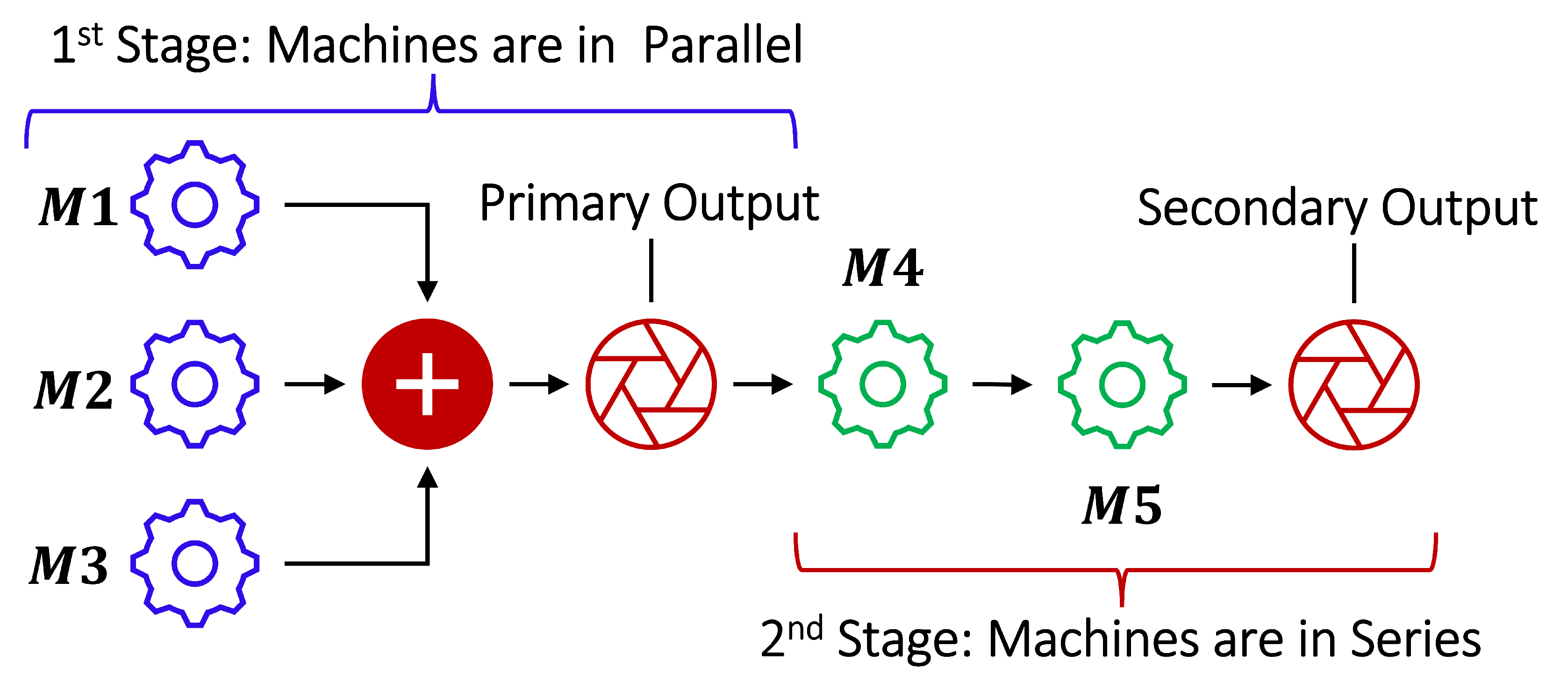
A case study involving a multi-stage continuous-flow manufacturing process is used to validate the proposed framework in Section 2.2 and the architecture of the manufacturing process is shown in Figure 2. In contrast to batch production or manufacturing process, the materials being processed in this case study are constantly in motion on the shop floor along the production or manufacturing process line. The main elements of the multi-stage continuous flow manufacturing process are five operational machines ( M 1 , M 2 , M 3 , M 4 , and M 5 ) and a combiner ( C O M B ) that are employed in two stages (see Figure 2). Sensors have been used for data (temperature, pressure, speed, and others) collection [23]. Some of the data collected include (but are not limited to) factory ambient conditions, temperature, pressure, speed, and amperage of the machines. Since the goal of our work is to primarily report on predictive modeling, the manufacturing process and the manufacturing environment used as the case study have not been extensively discussed. However, more details about the manufacturing process and manufacturing environment can be found in [23] or by contacting [24].
Considering the fact that the data collected from the two-stage continuous-flow manufacturing process is over a four-hour operational window, in comparison to the operational hours of real-world manufacturing processes, this may be viewed as being relatively short in some contexts, e.g., continuous manufacturing where the production lines are operational all the time and the available manufacturing process data can be infinitely large. The operating conditions may also be assumed to be relatively stable due to the minimal or no noise observed in the collected data set. In reality, the operational window would be longer and unstable conditions may be observed from time to time, for example, due to mechanical vibrations, and friction noise, after long operational hours of rotating equipment such as motors. Be that as it may, the four-hour operational window can still be argued to emulate the multi-stage continuous-flow manufacturing process reasonably well based on the half-hour to five-hour sampling window recommended in [25] for modeling a typical manufacturing process.
To deploy data-driven predictive modeling systems in real-world manufacturing scenarios, only a subset of the manufacturing data is used per time (and not an infinitely large data set) due to limitations in hardware and computing resources, standard data augmentation techniques can then be employed to extrapolate the data collected over relatively short operational times to account for longer operational hours and better capture the dynamics of the shop floors. Noisy data can be both studied and generated synthetically from the big data to mirror or model current and potential noise patterns in the data set to better account for unstable conditions that may stem from mechanical vibrations and others, after long hours of operation. These approaches require additional studies, investigations, experiments, and possibly a miniaturized manufacturing process model (for example, a model such as the PETRA II [26]) to validate their practicality. Since this is beyond the scope of the work presented in this paper, studies, investigations, and experiments, in this regard, are neither presented nor discussed in this work.
With a focus on the data components of the two-stage continuous flow manufacturing process, the first stage comprises three machines ( M 1 , M 2 , and M 3 ) that operate in parallel to constitute the parallel stage of the multi-stage continuous flow manufacturing process. M 1 , M 2 , and M 3 each have eight process variables to account for properties such as temperature, speed, pressure, amperage, and others. The outputs from M 1 , M 2 , and M 3 are fed into a step that combines the flows. This combiner stage for M 1 , M 2 , and M 3 has three process variables associated with it) and its output is the primary controlled output. The primary controlled output is measured at 15 unique locations. The combined output from the first stage is then fed to the second stage of the continuous-flow manufacturing process. The second stage comprises two machines ( M 4 and M 5 ) that operate in series to constitute the series stage of the multi-stage continuous-flow manufacturing process. M 4 and M 5 each have seven process variables to also account for properties such as temperature, speed, pressure, amperage, and others. The output from the second stage is the secondary controlled output and it is also measured at 15 unique locations. The process variables and the controlled outputs used for generating the data set are further discussed in Section 2.3.1.

2.3.1. Data Set Description

The data used for the experimentation and investigations come from a single production or manufacturing process run spanning several hours. Large quantities of this type of data are available from [24], and they are often collected from multiple production lines in various locations to mitigate bias and support the generalization of the data set. In our experiments, a total of over 14,000 observations have been used. If each observation ( 0 i ) is defined as a proper subset of the set, M D B C (database of the clean data (see Section 2.2)), such that i∈ [1,…, 14,088], the data set can be described mathematically as follows:
0 i M D B C
where M D B C is generated from the data cleaning process detailed as follows:
1
For every observation in M D B , select all the columns for the explanatory variables to have an array or matrix E D B and select all the columns for the response variables to have an array or matrix R D B .
2
For every column vector ( E D B j ) in E D B , perform the following operations:
E D B C = Obtain the mode of E D B j Store as E M o d e Determine the frequency of E M o d e in E D B j Store as E F r e q . If E F r e q . T H O L D remove E D B j from E D B Otherwise keep E D B j in E D B
3
For every column vector ( R D B j ) in R D B , perform the following operations:
R D B C = Obtain the mode of R D B j Store as R M o d e Determine the frequency of R M o d e in R D B j Store as R F r e q . If R F r e q . T H O L D remove R D B j from R D B Otherwise keep R D B j in R D B
where T H O L D is set to be equal to 6000 and M D B C = { E D B C , R D B C } .
Note that by setting T H O L D = 6000 in Equations (2) and (3), if any metric is repeated for 6000 times or more (i.e., representing 40% or more) in any column of the metrics for the explanatory and response variables, such a variable is assumed to be fairly constant and discarded (not included in the data set). After the data cleaning operations, the variables in M D B C are mathematically described as follows for any ith observation having explanatory variables 0 i E and response variables 0 i R in M D B C :
0 i E = { F A C 1 , F A C 2 } ; Factory ambient conditions . { M 1 P V 1 , M 1 P V 2 , M 1 P V 3 , M 1 P V 4 , M 1 P V 5 , M 1 P V 6 , M 1 P V 7 , M 1 P V 8 } ; M 1 process variables . { M 2 P V 1 , M 2 P V 2 , M 2 P V 3 , M 2 P V 4 , M 2 P V 5 , M 2 P V 6 , M 2 P V 7 , M 2 P V 8 } ; M 2 process variables . { M 3 P V 1 , M 3 P V 2 , M 3 P V 3 , M 3 P V 4 , M 3 P V 5 , M 3 P V 6 , M 3 P V 7 , M 3 P V 8 } ; M 3 process variables . { T C O M B 1 , T C O M B 2 , T C O M B 3 } ; Combiner stage process variables for M 1 , M 2 and M 3 . { M 4 P V 1 , M 4 P V 2 , M 4 P V 3 , M 4 P V 4 , M 4 P V 5 , M 4 P V 6 , M 4 P V 7 } ; M 4 process variables . { M 5 P V 1 , M 5 P V 2 , M 5 P V 3 , M 5 P V 4 , M 5 P V 5 , M 5 P V 6 , M 5 P V 7 } ; M 5 process variables .
0 i R = { S 1 C O 1 , S 1 C O 2 , S 1 C O 3 , S 1 C O 4 , S 1 C O 5 , S 1 C O 6 , S 1 C O 7 , S 1 C O 8 , S 1 C O 9 , S 1 C O 10 , S 1 C O 11 , S 1 C O 12 , S 1 C O 13 , S 1 C O 14 , S 1 C O 15 } ; Primary controlled output . { S 2 C O 1 , S 2 C O 2 , S 2 C O 3 , S 2 C O 4 , S 2 C O 5 , S 2 C O 6 , S 2 C O 7 , S 2 C O 8 , S 2 C O 9 , S 2 C O 10 , S 2 C O 11 , S 2 C O 12 , S 2 C O 13 , S 2 C O 14 , S 2 C O 15 } ; Secondary controlled output .
From Equations (4) and (5), it can be seen that there are a total of 43 explanatory variables and 30 response variables. For the predictive modeling of the primary controlled output, the factory ambient conditions (i.e., [ F A C 1 , F A C 2 ]), the process variables of M 1 , M 2 and M 3 (i.e., [ M 1 P V 1 ,…, M 1 P V 8 ], [ M 2 P V 1 ,…, M 2 P V 8 ], and [ M 3 P V 1 ,…, M 3 P V 8 ], respectively) and the combiner stage process variables (i.e., [ T C O M B 1 , T C O M B 2 , T C O M B 3 ]) are the explanatory variables, and the primary controlled output (i.e., [ S 1 C O 1 ,…, S 1 C O 15 ]) is the response to be predicted. The descriptive statistics for these variables are given in Table 1 and Table 2. For the predictive modeling of the secondary controlled output, the factory ambient conditions (i.e., [ F A C 1 , F A C 2 ] and the process variables of M 4 and M 5 (i.e., [ M 4 P V 1 ,…, M 4 P V 7 ], and [ M 5 P V 1 ,…, M 5 P V 7 ], respectively) are the explanatory variables, and the secondary controlled output (i.e., [ S 2 C O 1 ,…, S 2 C O 15 ]) is the response. The descriptive statistics for these variables are given in Table 1 and Table 2.
From the values reported in Table 1 and Table 2, it can be said that the explanatory and response variables all have a significant spread. This is an indication that for every 0 i , the elements all have values that are not necessarily close to their means (i.e., expected values) which are spread over a wider range. To improve the performance and training stability of the regression models to be built using the variables described in Table 1 and Table 2, it is essential to transform the features (i.e., specifically, the explanatory variables described in Table 1) to be on a similar scale. In this work, normalization, a popular machine learning approach has been used and it is discussed as follows:

Feature Scaling of the Data Set

Feature scaling is a widely used data pre-processing procedure in machine learning when supervised learning techniques such as regression and classification are employed [27,28]. It is often carried out through the normalization of the range of the explanatory variables or independent variables (also called features) in the data set. Normalization mainly guarantees that the numerical weights contributed approximately and proportionally to the responses or targets by each explanatory variable (feature) are relatively similar [28]. In this way, data redundancy is minimized and the variables have an agreeable metric scale.
In a typical machine learning process, feature scaling can be implemented in a number of ways [27,28]. For example, z-scores as carried out in [29] and min-max linear transformation as carried out in [30,31]. In this work, feature scaling has been implemented on the explanatory variables (see Equation (4) and its description) using a min-max linear transformation (normalization) as follows:
E D B n o r m C R i = E D B C R i E D B m i n C R i E D B m a x C R i E D B m i n C R i
where E D B C R i is the ith metric in the data column for the Rth variable in E D B C whose minimum and maximum values are E D B m i n C R i and E D B m a x C R i , respectively, and E D B n o r m C R i is the normalized value defined as E D B n o r m C R i [ 0 , 1 ] . After the normalization, the transformed data set ( M D B n o r m C ) can be described mathematically as follows:
M D B n o r m C = { E D B n o r m C , R D B C }

2.4. The Machine Learning Problem and Investigated Methods

In this work, several specialized machine learning methods (including methods having similar model construction methodologies but different hyperparameter settings or control parameter settings) that support outputting multiple response variables for each prediction are investigated. These algorithmic methods are demonstrated to be practical and useful for undertaking predictive modeling in manufacturing environments as exemplified in this work. Using the context of the case study presented in Section 2.3, predictive modeling problem definition, feature scaling of the data set, regression learning, and summarized description of the investigated machine learning methods are detailed as follows:

2.4.1. Predictive Modeling Problem Definition for the Case Study

Briefly, predictive modeling can be best described as a paradigm that adopts both machine learning and data mining techniques to predict or forecast some target data or responses given a set of observations. Considering the case study presented in Section 2.3, to predict the manufacturing process line’s outputs (i.e., [ S 1 C O 1 ,…, S 1 C O 15 ] for the first stage and [ S 2 C O 1 ,…, S 2 C O 15 ] for the second stage), machine learning methods or algorithms that adequately support multi-target data are required. Intuitively, this is because the manufacturing process data set (as described in Section 2.3) contains multi-target data from the two stages (see Figure 2). Note that multi-target learning subsumes many machine learning problems in several disciplines and handles complex decision-making in many real-world applications such as manufacturing processes.
The complexity of multi-target learning mainly stems from its intrinsic multivariate nature that yields complex interactions between its multiple explanatory and response variables. These interactions have not been investigated in this work as exemplified in [30] using typical explanatory variables because it is not within the scope of the work carried out. However, since both the explanatory and response variables in M D B n o r m C are continuous variables (see Table 1 and Table 2, and Section 2.3), regression learning-based predictive modeling must be employed to address the machine learning problem. This is the focus of the work carried out in this paper and regression learning for the case study is discussed in Section 2.4.2 as follows:

2.4.2. Regression Learning for the Case Study

Regression learning is a widely used supervised learning technique for machine learning-based predictive modeling [32]. As a data-driven methodology, it generally takes the form of linear regression analysis for the conventional analysis of data [33]. Primarily, it is used for forecasting outcomes in a methodical and mathematical way that sorts the impact of the independent feature(s) or variable(s) on the associated dependent response(s) or variable(s) in any given data set. The regression learning implementation in this work can be mathematically described as follows for the two stages of the continuous-flow manufacturing process:
S 1 C O m i = f ( F A C n o r m i n , M 1 P V n o r m i n , M 2 P V n o r m i n , M 3 P V n o r m i n , T C O M B n o r m i n , β ) + e i
S 2 C O m i = f ( F A C n o r m i n , M 4 P V n o r m i n , M 5 P V n o r m i n , β ) + e i
In Equation (8), S 1 C O m i m = [ 1 , , 15 ] , F A C n o r m i n = [ 1 , 2 ] , M 1 P V n o r m i n = [ 1 , , 8 ] , M 2 P V n o r m i n = [ 1 , , 8 ] , M 3 P V n o r m i n = [ 1 , , 8 ] , T C O M B n o r m i n = [ 1 , 2 , 3 ] , β and e i are the primary controlled outputs, normalized factory ambient conditions, normalized process variables for M 1 , normalized process variables for M 2 , normalized process variables for M 3 , normalized process variables for the combiner stage of M 1 , M 2 , and M 3 , unknown parameters (usually, scalar coefficients) and error terms (usually, scalar), respectively, for the ith observation in M D B n o r m C . m is the total number of occurrences of the primary controlled output in M D B n o r m C and n is the total number of process variables from the factory ambient conditions, each of M 1 , M 2 , and M 3 , and the combiner stage for M 1 , M 2 , and M 3 . Equation (8) is then used to predict S 1 C O for new or arbitrary values of F A C n o r m , M 1 P V n o r m , M 2 P V n o r m , M 3 P V n o r m and T C O M B n o r m . In Equation (9), S 2 C O m i m = [ 1 , , 15 ] , F A C n o r m i n = [ 1 , 2 ] , M 4 P V n o r m i n = [ 1 , , 8 ] , M 5 P V n o r m i n = [ 1 , , 8 ] , β and e i are the secondary controlled outputs, normalized factory ambient conditions, normalized process variables for M 4 , normalized process variables for M 5 , respectively, for the ith observation in the M D B n o r m C . m is the total number of occurrences of the secondary controlled output in M D B n o r m C and n is the total number of process variables from the factory ambient conditions and each of M 4 and M 5 . Equation (9) is then used to predict S 2 C O for new or arbitrary values of F A C n o r m , M 4 P V n o r m , and M 5 P V n o r m .
It is good to note that all the machine learning methods investigated in this work have been applied for regression learning, in consonance with the multi-stage continuous-flow manufacturing process data set described in Section 2.3.1. In other words, they have been used for regression analysis. As a result, their respective approximate computational complexities have been estimated using the context of a typical linear regression algorithm. The implementation of linear regression mainly focuses on finding a solution to the matrix or linear algebra problem described as follows:
( Y Y ) 1 × ( Y Z )
where Y is the matrix holding the predictors or explanatory variables or independent variables and it is a (14,088 × 29) matrix and a (14,088 × 16) matrix for the first stage and second stage of the predictive modeling of the multi-stage continuous-flow manufacturing process, respectively, as discussed in Section 2.3.1. Y is the transpose of Y, and Z is the matrix holding the responses or target variables, or independent variables. Z is a (14,088 × 15) matrix for both the first and second stages of the predictive modeling of the multi-stage continuous-flow manufacturing process.
For the first stage of the predictive modeling of the multi-stage continuous-flow manufacturing process, Y holds the metrics of the factory ambient conditions (i.e., [ F A C 1 , F A C 2 ]) and the following process variables (see Table 1): [ M 1 P V 1 ,…, M 1 P V 8 ], [ M 2 P V 1 ,…, M 2 P V 8 ], [ M 3 P V 1 ,…, M 3 P V 8 ] and [ T C O M B 1 , T C O M B 2 , T C O M B 3 ]. For the second stage of the predictive modeling of the multi-stage continuous-flow manufacturing process, Y holds the metrics of the factory ambient conditions (i.e., [ F A C 1 , F A C 2 ]) and the following process variables (see Table 1): [ M 4 P V 1 ,…, M 4 P V 7 ], and [ M 5 P V 1 ,…, M 5 P V 7 ]. For the first stage of the predictive modeling, Z holds the metrics of the primary output to control, i.e., [ S 1 C O 1 ,…, S 1 C O 15 ] (see Table 2). For the second stage of the predictive modeling of the multi-stage continuous-flow manufacturing process, Z holds the metrics of the secondary output to control, i.e., [ S 2 C O 1 ,…, S 2 C O 15 ] (see Table 2).
By examining Equation (10) and the dimensions of Y and Z, respectively, the matrix product Y × Y can be estimated to have a complexity of O ( 29 2 × 14,088 ) and O ( 16 2 × 14,088 ) for the first stage and second stage of the predictive modeling of the multi-stage continuous-flow manufacturing process, respectively. The inverse operation of ( Y × Y ) 1 can be estimated to have a complexity of O ( 29 3 ) and O ( 16 3 ) for the first stage and second stage of the predictive modeling of the multi-stage continuous-flow manufacturing process, respectively. The product Y × Z can be estimated to have a complexity of O ( 29 × 14,088 ) and O ( 16 × 14,088 ) for the first stage and second stage of the predictive modeling of the multi-stage continuous-flow manufacturing process, respectively. Hence, the overall computational complexity can be estimated to be O ( 14,088 × 29 2 + 29 3 ) and O ( 14,088 × 16 2 + 16 3 ) for the first stage and second stage of the predictive modeling of the multi-stage continuous-flow manufacturing process, respectively. As such for any M n total number of observations from the manufacturing process having any M p metrics, the computational complexity may be generalized and estimated as follows:
O ( M n × M p 2 + M p 3 )
where M n and M p will assume their values according to the given linear regression problem.
The regression learning methods or regression techniques investigated in this work are listed in Table 3 and references are also provided for their full descriptions. These methods include variants of multi-output regression (MOR) in which different regression algorithms have been used as estimators and k-nearest neighbors (k-NN) where the implementation is carried out using four different values of k, 1, 5, 10, and 20 to have N N , k-NN5, k-NN10 and k-NN20, respectively.

3. Experimental Setup

For the implementation of all the machine learning methods, Scikit-learn library [36,54] and Google Colaboratory development environment [55] have been used. Specifically, the investigated algorithms have been coded using the library functions available from [36,54]. All the settings for the hyperparameters or control parameters for the respective methods are the Scikit-learn library’s default settings, except where stated otherwise. The assumption made is that these default settings in the Scikit-learn library are unlikely to be altered by most manufacturing engineers, not experienced in machine learning. Conventionally, most machine learning methods or algorithms show better performance if and/or when their hyperparameters or control parameters are tuned or optimized [56,57]. However, since this is not the aim of this work, this has not been investigated.
In this work, some exceptions regarding hyperparameter tuning investigations can be found in methods such as k-NN (k-nearest neighbor), where different values have been used for the number of neighbors to have different approaches for the same method. Other methods such as RF (random forest) and SVR (support vector regression) that can be argued not to naturally support multi-target regression have been fitted using the multi-output regressor (MOR) in the Scikit-learn library to have different adaptations (or tuning, naively) to allow for multi-target regression using different approaches with similar underlying frameworks. These methods can also be viewed as an exception in terms of hyperparameter tuning. To examine the predictive accuracy of the fitted models from all methods, the validation scheme used is hold-out validation. The choice of this validation scheme is guided by the total number of observations (more than 14,000 (see Section 2.3)). Following some popular approaches for typical hold-out validation schemes [58], 70% of the observations have been used as the training data set and the remaining 30% have been used as the test data set for all experiments.
To compare the regression models built and trained by all methods, the training time ( T T ), prediction speed ( P S ), predictive accuracy (R-squared value ( R 2 )), and mean squared error ( M S E ) of all methods are used over 50 independent statistical runs. In each independent run, a regression model is built and trained for each of the methods investigated. Note that the 50 independent runs allow for statistical inference and analysis, and comparisons of the efficiencies and robustness of the investigated methods in terms of their performance metrics ( T T , P S , R 2 , and M S E ). Also, by having a sample size of 50, hypothesis tests for probability estimation using a z-statistic can be carried out (See Section 4). All experiments have been carried out on a workstation with Intel 4-core i7-4770K 3.50 GHz CPU and 24.0 GB RAM, except where stated otherwise. Elapsed times reported are elapsed real times from a wall clock.

4. Results and Discussion

In this section, the results of all methods are presented, discussed, and compared in terms of T T , P S , R 2 , and M S E . The comparisons are made to establish the most suitable method for each stage of the predictive modeling of the multi-stage continuous-flow manufacturing process. The methods are ranked inferentially using their performance metrics ( T T , P S , R 2 , and M S E ) from their independent runs, and the rankings are statistically verified for validation.

4.1. Training Time

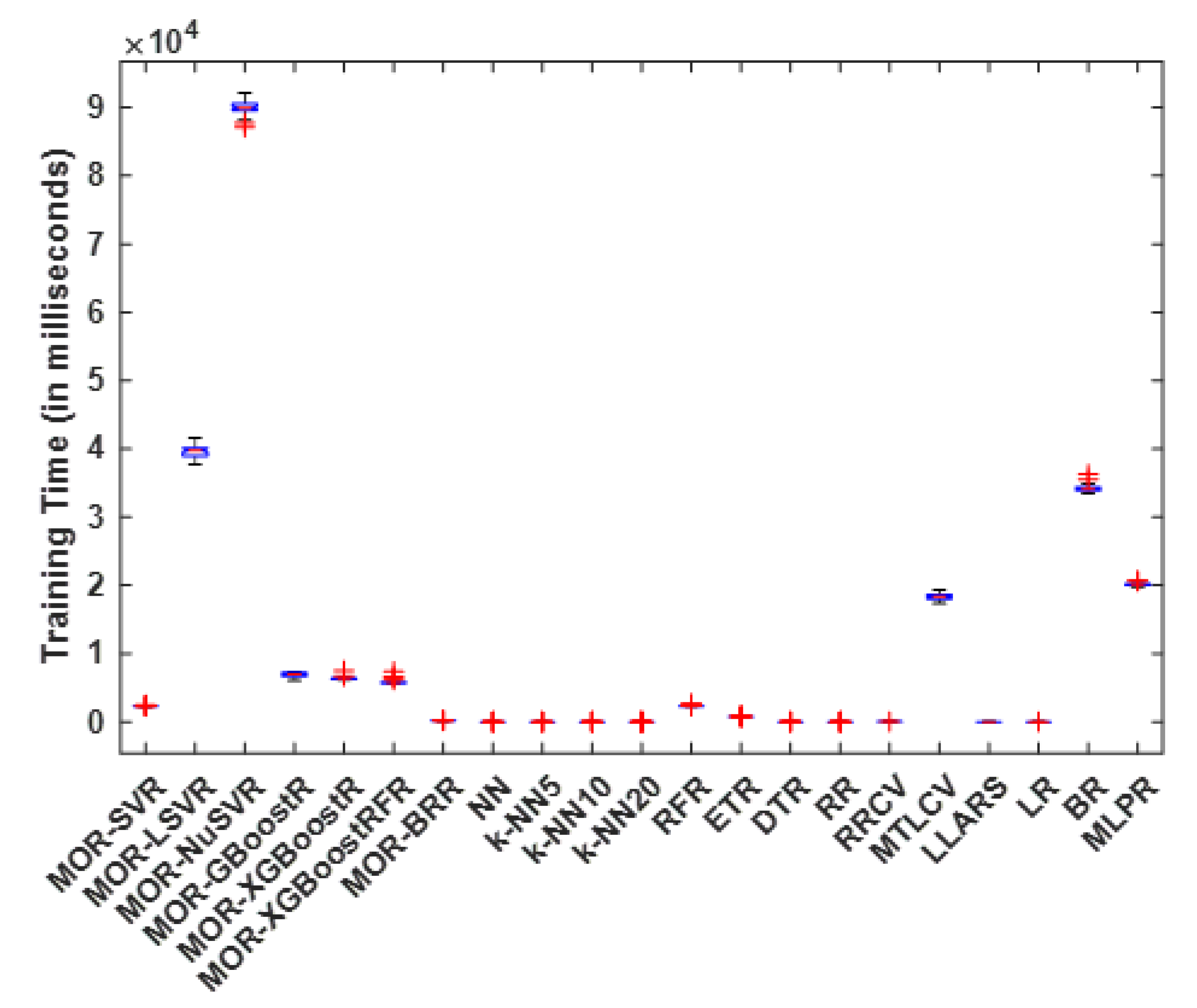
In regression learning, the training time ( T T ) can be best described as the time taken to build and train a regression model. T T is typically measured in seconds or fractions of seconds (e.g., milliseconds, microseconds, nanoseconds, etc.). From Table 4, the following observations are made for the T T of all methods for the first stage of the predictive modeling of the multi-stage continuous-flow manufacturing process: (1) The T T of all methods are generally lower than 120 s on average. (2) k-NN20 shows the best average and median T T of 4.8 ms and 4.9 ms, respectively, over the 50 independent runs. (3) The average and median T T for NN and k-NN10 (4.9 ms and 5.0 ms, and 5.0 ms and 5.1 ms, respectively) over the 50 independent runs are also short and comparable to those of k-NN20. (4) MTLCV shows the worst average and median T T of 60,883.6 ms and 60,837.8 ms, respectively, over the 50 independent runs. (5) The average and median T T for BR and MLPR (58,489.6 ms and 58,287.5 ms, and 42,700.9 ms and 42,682.0 ms, respectively) over the 50 independent runs are also long. (6) The robustness of the methods is relative according to their standard deviations over all runs: k-NN10 has the lowest standard deviation of 0.3 and MTLCV has the highest standard deviation of 2035.8. So, in terms of T T stability for the first stage of the predictive modeling of the multi-stage continuous-flow manufacturing process, k-NN10 can be said to be the most robust among all the methods, while MTLCV is the least robust. The box plots of T T for all the methods are shown in Figure 3, for the first stage of the predictive modeling of the multi-stage continuous-flow manufacturing process. The findings earlier discussed can be corroborated visually by an examination of the variations in T T for all the methods in Figure 3.
In a similar vein to the discussion above for Table 4 and Figure 3, the following observations are made from Table 5 for the T T of all methods for the second stage of the predictive modeling of the multi-stage continuous-flow manufacturing process: (1) The T T of all methods are generally lower than 91 s on average. (2) k-NN20 shows the best average and median T T of 4.2 ms and 4.3 ms, respectively, over the 50 independent runs. (3) The average and median T T for k-NN10, k-NN5, and NN (4.4 ms and 4.4 ms, 4.5 ms and 4.5 ms, and 4.5 ms and 4.5 ms, respectively) over the 50 independent runs are also short and comparable to those of k-NN20. (4) MOR-NuSVR shows the worst average and median T T of 90,015.0 ms and 89,941.3 ms, respectively, over the 50 independent runs. (5) The average and median T T for MOR-LSVR and BR (39,647.9 ms and 39,768.1 ms, and 34,183.6 ms and 34,043.4 ms, respectively) over the 50 independent runs are also long. (6) The robustness of the methods is relative according to their standard deviations over all runs: k-NN5 and k-NN10 have the lowest standard deviation of 0.2 and MOR-LSVR has the highest standard deviation of 983.8. So, in terms of T T stability for the second stage of the predictive modeling of the multi-stage continuous-flow manufacturing process, k-NN5 and k-NN10 can be said to be the most robust among all the methods, while MOR-LSVR is the least robust. The box plots of T T for all the methods are shown in Figure 4, for the second stage of the predictive modeling of the multi-stage continuous-flow manufacturing process. The findings earlier discussed can be corroborated visually by an examination of the variations in T T for all the methods in Figure 4.

4.2. Prediction Speed

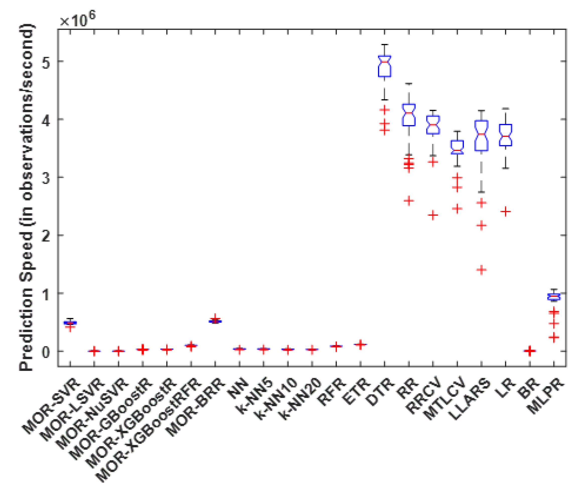
Generally, in machine learning, the prediction speed ( P S ) of a method is derived as the total number of predictions made by a method divided by the time taken to make the predictions. It is measured in observations per second (obs/s). The P S of all methods for the first stage of the predictive modeling of the multi-stage continuous-flow manufacturing process is reported in Table 6. From Table 6, the following observations are made for P S : (1) The P S of all methods are generally higher than 90 obs/s on average. (2) DTR shows the best average and median P S of 4.8691 × 10 6 obs/s and 4.9929 × 10 6 obs/s, respectively, over the 50 independent runs. (3) The average and median P S for RR and RRCV ( 4.0102 × 10 6 obs/s and 4.1101 × 10 6 obs/s, and 3.8520 × 10 6 obs/s and 3.9050 × 10 6 obs/s, respectively) over the 50 independent runs are also fast. (4) MOR-NuSVR shows the worst average and median P S of 9.2834 × 10 1 obs/s and 9.2775 × 10 1 obs/s, respectively, over all 50 independent runs. (5) The average and median T T for MOR-LSVR and BR ( 1.4115 × 10 2 obs/s and 1.4085 × 10 2 obs/s, and 3.4633 × 10 3 obs/s and 3.4946 × 10 3 obs/s, respectively) over the 50 independent runs are also slow. (6) The robustness of all the methods is relative according to their standard deviations over all runs: MOR-NuSVR has the lowest standard deviation of 2.1876 and RR has the highest standard deviation of 3.9870 × 10 5 . So, in terms of P S stability for the first stage of the predictive modeling of the multi-stage continuous-flow manufacturing process, MOR-NuSVR can be said to be the most robust among all the methods, while RR is the least robust. The box plots of P S for all the methods are shown in Figure 5, for the first stage of the predictive modeling of the multi-stage continuous-flow manufacturing process. The findings earlier discussed can be corroborated visually by an examination of the variations in P S for all the methods in Figure 5.
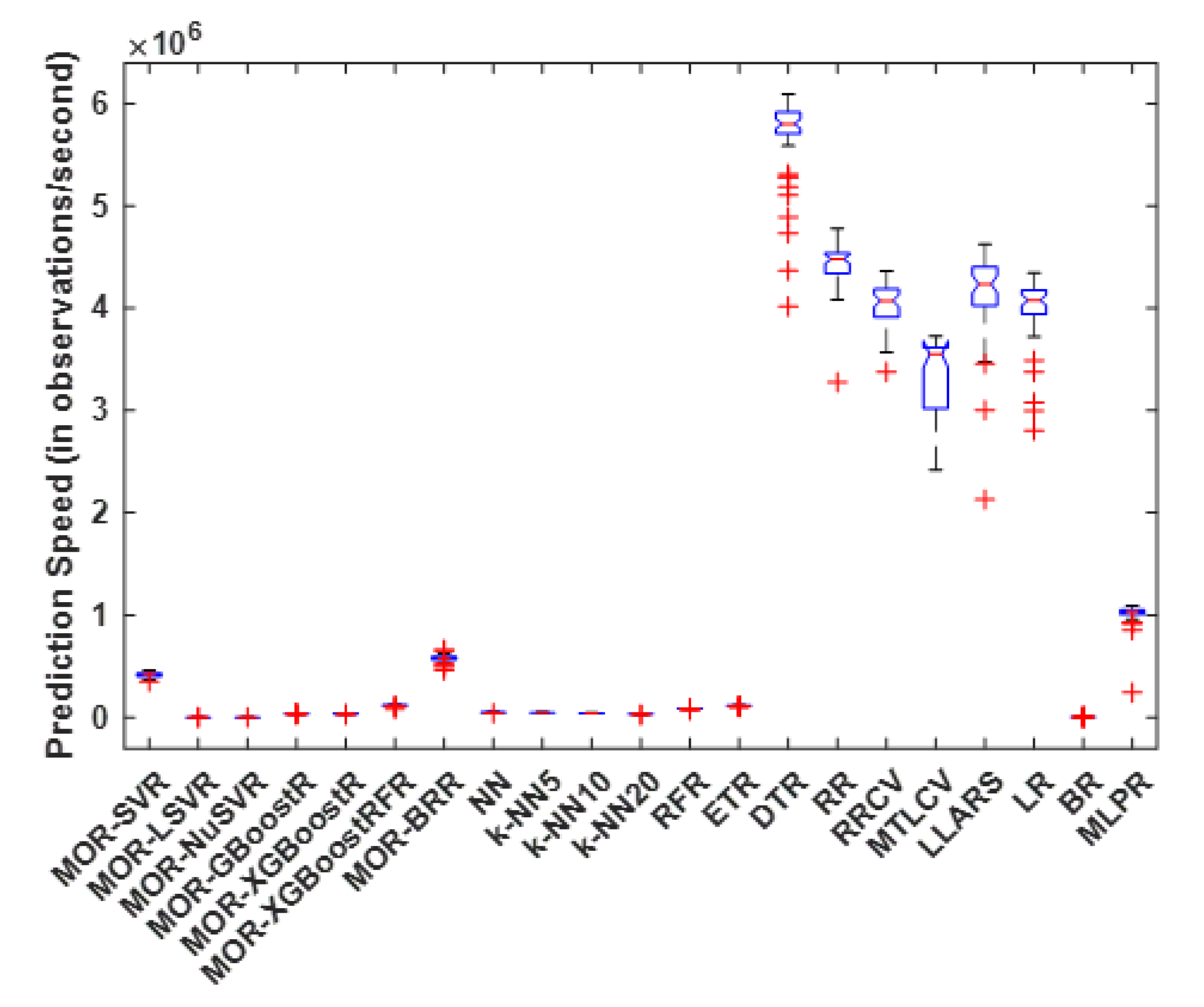
In a similar vein to the discussion above for Table 6 and Figure 5, the following observations are made from Table 7 for the P S of all methods for the second stage of the predictive modeling of the multi-stage continuous-flow manufacturing process: (1) The P S of all methods are generally higher than 130 obs/s on average. (2) DTR shows the best average and median P S of 5.6784 × 10 6 obs/s and 5.8007 × 10 6 obs/s, respectively, over the 50 independent runs. (3) The average and median P S for RR and LLARS ( 4.4236 × 10 6 obs/s and 4.1231 × 10 6 obs/s, and 4.4792 × 10 6 obs/s and 4.2340 × 10 6 obs/s, respectively) over the 50 independent runs are also fast and comparable. (4) MOR-NuSVR shows the worst average and median P S of 1.3128 × 10 2 obs/s and 1.3213 × 10 2 obs/s, respectively, over the 50 independent runs. (5) The average and median T T for MOR-LSVR and BR ( 1.7654 × 10 2 obs/s and 1.7680 obs/s, and 3.5747 × 10 3 obs/s and 3.5933 × 10 3 obs/s, respectively) over the 50 independent runs are also slow. (6) The robustness of all methods is relative according to their standard deviations over all runs: MOR-NuSVR has the lowest standard deviation of 2.7050 and LLARS has the highest standard deviation of 4.4958 × 10 5 . So, in terms of P S stability for the second stage of the predictive modeling of the multi-stage continuous-flow manufacturing process, MOR-NuSVR can be said to be the most robust among all the methods, while LLARS is the least robust. The box plots of P S for all the methods are shown in Figure 6, for the second stage of the predictive modeling of the multi-stage continuous-flow manufacturing process. The findings earlier discussed can be corroborated visually by an examination of the variations in P S for all the methods in Figure 6.

4.3. R-Squared Statistic

In machine learning, the R-squared value or statistic ( R 2 ) is also called the coefficient of determination and it helps to estimate the goodness of the fit of regression models. In regression learning, it can be derived as follows:
R 2 = S S R S S T = 1 S S E S S T
where S S R is the sum of squares regression, S S E is the sum of squares residual error, and S S T is the sum of squares total. In Equation (12), R 2 [ 0 , 1 ] , indicating that R 2 typically takes on a value between null and unity (i.e., 0% and 100%), where R 2 = 0 indicates that the regression model explains none of the variability of the response data around its mean and R 2 = 1 indicates that the model explains all the variability of the response data around its mean. In other words, the higher the R 2 value of the regression model, the better the regression model fits the data (in this case the multi-stage continuous-flow manufacturing process data). Note that for some methods, R < 0 holds when the regression model is arbitrarily worse. Methods that yielded such models in our experiments have not been presented in this work due to their non-suitability.
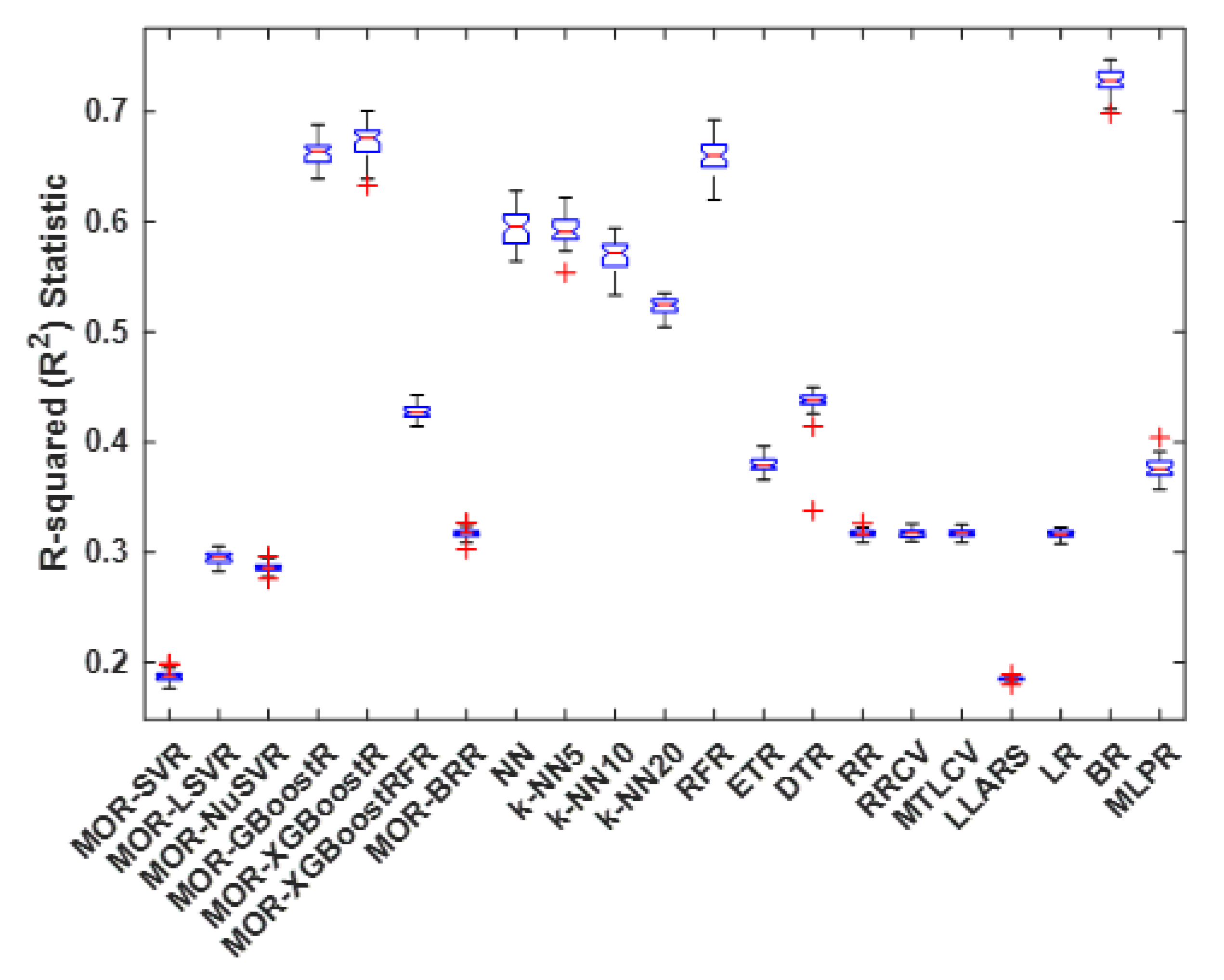
The R 2 of all methods for the first stage of the predictive modeling of the multi-stage continuous-flow manufacturing process is reported in Table 8. From Table 8, the following observations are made for R 2 : (1) The R 2 of all methods are generally higher than 0.18 on average. (2) BR shows the best average and median R 2 of 0.728 and 0.728, respectively, over the 50 independent runs. (3) The average and median R 2 for MOR-XGBoostR and MOR-GBoostR (0.673 and 0.676, and 0.663 and 0.664, respectively) over the 50 independent runs are also relatively high and comparable. (4) LLARS shows the worst average and median R 2 of 0.185 and 0.185, respectively, over the 50 independent runs. (5) The average and median R 2 for MOR-SVR and MOR-NuSVR (0.188 and 0.188, and 0.286 and 0.286, respectively) over the 50 independent runs are also small. (6) All methods show relatively good robustness according to their standard deviations over all runs: LLARS has the lowest standard deviation of 0.002 and NN has the highest standard deviation of 0.016. So, in terms of R 2 stability for the first stage of the predictive modeling of the multi-stage continuous-flow manufacturing process, LLARS can be said to be the most robust among all the methods, while NN is the least robust. The box plots of R 2 for all the methods are shown in Figure 7, for the first stage of the predictive modeling of the multi-stage continuous-flow manufacturing process. The findings earlier discussed can be corroborated visually by an examination of the variations in R 2 for all the methods in Figure 7.
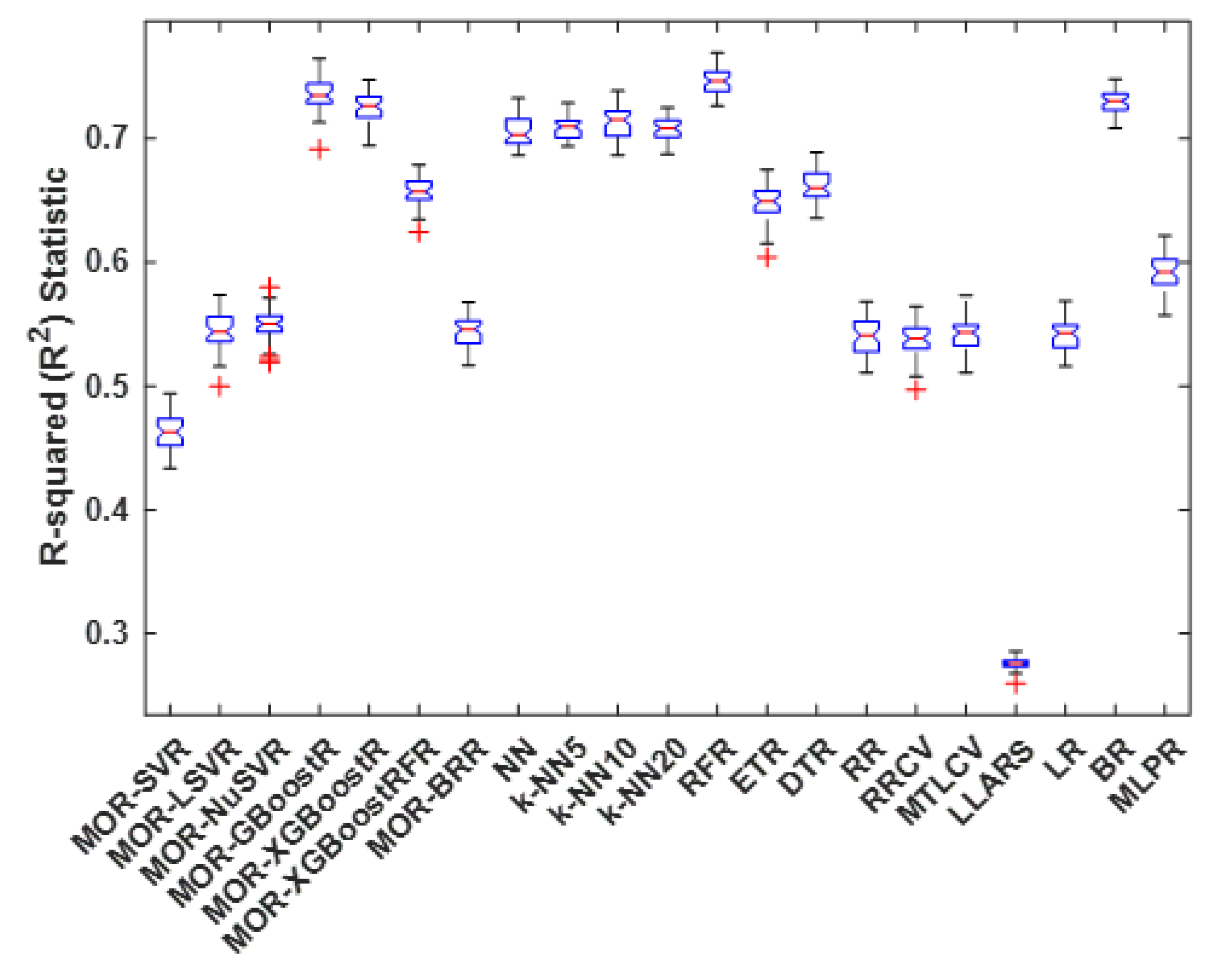
In a similar vein to the discussion above for Table 8 and Figure 7, the following observations are made from Table 9 for the R 2 of all methods for the second stage of the predictive modeling of the multi-stage continuous-flow manufacturing process: (1) The R 2 of all methods are generally higher than 0.53 on average. (2) RFR shows the best average and median R 2 of 0.746 and 0.746, respectively, over the 50 independent runs. (3) The average and median R 2 for MOR-GBoostR and MOR-XGBoostR (0.736 and 0.735, and 0.726 and 0.726, respectively) over the 50 independent runs are also high and comparable to those of RFR. (4) LLARS shows the worst average and median R 2 of 0.275 and 0.276, respectively, over the 50 independent runs. (5) The average and median R 2 for MOR-SVR (0.463 and 0.463, respectively) over the 50 independent runs are also small in comparison to other methods. (6) All methods show relatively good robustness according to their standard deviations over all runs: LLARS has the lowest standard deviation of 0.005 and MOR-SVR, MOR-LSVR, and RR have the highest standard deviation of 0.015 each. So, in terms of R 2 stability for the second stage of the predictive modeling of the multi-stage continuous-flow manufacturing process, LLARS can be said to be the most robust among all the methods, while MOR-SVR, MOR-LSVR, and RR are the least robust. The box plots of R 2 for all the methods are shown in Figure 8, for the second stage of the predictive modeling of the multi-stage continuous-flow manufacturing process. The findings earlier discussed can be corroborated visually by an examination of the variations in R 2 for all the methods in Figure 8.

4.4. Mean Squared Error

The mean squared error ( M S E ) is another statistical measure used in machine learning to evaluate regression learning models. Mathematically, the M S E of a regression model is the average squared difference between the predicted values by the model and the observed values. In regression learning, it can be derived as follows:
M S E = 1 n i = 1 n ( Y i Y i ^ ) 2
where n is the number of observations, Y i and Y i ^ are the actual value and estimated or predicted value, respectively, for the ith observation in the data set. Note that in regression learning, M S E is always positive or greater than null such that M S E 0 depicts the better quality of the regression model and M S E = 0 indicates that the regression model is a perfect predictor.
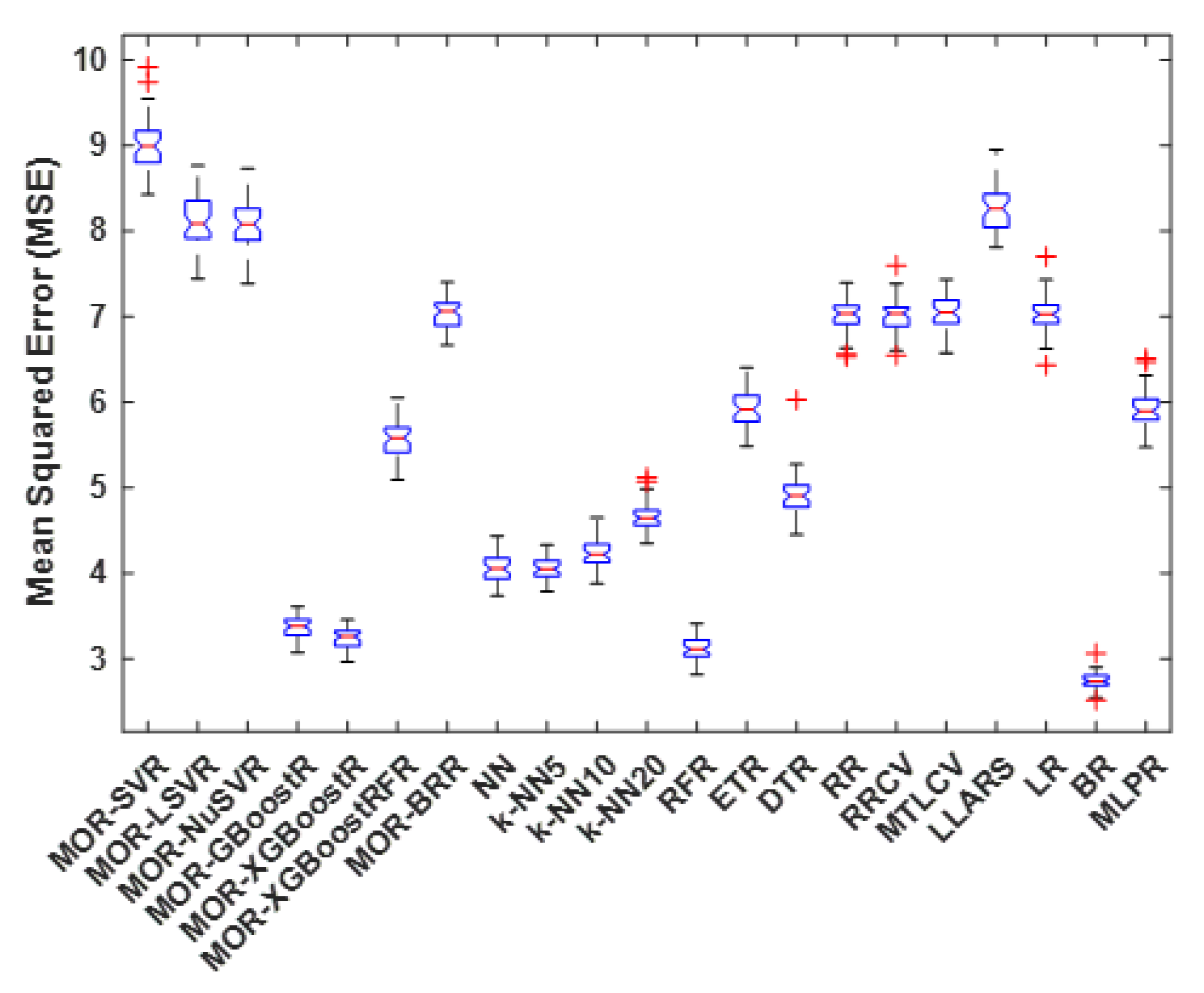
The M S E of all methods for the first stage of the predictive modeling of the multi-stage continuous-flow manufacturing process is reported in Table 10. From Table 10, the following observations are made for the M S E : (1) The M S E of all methods are generally higher than 2.5 on average. (2) BR shows the best average and median M S E of 2.7 and 2.7, respectively, over the 50 independent runs. (3) The average and median M S E for MOR-XGBoostR and MOR-GBoostR (3.2 and 3.3, and 3.4 and 3.4, respectively) over the 50 independent runs are also low and comparable. (4) MOR-SVR shows the worst average and median M S E of 9.0 and 9.0, respectively, over the 50 independent runs. (5) The average and median M S E for LLARS (8.3 and 8.3, respectively) over the 50 independent runs are also high and comparable to those of MOR-LSVR and MOR-NuSVR (8.1 and 8.1, respectively, for both methods). (6) The robustness of all methods is relative according to their standard deviations over all runs: MOR-GBoostR, MOR-XGBoostR, k-NN5, k-NN10, RFR and BR have the least standard deviation of 0.1, while MOR-SVR and MOR-LSVR have the highest standard deviation of 0.3. So, in terms of M S E stability for the first stage of the predictive modeling of the multi-stage continuous-flow manufacturing process, MOR-GBoostR, MOR-XGBoostR, k-NN5, k-NN10, RFR and BR can be said to be the most robust among all the methods, while MOR-SVR and MOR-LSVR are the least robust. The box plots of M S E for all the methods are shown in Figure 9, for the first stage of the predictive modeling of the multi-stage continuous-flow manufacturing process. The findings earlier discussed can be corroborated visually by an examination of the variations in M S E for all the methods in Figure 9.
In a similar vein to the discussion above for Table 10 and Figure 9, the following observations are made from Table 11 for the M S E of all methods for the second stage of the predictive modeling of the multi-stage continuous-flow manufacturing process: (1) The M S E of all methods are generally higher than 3.0 on average. (2) RFR shows the best average and median M S E of 3.5 and 3.5, respectively, over the 50 independent runs. (3) The average and median M S E for MOR-GBoostR and MOR-XGBoostR (3.6 and 3.7, and 3.7 and 3.7, respectively) over the 50 independent runs are also relatively low and comparable. (4) MOR-SVR shows the worst average and median M S E of 10.9 and 10.9, respectively, over the 50 independent runs. (5) The average and median M S E for MOR-LSVR and MOR-NuSVR (10.2 and 10.2, and 10.3 and 10.3, respectively) over the 50 independent runs are also high and comparable. (6) The robustness of all methods is relatively according to their standard deviations over all runs: MOR-GBoostR, MOR-XGBoostR, MOR-XGBoostRFR, NN, k-NN5, k-NN10, k-NN20, RFR and BR have the least standard deviation of 0.1, while MOR-SVR, MOR-LSVR, and MOR-NuSVR have the highest standard deviation of 0.3. So, in terms of M S E stability for the second stage of the predictive modeling of the multi-stage continuous-flow manufacturing process, MOR-GBoostR, MOR-XGBoostR, MOR-XGBoostRFR, NN, k-NN5, k-NN10, k-NN20, RFR and BR can be said to be the most robust among all the methods, while MOR-SVR, MOR-LSVR, and MOR-NuSVR are the least robust. The box plots of M S E for all the methods are shown in Figure 10, for the second stage of the predictive modeling of the multi-stage continuous-flow manufacturing process. The findings earlier discussed can be corroborated visually by an examination of the variations in M S E for all the methods in Figure 10.

4.5. Ranking of All Methods

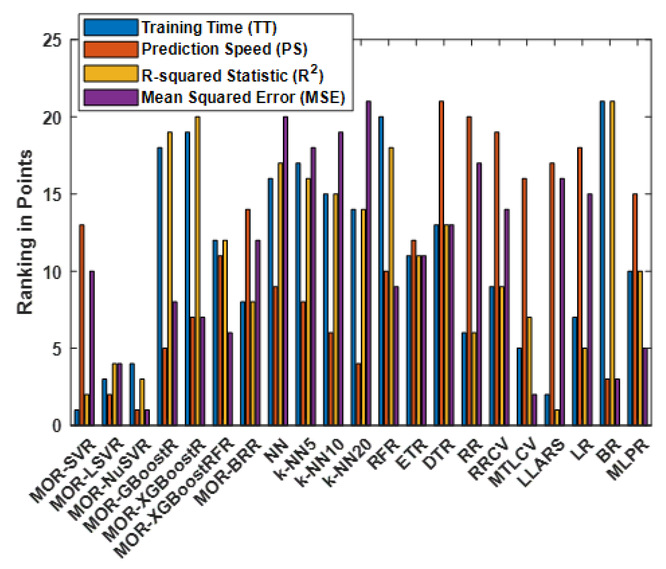
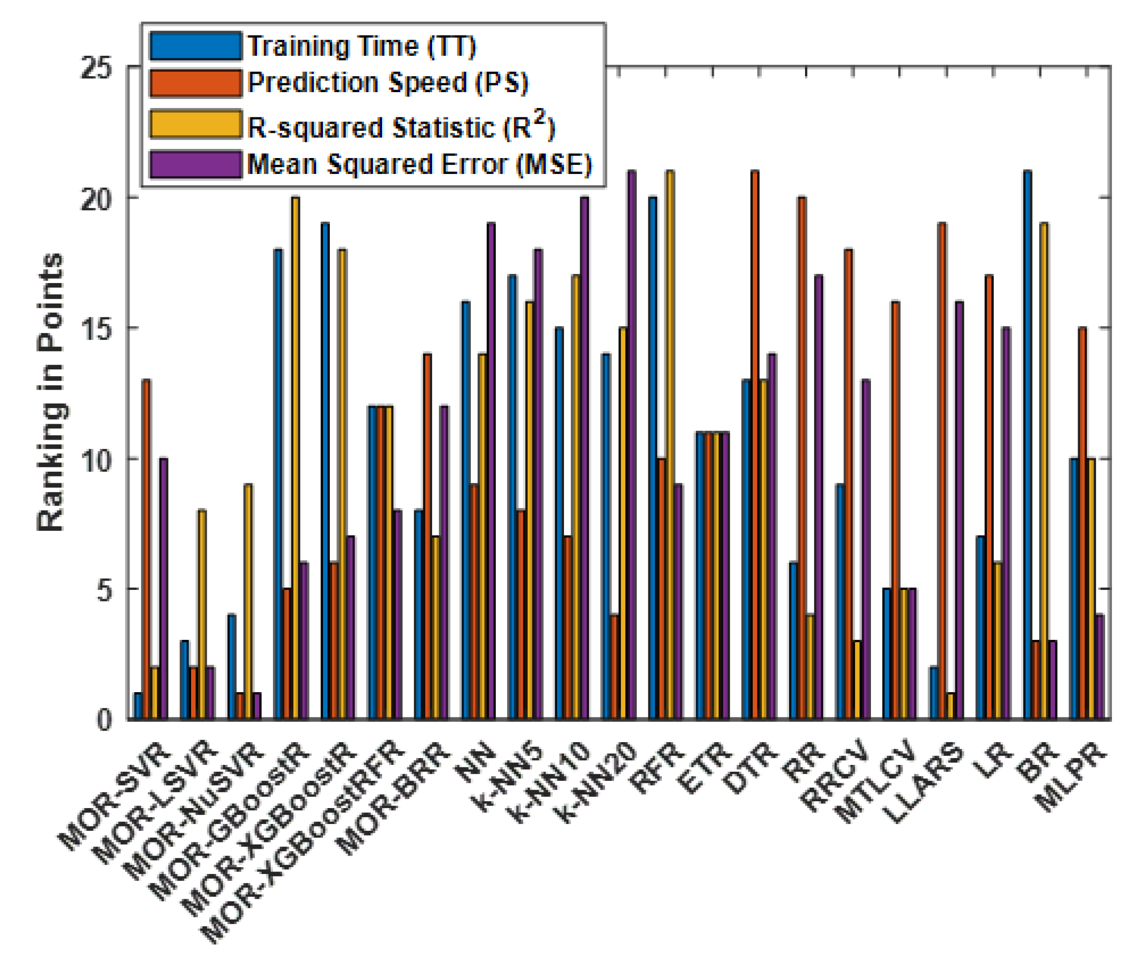
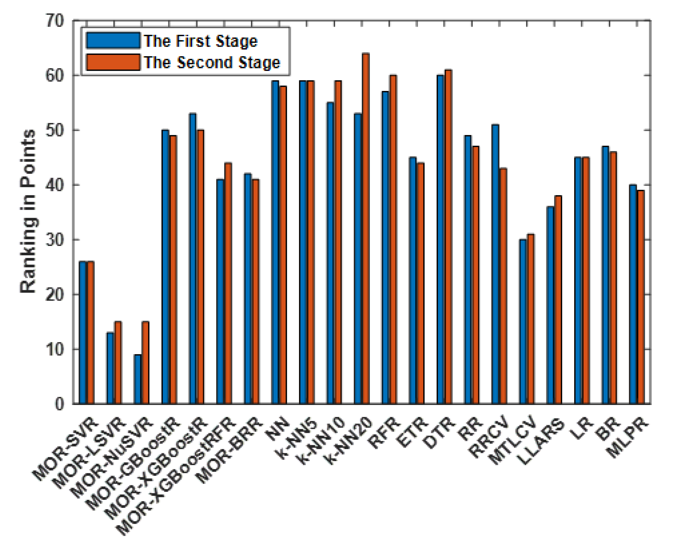
To straightforwardly rank all methods based on inference, positions or points are assigned to each method using their average performances (over the 50 independent statistical runs) for training time ( T T ), prediction speed ( P S ), R-squared values ( R 2 ) and mean squared error ( M S E ). The points are assigned in descending order of performance to have: 21, 20, 19, 18,…, 1. In this way, the best method(s) will have 21 points and the worst method(s) will have one point. Table 12 and Table 13 show how the overall points (sum of all points or the positions) obtained by each method can be used to deduce the overall ranking for the first and second stages of the predictive modeling of the multi-stage continuous-flow manufacturing process, respectively. These results are further corroborated in Figure 11, Figure 12 and Figure 13 where the ranking (in points) of all methods using the average values of their performance metrics (i.e., T T , P S , R 2 , and M S E ) over 50 statistical runs are shown for the first and second stages of the predictive modeling of the multi-stage continuous-flow manufacturing process.
For the first stage of the predictive modeling of the multi-stage continuous-flow manufacturing process, the overall rankings in Table 12 indicate that DTR ranks first with a total of 60 points, NN and k-NN5 both rank second with 59 points in total each. MOR-NuSVR ranks last with 9 points in total. This suggests that the overall performances of DTR, NN, and k-NN5 are better for the first stage of the predictive modeling of the multi-stage continuous-flow manufacturing process, in comparison to the other methods investigated. In a similar vein, for the second stage of the predictive modeling of the multi-stage continuous-flow manufacturing process, the overall rankings in Table 13 indicate that k-NN20 ranks first with a total of 64 points, DTR and RFR rank second and third, with 61 points in total, and 60 points in total, respectively. MOR-LSVR and MOR-NuSVR both rank last with 15 points in total each. This suggests that the overall performances of k-NN20, DTR, and RFR are better for the second stage of the predictive modeling of the multi-stage continuous-flow manufacturing process, in comparison to the other methods investigated. If the average number of points obtained by each method for the two stages of the predictive modeling of the multi-stage continuous-flow manufacturing process is used to select the overall best method, then DTR having an average of 60.5 points will be the overall best method for the predictive modeling of both stages of the multi-stage continuous-flow manufacturing process. To statistically verify that the overall performances of DTR and k-NN20 rank better than the other methods for the first and second stages of the predictive modeling of the multi-stage continuous-flow manufacturing process, respectively, hypothesis tests are carried out in the next subsection using the Wilcoxon test [59].

4.6. Hypothesis Test

A Wilcoxon test [59] is the hypothesis test used in this work to statistically verify the inference-based rankings detailed in Section 4.5. To carry out the test, the results obtained by all methods for training time ( T T ), predictive accuracy ( R 2 ), prediction speed ( P S ), and mean squared error ( M S E ) over the 50 independent statistical runs for each stage of the predictive modeling of the multi-stage continuous-flow manufacturing process are used as data samples. In this instance, the null hypothesis for the first stage of the predictive modeling of the multi-stage continuous-flow manufacturing process is that the data samples of DTR (the best method according to the inference-based ranking in Table 12) and the other methods have equal medians at 5% significance level (i.e., 95% confidence level). In a similar vein, the null hypothesis for the second stage of the predictive modeling of the multi-stage continuous-flow manufacturing process is that the data samples of k-NN20 (the best method according to the inference-based ranking in Table 13) and the other methods have equal medians at 5% significance level (i.e., 95% confidence level). For the two stages of the predictive modeling of the multi-stage continuous-flow manufacturing process, if the resultant probability value (p-value) of the hypothesis test is less than or equal to 0.05, then it can be said that a strong evidence exists against the null hypothesis and it is therefore rejected.
The results for the hypothesis tests are shown in Table 14 and Table 15, it can be said that T T , P S , R 2 , and M S E rejected the null hypothesis in all the cases according to the p-values reported in Table 14 and Table 15, except for NN and k-NN5 where the p-values for R 2 are greater than 0.05 for the second stage of the predictive modeling of the multi-stage continuous-flow manufacturing process. From the p-values reported in Table 14, it can be said that the T T , P S , R 2 , and M S E of DTR over the 50 independent runs are significantly better than the T T , P S , R 2 , and M S E of other methods for the first stage of the predictive modeling of the multi-stage continuous-flow manufacturing process. In a similar vein, the p-values reported in Table 15 also indicate that the T T , P S , and M S E of k-NN20 over the 50 independent runs are significantly better than the T T , P S , and M S E of other methods for the second stage of the predictive modeling. Also, from Table 15, it can be deduced that the R 2 of k-NN20 over the 50 independent runs are significantly better than the R 2 of all the other methods except for NN and k-NN5. These exceptions can be easily attributed to the stochastic nature and similarity of these methods and the number of statistical runs used for the experimentation. Therefore, the rankings earlier established in Table 12 and Table 13 can be said to be statistically valid.

5. Conclusions

A generalized framework for the predictive modeling of manufacturing processes via regression learning is presented and validated using an open-source data set for a multi-stage continuous-flow manufacturing process in this work. Specifically, the practicality of the framework is demonstrated by investigating several regression-based supervised learning techniques using the given data set. The investigated methods are appraised using the training time ( T T ), prediction speed ( P S ), predictive accuracy (R-squared statistic ( R 2 )), and mean squared error ( M S E ) obtained by each method over 50 independent statistical runs for the predictive modeling of the two stages of the multi-stage continuous-flow manufacturing process. The methods are then ranked inferentially according to the statistics of their metrics in terms of T T , P S , R 2 , and mean squared error ( M S E ) obtained by each method over the 50 independent statistical runs. Based on the inference-based rankings, DTR (decision tree regressor) and k-NN20 (k-nearest neighbour with 20 neighbors) have been identified as the most suitable regression learning techniques for the predictive modeling of the first stage and second stage of the multi-stage continuous-flow manufacturing process, respectively. These rankings are also verified statistically using a Wilcoxon rank sum test to validate the inferences drawn. Even though the experiments and outcomes in this work are not exhaustive due to the broad and stochastic nature of regression learning techniques, they can adequately serve as a guide and benchmark for the adoption and/or invention of regression learning-based paradigms in present-day and future manufacturing environments. In the future, a real-world paradigm where regression-based predictive models are employed on the fly in the manufacturing process will be investigated.

Author Contributions

Conceptualization, M.O.A.; methodology, M.O.A. and K.Z.; software, M.O.A. and K.Z.; validation M.O.A. and K.Z.; formal analysis, M.O.A.; investigation, M.O.A. and K.Z.; resources, M.O.A. and K.Z.; data curation, M.O.A. and K.Z.; writing—original draft preparation, M.O.A. and K.Z.; writing—review and editing, M.O.A.; visualization, M.O.A. and K.Z.; supervision, M.O.A.; project administration, M.O.A.; funding acquisition, M.O.A. All authors have read and agreed to the published version of the manuscript.

Funding

This research received no external funding. The APC for the publication of this work was fully supported by the editorial office.

Data Availability Statement

The open-source multi-flow continuous stage manufacturing data set used for the experiments in this paper is available at: https://www.kaggle.com/majidtabkhpaz, accessed on 18 October 2022.

Acknowledgments

The authors would like to especially thank the editorial office for the invitation to submit our manuscript and the APC waiver provided. The authors would also like to thank Liveline Technologies, U.S.A., for the availability of the open-source multi-stage continuous-flow manufacturing process data set.

Conflicts of Interest

The authors declare no conflict of interest.

References

  1. Bajic, B.; Rikalovic, A.; Suzic, N.; Piuri, V. Industry 4.0 Implementation Challenges and Opportunities: A Managerial Perspective. IEEE Syst. J. 2021, 15, 546–559. [Google Scholar] [CrossRef]
  2. Shiroishi, Y.; Uchiyama, K.; Suzuki, N. Society 5.0: For Human Security and Well-Being. Computer 2018, 51, 91–95. [Google Scholar] [CrossRef]
  3. Javaid, M.; Haleem, A. Critical components of Industry 5.0 towards a successful adoption in the field of manufacturing. J. Ind. Integr. Manag. 2020, 5, 327–348. [Google Scholar] [CrossRef]
  4. Malige, A.; Korcyl, G.; Firlej, M.; Fiutowski, T.; Idzik, M.; Korzeniak, B.; Lalik, R.; Misiak, A.; Molenda, A.; Moroń, J.; et al. Real-Time Data Processing Pipeline for Trigger Readout Board-Based Data Acquisition Systems. IEEE Trans. Nucl. Sci. 2022, 69, 1765–1772. [Google Scholar] [CrossRef]
  5. Akinsolu, M.O. Applied Artificial Intelligence in Manufacturing and Industrial Production Systems: PEST Considerations for Engineering Managers. IEEE Eng. Manag. Rev. 2022, 51, 1–8. [Google Scholar] [CrossRef]
  6. Miller, W.J.; Poole, M. Advanced CIM environment for manufacturing data analysis. IEEE Trans. Semicond. Manuf. 1993, 6, 128–133. [Google Scholar] [CrossRef]
  7. Zhang, H.; Wang, H.; Li, J.; Gao, H. A generic data analytics system for manufacturing production. Big Data Min. Anal. 2018, 1, 160–171. [Google Scholar] [CrossRef]
  8. Zhang, C.; Ji, W. Big Data Analysis Approach for Real-Time Carbon Efficiency Evaluation of Discrete Manufacturing Workshops. IEEE Access 2019, 7, 107730–107743. [Google Scholar] [CrossRef]
  9. Cui, Y.; Kara, S.; Chan, K.C. Manufacturing big data ecosystem: A systematic literature review. Robot.-Comput.-Integr. Manuf. 2020, 62, 101861. [Google Scholar] [CrossRef]
  10. Feng, M.; Li, Y. Predictive Maintenance Decision Making Based on Reinforcement Learning in Multistage Production Systems. IEEE Access 2022, 10, 18910–18921. [Google Scholar] [CrossRef]
  11. Costello, J.J.A.; West, G.M.; McArthur, S.D.J. Machine Learning Model for Event-Based Prognostics in Gas Circulator Condition Monitoring. IEEE Trans. Reliab. 2017, 66, 1048–1057. [Google Scholar] [CrossRef] [Green Version]
  12. Ayodeji, A.; Wang, Z.; Wang, W.; Qin, W.; Yang, C.; Xu, S.; Liu, X. Causal augmented ConvNet: A temporal memory dilated convolution model for long-sequence time series prediction. ISA Trans. 2022, 123, 200–217. [Google Scholar] [CrossRef] [PubMed]
  13. Boyes, H.; Hallaq, B.; Cunningham, J.; Watson, T. The industrial internet of things (IIoT): An analysis framework. Comput. Ind. 2018, 101, 1–12. [Google Scholar] [CrossRef]
  14. Aebersold, S.A.; Akinsolu, M.O.; Monir, S.; Jones, M.L. Ubiquitous Control of a CNC Machine: Proof of Concept for Industrial IoT Applications. Information 2021, 12, 529. [Google Scholar] [CrossRef]
  15. Siva Vardhan, D.S.V.; Narayan, Y.S. Development of an automatic monitoring and control system for the objects on the conveyor belt. In Proceedings of the 2015 International Conference on Man and Machine Interfacing (MAMI), Bhubaneswar, India, 17–19 December 2015; pp. 1–6. [Google Scholar] [CrossRef]
  16. Çınar, Z.M.; Abdussalam Nuhu, A.; Zeeshan, Q.; Korhan, O.; Asmael, M.; Safaei, B. Machine learning in predictive maintenance towards sustainable smart manufacturing in industry 4.0. Sustainability 2020, 12, 8211. [Google Scholar] [CrossRef]
  17. Djurdjanovic, D.; Lee, J.; Ni, J. Watchdog Agent—An infotronics-based prognostics approach for product performance degradation assessment and prediction. Adv. Eng. Inform. 2003, 17, 109–125. [Google Scholar] [CrossRef]
  18. Liu, C.; Tang, D.; Zhu, H.; Nie, Q. A Novel Predictive Maintenance Method Based on Deep Adversarial Learning in the Intelligent Manufacturing System. IEEE Access 2021, 9, 49557–49575. [Google Scholar] [CrossRef]
  19. Liu, H.; Yuan, R.; Lv, Y.; Li, H.; Gedikli, E.D.; Song, G. Remaining Useful Life Prediction of Rolling Bearings Based on Segmented Relative Phase Space Warping and Particle Filter. IEEE Trans. Instrum. Meas. 2022, 71, 1–15. [Google Scholar] [CrossRef]
  20. He, J.; Cen, Y.; Alelaumi, S.; Won, D. An Artificial Intelligence-Based Pick-and-Place Process Control for Quality Enhancement in Surface Mount Technology. IEEE Trans. Components Packag. Manuf. Technol. 2022, 12, 1702–1711. [Google Scholar] [CrossRef]
  21. Dogan, A.; Birant, D. Machine learning and data mining in manufacturing. Expert Syst. Appl. 2021, 166, 114060. [Google Scholar] [CrossRef]
  22. Cui, P.H.; Wang, J.Q.; Li, Y. Data-driven modelling, analysis and improvement of multistage production systems with predictive maintenance and product quality. Int. J. Prod. Res. 2021, 60, 1–18. [Google Scholar] [CrossRef]
  23. Liveline Technologies. Multi-Stage Continuous-Flow Manufacturing Process. 2019. Available online: https://www.kaggle.com/datasets/supergus/multistage-continuousflow-manufacturing-process (accessed on 15 October 2022).
  24. Liveline Technologies. Convert Your Manufacturing Assets into an Intelligent, Autonomous System Using AI-Based Process Controls. 2022. Available online: https://www.liveline.tech/ (accessed on 5 December 2022).
  25. Pach, F.; Feil, B.; Nemeth, S.; Arva, P.; Abonyi, J. Process-data-warehousing-based operator support system for complex production technologies. IEEE Trans. Syst. Man Cybern.- Part A Syst. Hum. 2006, 36, 136–153. [Google Scholar] [CrossRef]
  26. LJ Create. PETRA II Advanced Industrial Control Trainer. 2023. Available online: https://ljcreate.com/uk/engineering/petra-ii-advanced-industrial-control-trainer/ (accessed on 7 January 2023).
  27. Nargesian, F.; Samulowitz, H.; Khurana, U.; Khalil, E.B.; Turaga, D.S. Learning Feature Engineering for Classification. In Proceedings of the Twenty-Sixth International Joint Conference on Artificial Intelligence (IJCAI-17), Melbourne, Australia, 19–25 August 2017; pp. 2529–2535. [Google Scholar]
  28. Wan, X. Influence of feature scaling on convergence of gradient iterative algorithm. J. Phys. Conf. Ser. 2019, 1213, 032021. [Google Scholar] [CrossRef] [Green Version]
  29. Sangodoyin, A.O.; Akinsolu, M.O.; Pillai, P.; Grout, V. Detection and Classification of DDoS Flooding Attacks on Software-Defined Networks: A Case Study for the Application of Machine Learning. IEEE Access 2021, 9, 122495–122508. [Google Scholar] [CrossRef]
  30. Akinsolu, M.O.; Sangodoyin, A.O.; Uyoata, U.E. Behavioral Study of Software-Defined Network Parameters Using Exploratory Data Analysis and Regression-Based Sensitivity Analysis. Mathematics 2022, 10, 2536. [Google Scholar] [CrossRef]
  31. Sangodoyin, A.O.; Akinsolu, M.O.; Awan, I. A deductive approach for the sensitivity analysis of software defined network parameters. Simul. Model. Pract. Theory 2020, 103, 102099. [Google Scholar] [CrossRef]
  32. Liu, P.; Lv, N.; Chen, K.; Tang, L.; Zhou, J. Regression Based Dynamic Elephant Flow Detection in Airborne Network. IEEE Access 2020, 8, 217123–217133. [Google Scholar] [CrossRef]
  33. Shohani, R.B.; Mostafavi, S.A. Introducing a New Linear Regression Based Method for Early DDoS Attack Detection in SDN. In Proceedings of the 2020 6th International Conference on Web Research (ICWR), Tehran, Iran, 22–23 April 2020; pp. 126–132. [Google Scholar] [CrossRef]
  34. Borchani, H.; Varando, G.; Bielza, C.; Larranaga, P. A survey on multi-output regression. Wiley Interdiscip. Rev. Data Min. Knowl. Discov. 2015, 5, 216–233. [Google Scholar] [CrossRef]
  35. Montesinos López, O.A.; Montesinos López, A.; Crossa, J. Support Vector Machines and Support Vector Regression. In Multivariate Statistical Machine Learning Methods for Genomic Prediction; Springer: Cham, Switzerland, 2022; pp. 337–378. [Google Scholar]
  36. scikit-learn. scikit-learn Machine Learning in Python. 2022. Available online: https://scikit-learn.org/stable/ (accessed on 15 October 2022).
  37. Platt, J. Probabilistic outputs for support vector machines and comparisons to regularized likelihood methods. Adv. Large Margin Classif. 1999, 10, 61–74. [Google Scholar]
  38. Friedman, J.H. Stochastic gradient boosting. Comput. Stat. Data Anal. 2002, 38, 367–378. [Google Scholar] [CrossRef]
  39. Friedman, J.H. Greedy function approximation: A gradient boosting machine. Ann. Stat. 2001, 29, 1189–1232. [Google Scholar] [CrossRef]
  40. Breiman, L. Random forests. Mach. Learn. 2001, 45, 5–32. [Google Scholar] [CrossRef] [Green Version]
  41. Tipping, M.E. Sparse Bayesian learning and the relevance vector machine. J. Mach. Learn. Res. 2001, 1, 211–244. [Google Scholar]
  42. Dudani, S.A. The Distance-Weighted k-Nearest-Neighbor Rule. IEEE Trans. Syst. Man Cybern. 1976, SMC-6, 325–327. [Google Scholar] [CrossRef]
  43. An efficient instance selection algorithm for k nearest neighbor regression. Neurocomputing 2017, 251, 26–34. [CrossRef]
  44. Ho, T.K. Random decision forests. In Proceedings of the 3rd International Conference on Document Analysis and Recognition, Montreal, QC, Canada, 14–16 August 1995; Volume 1, pp. 278–282. [Google Scholar]
  45. Xu, M.; Watanachaturaporn, P.; Varshney, P.K.; Arora, M.K. Decision tree regression for soft classification of remote sensing data. Remote Sens. Environ. 2005, 97, 322–336. [Google Scholar] [CrossRef]
  46. Geurts, P.; Ernst, D.; Wehenkel, L. Extremely randomized trees. Mach. Learn. 2006, 63, 3–42. [Google Scholar] [CrossRef] [Green Version]
  47. McDonald, G.C. Ridge regression. Wiley Interdiscip. Rev. Comput. Stat. 2009, 1, 93–100. [Google Scholar] [CrossRef]
  48. Nokeri, T.C. Advanced Parametric Methods. In Data Science Revealed; Apress: Berkley, CA, USA, 2021; pp. 45–53. [Google Scholar]
  49. Liu, K.; Xu, B.; Kim, C.; Fu, J. Well performance from numerical methods to machine learning approach: Applications in multiple fractured shale reservoirs. Geofluids 2021, 2021, 3169456. [Google Scholar] [CrossRef]
  50. Hesterberg, T.; Choi, N.H.; Meier, L.; Fraley, C. Least angle and 1 penalized regression: A review. Stat. Surv. 2008, 2, 61–93. [Google Scholar] [CrossRef]
  51. Cohen, P.; West, S.G.; Aiken, L.S. Applied Multiple Regression/Correlation Analysis for the Behavioral Sciences; Lawrence Erlbaum Associates, Inc.: Mahwah, NJ, USA, 2003. [Google Scholar]
  52. Breiman, L. Bagging predictors. Mach. Learn. 1996, 24, 123–140. [Google Scholar] [CrossRef] [Green Version]
  53. Negnevitsky, M. Artificial Intelligence: A Guide to Intelligent Systems; Pearson Education: Harlow, UK, 2005. [Google Scholar]
  54. Pedregosa, F.; Varoquaux, G.; Gramfort, A.; Michel, V.; Thirion, B.; Grisel, O.; Blondel, M.; Prettenhofer, P.; Weiss, R.; Dubourg, V.; et al. Scikit-learn: Machine learning in Python. J. Mach. Learn. Res. 2011, 12, 2825–2830. [Google Scholar]
  55. Google Research. Colaboratory. 2022. Available online: https://colab.research.google.com/ (accessed on 15 October 2022).
  56. Isabona, J.; Imoize, A.L.; Kim, Y. Machine Learning-Based Boosted Regression Ensemble Combined with Hyperparameter Tuning for Optimal Adaptive Learning. Sensors 2022, 22, 3776. [Google Scholar] [CrossRef] [PubMed]
  57. Passos, D.; Mishra, P. A tutorial on automatic hyperparameter tuning of deep spectral modelling for regression and classification tasks. Chemom. Intell. Lab. Syst. 2022, 223, 104520. [Google Scholar] [CrossRef]
  58. Chicco, D. Ten quick tips for machine learning in computational biology. BioData Min. 2017, 10, 1–17. [Google Scholar] [CrossRef]
  59. Wilcoxon, F. Individual comparisons by ranking methods. In Breakthroughs in Statistics; Springer: New York, NY, USA, 1992; pp. 196–202. [Google Scholar]
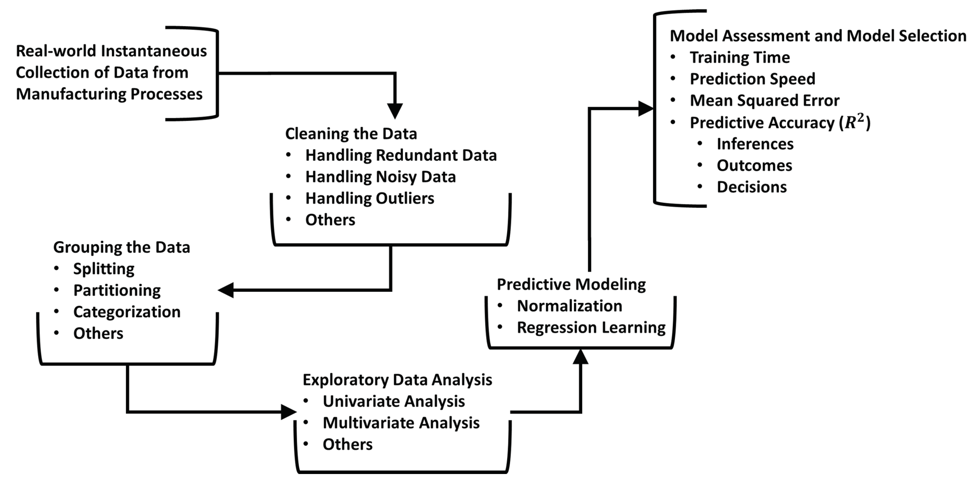
Figure 1. The proposed generalized framework.
Inventions 08 00032 g001
Figure 2. Architecture of the manufacturing process used as a case study.
Inventions 08 00032 g002
Figure 3. Box plots of T T (over 50 statistical runs) for all methods for the first stage.
Inventions 08 00032 g003
Figure 4. Box plots of T T (over 50 statistical runs) for all methods for the second stage.
Inventions 08 00032 g004
Figure 5. Box plots of P S (over 50 statistical runs) for all methods for the first stage.
Inventions 08 00032 g005
Figure 6. Box plots of P S (over 50 statistical runs) for all methods for the second stage.
Inventions 08 00032 g006
Figure 7. Box plots of R 2 statistic (over 50 statistical runs) for all methods for the first stage.
Inventions 08 00032 g007
Figure 8. Box plots of R 2 statistic (over 50 statistical runs) for all methods for the second stage.
Inventions 08 00032 g008
Figure 9. Box plots of M S E (over 50 statistical runs) for all methods for the first stage.
Inventions 08 00032 g009
Figure 10. Box plots of M S E (over 50 statistical runs) for all methods for the second stage.
Inventions 08 00032 g010
Figure 11. Ranking (in points) of all methods using the average values of their performance metrics (i.e., T T , P S , R 2 , and M S E ) over 50 statistical runs for the first stage.
Inventions 08 00032 g011
Figure 12. Ranking (in points) of all methods using the average values of their performance metrics (i.e., T T , P S , R 2 , and M S E ) over 50 statistical runs for the second stage.
Inventions 08 00032 g012
Figure 13. Overall ranking (in points) of all methods using the average values of their performance metrics (i.e., T T , P S , R 2 , and M S E ) over 50 statistical runs.
Inventions 08 00032 g013
Table 1. Descriptive statistics of the explanatory variables (non-normalized) from the data set.
Explanatory VariableMeanMedianMinimumMaximumS.D.
First Condition: F A C 1 15.315.113.817.21.2
Second Condition: F A C 2 23.823.923.024.40.4
First Stage: M 1 P V 1 1242.81264.4231.31331.895.8
First Stage: M 1 P V 2 72.072.071.972.50.1
First Stage: M 1 P V 3 72.072.071.372.70.4
First Stage: M 1 P V 4 70.372.044.488.55.5
First Stage: M 1 P V 5 11.110.710.412.20.6
First Stage: M 1 P V 6 409.0417.0359.5487.220.5
First Stage: M 1 P V 7 81.581.376.383.90.9
First Stage: M 1 P V 8 76.075.069.780.02.1
First Stage: M 2 P V 1 202.6203.30.0266.515.1
First Stage: M 2 P V 2 69.069.068.769.70.1
First Stage: M 2 P V 3 69.169.167.869.90.1
First Stage: M 2 P V 4 73.473.471.674.40.4
First Stage: M 2 P V 5 13.913.913.814.00.0
First Stage: M 2 P V 6 226.1226.1218.9250.63.1
First Stage: M 2 P V 7 76.877.068.877.40.9
First Stage: M 2 P V 8 60.060.059.660.50.2
First Stage: M 3 P V 1 202.4202.90.0259.115.7
First Stage: M 3 P V 2 78.078.077.378.70.1
First Stage: M 3 P V 3 78.078.077.778.60.1
First Stage: M 3 P V 4 345.1342.9321.2374.39.1
First Stage: M 3 P V 5 13.313.412.014.00.4
First Stage: M 3 P V 6 246.8247.5235.1263.76.1
First Stage: M 3 P V 7 74.175.165.375.52.1
First Stage: M 3 P V 8 65.065.064.865.20.1
First Stage: T C O M B 1 108.9105.545.3118.95.7
First Stage: T C O M B 2 84.974.853.3115.218.6
First Stage: T C O M B 3 80.080.079.680.30.1
Second Stage: M 4 P V 1 360.1360.0298.0393.02.3
Second Stage: M 4 P V 2 360.1360.0284.0396.03.0
Second Stage: M 4 P V 3 17.217.014.025.00.9
Second Stage: M 4 P V 4 322.6324.0268.0327.03.7
Second Stage: M 4 P V 5 17.217.014.025.00.9
Second Stage: M 4 P V 6 309.8311.0260.0326.02.9
Second Stage: M 4 P V 7 187.1192.035.0216.023.7
Second Stage: M 5 P V 1 310.0310.0309.4310.30.0
Second Stage: M 5 P V 2 290.0290.0289.7290.30.1
Second Stage: M 5 P V 3 269.7270.0263.8270.01.0
Second Stage: M 5 P V 4 242.7242.7237.6245.01.6
Second Stage: M 5 P V 5 245.0245.0242.9245.70.1
Second Stage: M 5 P V 6 63.463.462.866.10.4
Second Stage: M 5 P V 7 154.0155.645.4159.210.3
Table 2. Descriptive statistics of the response variables (non-normalized) from the data set.
Response VariableMeanMedianMinimumMaximumS.D.
First Stage: S 1 C O 1 12.913.00.020.90.9
First Stage: S 1 C O 2 8.113.2−3.119.16.9
First Stage: S 1 C O 3 11.411.3−4.923.51.1
First Stage: S 1 C O 4 21.321.50.026.22.1
First Stage: S 1 C O 5 32.933.5−7.734.83.9
First Stage: S 1 C O 6 0.10.0−0.65.00.6
First Stage: S 1 C O 7 1.31.6−0.87.01.1
First Stage: S 1 C O 8 1.10.0−0.85.21.4
First Stage: S 1 C O 9 19.820.9 6.6 × 10 10 22.54.8
First Stage: S 1 C O 10 18.018.9 3.6 × 10 3 20.44.2
First Stage: S 1 C O 11 7.77.8 1.4 × 10 3 13.11.1
First Stage: S 1 C O 12 1.50.0 1.6 × 10 20 7.52.5
First Stage: S 1 C O 13 1.21.5 3.5 × 10 4 4.00.7
First Stage: S 1 C O 14 2.93.2−1.26.90.9
First Stage: S 1 C O 15 9.915.0−6.622.37.4
Second Stage: S 2 C O 1 11.712.8 9.8 × 10 137 19.13.6
Second Stage: S 2 C O 2 6.36.5 3.0 × 10 5 12.91.6
Second Stage: S 2 C O 3 10.310.9 3.3 × 10 107 16.52.3
Second Stage: S 2 C O 4 19.320.6 6.6 × 10 107 25.24.7
Second Stage: S 2 C O 5 2.90.0 1.4 × 10 13 34.39.2
Second Stage: S 2 C O 6 2.72.7 3.5 × 10 95 8.10.4
Second Stage: S 2 C O 7 0.50.6 3.7 × 10 105 3.30.2
Second Stage: S 2 C O 8 2.93.0 1.3 × 10 109 7.40.5
Second Stage: S 2 C O 9 18.419.7 3.0 × 10 104 24.85.0
Second Stage: S 2 C O 10 11.616.6 3.7 × 10 3 18.47.6
Second Stage: S 2 C O 11 7.57.9 5.2 × 10 95 8.61.6
Second Stage: S 2 C O 12 5.45.6 2.7 × 10 95 6.31.2
Second Stage: S 2 C O 13 2.02.1 6.2 × 10 96 5.20.4
Second Stage: S 2 C O 14 3.53.5 1.8 × 10 95 8.00.5
Second Stage: S 2 C O 15 7.57.9−3.414.32.1
Table 3. The regression learning methods investigated.
MethodReferences
MOR-based Support Vector Regression (MOR-SVR)[34,35,36]
MOR-based Linear Support Vector Regression (MOR-LSVR)[34,35,36]
MOR-based N u Support Vector Regression (MOR-NuSVR)[34,36,37]
MOR-based Gradient Boosting Regression (MOR-GBoostR)[34,36,38]
MOR-based Extreme Gradient Boosting Regression (MOR-XGBoostR)[34,36,38,39]
MOR-based Extreme Gradient Boosting Random Forest
Regression (MOR-XGBoostRFR)
[34,36,40]
MOR-based Bayesian Ridge Regression (MOR-BRR)[34,36,41]
k-Nearest Neighbors (k-NN)[36,42,43]
Random Forest Regressor (RFR)[36,40,44]
Decision Trees Regressor (DTR)[36,45]
Extra-Trees Regressor (ETR)[36,46]
Ridge Regression (RR)[36,47]
Ridge Regression with Built-In Cross-Validation (RRCV)[36,48]
Multi-Task Least Absolute Shrinkage and Selection Operator
with Cross-Validation (MTLCV)
[36,49]
Least Absolute Shrinkage and Selection Operator Model Fit
Least Angle Regression (LLARS)
[36,50]
Linear Regression (LR)[36,51]
Bagging Regressor (BR)[36,52]
Multilayer Perceptron Regressor (MLPR)[36,53]
Table 4. Training time (in milliseconds (ms)) for all methods over 50 statistical runs (the first stage).
MethodBestWorstAverageMedianS.D.
MOR-SVR4575.96671.04827.94727.1400.7
MOR-LSVR40,305.448,648.842,700.942,682.01434.7
MOR-NuSVR113,936.0123,388.0117,689.1117,561.51963.4
MOR-GBoostR11,168.314,176.813,158.513,318.5673.0
MOR-XGBoostR13,315.416,089.913,712.113,588.3533.6
MOR-XGBoostRFR14,293.315,382.814,749.814,687.6239.4
MOR-BRR319.4344.6331.8331.35.5
NN1.86.34.95.00.5
k-NN53.55.85.15.20.4
k-NN103.85.45.05.10.3
k-NN203.65.44.84.90.4
RFR7006.47704.17206.67170.0158.5
ETR1200.71245.81213.41211.58.5
DTR57.471.660.258.63.6
RR5.57.75.95.80.4
RRCV37.255.144.243.73.5
MTLCV56,858.465,233.860,883.660,837.82035.8
LLARS13.361.715.914.37.1
LR22.933.326.826.42.4
BR57,496.661,163.258,489.658,287.5806.4
MLPR21,222.525,145.922,101.622,172.1571.8
Table 5. Training time (in milliseconds (ms)) for all methods over 50 statistical runs (the second stage).
MethodBestWorstAverageMedianS.D.
MOR-SVR2255.42489.42288.42281.933.8
MOR-LSVR37,700.341,578.939,647.939,768.1983.8
MOR-NuSVR87,112.392,142.790,015.089,941.3967.9
MOR-GBoostR6050.47306.26888.96994.2364.5
MOR-XGBoostR6132.97488.96348.66313.3191.8
MOR-XGBoostRFR5589.77371.55808.35720.9297.4
MOR-BRR180.9201.1186.4185.54.0
NN1.65.64.54.50.5
k-NN53.74.84.54.50.2
k-NN103.54.74.44.40.2
k-NN203.14.84.24.30.4
RFR2258.42584.22308.92282.472.5
ETR740.5845.3756.7752.016.3
DTR19.622.620.220.00.6
RR4.56.24.84.70.3
RRCV25.632.328.027.51.6
MTLCV17,352.719,314.418,337.518,385.4384.9
LLARS9.913.711.311.10.8
LR13.820.916.315.91.7
BR33,483.836,263.534,183.634,043.4495.9
MLPR19,726.420,654.020,127.920,117.5220.0
Table 6. Prediction speed (in observations per second (obs/s)) for all methods over 50 statistical runs (first stage).
MethodBestWorstAverageMedianS.D.
MOR-SVR 5.6239 × 10 5 4.1334 × 10 5 4.9186 × 10 5 4.8717 × 10 5 2.9146 × 10 4
MOR-LSVR 1.5552 × 10 2 1.2501 × 10 2 1.4115 × 10 2 1.4085 × 10 2 5.9448
MOR-NuSVR 9.6049 × 10 1 8.5853 × 10 1 9.2834 × 10 1 9.2775 × 10 1 2.1876
MOR-GBRoostR 3.4622 × 10 4 2.2161 × 10 4 3.0139 × 10 4 3.0336 × 10 4 2.1214 × 10 3
MOR-XGBoostR 3.5163 × 10 4 2.4821 × 10 4 3.3007 × 10 4 3.3504 × 10 4 1.9354 × 10 3
MOR-XGBoostRFR 1.0518 × 10 5 7.5331 × 10 4 1.0015 × 10 5 1.0069 × 10 5 4.3709 × 10 3
MOR-BRR 5.6375 × 10 5 4.8359 × 10 5 5.1224 × 10 5 5.1097 × 10 5 1.4630 × 10 4
NN 4.2699 × 10 4 2.2612 × 10 4 3.8062 × 10 4 3.8004 × 10 4 3.2043 × 10 3
k-NN5 4.1211 × 10 4 2.6105 × 10 4 3.7383 × 10 4 3.7048 × 10 4 2.8666 × 10 3
k-NN10 3.7018 × 10 4 2.0611 × 10 4 3.2667 × 10 4 3.2526 × 10 4 3.1338 × 10 3
k-NN20 2.9755 × 10 4 2.3212 × 10 4 2.7355 × 10 4 2.7384 × 10 4 1.4434 × 10 3
RFR 8.7096 × 10 4 7.5532 × 10 4 8.4908 × 10 4 8.5385 × 10 4 1.9828 × 10 3
ETR 1.1799 × 10 5 1.0883 × 10 5 1.1583 × 10 5 1.1622 × 10 5 1.5385 × 10 3
DTR 5.2917 × 10 6 3.8139 × 10 6 4.8691 × 10 6 4.9929 × 10 6 3.2706 × 10 5
RR 4.6171 × 10 6 2.5956 × 10 6 4.0102 × 10 6 4.1101 × 10 6 3.9870 × 10 5
RRCV 4.1563 × 10 6 2.3477 × 10 6 3.8520 × 10 6 3.9050 × 10 6 2.9426 × 10 5
MTLCV 3.7941 × 10 6 2.4586 × 10 6 3.4746 × 10 6 3.4643 × 10 6 2.3376 × 10 5
LLARS 4.1514 × 10 6 1.4018 × 10 6 3.6085 × 10 6 3.7444 × 10 6 5.4622 × 10 5
LR 4.1822 × 10 6 2.4105 × 10 6 3.6997 × 10 6 3.7071 × 10 6 3.1664 × 10 5
BR 3.5379 × 10 3 2.9929 × 10 3 3.4633 × 10 3 3.4946 × 10 3 1.0798 × 10 2
MLPR 1.0661 × 10 6 2.2993 × 10 5 8.9940 × 10 5 9.4811 × 10 5 1.6888 × 10 5
Table 7. Prediction speed (in observations per second (obs/s)) for all methods over 50 statistical runs (second stage).
MethodBestWorstAverageMedianS.D.
MOR-SVR 4.5950 × 10 5 3.5034 × 10 5 4.1594 × 10 5 4.2574 × 10 5 2.2816 × 10 4
MOR-LSVR 1.9021 × 10 2 1.6441 × 10 2 1.7654 × 10 2 1.7680 × 10 2 5.6600
MOR-NuSVR 1.3475 × 10 2 1.2274 × 10 2 1.3128 × 10 2 1.3213 × 10 2 2.7050
MOR-GBoostR 3.9727 × 10 4 2.8796 × 10 4 3.4560 × 10 4 3.4269 × 10 4 2.2557 × 10 3
MOR-XGBoostR 3.8692 × 10 4 2.8567 × 10 4 3.6527 × 10 4 3.6795 × 10 4 1.7434 × 10 3
MOR-XGBoostRFR 1.2194 × 10 5 7.9684 × 10 4 1.1630 × 10 5 1.1776 × 10 5 6.0654 × 10 3
MOR-BRR 6.6072 × 10 5 4.5947 × 10 5 5.7582 × 10 5 5.7859 × 10 5 3.3941 × 10 4
NN 5.1418 × 10 4 4.0254 × 10 4 4.6993 × 10 4 4.7415 × 10 4 2.0383 × 10 3
k-NN5 4.9592 × 10 4 4.0310 × 10 4 4.5902 × 10 4 4.6354 × 10 4 2.0259 × 10 3
k-NN10 4.3716 × 10 4 3.6807 × 10 4 4.0243 × 10 4 3.9825 × 10 4 1.9493 × 10 3
k-NN20 3.4977 × 10 4 2.5228 × 10 4 3.1848 × 10 4 3.1948 × 10 4 1.8785 × 10 3
RFR 8.6406 × 10 4 7.6123 × 10 4 8.4357 × 10 4 8.5108 × 10 4 2.2585 × 10 3
ETR 1.1598 × 10 5 1.0321 × 10 5 1.1374 × 10 5 1.1470 × 10 5 2.7651 × 10 3
DTR 6.0917 × 10 6 4.0165 × 10 6 5.6784 × 10 6 5.8007 × 10 6 4.2400 × 10 5
RR 4.7774 × 10 6 3.2762 × 10 6 4.4236 × 10 6 4.4792 × 10 6 2.2114 × 10 5
RRCV 4.3636 × 10 6 3.3754 × 10 6 4.0458 × 10 6 4.0721 × 10 6 1.9418 × 10 5
MTLCV 3.7229 × 10 6 2.4182 × 10 6 3.3676 × 10 6 3.5491 × 10 6 3.8213 × 10 5
LLARS 4.6237 × 10 6 2.1289 × 10 6 4.1231 × 10 6 4.2340 × 10 6 4.4958 × 10 5
LR 4.3447 × 10 6 2.8044 × 10 6 3.9983 × 10 6 4.0774 × 10 6 3.2755 × 10 5
BR 3.6302 × 10 3 3.3082 × 10 3 3.5747 × 10 3 3.5933 × 10 3 6.4570 × 10 1
MLPR 1.0929 × 10 6 2.4127 × 10 5 1.0069 × 10 6 1.0317 × 10 6 1.2004 × 10 5
Table 8. R-squared value ( R 2 ) for all methods over 50 statistical runs (first stage).
MethodBestWorstAverageMedianS.D.
MOR-SVR0.1990.1760.1880.1880.005
MOR-LSVR0.3050.2830.2950.2950.005
MOR-NuSVR0.2960.2760.2860.2860.004
MOR-GBoostR0.6880.6390.6630.6640.011
MOR-XGBoostR0.7010.6330.6730.6760.016
MOR-XGBoostRFR0.4430.4140.4280.4270.006
MOR-BRR0.3270.3030.3170.3170.004
NN0.6280.5640.5940.5960.016
k-NN50.6220.5540.5920.5910.013
k-NN100.5940.5330.5700.5720.015
k-NN200.5350.5050.5230.5240.007
RFR0.6930.6200.6610.6600.015
ETR0.3970.3660.3800.3790.006
DTR0.4500.3380.4360.4380.015
RR0.3270.3090.3170.3170.003
RRCV0.3260.3100.3170.3170.004
MTLCV0.3250.3090.3170.3170.003
LLARS0.1890.1800.1850.1850.002
LR0.3230.3080.3170.3160.003
BR0.7470.6980.7280.7280.010
MLPR0.4040.3570.3760.3750.009
Table 9. R-squared value ( R 2 ) for all methods over 50 statistical runs (second stage).
MethodBestWorstAverageMedianS.D.
MOR-SVR0.4940.4340.4630.4630.015
MOR-LSVR0.5740.5000.5440.5440.015
MOR-NuSVR0.5800.5190.5490.550.013
MOR-GBoostR0.7650.6910.7360.7350.013
MOR-XGBoostR0.7480.6940.7260.7260.013
MOR-XGBoostRFR0.6790.6250.6570.6570.012
MOR-BRR0.5680.5170.5440.5460.012
NN0.7330.6860.7060.7030.012
k-NN50.7290.6940.7090.7100.009
k-NN100.7390.6860.7130.7150.013
k-NN200.7250.6870.7080.7080.010
RFR0.7690.7260.7460.7460.010
ETR0.6750.6040.6480.6490.014
DTR0.6890.6350.6620.6600.012
RR0.5680.5110.5400.5410.015
RRCV0.5640.4970.5380.5390.014
MTLCV0.5730.5110.5410.5430.013
LLARS0.2860.2600.2750.2760.005
LR0.5690.5160.5420.5430.012
BR0.7480.7090.7300.7300.010
MLPR0.6210.5570.5920.5920.014
Table 10. Mean squared error (MSE) for all methods over 50 statistical runs (the first stage).
MethodBestWorstAverageMedianS.D.
MOR-SVR8.49.99.09.00.3
MOR-LSVR7.48.88.18.10.3
MOR-NuSVR7.48.78.18.10.3
MOR-GBoostR3.13.63.43.40.1
MOR-XGBoostR3.03.53.23.30.1
MOR-XGBoostRFR5.16.05.65.60.2
MOR-BRR6.77.47.07.10.2
NN3.74.44.14.10.2
k-NN53.84.34.14.00.1
k-NN103.94.64.24.20.1
k-NN204.35.14.74.60.2
RFR2.83.43.13.10.1
ETR5.56.45.95.90.2
DTR4.46.04.94.90.2
RR6.57.47.07.00.2
RRCV6.57.67.07.00.2
MTLCV6.67.47.07.00.2
LLARS7.88.98.38.30.2
LR6.47.77.07.00.2
BR2.53.12.72.70.1
MLPR5.56.55.95.90.2
Table 11. Mean squared error (MSE) for all methods over 50 statistical runs (the second stage).
MethodBestWorstAverageMedianS.D.
MOR-SVR10.311.610.910.90.3
MOR-LSVR9.610.810.210.20.3
MOR-NuSVR9.510.910.310.30.3
MOR-GBoostR3.33.93.63.70.1
MOR-XGBoostR3.44.03.73.70.1
MOR-XGBoostRFR5.76.36.06.00.1
MOR-BR8.09.18.58.50.2
NN3.74.34.14.10.1
k-NN53.94.44.14.00.1
k-NN103.84.34.14.00.1
k-NN204.04.64.34.30.1
RFR3.23.83.53.50.1
ETR5.66.46.06.00.2
DTR5.05.75.35.30.2
RR8.08.98.58.50.2
RRCV8.09.08.58.50.2
MTLCV8.19.08.58.50.2
LLARS8.69.89.29.20.2
LR8.18.98.58.50.2
BR3.23.83.53.50.1
MLPR6.87.97.37.30.2
Table 12. Ranking (in points) of all methods (the first stage).
Method TT PS R 2 MSE Overall
MOR-SVR11321026
MOR-LSVR324413
MOR-NuSVR41319
MOR-GBoostR18519850
MOR-XGBoostR19720753
MOR-GBoostRFR121112641
MOR-BR81481242
NN169172059
k-NN5178161859
k-NN10156151955
k-NN20144142153
RFR201018957
ETR1112111145
DTR1321131360
RR62061749
RRCV91991451
MTLCV5167230
LLARS21711636
LR71851545
BR21321347
MLPR101510540
Table 13. Ranking (in points) of all methods (the second stage).
Method TT PS R 2 MSE Overall
MOR-SVR11321026
MOR-LSVR328215
MOR-NuSVR419115
MOR-GBoostR18520649
MOR-XGBoostR19618750
MOR-XGBoostRFR121212844
MOR-BRR81471241
NN169141958
k-NN5178161859
k-NN10157172059
k-NN20144152164
RFR201021960
ETR1111111144
DTR1321131461
RR62041747
RRCV91831343
MTLCV5165531
LLARS21911638
LR71761545
BR21319346
MLPR101510439
Table 14. Hypothesis test: DTR v other methods (the first stage).
Method TT
(p-Values)
PS
(p-Values)
R 2
(p-Values)
MSE
(p-Values)
MOR-SVR 7.0661 × 10 18 7.0645 × 10 18 7.0454 × 10 18 7.0629 × 10 18
MOR-LSVR 7.0661 × 10 18 7.0645 × 10 18 7.0486 × 10 18 7.0629 × 10 18
MOR-NuSVR 7.0661 × 10 18 7.0645 × 10 18 7.0533 × 10 18 7.0629 × 10 18
MOR-GBoostR 7.0661 × 10 18 7.0645 × 10 18 7.0486 × 10 18 7.0629 × 10 18
MOR-XGBoostR 7.0661 × 10 18 7.0645 × 10 18 7.0549 × 10 18 7.0629 × 10 18
MOR-XGBoostRFR 7.0661 × 10 18 7.0645 × 10 18 2.4714 × 10 9 2.2652 × 10 16
MOR-BRR 7.0661 × 10 18 7.0645 × 10 18 7.0517 × 10 18 7.0613 × 10 18
NN 7.0661 × 10 18 7.0645 × 10 18 7.0613 × 10 18 7.0629 × 10 18
k-NN5 7.0661 × 10 18 7.0645 × 10 18 7.0581 × 10 18 7.0613 × 10 18
k-NN10 7.0661 × 10 18 7.0645 × 10 18 7.0613 × 10 18 1.1412 × 10 17
k-NN20 7.0645 × 10 18 7.0645 × 10 18 7.0517 × 10 18 1.9649 × 10 8
RFR 7.0661 × 10 18 7.0645 × 10 18 7.0533 × 10 18 7.0629 × 10 18
ETR 7.0661 × 10 18 7.0645 × 10 18 1.3462 × 10 16 5.0133 × 10 17
RR 7.0661 × 10 18 7.2697 × 10 15 7.0374 × 10 18 7.0597 × 10 18
RRCV 7.0661 × 10 18 1.8002 × 10 16 7.0422 × 10 18 7.0629 × 10 18
MTLCV 7.0661 × 10 18 7.0629 × 10 18 7.0311 × 10 18 7.0629 × 10 18
LLARS 9.5300 × 10 17 8.0023 × 10 17 7.0311 × 10 18 7.0613 × 10 18
LR 7.0661 × 10 18 5.0144 × 10 17 7.0502 × 10 18 7.0629 × 10 18
BR 7.0661 × 10 18 7.0645 × 10 18 7.0597 × 10 18 7.0629 × 10 18
MLPR 7.0661 × 10 18 7.0645 × 10 18 1.3474 × 10 16 5.9759 × 10 17
Table 15. Hypothesis test: k-NN20 v other methods (the second stage).
Method TT
(p-Values)
PS
(p-Values)
R 2
(p-Values)
MSE
(p-Values)
MOR-SVR 7.0661 × 10 18 7.0661 × 10 18 7.0629 × 10 18 7.0629 × 10 18
MOR-LSVR 7.0661 × 10 18 7.0661 × 10 18 7.0549 × 10 18 7.0629 × 10 18
MOR-NuSVR 7.0661 × 10 18 7.0661 × 10 18 7.0533 × 10 18 7.0629 × 10 18
MOR-GBoostR 7.0661 × 10 18 1.9602 × 10 9 1.8852 × 10 15 7.0629 × 10 18
MOR-XGBoostR 7.0661 × 10 18 1.8349 × 10 18 2.5288 × 10 10 7.0629 × 10 18
MOR-XGBoostRFR 7.0661 × 10 18 7.0661 × 10 18 7.0613 × 10 18 7.0629 × 10 18
MOR-BRR 7.0661 × 10 18 7.0661 × 10 18 7.0613 × 10 18 7.0629 × 10 18
NN 1.3613 × 10 5 7.0661 × 10 18 0.2385 1.8024 × 10 13
k-NN5 9.6788 × 10 7 7.0661 × 10 18 0.7512 1.3559 × 10 18
k-NN100.0013 7.0661 × 10 18 0.0223 1.5532 × 10 12
RFR 7.0661 × 10 18 7.0661 × 10 18 7.0549 × 10 18 7.0629 × 10 18
ETR 7.0661 × 10 18 7.0645 × 10 18 7.0645 × 10 18 7.0629 × 10 18
DTR 7.0661 × 10 18 7.0661 × 10 18 7.9652 × 10 18 7.0629 × 10 18
RR 3.9816 × 10 15 7.0645 × 10 18 7.0613 × 10 18 7.0629 × 10 18
RRCV 7.0661 × 10 18 7.0645 × 10 18 7.0597 × 10 18 7.0613 × 10 18
MTLCV 7.0661 × 10 18 7.0629 × 10 18 7.0597 × 10 18 7.0613 × 10 18
LLARS 7.0661 × 10 18 7.0661 × 10 18 7.0502 × 10 18 7.0613 × 10 18
LR 7.0661 × 10 18 7.0645 × 10 18 7.0581 × 10 18 7.0613 × 10 18
BR 7.0661 × 10 18 7.0661 × 10 18 4.9533 × 10 15 7.0629 × 10 18
MLPR 7.0661 × 10 18 7.0661 × 10 18 7.0645 × 10 18 7.0629 × 10 18
Disclaimer/Publisher’s Note: The statements, opinions and data contained in all publications are solely those of the individual author(s) and contributor(s) and not of MDPI and/or the editor(s). MDPI and/or the editor(s) disclaim responsibility for any injury to people or property resulting from any ideas, methods, instructions or products referred to in the content.