Article

Automatically Monitoring, Controlling, and Reporting Status/Data for Multiple Product Life Test Stands

Proteus Industries Inc., 340 Pioneer Way, Mountain View, CA 94041, USA
*
Author to whom correspondence should be addressed.
Inventions 2019, 4(1), 7; https://doi.org/10.3390/inventions4010007
Submission received: 27 November 2018 / Revised: 15 December 2018 / Accepted: 29 January 2019 / Published: 31 January 2019
(This article belongs to the Special Issue Automatic Control and System Theory)

Abstract

:
This paper describes an industry laboratory implementation of local and remote automation monitoring and control of several product testing stands for status, safety, and an efficient use of resources, as well as the purpose and inter-relationship between the tests, product reliability estimations, customer applications, and possible solutions to test specification issues. Like an airport departure/arrival board, the summary statuses of several life stands are reported on a monitor using a mobile application interface. Detailed data analysis reports and emergency shutdown statuses are emailed to authorized-interested parties. The life stands include submersion tanks and flow rigs at different fluid temperatures (steady-state, slow cycling, thermal shock). To reduce equipment costs and lab space requirements, some life test stands are combined to share heating/cooling transfer fluids and pumping resources that are automatically controlled to direct different fluid temperature ranges through different flow paths. A heater/chilling system cycles between −80 °C and +140 °C with automated diverter valves to route −80 °C to +85 °C fluid through a set of products; when the fluid temperature is increased to > +85 °C, diverter valves route the > +85 °C fluid through a different set of products that are tested only between fluid temperatures of +85 °C to +140 °C.

1. Background

Industry needs vary widely for the products, with some processes requiring steady-state fluid temperatures, while other processes swing fluid temperatures from extremely low to extremely high, in time intervals ranging from days to many times per minute. The processes involve cutting technology in Semiconductor Fabrication, Semiconductor Material Manufacturing, Material Molding, industrial waterjet/laser/plasma cutting systems, and industrial welding systems, among others. The Life Testing Approaches and Systems are extreme, push beyond the capabilities of off-the-shelf equipment, and are sometimes more challenging to develop and implement than the product designs. These test systems pose safety risks requiring constant monitoring and immediate attention for shutdown and containment. Once implemented, these test systems are in demand for proving products for other applications; so, the design requirements of the test system should include the capability of expansion or sharing for different testing protocols.

2. Materials and Methods

Heat transfer fluids, heating/cooling systems, recirculating systems, measurement equipment for the liquid flow rate, and other fluid properties, as well as electrical signals and room ambient conditions, dunk tanks, and computers, are all necessary materials that must be considered in the design of these test systems. The test purposes range from verifying product durability for rated specifications to making something break and deciding whether or not to improve the product (run on sentence needs fixing). Methods include: Highly Accelerated Life Test (HALT) and Safety Factor Analysis for application conditions, Expected Life Use, and Electronics Enclosure Ingress Protection Testing Standards Documents [1,2], as well as relevant communication (oral or written) and understanding of use applications. In some applications, the details are proprietary and are not disclosed during product development; thus, testing regimes are proposed to customers to elicit a head-nod or instructive feedback to modify or add a particular test.
For this paper, the tests are focused on applications involving fluid temperatures operating between −30 °C and +85 °C, with human occupancy room ambient conditions of +18 °C to +32 °C air temperature and 10% to 90% relative humidity. In general, these applications add or remove heat from the “environment” where the process is taking place. For testing purposes, these applications are grouped into two categories: quick cycle and slow cycle. As the name implies, quick cycle applications include sudden changes in temperature. Slow cycle applications slowly ramp up or down to a steady-state temperature that may be maintained for a month or more and be incorporated on a 24/7 manufacturing line. To accommodate these diverse application purposes, the test regime is designed to include termed life tests, years-long life tests, and shared customer qualification tests, as well as field performance monitoring of failures. Termed life tests are defined for humidity, 100 h to 100 day aging, combinatory factor tests, 30 to 60 min submersion tests, underwater temperature cycling, and electrical safety and endurance tests (100,000 to 1 million cycle signal switching, power overload/reverse/input-to-output, firmware functionality in tolerance for six months). Whereas, years-long life tests are slow temperature cycling, fast temperature cycling, thermal shock steady-state, and underwater temperature cycling. The test regime using units-under-test will include fluid thermal shock cycling, slow fluid temperature cycling, steady-state fluid temperatures, fluid pressure shock cycling, underwater at various depths with and without internal fluid flow temperature cycling, and electrical endurance safety tests.
In a semiconductor component manufacturing process utilizing repeated deposition and etch sequences [3], the “oven” chamber that holds the wafer may require a Chemical Vapor Deposition (CVD) environment of +400 °C and a wet etch temperature of +180 °C. To make a ten million transistor chip, these two processes may switch back and forth for more than 10 cycles per minute between two different corresponding process fluid temperatures. The flow rate measuring instrument will also be cycled at the same rate through these fluid temperatures.
In an aluminum part casting operation, the aluminum part cast mold receives molten aluminum in excess of +660 °C and must then cool uniformly throughout the mold to ensure that the part has no molded-in stress that may cause weak points in the hardened part that could fracture when the part is in use. As more parts are made in the cast mold, heat can build up un-uniformly in different areas of the cast mold. To balance the cast mold temperature, different flow lines through the cast mold may require greater flow rates at different temperatures. The flow rate measuring instrument may be exposed to different fluids and piping temperatures on its outlet versus its inlet.
After customer qualification testing and release of the product to general production, field performance monitoring is essential to ensure that products built in general production behave as originally designed and tested. All returned fielded units are analyzed for the root cause of failure to determine the nature and source of failure. For the failure of fielded units caused by manufacturing or designed-in defects, a Weibull Analysis is conducted for the fielded unit return cycle to calculate the Mean Time Between Failure (MTBF) [4].
Once a plot of the all fielded failure mode events in a timeline is made, the data distribution will present a pattern, be it age/usage related failures (trending upward), random (ad-hoc occurrence) failures (trending flat), or infant mortality failures (trending downward after an initial upward spike), as shown in Figure 1.
A simple review of the plot of the all fielded failure mode events in a timeline for a particular customer application of medical equipment, Figure 2, reveals infant mortality failures of labels, jumper clips, and potentiometers. Dome Plug O-rings begin failing after 2.25 years; in this case, the customer opted for a maintenance plan that replaced Dome Plug O-rings every two years, which appears to be completely effective. The unit calibration drifts caused by age/usage begin after 4.25 years. Additionally, there are some random failure events.
When each cause of failure is separated into individual distribution plots, time-related patterns are even easier to spot. Figure 3 shows the plots of four of the seven failure modes with associated time-related patterns. The x-axis of Figure 3 is the data point numbers for Hours in Service found on the x-axis of Figure 2; so, 9 corresponds to 19,710 h (2.25 years).
A review of the calibration failure mode plot in Figure 3 shows that calibration verification should be performed on every unit at six months to determine its particular drift interval. In this case, the customer determined that their accuracy requirements could be increased to pass all units that originally drifted out of tolerance in the first three years.
A review of the electronics failures in Figure 4 shows that several failures occurred throughout the first 2.5 years, without another failure until nearly six years and two more failures after seven years.
The fielded units of the example customer application are nine years of operation, which is beyond the five year warranty. Root cause analysis of the electronics component failures has resulted in changing two component manufacturers and increasing the rated voltage of two other components for this customer application and the broader product market.
Calculating the MTBF (Mean Time Between Failures) using the fielded data of the electronics failures requires dividing the total number of hours by the total number of failures per unit in the field [5,6,7,8], as presented in Equation (1):
MTBF = hours in service/total failures per unit
Though Equation (1) is mathematically similar to the classic MTBF Equation (2) for the case in this paper, fielded units have lost runtime hours to account for. Accounting for lost runtime hours requires more detailed algorithms that will be covered in a separate dedicated topic paper.
Classic MTBF = (number of devices × hours tested)/number of failures
There were 72 units in the field for over nine years (78,840 h), with a total of 19 electronics failures that were repaired and returned to the field, as seen in Table 1. In this case, the customer continues to use the same units with the original components and the failure rate of the original components is still monitored. There are 14 days of runtime hours lost during customer system downtime to remove and reinstall the unit, shipment of the unit to and from the repair/calibration facility, and the unit repair and calibration; for simplicity, these lost runtime hours are not included in this analysis but are saved for a paper dedicated to a more detailed calculation review, where the runtime of each unit is carefully accounted for.
In Table 1, each failure mode has two calculations below the number of failures: number of failures per 72 fielded units and the failure rate of failures per unit per number of hours in the field. In this case, the number of fielded hours is rounded to 78,840 for all units. During the useful operating life period of electronic products, it is commonly assumed that parts have a constant failure rate and that part failures follow an exponential law of distribution. Therefore,
MBTF = 1/(sum of failure rates)
Using the Table 1 total failure rate of 3.35 × 10⁻⁶,
MTBF = 1/(3.35 × 10−6) = 298,762.1 h/failure.
Using Equation (1), the MTBF is also 298,762.1 h/failure:
Total failures per unit = (19 failures/72 units) = 0.2639, then
MTBF = 78,840 h/(0.2639) = 298,762.1 h/failure.
The probability that a product will work for some time, t, without failure, is given by the Weibull Analysis Bathtub Curve equation as:
P(t) = e−t/MTBF
The product warranty period is five years, so t = 43,800 h. Thus,
P(t) = e−43,800/4149.47 = 0.86365
The value of 0.86365 means that there is an 86.37% probability that the product will be working without failure for five years in the field, when all infant mortality electronics failure modes are included. The probability to work without failure for five years increases beyond 96.2%, when product improvements eliminate infant mortality and first 2.5 year failure modes; the modified calculation is the subject for another paper.

3. Results

3.1. Life Test Durations

Life Test Durations are based upon customer applications using the general formula statement with two detailed equations:
Product field life number of year(s) × 1.5 duration factor × Number of cycles/year at 110% rating factor.
Number of Life Test Cycles = Product field life number of year(s) × 1.5 duration factor × Number of cycles/year
Life Test Rating Factor = 1.1 × Maximum Parameter Operating Value (or Full Range)
Test Temperature to be added to lowest/highest temperature = 0.1 × Full Range Factor
The general formula statement entails two or three equations (5, 6, 7): the life testing duration and the parameter rating testing. The factors (multipliers) for duration and parameter rating are risk based. For life testing duration, the duration factor of 50% beyond the normal expected life is used. For parameter rating, 110% of rating is used and is based upon the standard engineering safety margin; whenever possible, this safety margin is increased to as high as 125% of rating in order to reduce the risk of failure. The combination of duration and rating factors covers component aging and stresses that may not be considered in the original design concept.
Factors for Duration and Parameter Rating are risk based in the sense of classic Design Failure Mode and Effects Analysis (DFMEA), Design Failure Mode Effects and Criticality Analysis (DFMECA), and unidentified sources of risk, as well as accounting for unintended use in user applications. Failure Mode and Effects Analysis (FMEA) is a methodology employed to identify ways that a product, safety device, process, or system can fail [9,10]. The ways that things fail are the failure modes, and one failure mode can have several failure effects. In this article, the focus is on failures related to temperature, either at a steady-state or cycling. Steady-state temperatures of one extreme or another tend to make components (electrical or mechanical) age and tend toward a settled-in value or response or mechanical wear, as well as create condensation, frost, or corrosion and increase or decrease frictional forces on mechanical components. Cycling temperatures create stress on mechanical joints found in electronic components’ internal lead wire attachments, electronic components for printed circuit board soldering, and electrical pins for socket friction holding force, as well as rotating turbines and other mechanical slides.
The components’ rated operating temperatures are compared to the product design’s proposed operating temperatures to ensure that the components are within their temperature range rating. Many components are warrantied for one year operation versus the product warranty of five years; therefore, the life tests require the Safety Factor (multipliers) using the simple formula of maximum strength/intended load. Appropriate design safety factors are based upon several considerations ranging beyond wear estimates and temperature or pressure or voltage ratings to include required safety factor calculations from customer specifications, industry standards, and laws. For pressure ratings, a safety factor of five times is used in many industries, and some semiconductor fabrication equipment manufacturers recommend 10 times for pressure to allow for mechanical part aging. For the applied voltage of electrically powered devices, EN 61010 [11] stipulates +/−10% or 90% to 110% of nominal voltage. For buildings, the safety factor is two times the intended load. For aerospace parts and materials, the safety factor is 1.5, but 2.0 for a pressurized fuselage and 1.25 for the main landing gear [12].
The Duration Factor utilizes the aerospace part and materials safety factor of 1.5 as a default value. To support the five year product warranty, the default duration of 7.5 years is the actual or simulated Years Long Life Test length of exposure to steady-state or cycling temperatures. The Parameter Rating Factor utilizes the voltage safety factor of 1.10 for exposure to steady-state or cycling temperatures, but 1.25 is used when practical with component ratings or requested by the customer.
When analyzing parameter ranges, it is important to tread carefully through philosophical areas, such as a percent of reading at a value of 0. The most practical approach is to review the overall range, such as from 0 to 100, considering the range of 100, instead of the percentage of 0. So, a 10% safety margin of a range of 100 is a value of 10 that can be applied as +/−10 to create a test range from −10 to +110.
Now, this article will review a product with a desired life of five years with a single maintenance cycle per month, and an expected fluid temperature of −20 °C operating in a room ambient temperature of +25 °C +/−7 °C (18 °C to 32 °C). The expected minimum and maximum temperatures for the product will be −20 °C (normal operation) and +32 °C (during field maintenance when the customer powers down the system and the system achieves a steady-state at room ambient temperature). The Life Test should cycle between −22 °C and +35.2 °C. However, we might consider the full range of temperature to determine the rating factor of 5.2 °C based upon 52C (−20 °C to +32 °C), so the fluid temperature test should cycle between −25.7 °C and +37.7 °C. The number of temperature cycles is expected to be 60 (1/month × 12 month/year × 5 years) and the life test should cycle at least 90 cycles (1.5 duration factor × 60). Therefore, a five-year simulation would be 90 fluid temperature cycles between −25.7 °C and +37.7 °C.
Using Equation (5), the number of temperature cycles is calculated:
Number of Life Test Cycles = 5 year product field life × 1.5 duration factor × 12 cycles/year = 90.
Using Equation (6), the Life Test Temperature Rating Factor for the full temperature range of −20 °C to +32 °C (or 52 °C) is:
Life Test Rating Factor = 1.1 × Full Temperature Range = 1.1 × (52 °C) = 57.2 °C.
Using Equation (7), 10% of 57.2 °C is 5.72 °C, or 5.7 °C, to be added to the lowest and highest rated temperature:
Lowest test temperature is: −20 °C – 5.7 °C = −25.7 °C
Highest test temperature is: +32 °C + 5.7 °C = +37.7 °C

3.2. Implementations

The current Life Testing Stands and the status monitors are located in three adjoining rooms and separated by nearly 25 m, as shown in Figure 5. The most dangerous test stands are located away from everyday foot traffic: −80 °C /+200 °C Recirculator, +90 °C Fluid Steady-State, −20 °C /+85 °C Fluid Thermal Shock, and Dunk Life Test at 1m and 2m. The Firmware Life Test & Life Test Monitors are located in the main lab where status is easily and routinely observable. The entry room has display life test stands of the +50 °C Fluid Steady-State (UUTs operating since 1996) and Dunk Life Test Showcase Aquariums for 150 mm and 300 mm. The Dunk Life Tests ensure the UUT will operate at different depths of fluid; as defined, IP67 means that a unit can operate for 30 min in a body of water 1 m deep (equivalent NEMA 6 means intended for general purpose indoor and outdoor use primarily to provide a degree of protection against the entry of water during temporary submersion at a limited depth and unit will be undamaged by the formation of ice on the enclosure) and IP68 means that a unit can operate for 30 min in a body of water 1.5 m deep (equivalent NEMA 6P means intended for general purpose indoor and outdoor use primarily to provide a degree of protection against the entry of water during occasional prolonged submersion at a limited depth and unit will be undamaged by the formation of ice on the enclosure). Unlike the clear aquariums used for the 150 mm and 300 mm Dunk Life Tests (Figure 3) that showcase the UUT, the Dunk Life Test at 1 m and 2 m is in a 560 L opaque plastic cylinder tank that has nothing that can be seen from outside of the tank.

3.2.1. Multiple, Simultaneous Test Protocols on the Same Equipment

The four flow paths of the −80 °C to +200 °C Fluid Recirculator, in Figure 6a, allow multiple tests of different fluid temperatures to be performed simultaneously by opening and closing the diverter valves for specific fluid temperature ranges. Each flow line is heavily insulated from the room ambient conditions to ensure that the units-under-test retain the steady-state temperature achieved when the flow was diverted through the flow line. The metal fittings and plumbing will conduct the fluid temperature from the closed-off flow passing through the diverter valves. These increased or decreased flow line temperatures are reviewed and monitored to assess whether they are within or exceeding unit-under-test component storage temperatures. During the writing of this paper, two different one-week duration tests of −30C steady-state fluid flow were conducted on the flow path labelled: −80 °C/+140 °C Fluid future option line.
The control screen, in Figure 6b, shows the schematic of the recirculator heater/chiller with real-time values of pump pressure, chiller/heater turned-on percent level, pump speed, fluid reservior level, target fluid temperature, and current fluid temperature flowing out of the recirculator. The control screen information and other recirculator information is requested and controlled, via a communication port, by the Life Test Stand program.

3.2.2. Fluid Level & Purity

Bad things happen when tanks run dry or fluid becomes contaminated.

Fluid Level

The tank fluid level is monitored by level monitors and automatically filled when too low. When the tank level is low, the monitoring program opens a waterline control valve to refill the tank.

Purity

In-line filters have a maintenance alarm (email) based upon a calendar schedule.
Fluid cloudiness is undesireable in the Underwater Test Showcase in Figure 7. The lack of cloudiness is monitored visually, in person or by a web-camera.The cloudiness is controlled by a remote-control chlorine dispenserto balance fluid’s properties, ex. pH and alkalinty. The next improvement is to monitor fluid purity by measuringthe pH level. When proven to successfully match a pH to a level of water clarity, all water tanks in test and calibration stands will have an automatic monitor and control system installed, consisting of the pH measuring device and remote-controlled chlorine dispenser.

3.2.3. Monitoring

Executive Summary and Individual Summary

Wall-mounted Status Monitors, presented in Figure 8, show a summary of the Go/No-Go state of each Life Test Stand (a) and details of the Unit performance graphs on each Life Test Stand (b). These Status Monitors create awareness in the laboratory and allow personnel to review the life stands operating in all three rooms, without having to walk to each life stand user screen. The Go/No-Go status of all Life Test Stands, presented in Figure 8a, is an executive summary that includes the Life Test Stand name, description, detailed status information, and “thumbs-up” or “thumbs-down” indication using a green or red light - the green light means fully operational and the red light means that something is not okay.
Personnel can toggle through the Status monitor screens (multiple data streaming interface applications) to review the Executive Summary Status of all Life Test Stands, seen in Figure 8a, or review the details of the Units-Under-Test and conditions on any individual Life Test Stand, seen in Figure 8b. The Life Test Stands stream data updates to the Status Monitor at 1 s or slower rates [13], thus the WiFi bandwidth use is minimal. The Life Test Stands may record data at much faster rates than are reported by the Status Monitor screen, thus keeping detailed data local for email reports or data saving through hardwired network connections at off-peak network use times to eliminate network traffic and data contention issues.

Local Monitoring and Control Status

At the Life Test Stand, the program status details are monitored and reported. The Thermal Shock user screen, shown in Figure 9, states, when the test program began and is scheduled to end, the individual temperature ramp information of target values and duration and time to finish, the Unit-Under-Test output signal values, and temperatures of various things, as well as system status and software Stop Button. In case of catastrophic failures, the program will shut off all connected systems and devices, including the units-under test, recirculating chiller, and diverter valves.

4. Discussion

4.1. Efficient Use of Resources, Local Monitoring, and Control for Safety at Product Testing Stands

This study presents the implementation of local and remote automation monitoring and control of several product testing stands for status, safety, and the efficient use of resources, as well as the purpose and inter-relationship between the tests, product reliability estimations, customer applications, and possible solutions to test specification issues.
The use of controlled diverter valves for the four flow paths of the −80 °C to +200 °C Fluid Recirculator, shown in Figure 6a, ensures that expensive equipment is utilized to its fullest capacity and that equipment costs are reduced. There is additional time to design and implement periperial control software and equipment. Sometimes, the testing plans shared on the equipment are in conflict, which may lengthen the time required to complete the individual product test plans; in some cases, the conflict of test parameters may necessitate not running a product test for a period of time.
In fact, during the writing of this article, several new events occurred with semiconductor applications and related tests on the −80 °C to +200 °C Fluid Recirculator Life Stand, shown in Figure 6a. A qualification test was performed for a −35 °C fluid control system in a customer’s proprietary semiconductor manufacturing process. Another semiconductor customer was interested in the performance results of units used as flow references, but for a different proprietary semiconductor manufacturing process. Therefore, the two semiconductor manufacturers can continue to develop their own proprietary semiconductor manufacturing processes.

4.2. Inter-Relationship Between Tests, Product Reliability Estimations, and Customer Applications

The slow thermal ramp up/down times and long steady-state temperatures in the Thermal Shock, −80 °C to +200 °C Fluid Recirculator, and +90 °C Life Stands are consistent with the processes employed in the CVD and Transfer of multilayer hexagonal boron nitride (h-BN) and related spin coatings used in the electronic synapses utilized in Neuromorphic computing systems [14]. The development of a +120 °C Fluid Stand is consistent and necessary to support the testing and calibration of fluid measurement and control devices employed in the +110 °C to +130 °C temperature range utilized in the semiconductor phosporic acid etching process that removes silicon nitride structures with minimal damage to adjacent structures containing silicide and oxide [15]. The +120 °C Fluid Stand currently serving as an underutilized fluid flow calibration stand is being developed as a time-share that will be operating as a long-term life stand with UUT status monitoring, when unit calibration is not being performed.
The fluid temperature cycling Life Tests were originally developed as harsher aging/stress tests for a semiconductor industry customer. As luck would have it, that life test turned out to be a proprietary semiconductor manufacturing process of the customer’s customer and that temperature cycling process is now widely employed in the semiconductor industry [3,14,15].
Moreover, there were no unit failures in Life Tests for Released-to-Production Design Units. However, there were field failures. The detailed analysis of Figure 3, Figure 4, and Figure 5 in Section 2 revealed that these applications were different than design considerations and technical user instructions; solutions were implemented to customer satisfaction. Originally, there was no FMEA developed for products being used beyond specifications limits or not in accordance with technical use instructions.

4.3. Possible Solutions to Test Specification Issues

The best policy is to review and document all of the assumptions used to develop testing regimes and product reliability calculations. Then, it should be ensured that all stakeholders are in agreement to eliminate misunderstandings and failure to meet expectations.
Ten units operating for 1000 h each is not the same as one unit operating for 10,000 h and vice versa.
Section 2 reviewed the calculation method for MTBF estimations and field failure graphs with mitigations to eliminate future failures. Some of the migitions required training for customers to implement maintenance procedures in fielded applications.
Section 3 reviewed safety and duration factors for testing depending on the final application requirements or industry regulations. For the range of values of a specific parameter, the difference between percent of reading versus the percent of full range was explored to show the various tolerance values at numbers approaching 0 versus much larger numbers for a particular test parameter. A wise selection of appropriate factor magnitude ensures that design/test costs are aligned with risk of failure in applications, such as ensuring that aging or stressed materials do not negatively impact product reliability or a space launch product testing regime applied to a cheap wristwatch.

4.4. Remote Automation Monitoring for Status and Safety

The migration (development) from stand-alone test systems to a peer-to-peer network with local system processing came about organically. The systems integration came in the way of combining LabView programming features and Data Connectivity Toolkit, the Smart TV Monitor for laboratory meetings to replace a wall projector, and LabView Data Dashboard Application Interface. Then, came the ideas for the stand-alone systems to: (1) email data reports instead of using “sneaker-networks” to hand-carry USB drives of data files from test computers to a networked computer; (2) email test system status and shutdown events; (3) send the test system status to the large monitor in the main laboratory; and (4) send UUT performance graphs to the large monitor in the main laboratory.
The use of Status monitors with executive summary and performance monitoring, shown in Figure 8a, allows personnel to be in safer environments than the test equipment. Status monitors allow off-site remote-monitoring by company personnel, specific customers, and the general public.

5. Conclusions

FMEA should anticipate field applications that will ignore technical use instructions and what failure modes would occur for use in field return analysis; when practical, life tests should be developed to demonstrate what the failure mode will look like for publication to users as well as field return evaluators.
It is always important to understand that (1) customers may expect more robustness and features while demanding lower costs and (2) customers may delight in solutions for problems encountered in undisclosed proprietary processes. So, it is important to continue to improve products and services, as well as tell the world what you have done. He who rests on his laurels too long, may not need to get off his laurels because the world does not always wait.
Future work is planned for video monitoring for safety and product LED indicators, as well as for developing Life Stands for a +240 °C fluid temperature.

Author Contributions

Conceptualization, R.F. and H.E.; Methodology, R.F.; Software, H.E.; Validation, R.F., H.E.; Formal Analysis, R.F.; Investigation, R.F.; Resources, R.F.; Data Curation, H.E.; Writing-Original Draft Preparation, R.F.; Writing-Review & Editing, R.F. and H.E.; Visualization, R.F. and H.E.; Supervision, R.F.; Project Administration, R.F.; Funding Acquisition, R.F.

Funding

This research received no external funding.

Conflicts of Interest

The authors declare no conflict of interest.

References

  1. National Electrical Manufacturers Association. NEMA 250-2014; Enclosures for Electrical Equipment (1000 Volts Maximum); National Electrical Manufacturers Association: Rosslyn, VA, USA, 2014. [Google Scholar]
  2. International Electrotechnical Commission. IEC 60529; Degrees of Protection Provided; International Electrotechnical Commission: Geneva, Switzerland, 2001. [Google Scholar]
  3. University of Wisconsin-Madison College of Engineering, Plasma Etching Outline. Available online: https://wcam.engr.wisc.edu/Public/Reference/PlasmaEtch/Etching.pdf (accessed on 19 September 2018).
  4. Lifetime Reliability Solutions | World Class Reliability. Available online: http://www.lifetime-reliability.com/tutorials/reliability-engineering/Do_Timeline_Before_Weibull_Analysis.pdf (accessed on 6 November 2018).
  5. MTBF and Product Reliability. Available online: https://ftp.automationdirect.com/pub/Product%20Reliability%20and%20MTBF.pdf (accessed on 10 November 2018).
  6. A Closer Look at MTBF, Reliability, and Life Expectancy. Available online: https://www.cui.com/blog/mtbf-reliability-and-life-expectancy (accessed on 10 November 2018).
  7. Reliability Prediction Basics. Available online: http://www.reliabilityeducation.com/ReliabilityPredictionBasics.pdf (accessed on 10 November 2018).
  8. Mean Time Between Failures. Available online: https://en.wikipedia.org/wiki/Mean_time_between_failures (accessed on 10 November 2018).
  9. Evaluating FMEA, FMECA and FMEDA. Available online: https://www.controlglobal.com/articles/2018/evaluating-fmea-fmeca-and-fmeda/ (accessed on 7 November 2018).
  10. International Electrotechnical Commission. IEC 60812; Analysis Techniques for System Reliability—Procedure for Failure Mode and Effects Analysis (FMEA); International Electrotechnical Commission: Geneva, Switzerland, 2006. [Google Scholar]
  11. International Electrotechnical Commission. IEC 61010-1; Safety Requirements for Electrical Equipment for Measurement, Control, and Laboratory Use—Part 1: General Requirements; Edition 3.1 2017-01 Document; International Electrotechnical Commission: Geneva, Switzerland, 2017. [Google Scholar]
  12. Factor of Safety. Available online: https://en.wikipedia.org/wiki/Factor_of_safety (accessed on 7 November 2018).
  13. National Instruments, Data Dashboard Update Rates. Available online: http://digital.ni.com/public.nsf/allkb/DF058CF63BC25E29862579EB0062E828 (accessed on 5 October 2018).
  14. Shi, Y.; Liang, X.; Yuan, B.; Chen, V.; Li, H.; Hui, F.; Yu, Z.; Yuan, F.; Pop, E.; Wong, H.-S.P.; Lanza, M. Electronic synapses made of layered two-dimensional materials. Nat. Electron. 2018, 1, 458–465. [Google Scholar] [CrossRef]
  15. Knowling, G.; Foster, J. Low Temperature Etching of Silicon Nitride Structures Using Phosphoric Acid Solutions. U.S. Patent 8716146 B2, 6 May 2014. [Google Scholar]
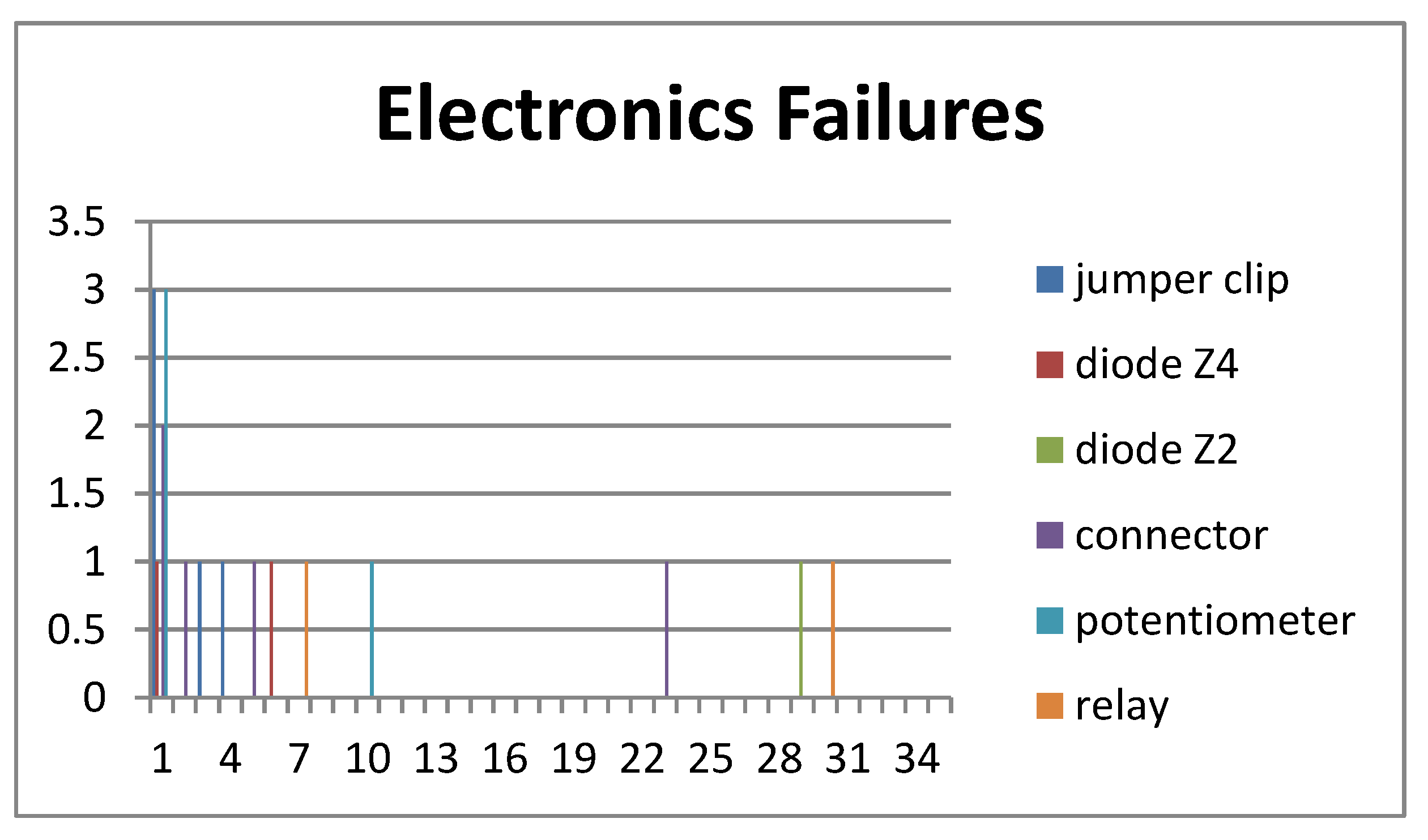
Figure 1. Failure History Pattern.
Inventions 04 00007 g001
Figure 2. Measurement Instrument Failure Events by Failure Mode.
Inventions 04 00007 g002
Figure 3. Measurement Instrument Individual Failure Mode Plots.
Inventions 04 00007 g003
Figure 4. Flow Measurement Instrument Failure Mode Plot of All Electronics Components.
Inventions 04 00007 g004
Figure 5. Life Test Stands in three adjoining rooms.
Inventions 04 00007 g005
Figure 6. Fluid Recirculator with multiple test protocols. (a): Test Setup with −80 °C /+200 °C Fluid Recirculator; (b): Control Screen for −80 °C /+200 °C Fluid Recirculator.
Inventions 04 00007 g006
Figure 7. Dunk Life Test, 300 mm Showcase.
Inventions 04 00007 g007
Figure 8. State of Each Life Test Stand. (a): Executive Summary Status of all Life Test Stands; (b): Detailed Status of Thermal Shock Life Test Stand.
Inventions 04 00007 g008
Figure 9. Thermal Shock Life Stand User Screen.
Inventions 04 00007 g009
Table 1. Flow Measurement Sensor Electronics Failures of 72 Fielded Units.
ElectronicsJumper ClipDiode Z4Diode Z2ConnectorPotentiometerRelayTotal
Number of failures52154219
Number of failures/72 units0.0694444440.0277780.0138890.0694444440.0555555560.0277780.263889
Failures per unit/78,840 h in field8.80828 × 10−73.52 × 10−71.76 × 10−78.80828 × 10−77.04662 × 10−73.52 × 10−73.35 × 10−6

